Graphical model inference with external network data

Abstract

We consider two applications where we study how dependence structure between many variables is linked to external network data. We first study the interplay between social media connectedness and the co-evolution of the andemic across USA counties. We next study study how the dependence between stock market returns across firms relates to similarities in economic and policy indicators from text regulatory filings. Both applications are modelled via Gaussian graphical models where one has external network data. We develop spike-and-slab and graphical rameworks to integrate the network data, both facilitating the interpretation of the graphical model and improving inference. The goal is to detect when the network data relates to the graphical model and, if so, explain how. We found that counties strongly connected on Facebook are more likely to have similar volution (positive partial correlations), accounting for various factors driving the mean. We also found that the association in stock market returns depends in a stronger fashion on economic than on policy indicators. The examples show that data integration can improve interpretation, statistical accuracy, and out-of-sample prediction, in some instances using significantly sparser graphical models.

Keywords: Graphical model, Network data, Spike-and-slab, COVID-19, Stock market, Social media

1 Introduction

We consider two motivating applications where one seeks to learn the dependence structure (partial correlations) across many variables, and is specifically interested in assessing whether said dependence is associated to multiple external network datasets. First, we study the dependence between nfection rates across USA counties, and whether said dependence is linked to network data measuring Facebook connections between counties. This is an important question because individuals who are connected in social networks tend to have similar backgrounds and to be exposed to similar information. Such a shared background may lead to similar attitudes towards health prevention, and hence similar infection risks. For example, allcott2020polarization found that political beliefs were strongly tied to behaviour during the andemic, more specifically that Republicans practised less social distancing. It is hence important to study the association between social media and health outcomes. As described in more detail below, a study by kuchler:2021 found a link between marginal correlations in infection rates between counties and the Facebook index. We propose a probability model that can describe whether and how partial correlations depend on said index, as well as two other networks related to geographical distance and flights passenger traffic. The latter two are meant to help disentangle the effect of two counties being connected on Facebook and their being geographically close or their being major travel between them, i.e. more direct contacts. As a preview of our findings, Figure 1.1 (top) shows estimated (residual) partial correlations between each county pair vs. their geographical closeness and the Facebook index, Figure B.6 contains the corresponding plot for the flights network. Counties that are highly connected on Facebook have a higher proportion of positive partial correlations, whereas for those lowly connected most non-zero partial correlations are negative. Geographically close counties also tend to have positive partial correlations while there does not appear to be a strong relationship between the estimated partial correlations and the flight passenger network. The bottom panels show our spike-and-slab model relating the network data to the probability that a partial correlation is non-zero, and to the mean and variance of the non-zero partial correlations.

As a second application, we study the dependence of stock market excess returns across companies, incorporating external data on similarities between companies in their exposure to economic and policy risks (as defined by bakerPolicyNewsStock2019). Said risks were extracted from text data in mandatory regulatory filings where companies must disclose potential risks, and the idea is that if two companies disclosed similar economy- or policy-related risks then it may be more likely that they have similar stock market returns. The applied relevance of the problem arises from the longstanding insight in finance that the dependence among assets informs optimal portfolios (markowitzPortfolioSelection1952). In particular, the precision matrix determines the weights across assets that minimise a portfolio’s standard deviation. Bringing optimal portfolio theory to data requires estimating high-dimensional covariance/precision matrices, which is an important barrier to its practical application (eltonEstimatingDependenceStructure1973). A variety of approaches have been used to tackle the problem including, recently, gotoImprovingMeanVariance2015, see also senneretCovariancePrecisionMatrix2016 for an empirical review. A critical observation is that we seek not only to estimate the partial correlations featuring in the precision matrix, but also to portray how they may depend on the text-based economic and policy risks, to shed light onto the joint behavior of stock market returns.

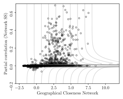
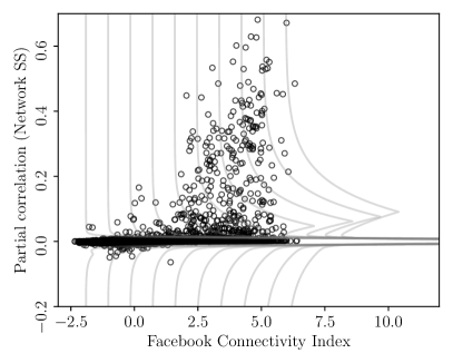
Figure 1.1: Residual partial correlations in nfections (adjusted for covariates) across counties vs Geographical Closeness Network defined as $1/\log(Geodistance)$ (left) and log-Facebook Connectivity Index (right). Top panel: partial correlations estimated with graphical LASSO, with penalization parameter set via Bottom panel: fitted spike-and-slab distributions and fitted partial correlations estimated with network graphical spike-and-slab LASSO.

We use Gaussian graphical models (GGMs) and extensions discussed later as a convenient framework that describes the dependence among random variables in an interpretable manner, providing a suitable basis for our applications. There are however certain challenges that led us to develop a methodological framework that is another main contribution of this paper, and can be applied to numerous applications other than those considered here.

A first applied challenge is that the ease with which one can interpret the output of a graphical model deteriorates as the number of variables $p$ gets large, i.e. there are simply too many edges to read them one by one. Our proposed model provides a way to regress the probability of an edge being present, as well as the mean and variance of the associated (non-zero) partial correlation, on external network data. Said regression helps understand when one can expect an edge to be present, and to have a certain sign and magnitude, as illustrated in Figure 1.1. A second challenge is that in our applications the sample size $n$ is moderate relative to the $p(p+1)/2$ covariance parameters. By integrating external network data one hopes to improve the accuracy of the inference, provided said data carries useful information regarding the graphical model. Our framework provides natural novel strategies to assess whether the network data is indeed useful.

To our knowledge, there are no model-based methods to incorporate multiple network-valued external data in undirected graphical models. There has been, however, active research on incorporating external data in regression. For example, stingo:2010 proposed a multivariate regression of gene expression on micro-RNA, where the prior probabilities that micro-RNAs have a non-zero coefficient depend on an external biological and structural similarity score. Similarly, stingo:2011 incorporated pathway information into regression models for gene expression, quintana_ma:2013 proposed a Bayesian variable selection framework where prior inclusion probabilities depend on meta-covariates, cassese:2014 a multivariate regression of gene expression versus copy number variations that incorporates their physical distance in the genome, peterson2016joint a regression framework using a network for covariate penalisation, and chiang:2017 a brain activity vector auto-regression that incorporates external brain information. chen_tinghuei:2021 predicted disease outcomes given single nucleotide polymorphisms, where the egularisation parameter depends on functional annotation categories.

There has also been work incorporating network data in graphical models, primarily in neuroscience. ng2012novel; pineda2014guiding; higgins2018integrative considered penalised likelihood GGMs to understand co-activation across brain regions, where one has strong grounds to believe that external network data extracted from known brain structure provides useful information. In a similar vein, bu2021integrating use distances between brain regions to drive the regularisation of a GGM that is fit via multiple univariate regressions, and provide theoretical conditions for asymptotic learning of the GGM’s structure. The main applied difference with our setting is that we wish to assess whether the network data are informative and, if so, depict how. Another difference is that we consider multiple network datasets (e.g. Facebook, distance, flights), rather than only one. In simulations we illustrate how assessing whether the network data are useful or not can lead to significant practical improvements. As discussed, the main methodological difference is that we develop a probabilistic spike-and-slab model to regress the GGM on the network data that helps interpret the presence of edges and the sign and magnitude of partial correlations. This is important in our applications, e.g. the bottom panels in Figure 1.1 depict that large Facebook connectivity is associated with positive partial correlations.

We develop two frameworks to integrate network data into GGM selection and parameter estimation. The first framework is a hierarchical extension of the graphical (friedman:2008; yuan2007model, see also wang_hao:2012 for a discussion of Bayesian counterparts). The framework largely follows that in ng2012novel, except that we learn critical hyper-parameters from data and assess whether each network data is actually useful or not. We also develop tailored optimisation algorithms that build on the lgorithm of lauritzen:2020 so that the computational cost is similar to a standard roblem, and we apply Bayesopt algorithms to speed up the search over hyper-parameter values. Our second framework is the main contribution and uses a spike-and-slab prior, with the novel feature that the slab’s probability, location and variance are regressed on the network data. To ensure its practical applicability we developed a software implementation in the probabilistic programming languages Stan (carpenter:2017) and NumPyro (bingham:2019; phan:2019). The latter capitalises on efficient automatic differentiation and GPUs to help boost the computational speed. Similarly, the first framework is implemented in R.

The paper proceeds as follows. Section 2 discusses our motivating applications in more detail. Section 3 reviews the introduces our network-adjusted extension and its Bayesian analogue. Section 4 discusses our computational strategy for learning the graphical model and hyper-parameters that depict its association with the external network data. Section 5 uses simulations to shed light on a natural practical question: what if the network data are useless, i.e. uninformative regarding the graphical model we seek to learn? We illustrate that one should assess whether the network data have useful information about the GGM and, if not, discard them to avoid deteriorating inference. Section 6 shows our main results for the nd stock market applications, and Section LABEL:sec:discussion concludes. Code to implement all of our experiments and data pre-processing is available at https://github.com/llaurabat91/graphical-models-external-networks.

2 Motivating applications

2.1 Dependence in nfections versus Facebook, geographical and flight networks

Studying the evolution of pandemics such as s of great importance for health, economic and societal reasons. There are many studies to forecast infections or to understand how they are related to various factors (e.g. health measures, temperature). We consider a further important aspect that received less attention: understanding how the disease co-evolves across (possibly distant) geographical units, and what factors are associated to such co-evolution. For example, if several counties were expected to simultaneously exhibit higher-than-expected infection rates, health authorities might need to plan resources accordingly. Further, identifying factors that are related to the co-evolution (e.g. the Facebook index) may suggest strategies to limit such coordinated growth (e.g. targeted information campaigns).

To study o-evolution across USA counties, we downloaded weekly infection rates from COVID:2020 for the period 22 January 2020 to 30 November 2021 (97 weeks total) for all USA counties ($>3,000$ in total). We then iteratively clustered neighbouring counties with small population until all aggregated counties had at least 500,000 inhabitants, obtaining 332 aggregated counties in total. Full details of our clustering procedure are presented in Section B.3. For simplicity onwards we refer to aggregated counties simply as counties. The reason for clustering counties was two-fold. First, the weekly infection rates for smaller counties are subject to high variance, and hence less reliable than when grouping counties. Second, working with $>3,000$ counties results in a GGM with $>4,500,000$ parameters, which imposes serious computational bottlenecks.

We also obtained data on covariates that are thought to be associated with the disease’s evolution, such as temperature, population density, vaccination rates and an index measuring the stringency of pandemic measures (Temperature:2020; Population:2020; Vaccination:2020; Policy:2020). We defined the outcome of interest as the county log-infection rates, i.e. log infections relative to the county’s population. Our interest is in studying the disease co-evolution after accounting for factors driving the mean structure. To this end, we fitted a linear regression model that included temperature, vaccination rates, the stringency of pandemic measures, a weekly fixed effect term estimating the mean infections across all counties in that particular week, and a first-order auto-regressive term measuring the infection rate in the previous week. See Section B and the supplementary code for the data collection, pre-processing, and residual checks assessing the linearity and normality assumptions, and that higher-order auto-regressive terms are not needed.

Although the mean model explained most of the variance in infection rates (adjusted $R^{2}$ coefficient 0.942), certain county pairs were systematically both above or below the model predictions. Specifically, we estimated partial correlations in the regression residuals for each county pair via graphical LASSO, and obtained numerous non-zero estimates (Figure 1.1, top). Said partial correlations indicate that certain county pairs tend to behave better or worse than expected (given the week’s overall pandemic status and other covariates) in a coordinated fashion. Our primary goal is to assess whether this coordinated behavior occurs more frequently across counties that are strongly connected via social media, given by the Facebook index. Said index defines a network of counties, measuring the strength of the connection between every pair of counties. We also consider two further networks, one based on geographical closeness (see Section 6.1) and a second measuring flow of passengers between two counties by plane (see Section B).

We see partial correlations as an appealing measure of disease co-evolution. For example, suppose that infections in County A drive those of County B, which in turn drive those of County C, then all three counties would have non-zero marginal correlation. In contrast, the partial correlation between counties A and C would be zero, suggesting there is no direct link between them. An important observation stemming from Figure 1.1 is that counties that are highly connected on Facebook have a higher proportion of non-zero, and positive, partial correlations. A similar observation applies to geographical distances. Hence one wishes not only to regularise to a lesser extent county pairs with a strong Facebook connection but also to describe how the average non-zero partial correlation depends on Facebook (or geographical, or flight) connectivity. This desideratum led us to develop a network-regularised spike-and-slab framework, where the slab’s mean, variance and probability are regressed on the network, see Section 3.

2.2 Dependence in stock market returns versus text data

Our goal is to study whether and how covariation in stock market excess returns (i.e. returns above/below those that were expected, see below) across firms is associated with firms’ sharing similar risks. To measure to what extent they do so, we downloaded text of the Risk Factors (RF) section of publicly traded firms’ annual 10-K filings to the USA Securities and Exchange Commission. For each firm, we combine all filings made between 2015 and 2019, inclusive. Said filings describe exhaustively future earnings risks faced by the firms, and there is an incentive for full disclosure because investors can take legal action when firms withhold information that if disclosed would have prevented financial losses. Firms that face similar risks may have more dependent stock returns, e.g. two firms mentioning risks to oil price rises may co-move when oil prices change. Indeed, hanleyDynamicInterpretationEmerging2019 regressed the covariance of excess returns between pairs of financial firms on a measure of RF text overlap and showed a positive relationship in the lead-up to the global financial crisis in 2008. More recently, davisFirmLevelRiskExposures2020 shows that firms with similar RF texts reacted similarly to the arrival of Our analysis goes beyond these studies by modelling partial rather than marginal correlations. We also allow distance in RF-text space to influence both the probability of a connection between firms and the mean (and variance) of the partial correlations on the network.

We consider $p=366$ firms traded on US markets that satisfy the following conditions: i) membership in S&P500 at the end of 2019; ii) closing stock price adjusted for stock splits and dividends available in the COMPUSTAT database for every trading day between 2 January 2019 to 31 December 2019 (252 trading days in total); iii) at least one 10-K filing available in 2014-2019. For each trading day in 2019 we construct daily excess returns using the Fama-French three-factor model. Specifically, we individually regress each firm’s daily log-returns on the variables contained in the daily, three Fama/French factors file downloaded from Kenneth French’s Data Library website. The residual is the excess return.

To measure textual similarity between companies, we first construct a bag-of-words representation of each firm’s 10-K filings during 2014-2019. We follow bakerPolicyNewsStock2019, and compute firms’ exposure to 16 separate economic risks and 20 separate policy risks. For each risk $r$, bakerPolicyNewsStock2019 define a term set $T_{r}$ containing terms that reflect the exposure. For example, the policy risk ‘food and drug policy’ is captured by the term set $\{$prescription drug act, drug policy, food and drug administration, fda$\}$. bakerPolicyNewsStock2019 show that intertemporal variation in economic and policy risk terms in newspaper articles closely tracks aggregate market volatility. This motivates the idea of using variation in these terms across individual firms to better measure their co-movement across trading days.

Let $x_{i,v}$ be the count of term $v$ in firm $i$’s 10-K filings during 2014-2019 and let $C_{i}\equiv\sum_{v}x_{i,v}$ be the total number of terms. We measure each firm’s exposure to risk $r$ as $\log\left(1+\sum_{v\in T_{r}}x_{i,v}/C_{i}\right)$, i.e. logarithm of 1 plus the proportion of words referring to risk $r$ out of the total $C_{i}$ words. We use the logarithm to account for the fact that a risk term not being mentioned at all versus being mentioned once is likely to be more informative than being mentioned many times compared with slightly more times. For each pair of firms, we then measure its similarity in exposure to economic risks by computing the correlation between the vector of economy-related risks. This defines a network between companies such that the network connection between companies $(j,k)$ is given by said correlation. We proceeded analogously to define a policy risk network by computing correlations between policy-related terms.

In summary, our data processing produced two networks between firms that measure their similarity in risk exposures based on a particular representation of RF texts. We remark that one could use alternative text analysis tools, however our goal is to establish that text-based relational data can be useful to estimate dependence in stock returns. The optimal representation of text for this task is left as an open question. Still, as we show below, separately controlling for economic and policy risks yields important insights regarding whether government policy generates return co-movement above and beyond that generated by firm fundamentals.

See Section C and the supplementary code for the data collection, pre-processing, linear model fit, and residual checks assessing our model assumptions.

3 Model

We describe two model-fitting strategies to regress an undirected GGM on $p$ variables onto multiple external network datasets. Section 3.1 discusses network which we mainly use as a computationally-convenient framework to assess whether one should add/remove each network dataset. We also discuss a Bayesian interpretation useful to check that the assumed model fits the observed data. Section 3.2 is our main contribution, a spike-and-slab model to regress partial correlations on network data. Section 3.3 discusses how to extend our framework beyond Gaussian data, as needed for the stock market application.

We set notation. Let $y_{i}\in\mathbb{R}^{p}$ be the outcome vector for individuals $i=1,\ldots,n$ (e.g. log-infection rates in $p$ counties at week $i$, or stock excess returns for $p$ companies at day $i$) and $x_{i}\in\mathbb{R}^{d}$ covariates (week indicator, temperature, percentage of fully vaccinated individuals in week $i$, etc.). We assume that $y_{i}\sim\mathcal{N}_{p}\left(Bx_{i},\Theta^{-1}\right)$ independently across $i=1,\ldots,n$, where $B$ is a $p\times d$ regression coefficients matrix and $\Theta$ a $p\times p$ positive-definite precision (or inverse covariance) matrix. To ensure that the independence assumption across $i$ is tenable, we include lagged versions of $y_{i}$ into the covariates $x_{i}$, as described in Section 2 and B. For simplicity, in our applications we start by subtracting the estimated mean $\hat{B}x_{i}$ from $y_{i}$, where $\hat{B}$ is the least-squares estimator, and subsequently assume the outcomes to have zero mean, i.e. $y_{i}\sim\mathcal{N}_{p}(0,\Theta^{-1})$.

A convenient property of modelling $y_{i}\sim\mathcal{N}_{p}\left(0,\Theta^{-1}\right)$ is that conditional independence statements can be drawn from the graph defined by the non-zero elements of $\Theta$. Specifically, $(y_{ij},y_{ik})$ are independent given the remaining elements in $y_{i}$ if and only if $\Theta_{jk}=0$. As argued earlier, in our applications we use partial correlations as a measure of association. We denote partial correlations by

$$\rho_{jk}:=\textrm{corr}(y_{ij},y_{ik}\mid y_{i\{1,\ldots,p\}\setminus\{j,k\}})=-\frac{\Theta_{jk}}{\sqrt{\Theta_{jj}\Theta_{kk}}}.$$ (3.1)

Importantly, in our framework, one also observes external data in the form of $Q\geq 1$ networks between variables. These are $p\times p$ symmetric matrices $A^{(1)},\ldots,A^{(Q)}$, where $a^{(q)}_{jk}$ measures strength of the connection between variables $(j,k)$. In the pplication $a^{(1)}_{jk}$ is the geographical closeness between counties $(j,k)$, $a^{(2)}_{jk}$ their Facebook connection index, and $a^{(3)}_{jk}$ their flight connectivity. In the stock application, $a^{(1)}_{jk}$ is the similarity between firms $(j,k)$ in their exposure to economic risks, and analogously $a^{(2)}_{jk}$ for policy risks.

3.1 Network graphical LASSO

Network graphical LASSO is a penalised likelihood framework to estimate $\Theta\in\mathcal{S}^{p}_{+}$ by maximising a Gaussian log-likelihood plus a graphical penalty (friedman:2008; yuan2007model), where the magnitude of said penalty is regressed onto the network datasets. Specifically, we consider

$$\hat{\Theta}=\operatorname*{arg\,max}_{\Theta\in\mathcal{S}^{p}_{+}}\;\;\;\log\det(\Theta)-\textrm{tr}(S\Theta)-\sum_{j\neq k}\lambda_{jk}|\Theta_{jk}|,$$ (3.2)

where $\mathcal{S}^{p}_{+}$ is the set of non-negative definite matrices, $\textrm{tr}(\cdot)$ the matrix trace, $S$ the empirical covariance matrix of $(y_{1},\ldots,y_{n})$,

$$\lambda_{jk}=\lambda_{jk}(A^{(1)},\ldots,A^{(Q)})=\exp\left\{\beta_{0}+\sum_{q=1}^{Q}\beta_{q}a_{jk}^{(q)}\right\}$$ (3.3)

are regularisation parameters, and $\beta=(\beta_{0},\ldots,\beta_{Q})\in\mathbb{R}^{Q+1}$ are regularisation hyperparameters that play a critical role in determining the level of sparsity in $\hat{\Theta}$. That is, each $\Theta_{jk}$ gets a potentially different penalty parameter $\lambda_{jk}$, which is a function of the network data $A^{(1)},\ldots,A^{(Q)}$. To simplify notation, we omit the dependence on $A^{(1)},\ldots,A^{(Q)}$ and simply use $\lambda_{jk}$, and let $A=(A^{(1)},\ldots,A^{(Q)})$. For convenience we parameterise the penalties in terms of a scaled version of $A^{(q)}$ that is centered to have zero sample mean and unit sample variance, and which we denote by $\bar{A}^{(q)}$. s the particular case where $\lambda_{jk}$ are constant across $(j,k$).

ng2012novel proposed the penalty in (3.2)-(3.3), the main difference being that we consider multiple networks ($Q>1$) and that we learn hyper-parameters $\beta$ from data, including the exclusion of some networks. Two popular strategies to set hyper-parameters are using cross-validation (friedman:2008) and information criteria such as the Bayesian information criterion ( (schwarz:1978). The former is more suitable for predictive tasks than when seeking models that help explain the data-generating truth, e.g. cross-validation does not lead to consistent model selection even in simpler linear regression where the nd related information criteria are consistent, see foygel2010extended; zhang_yiyun:2010; wang_tao:2011; fan_yingying:2013. We hence use the o learn $\beta$. Specifically, viewing $\hat{\Theta}(\beta)$ as a function of $\beta$, we choose $\beta$ minimising

$$\hat{\beta}_{\lx@acro@@@def{\smaller BIC}{\smaller BIC}{}{{\smaller BIC}}{{}}}:=\operatorname*{arg\,min}_{\beta\in\mathbb{R}^{Q+1}}\lx@acro@@@def{\smaller BIC}{\smaller BIC}{(}{{\smaller BIC}}{{(}}\beta) \;=\;-2\ell_{n}(\hat{\Theta}(\beta))+\big{|}\mathbf{E}(\hat{\Theta}(\beta))\big{|}\cdot\log n,$$ (3.4)

where $\ell_{n}(\hat{\Theta})$ is the Gaussian log-likelihood function and $|\mathbf{E}(\hat{\Theta}(\beta))|$ counts the number of edges in the graph associated with $\hat{\Theta}(\beta)$. Importantly, note that when $\beta_{q}=0$ then the $q^{th}$ network dataset is effectively excluded. The idea is that if a network dataset does not provide useful information about $\Theta$, then one may set $\beta_{q}=0$ to avoid adding unnecessary noise to $\hat{\Theta}$, see Section 5 for an illustration. An alternative to the s the Extended (chen:2008). As a sensitivity check, we provide results using the o select $\beta$ in Sections A.5, B.8 and C.6. In our examples the as overly conservative in selecting edges, which resulted in high mean-squared-error. Finally, we note that there are alternative approaches to choosing $\beta$, see kuismin, but they require more extensive computations that become prohibitive in our setting. We also note that alternatives to (3.2) include the adaptive graphical LASSO, SCAD and MCP (fan:2009; wang_lingxiao:2016), which were proposed to reduce bias in the estimation of large entries in $\Theta$. We focus on (3.2) however due to its practical appeal of defining a concave problem for which one may establish efficient optimisation methods.

One could of course consider alternative parameterisations to (3.3), e.g. let $\lambda_{jk}$ depend non-parametrically on the network data. However, (3.3) requires fewer hyper-parameters than a non-parametric treatment and is easy to interpret: the log-regularisation depends linearly on the networks. Further, a model-checking exercise suggested that (3.3) is a reasonable parameterisation for our two motivating applications. Said model-checking is best understood by adopting a Bayesian interpretation. The penalised estimator associated to (3.3) is equivalent to the posterior mode under independent Laplace priors (wang_hao:2012) with scale parameter $1/\lambda_{jk}$, that is

$$\pi(\Theta\mid A,\beta)\;\propto\;\prod_{j>k}\frac{\lambda_{jk}}{2}\exp\left\{-\lambda_{jk}|\theta_{jk}|\right\}\mbox{I}(\Theta\succ 0),$$ (3.5)

where $\mbox{I}(\Theta\succ 0)$ is an indicator for $\Theta$ being positive-definite, $\lambda_{jk}$ is as in (3.3) and $\beta$ are now prior parameters. The Bayesian interpretation is that the $\lambda_{jk}$’s arise from a Laplace random effects distribution with parameter $\beta$. The a priori expected value of $\theta_{jk}$ is 0, which induces sparsity, and the prior variance is

$$\textrm{Var}\left[\theta_{jk}~{}|~{}\beta,A\right]=\mathbb{E}\left[\theta_{jk}^{2}~{}|~{}\beta,A\right]=\frac{2}{\lambda_{jk}^{2}}.$$ (3.6)

Therefore (3.3) assumes that the log-variance of the partial covariances $\theta_{jk}$ depends linearly on the network data

$$\log\mathbb{E}\left[\theta_{jk}^{2}~{}|~{}\beta,A\right]=\log(2)-2\left(\beta_{0}+\beta_{1}\bar{a}^{(1)}_{jk}+\ldots+\beta_{Q}\bar{a}^{(Q)}_{jk}\right).$$ (3.7)

Provided one has an initial estimate of the left-hand side of (3.7), which in our examples we derived from standard stimates of $\theta_{jk}$, one may check whether its relation to the network data is roughly linear. Such a check motivated taking the logarithm of the raw distances, Facebook connectivities and flight passenger flow to define our networks for the ata, while the stock market risk indicator networks required no transformations. See Supplementary Sections B.6 and C.4 for further details.

3.2 Network graphical spike-and-slab LASSO

The network graphical LASSO in (3.2) provides sparse point estimates of partial correlations and, via its Bayesian interpretation, describes how their variance depends on the network data. In our applications, however, we also seek to describe how the proportion of non-zero partial correlations and their mean depend on the network. For example, in the ata both the probability that two counties are conditionally dependent and the mean partial correlation grow as their Facebook connection grows (Figure 1.1), and similarly for the stock market data (Figure C.5). To address this issue, we developed a spike-and-slab framework that builds on the regression setting of rockova:2014 and the graphical spike-and-slab of gan:2018. The main novelty is that both the slab prior probability and its parameters depend on network data. In particular, the slab need not be centered at zero, a feature that is novel—to our knowledge—and has some independent interest.

We parameterise $\Theta$ in terms of partial correlations $\rho_{jk}$ in (3.1), which facilitates interpretation and ensures that the posterior mode is invariant to scale transformations. By scale invariance we refer to the property that the estimated $\rho_{jk}$ remain the same regardless of whether one applies a scale transformation to the input data or not, see carter2021partial for a detailed discussion. We set a prior density $\pi(\mbox{diag}(\Theta),\rho)=\pi(\mbox{diag}(\Theta))\pi(\rho)$, where $\sqrt{\Theta_{ii}}\sim\mathcal{IG}(a,b)$ with $a=0.01$ and $b=0.01$ reflecting an uninformative prior on the diagonal elements of $\Theta$, and

$$\pi(\rho\mid\eta) =C_{\eta}\mbox{I}(\rho\succ 0)\prod_{j>k}(1-w_{jk})\mbox{DE}(\rho_{jk};0,s_{0})+w_{jk}\mbox{DE}\left(\rho_{jk};\eta_{0}^{T}a_{jk},s_{jk}\right)$$ (3.8)

$$w_{jk} =\left(1+e^{-\eta_{2}^{T}a_{jk}}\right)^{-1},\quad s_{jk}=s_{0}(1+\exp\left\{\eta_{1}^{T}a_{jk}\right\}),$$

where $C_{\eta}$ is the normalisation constant and $\mbox{I}(\rho\succ 0)$ a positive-definiteness indicator. The spike is a double-exponential with zero mean and small scale $s_{0}$ meant to capture partial correlations that are practically zero, whereas the slab has larger variance $s_{jk}$ and may not be centered at zero. The slab prior probability $w_{jk}$ follows a logistic regression on the network data $a_{jk}=(1,a_{jk}^{(1)},\ldots,a_{jk}^{(Q)})$, its mean $\eta_{0}^{T}a_{jk}$ depends linearly on $a_{jk}$ and its variance $s_{jk}$ is larger than $s_{0}$ by a factor that also depends on $a_{jk}$. Specifically, positive entries in $\eta_{0}$ and $\eta_{1}$ indicate that the mean and variance (respectively) of the non-zero partial correlations increase for larger network connections $a_{jk}$, and similarly positive $\eta_{2}$ indicates a higher probability of a non-zero partial correlation for large $a_{jk}$.

We remark that because of the constraint $\mbox{I}(\rho\succ 0)$ the marginal prior $\pi(\rho_{jk})$ could be fairly different from the unconstrained density inside the product in (3.8), then $w_{jk}$ could not be interpreted as the prior probability of an edge, and similarly for $\eta_{0}^{T}a_{jk}$ and $s_{jk}$. To address this issue we elicit prior parameters such that the indicator $\mbox{I}(\rho\succ 0)$ is satisfied with high prior probability, see below.

Above $\eta=(\eta_{0},\eta_{1},\eta_{2})\in\mathbb{R}^{3(Q+1)}$ are hyper-parameters driving the regression model of the partial correlations $\rho_{jk}$ onto the network data $a_{jk}$, and are a main quantity of interest in our applications. A standard strategy to set prior hyper-parameters such as $\eta$ in (3.8) is an empirical Bayes framework where one maximises the marginal likelihood. Such a framework allows us to do inference on the $\eta$’s themselves through the marginal posterior $\pi(\eta\mid y)$ and inference for $\Theta$ through the empirical Bayes posterior

$$\pi(\Theta|y,\hat{\eta})=f(y|\Theta)\pi(\Theta|\hat{\eta}),$$

where $\hat{\eta}$ maximises the marginal posterior of $\eta$ given the data

$$\hat{\eta}: =\operatorname*{arg\,max}_{\eta}\pi(\eta\mid y)=\operatorname*{arg\,max}_{\eta}\int\pi(\Theta,\eta|y)d\Theta=\operatorname*{arg\,max}_{\eta}\int f(y|\Theta)\pi(\Theta|\eta)\pi(\eta)d\Theta.$$

One could consider using the joint posterior $\pi(\Theta,\eta|y)$ for inference on $\Theta$ and $\eta$, but we found empirical Bayes to perform better in our experiments. See giannoneEconomicPredictionsBig2021 for a related discussion on the desirability to learn the appropriate degree of sparsity from data in social science applications, and a related spike-and-slab proposal in a regression setting.

We next discuss our default elicitation for the prior $\pi(\rho\mid\eta)$. The guiding principle was to set a minimally-informative prior, so that data may suitably update prior beliefs, while encouraging sparse solutions and preserving the interpretability of (3.8). Briefly, we set $\pi(\eta)$ to be proportional to $C_{\eta}^{-1}$ times independent Gaussian prior densities on $(\eta_{0},\eta_{1},\eta_{2})$. Adding the term $C_{\eta}^{-1}$ is a trick to simplify computation, since then $C_{\eta}$ drops from the posterior density $\pi(\Theta,\eta\mid y)$. wang_hao:2015 argued that such cancellation of prior normalisation constants does not adversely affect spike-and-slab priors in graphical model settings (as long as the constant affects hyper-parameters $\eta$ but not parameters $\Theta$, as in our case). The prior on $\eta_{2}$ was set such that the prior mean number of edges is proportional to $p$, which induces sparsity, and the prior sample size can be thought of as 1, in analogy to the standard default Beta(0.5,0.5) prior in a Binomial experiment. The prior on $\eta_{1}$ was set such that the prior mode of the slab’s scale is $10s_{0}$ and greater than $3s_{0}$ with probability 0.99, i.e. the slab captures partial correlations of a larger magnitude than the slab. Finally, the prior on $\eta_{0}$ was set such that the slab has zero prior mean and such that sampling entries of $\rho$ independently from the double-exponential priors in (3.8) returns a positive-definite matrix with 0.95 prior probability. This ensures that $\pi(\rho\mid\eta)$ is similar to its unconstrained version where one drops the positive-definiteness indicator, as otherwise $w_{jk}$ cannot be interpreted as the marginal slab probability.

Figure A.1 plots the implied prior marginal distribution on the $\rho_{jk}$’s for both the nd stock market applications showing that the prior concentrates at 0 but also features thick tails to capture true non-zero $\rho_{jk}$’s. The corresponding posteriors (Figure A.1, bottom panels) set significant mass away from zero, suggesting that the prior shrinkage towards 0 was not excessive. Section A.3 provides further details and lists the hyper-parameter values used in our examples. Our code contains an implementation of our prior elicitation method.

3.3 Beyond Gaussian data

In certain applications such as our stock market example, data exhibit non-Gaussian behavior such as thick tails and asymmetries, even after taking logarithmic or similar transforms (see the normality checks in Section C.3). To address this issue in this application we used a non-paranormal model, which can accommodate said departures from normality. The distribution of $y_{i}=(y_{i1},\ldots,y_{ip})$ is non-paranormal if there exist strictly increasing functions $f_{j}:\mathbb{R}\to\mathbb{R}$ for $j=1,\ldots,p$ such that the vector $f(y_{i}):=(f_{1}(y_{i1}),\ldots,f_{p}(y_{ip}))$ is Gaussian. Such a non-paranormal model may be estimated by first obtaining an estimate $\hat{f}$ from the data, for which we used the R package huge (zhao2012huge), and subsequently applying our methodology to the transformed data $\hat{f}(y_{i})$.

An interesting property of the non-paranormal family is that the graphical model can be interpreted as in the Gaussian case. The partial correlation between the transformed $f_{j}(y_{ij})$ and $f_{k}(y_{ik})$ is zero if and only if $(y_{ij},y_{ik})$ are conditionally independent. Partial correlations retain an interesting interpretation in the trans-elliptical family: zero partial correlation $\rho_{jk}=0$ indicates that $y_{ij}$ is linearly independent with any transformation of $y_{ik}$ (rossell2021dependence).

4 Computation and inference

4.1 Network

We first describe how to optimise (3.2) for a fixed $\beta$, and subsequently how to estimate $\hat{\beta}$. The main idea is that, since $\lambda_{jk}=\lambda_{jk}\left(A,\beta\right)$ are fixed for a fixed $\beta$, the network bjective in (3.2) is a special case of the lass of models in lauritzen:2020. Motivated by the desire to penalise positive and negative partial correlations differently, lgorithms consider Gaussian graphical models with likelihood penalties of the form

$$\sum_{j=1}^{p}\sum_{k\neq j}\max\left\{L_{jk}\rho_{jk},U_{jk}\rho_{jk}\right\},$$ (4.1)

where $-\infty\leq L_{jk}\leq 0\leq U_{jk}\leq\infty$ are fixed. Noting that $\lambda|x|=\max\left\{-\lambda x,\lambda x\right\}$ for positive $\lambda$, we see that the penalty in (3.2) is in the form of (4.1) with $L_{jk}=-\lambda_{jk}$ and $U_{jk}=\lambda_{jk}$. (3.2) is a convex problem that can be efficiently solved using a block-coordinate ascent algorithm similar to that proposed for n (banerjee2008model). An R package is provided for t https://github.com/pzwiernik/golazo.

Obtaining $\hat{\beta}_{\lx@acro@@@def{\smaller BIC}{\smaller BIC}{}{{\smaller BIC}}{{}}}$ requires maximising $\lx@acro@@@def{\smaller BIC}{\smaller BIC}{(}{{\smaller BIC}}{{(}}\beta)$ in (3.4). As usual when using information criteria to set regularisation parameters, this is a non-concave function of $\beta$ that exhibits discontinuities. We propose two optimisation approaches. In cases where only one or two external networks are available and $p$ is moderate ($p\leq 200$, say) we propose a grid-search akin to that used to set the regularisation parameter in standard Section A.1 contains several analytic upper bounds to facilitate such a search. However, the dimension of the hyper-parameter $\beta$ grows with the number $K$ of external networks, hence grid searches are very costly when $K\geq 3$ and $p$ is large. In these settings, we propose using Bayesian optimisation. Briefly, Bayesian optimisation first evaluates the objective function $\lx@acro@@@def{\smaller BIC}{\smaller BIC}{(}{{\smaller BIC}}{{(}}\beta)$ at a few values of the hyper-parameter $\beta$ and uses a Gaussian process to estimate $\lx@acro@@@def{\smaller BIC}{\smaller BIC}{(}{{\smaller BIC}}{{(}}\beta)$ for all $\beta$. Next, an acquisition function to propose new $\beta$ values at which to evaluate $\lx@acro@@@def{\smaller BIC}{\smaller BIC}{(}{{\smaller BIC}}{{(}}\beta)$, which are then used to update the Gaussian process estimate. In particular we use the R  package rBayesianoptimisation (yan2016rbayesianoptimization), with the ‘ucb’ acquisition function and maximum function evaluations as 15 + 5$Q$, where $Q$ is the number of considered networks. In our examples Bayes optimisation returned virtually identical results to a grid search, but incurred a significantly lower computational cost when $\lx@acro@@@def{\smaller BIC}{\smaller BIC}{(}{{\smaller BIC}}{{(}}\beta)$ is hard to evaluate by requiring many fewer evaluations compared with the grid search alternative.

4.2 Spike-and-slab

The full parameter of interest is $(\mbox{diag}(\Theta),\rho,\eta)$, where $\eta=(\eta_{0},\eta_{1},\eta_{2})$ are the hyper-parameters in (3.8). To approximate their posterior distribution $\pi(\mbox{diag}(\Theta),\rho,\eta\mid y)$ given the data $y$ we used Hamiltonian Monte Carlo (see neal:2011 for a review). Specifically, we developed an R implementation using the Stan software (carpenter:2017), as well as a Python implementation using the NumPyro package (phan:2019). Sections A.2 and A.4 describe further implementation details and our code provides both implementations. The purpose of the R version is to make our methods available to the ample R community, whereas NumPyro provides significant computational savings by using improvements in automatic differentiation and enabling the use of GPUs. The savings were substantial, Section D demonstrates that greater than an order of magnitude speed up was possible even in simple experimental settings.

The output of both implementations are $N$ posterior samples $(\mbox{diag}(\Theta^{(i)}),\rho^{(i)},\eta^{(i)})$ for $i=1,\ldots,N$ that can be used to approximate the posterior distribution or suitable summaries such as the marginal posterior mean and standard deviation of any parameter. Of particular interest to us is to estimate the posterior probability for the presence of an edge between any two nodes $(j,k)$, i.e. that the partial correlation $\rho_{jk}$ was generated by the slab in (3.8). We next discuss how to estimate said posterior probability using the posterior samples.

To ease notation re-write the prior as

$$\pi(\rho_{jk}\mid\eta) =(1-w_{jk}(\eta))\pi_{0}(\rho_{jk}\mid\eta)+w_{jk}(\eta)\pi_{1}(\rho_{jk}\mid\eta)$$ (4.2)

where $\pi_{0}(\rho_{jk}\mid\eta)$ is the spike prior density, $\pi_{1}(\rho_{jk}\mid\eta)$ the slab prior density, and $w_{jk}(\eta)$ the slab prior probability. The idea is that any $\rho_{jk}$ generated by the spike takes a near-zero value, i.e. the partial correlation is either truly zero or small enough to be practically irrelevant. Let $z_{jk}=1$ indicate that $\rho_{jk}$ was generated from the slab and $z_{jk}=0$ that it was generated from the spike, i.e. $P(z_{jk}=1\mid\eta)=w_{jk}$. A measure of evidence in favor of the presence of the edge is the posterior probability

$$P(z_{jk}=1\mid y)=\int P(z_{jk}=1\mid\rho_{jk},\eta)\pi(\rho_{jk},\eta\mid y)d\rho_{jk}d\eta,$$ (4.3)

where from Bayes rule

$$P(z_{jk}=1\mid\rho_{jk},\eta)=\frac{w_{jk}(\eta)\pi_{1}(\rho_{jk}\mid\eta)}{(1-w_{jk}(\eta))\pi_{0}(\rho_{jk}\mid\eta)+w_{jk}(\eta)\pi_{1}(\rho_{jk}\mid\eta)}.$$ (4.4)

Given $B$ posterior samples from $\pi(\rho,\eta\mid y)$, (4.3) may be easily estimated by

$$\hat{P}(z_{jk}=1\mid y)=\frac{1}{N}\sum_{I=1}^{N}P(z_{jk}=1\mid\rho_{jk}^{(I)},\eta^{(I)})$$ (4.5)

The description above applies in a full Bayesian treatment where $\eta$ has a posterior distribution, in our empirical Bayes framework we simply replaced $\eta$ by $\hat{\eta}$ in (4.2)-(4.5).

Our decision rule is to include edge $(j,k)$ whenever $\hat{P}(z_{jk}=1\mid y)\geq t$ for some threshold $t\in[0,1]$. We used $t=0.95$. In problems where the goal is to estimate $\Theta$ it is customary to use $t=0.5$, see barbieri:2004. In contrast, in structural learning where one seeks to control the posterior expected false discovery proportion below some given level $\alpha$, mueller:2004 showed that the optimal threshold maximising statistical power is to set the largest $t$ such that

$$\frac{1}{|D|}\sum_{(j,k)\in D}\hat{P}(z_{jk}=0\mid y)\leq\alpha$$

where $D$ is the set of included edges. In particular, setting $t=1-\alpha$ ensures that the posterior expected false discovery proportion is below $\alpha$.

4.3 Empirical Bayes

The empirical Bayes estimate $\hat{\eta}$ discussed in Section 3.2 requires marginalizing the joint posterior $\pi(\Theta,\eta\mid y)$. This is possible given $N$ posterior samples $(\Theta^{(i)},\eta^{(i)})$ for $i=1,\ldots,N$ from the latter, since then by definition $\eta^{(i)}$ are samples from $\pi(\eta\mid y)$. Then one may obtain $\hat{\eta}$ by maximising a kernel density estimate of $\pi(\eta\mid y)$, for example. Given that the accuracy of kernel density estimators degrades as dimensionality grows, in our examples when $\mbox{dim}(\eta)>2$ we instead obtain marginal mode estimators $\hat{\eta}_{j}=\operatorname*{arg\,max}_{\eta_{j}}\pi(\eta_{j}\mid y)$.

5 Simulation study

We conducted a simulation study to illustrate two important practical points. First, that when the network data are informative regarding the structure of $\Theta$, incorporating said data improves inference. Second as just as important, that when the network data are useless inference does not suffer too much. To this end, we compared standard ith the network f Section 3.1 and the network graphical spike-and-slab of Section 3.2 in several settings. We also considered the ethod higgins2018integrative, which is analogous to the network n (3.2) but hyper-parameters are set to enforces the assumption that the network data are related to $\Theta$, rather than learning from data whether this is the case or not. As discussed in Section 4, the network yper-parameters $\beta$ are set via the sing grid-search optimisation, and the spike-and-slab hyper-parameters $\eta$ using empirical Bayes. We considered a setting where there is a single binary network $A$ with entries $a_{jk}\in\{0,1\}$ and considered $p\in\{10,50\}$ and sample sizes $n\in\{100,200\}$ (results for $n=500$ are in Table A.2). We then generated 50 independent datasets where $y_{i}\sim\mathcal{N}(0,\Theta^{-1})$ independently across $i=1,\ldots,n$. We set the data-generating $\Theta$ to have unit diagonal and most non-zero entries along the main tri-diagonal ($\Theta_{jk}$ where $|j-k|=1$). Specifically, a proportion of 0.95 of the tri-diagonal entries were set to non-zero values uniformly spaced in $[0.2,0.5]$. Regarding entries outside the main tri-diagonal (i.e. $\Theta_{jk}$ where $|j-k|>1$), a proportion of $0.5/p$ were set to non-zero values uniformly spaced in $[-0.1,0.1]$ (i.e. the number of edges in the graphical model grows linearly with $p$).

We consider a setting where the network data are useless (independent network), and two settings where they are increasingly informative. To measure the degree to which the network data $a_{jk}\in\{0,1\}$ is informative we count the proportion of overlaps where $a_{jk}=\mbox{I}(\Theta_{jk}\neq 0)$, i.e. the presence/absence of an edge in the network $A$ matches that of an edge in $\Theta$. We considered the following settings:

1. Independent network: The tri-diagonal elements of A are set such that half of them are 1 and half of them 0, equally for the elements outside the main tri-diagonal, half of these are 1 and half of these are 0. This led to a 0.533 and 0.502 proportion of edges that agree between $A$ and $\mbox{I}(\Theta\neq 0)$ for $p=10$ and $50$ respectively.

2. Mildly informative network: The tri-diagonal elements of A are set such that the proportion $a_{jk}=1$ is 0.75, alternatively for the elements outside the main tri-diagonal the proportion of $a_{jk}=1$ is 0.25. This led to a 0.778 and 0.747 proportion of edges that agree between $A$ and $\mbox{I}(\Theta\neq 0)$ for $p=10$ and $50$ respectively.

3. Strongly informative network: The tri-diagonal elements of A are set such that the proportion $a_{jk}=1$ is 0.85, alternatively for the elements outside the main tri-diagonal, the proportion of $a_{jk}=1$ is 0.15. This led to a 0.867 and 0.844 proportion of edges that agree between $A$ and $\mbox{I}(\Theta\neq 0)$ for $p=10$ and $50$ respectively.

Code to reproduce our simulations is available in the GitHub repository. For each setting, we report the mean squared estimation error (MSE), the false discovery rate (FDR), and the false negative rate (benjamini:1995). The FDR is the expected proportion of false positive edges among the edges estimated to be present, a measure of type I error, whereas the FNR is the expected proportion of false negative edges among those not reported to be present, which measures statistical power. Under the ethods, an edge is declared if the corresponding estimate of $\rho_{jk}$ was non-zero (rounded to 5 decimal places). For the spike-and-slab model an edge is declared when the posterior probability that $\rho_{jk}$ arises from slab (4.4), conditional on empriical Bayes estimates $\hat{\eta}$ is above 0.95.

Table 5.1 summarises the results. For all sample sizes, the network ignificantly reduced the MSE when the network data were mildly or strongly informative ($A_{0.75}$ and $A_{0.85}$), whereas it attained a similar MSE to standard n the uninformative network setting $(A_{ind})$. The FDR was significantly above the usually accepted level of 0.05. Regarding the spike-and-slab formulations, they consistently achieved an FDR below 0.05 and a small FNR, and in large $p$ situations a further improvement of the MSE compared with the network-GLASSO methods. Adding network data improved the spike-and-slab MSE and FNR, particularly when $p$ was large relative to $n$. The FDR did not noticeably improve, but it was already near-zero when not using the network data. These findings suggest that the spike-and-slab formulations tend to attain better inference than the ounterparts. However the latter may be more appealing in settings with pressing computational demands. For example, in the $p=50$, $n=100$, $A_{.85}$ setting ook just over 5 minutes to run, whereas the NumPyro spike-and-slab implementation took close to 20 minutes (and Stan nearly 2 hours), see Section D for further details.

We stress that when the network data are useless ($A_{ind}$) the performance of Network emained similar to and that of Network SS to that of a standard spike-and-slab. In contrast the performance of as poor in this setting, illustrating the practical value of assessing whether the network data is useful for inference, as done in our two frameworks. In the informative network data settings the performance of mproved, although its MSE was higher than for our methodology and the FDR levels significantly above 0.05.

Table 5.1: Simulation results under non, mildly and strongly informative networks $A_{ind}$, $A_{0.75}$ and $A_{0.85}$. For SS and network SS models edges declared when posterior probability $>0.95$.

		$p=10$			$p=50$
	$n$	MSE	FDR	FNR	MSE	FDR	FNR
100	0.350	0.370	0.098	3.505	0.442	0.292
Network $A_{ind.}$	100	0.354	0.340	0.122	3.623	0.392	0.306
Network $A_{0.75}$	100	0.291	0.258	0.093	2.847	0.421	0.251
Network $A_{0.85}$	100	0.170	0.174	0.120	2.246	0.426	0.223
SS	100	0.222	0.000	0.086	1.611	0.000	0.023
Network SS, $A_{ind.}$	100	0.237	0.003	0.082	1.631	0.004	0.025
Network SS, $A_{0.75}$	100	0.234	0.007	0.073	1.462	0.005	0.023
Network SS, $A_{0.85}$	100	0.189	0.047	0.060	1.280	0.002	0.022
$A_{ind}$	100	0.534	0.683	0.047	4.815	0.866	0.017
$A_{0.75}$	100	0.304	0.492	0.019	3.203	0.837	0.010
$A_{0.85}$	100	0.197	0.385	0.028	2.749	0.794	0.009
200	0.184	0.416	0.022	1.794	0.476	0.181
Network $A_{ind.}$	200	0.201	0.378	0.040	1.871	0.439	0.189
Network $A_{0.75}$	200	0.161	0.309	0.022	1.515	0.412	0.181
Network $A_{0.85}$	200	0.096	0.204	0.098	1.241	0.388	0.173
SS	200	0.109	0.000	0.056	0.672	0.002	0.017
Network SS, $A_{ind.}$	200	0.127	0.007	0.053	0.671	0.002	0.017
Network SS, $A_{0.75}$	200	0.114	0.007	0.048	0.597	0.003	0.015
Network SS, $A_{0.85}$	200	0.091	0.023	0.041	0.527	0.002	0.015
$A_{ind}$	200	0.273	0.666	0.015	2.108	0.839	0.009
$A_{0.75}$	200	0.181	0.487	0.015	1.470	0.797	0.009
$A_{0.85}$	200	0.105	0.381	0.026	1.138	0.751	0.008

6 Results

6.1 nfection rates

Recall that the outcomes are log-infection rates for USA counties during $n=97$ weeks and that a regression model was fit to account for various factors driving the mean infection rates. These included week and county indicators, temperature and vaccination rate and serial correlation terms, see Section 2. The goal is to regress the residual partial correlations between counties, which measure the extent to which o-evolved in these counties, on three network datasets. These are a geographical closeness network $A_{1}$ where $a_{jk}^{(1)}$ is the reciprocal of the log-geographic distance between counties $(j,k)$ (hence larger values indicate smaller distance), a Facebook network $A_{2}$ where $a_{jk}^{(2)}$ is the log-Facebook connection index between $(j,k)$, and a flight network $A_{3}$ where $a_{jk}^{(3)}$ is the logarithm of 1 + the flight passenger flow between $(j,k)$ (see Section B for more details). Pearson’s correlation between $A_{1}$ and $A_{2}$ is 0.746, i.e. there is a large overlap in the information given by both networks and it is hence desirable to use a principled model to disentangle their effects.

As a first exercise, we used network o determine what network datasets are informative with respect to the target partial correlations. As $p=332$ is large and the hyper-parameter dimension is $\mbox{dim}(\beta)=4$, we estimated $\widehat{\beta }{}_{}$