Non-universal gauged lepton number for charged lepton masses hierarchy and $(g-2)_{e,\mu}$

Abstract

We construct a novel flavor-dependent gauged lepton number $U(1)_{\ell}$ model for the hierarchical charged lepton masses and the observed $(g-2)_{e,\mu}$. Only tau participates in the tree-level Standard Model ( SM ) Yukawa interaction. At the same time, the masses of electron and muon are light due to radiative generation and(or) the heavy-mediator-suppressed Yukawa coupling to the SM Higgs. Not only can the measured anomalous magnetic dipole moment of the muon, $\triangle a_{\mu}$, be explained, but the positive (or negative) $\triangle a_{e}$ can also be accommodated in this model.

Without additional discrete symmetries introduced, charged lepton flavor violation is highly suppressed by the $U(1)_{\ell}$ symmetry. Corresponding to two equally viable $U(1)_{\ell}$ charge assignments, this model predicts either $A_{FB}^{e}>A_{FB}^{\tau}>A_{FB}^{\mu}$ or $A_{FB}^{e}<A_{FB}^{\tau}<A_{FB}^{\mu}$, which can be tested at the $e^{+}e^{-}$ machines before discovering the $U(1)_{\ell}$ gauge boson. Moreover, the effective muon and electron Yukawa couplings can depart significantly from the SM predictions, and those deviations could be probed at future $e^{+}e^{-}$ colliders and High-Luminosity LHC.

I Introduction

The observed hierarchy among the charged fermion masses is one of SM’s great puzzles. In SM, the charged fermion masses stem from the SM Higgs Yukawa interaction with the predicted relationship $m_{f}=y_{f}v_{0}/\sqrt{2}$, where $y_{f}$ is the Yukawa coupling of fermion $f$ and $v_{0}\simeq 246\mathrm{GeV}$ is the vacuum expectation value(VEV) of the SM Higgs. Experimentally, the Higgs Yukawa couplings of top[1], bottom[2, 3], tau[4, 5], and muon[6, 7] are consistent, within the errors of $\sim$ a few $\times 10\%$ [8, 9, 10], with the SM predictions. The improvement of $y_{\mu}$ determination is promising at High-Luminosity LHC and future $e^{+}e^{-}$ colliders[11], and an ultimate precision of $\sim 0.4\%$ is projected at the future FCC[12]. Due to the smallness of $y_{e}$, six orders of magnitude smaller than $y_{t}$, the current upper limit on electron-Yukawa, $|y_{e}/y_{e}^{SM}|<260$ [13, 14], is relatively poor. However, it is possible to reach a sensitivity of $|y_{e}/y_{e}^{SM}|<1.6$ at FCC-ee in the future[15].

One interesting speculation about the charged fermion mass hierarchy is that the light charged fermion masses are radiatively generated. Various models of this sort had been proposed a long time ago; see the review[16] and the earlier references therein. For more recent considerations along this line, see [17, 18, 19, 20, 21, 22, 23, 24, 25, 26, 27, 28, 29]. For simplicity, we will only consider the lepton sector and construct a model to justify the observed charged lepton mass hierarchy.

On the other hand, combining data from BNL E821 and the result of FNAL gives [30]

$$\triangle a_{\mu}^{B\!N\!L-F\!N\!A\!L}=\triangle a_{\mu}^{exp}-\triangle a_{\mu}^{SM}\simeq(25.1\pm 5.9)\times 10^{-10}\,.$$ (1)

For a comprehensive review of the SM prediction of $(g-2)_{\mu}$, see [31] and references therein. As for the electron, $\triangle a_{e}$ can be deduced with the input of fine-structure constant $\alpha_{em}$. By adopting $\alpha_{em}$ determined by using Cesium atoms[36] or Rubidium atoms[37], $\triangle a_{e}$ takes the value

$$\triangle a_{e}^{Cs}\simeq(-8.7\pm 3.6)\times 10^{-13}$$ (2)

or

$$\triangle a_{e}^{Rb}\simeq(+4.8\pm 3.0)\times 10^{-13}\,,$$ (3)

respectively. Note the two values differ by $5.4\sigma$[37], and more investigations are needed to settle the issue. It is still unclear how to resolve this discrepancy in $\alpha_{em}$ determination at this moment, and thus we will consider both, but separately, $\triangle a_{e}^{Cs}$ and $\triangle a_{e}^{Rb}$.

The radiative lepton mass generation mechanism closely connects to leptons’ anomalous magnetic dipole moments. As long as the Feynman diagrams for radiactive mass generation have charged degrees of freedom running in the loop, one can always attach an external photon to one of those charged particles and yield nonzero $\triangle a_{l}$. Reversely, by removing the external photon line from the Feynman diagram(s) for $(g-2)$, a nonzero $\triangle a_{l}$ implies a finite radiative mass correction to the lepton. The fact that $m_{e},m_{\mu}\ll m_{\tau}$ and the observed deviations between $(g-2)_{\mu,e}$ and the SM predictions logically insinuate the possibility that electron and muon masses are radiatively generated.

We point out a novel anomaly-free gauged lepton $U(1)_{\ell}$ symmetry to rationalize the observed mass hierarchy $m_{e},m_{\mu}\ll m_{\tau}$ and accommodate the observed $\triangle a_{\mu}^{B\!N\!L-F\!N\!A\!L}$ and $\triangle a_{e}^{Cs[Rb]}$. For recent similar attempts, see, for example, [24, 26]. The SM leptons carry different $U(1)_{\ell}$ charges in our model. Within the simple anomaly-free $U(1)_{\ell}$ charge assignment, one left-handed and one right-handed lepton are $U(1)_{\ell}$ neutral. We identify the $U(1)_{\ell}$ neutral lepton as tau, which acquires its mass from the SM Yukawa coupling, while the SM electron and muon Higgs Yukawa interactions are forbidden. In addition to the exotic scalar sector, only one pair of exotic vector fermions, $N_{L,R}$, is introduced in this model. The Dirac mass of vector fermion $N_{L,R}$ plays a vital role in chirality flipping in generating radiative masses and nonzero $\triangle a$’s to electron and muon.

A nice feature of our model is the flexibility to separately fit $\triangle a_{\mu}^{B\!N\!L-F\!N\!A\!L}$ with $\triangle a_{e}^{Cs}$ or $\triangle a_{\mu}^{B\!N\!L-F\!N\!A\!L}$ plus $\triangle a_{e}^{Cs}$. This adaptability is due to the additional gauge-invariant electron Yukawa coupling to one of the exotic Higgs doublets. Moreover, ad hoc parities or symmetries are usually used to suppress the dangerous charged lepton flavor violating(CLFV) processes such as $l_{i}\rightarrow l_{j}\gamma$, $l_{i}\rightarrow l_{a}l_{b}l_{c}$, and $\mu\mathchar 45\relax e$ conversion. In our model, the CLFV processes are highly suppressed or forbidden by the automatically emerged accidental symmetries. For the flavor conserving part, this model predicts that the muon and electron effective Yukawa couplings can deviate significantly from their SM predictions, and such abnormal Yukawa couplings can be tested at the future colliders.

In Sec.II, the model is described in detail, and the radiative electron and muon mass generation and $(g-2)_{e,\mu}$ are also analyzed. We demonstrate in Sec.III that CLFV processes are highly suppressed and completely vanishing for tau flavor in this model. In Sec.IV, we discuss the phenomenology of the gauge boson and the effective electron- and muon-Higgs Yukawa couplings. One of the important predictions is that the forward-backward asymmetries of $e,\mu,\tau$ are different and can be verified experimentally. Before the conclusion, in Sec.V, we briefly address the possible extension of this model to include a dark matter candidate and the neutrino mass generation.

II Model

In this model, the SM leptons carry different $U(1)_{l}$ charges, see Table 1.

	SM lepton						SM Higgs
Symmetry $\backslash$ Fields	$L_{\tau}$	$L_{\mu}$	$L_{e}$	$\tau_{R}$	$e_{R}$	$\mu_{R}$	$H=\begin{pmatrix}H^{+}\\ H^{0}\end{pmatrix}$
$SU(2)_{L}$	$2$			$1$			$2$
$U(1)_{Y}$	$-\frac{1}{2}$			$-1$			$\frac{1}{2}$
$U(1)_{\ell}$	$0$	$4$	$-4$	$0$	$-7$	$7$	$0$

Table 1: The SM fields and their quantum numbers under the SM $SU(2)_{L}\otimes U(1)_{Y}$, and the gauged lepton number $U(1)_{\ell}$.

This model also calls for one pair of vector fermion $N$, two doublets scalars, $H_{5,3}$, and three singlet scalars, $C_{8,6},S_{3}$, see Table 2.

	New Fermion	New Scalar
Symmetry$\backslash$ Fields	$N_{L,R}$	$H_{3}=\begin{pmatrix}H_{3}^{0}\\ H_{3}^{-}\end{pmatrix}$	$H_{5}=\begin{pmatrix}H_{5}^{0}\\ H_{5}^{-}\end{pmatrix}$	$C_{6}$	$C_{8}$	$S_{3}$
$SU(2)_{L}$	$1$	$2$	$2$	$1$	$1$	$1$
$U(1)_{Y}$	$0$	$-\frac{1}{2}$	$-\frac{1}{2}$	$1$	$1$	$0$
$U(1)_{\ell}$	$-1$	$-3$	$5$	$6$	$-8$	$3$

Table 2: New field content and quantum number assignment under the SM gauge symmetries $SU(2)_{L}\otimes U(1)_{Y}$, and the gauged lepton numbers $U(1)_{\ell}$.

It is evident that our model is free of anomalies. Note that it is still a viable solution if all $U(1)_{l}$ charges change sign. However, the sign is physical and can be determined by the interferences between the $U(1)_{\ell}$ gauge boson and the SM gauge bosons at the future $e^{+}e^{-}$ colliders. The vector fermions admit a tree-level Dirac mass term $-M_{N}(\bar{N}_{R}N_{L}+\bar{N}_{L}N_{R})$.

The most general gauge-invariant Yukawa interactions are

$${\cal L} \supset y_{\mu R}\,\overline{N_{L}}\mu_{R}C_{8}+y_{\mu L}\,\overline{N_{R}}H_{5}^{\dagger}L_{\mu}+y_{eR}\,\overline{N_{L}}e_{R}C_{6}+y_{eL}\,\overline{N_{R}}H_{3}^{\dagger}L_{e}$$ (4)

$$- y_{\tau}\,\overline{L}_{\tau}\tau_{R}H+y_{3}\,\overline{L}_{e}e_{R}\widetilde{H}_{3}+H.c.$$

All the six new Yukawa couplings are complex in general, but only one phase combination is physical after field redefinition. Note that the traditional global lepton number, where all $L_{i}$, $e_{Ri}$, and $N_{L,R}$ carry one unit of the conventional lepton number, is conserved. In addition, this model acquires an accidental discrete symmetry $Z_{\tau}$ under which $L_{\tau}$ and $\tau_{R}$ are odd while all other fields transform trivially. We emphasize that these two accidental symmetries, see Table 3, emerge automatically from the anomaly-free $U(1)_{\ell}$ charge assignment.

Accidental Symmetry$\backslash$ Fields	$L_{\tau}$	$\tau_{R}$	$L_{\mu},L_{e},\mu_{R},e_{R},N_{L,R}$	$H,H_{3},H_{5},C_{8},C_{6},S_{3}$
global lepton number	$1$	$1$	$1$	$0$
$Z_{\tau}$	$-$	$-$	$+$	$+$

Table 3: The fields and their quantum numbers under the accidental global lepton number and tau parity.

The $U(1)_{\ell}$ is assumed to be spontaneously broken by $S_{3}$ at an energy scale higher than SM electroweak scale. As $S_{3}$ takes its VEV, $\left\langle S_{3}\right\rangle=v_{3}/\sqrt{2}$, the $U(1)_{\ell}$ gauge boson $X$ acquires a mass $M_{X}=3g_{l}v_{3}$, where $g_{l}$ is the unknown gauge coupling strength of $U(1)_{\ell}$.

Here, we focus on the relevant scalar mixing terms

$${\cal L}\supset\mu_{H3}H^{\dagger}\widetilde{H}_{3}S^{*}_{3}+\kappa_{3}H^{\dagger}H_{3}S_{3}^{*}C_{6}+\kappa_{5}H^{\dagger}H_{5}S_{3}C_{8}+H.c.\,,$$ (5)

while the complete scalar sector lagrangian and some details can be found in Appendix A. After the SSB of SM electroweak, $\left\langle H_{0}\right\rangle=v_{0}/\sqrt{2}$, $H_{5}^{+}$ mixes with $C_{8}^{+}$, and $H_{3}^{+}$ mixes with $C_{6}^{+}$. The two charged scalar sectors can be separately diagonalized by two rotations

$$U^{(l)}=\left(\begin{array}[]{cc}\cos\alpha^{(l)}&\sin\alpha^{(l)}\\ -\sin\alpha^{(l)}&\cos\alpha^{(l)}\\ \end{array}\right)\,.$$ (6)

The angles are given by

$$\sin 2\alpha^{(\mu)}={\kappa_{5}v_{0}v_{3}\over M_{H_{(e)}}^{2}-M_{L_{(e)}}^{2}}\,,\;\sin 2\alpha^{(e)}={\kappa_{3}v_{0}v_{3}\over M_{H_{(\mu)}}^{2}-M_{L_{(\mu)}}^{2}}\,,$$ (7)

where $M_{H_{(e/\mu)}}$ and $M_{L_{(e/\mu)}}$ are the mass eigenvalues of the heavier and lighter charged scalar associated with electron/muon, respectively. Then in terms of the heavy(light) mass eigenstate $\Phi^{(e)}_{H(L)}$,

$$H_{5}^{+}=\cos\alpha^{(\mu)}\Phi^{(\mu)}_{L}+\sin\alpha^{(\mu)}\Phi^{(\mu)}_{H}\,,\;C_{8}^{+}=-\sin\alpha^{(\mu)}\Phi^{(\mu)}_{L}+\cos\alpha^{(\mu)}\Phi^{(\mu)}_{H}\,.$$ (8)

Similarly, for the $H_{3}^{+}\mathchar 45\relax C_{6}^{+}$ pair, we have

$$H_{3}^{+}=\cos\alpha^{(e)}\Phi^{(e)}_{L}+\sin\alpha^{(e)}\Phi^{(e)}_{H}\,,\;C_{6}^{+}=-\sin\alpha^{(e)}\Phi^{(e)}_{L}+\cos\alpha^{(e)}\Phi^{(e)}_{H}\,.$$ (9)

Figure 1: The Feynman diagrams ( in the interaction basis ) for $(g-2)_{e,\mu}$, effective Higgs couplings, and the radiative masses for electron and muon. For $g-2$, the photon attaches to the charged scalar in the loop. For the radiative lepton-Higgs Yukawa couplings, one can either replace the Higgs VEV with an external SM Higgs or connect the SM Higgs to the charged scalars.

The two 1-loop diagrams shown in Fig.1 give rise to electron and muon radiative masses. The corresponding radiative masses can be easily calculated as

$$m_{loop}^{(e)} = {y_{eR}^{*}\,y_{eL}\over 32\pi^{2}}\frac{\kappa_{3}v_{3}v_{0}}{M_{N}}{\cal F}_{0}\left(\beta^{(e)}_{H},\beta^{(e)}_{L}\right)\,,$$ (10)

$$m_{loop}^{(\mu)} = {y_{\mu R}^{*}\,y_{\mu L}\over 32\pi^{2}}\frac{\kappa_{5}v_{3}v_{0}}{M_{N}}{\cal F}_{0}\left(\beta^{(\mu)}_{H},\beta^{(\mu)}_{L}\right)\,,$$ (11)

where $\beta^{i}_{H/L}=\left(\frac{M^{i}_{H/L}}{M_{N}}\right)^{2}$, $i=(e),(\mu)$, and the definition of the loop function can be found in Appendix B. Note that ${\cal F}_{0}(z_{1},z_{2})={\cal F}_{0}(z_{2},z_{1})>0$ if $z_{1,2}\geq 0$.

In addition to the radiatively generated masses, the tree-level Yukawa interaction also yields an effective mass to electron, see Fig.2 where the neutral component $H_{3}^{0}$ is the mediator. Assuming the mixings between $H_{3}^{0}$ and other fields are small, we have

$$m^{(e)}_{tree}={y^{(e)}_{tree}v_{0}\over\sqrt{2}}\,,\;\;\mbox{where}\;\;y^{(e)}_{tree}\simeq{y_{3}\mu_{H3}v_{3}\over\sqrt{2}M_{3}^{2}}\,,$$ (12)

after integrating out the heavy $H_{3}^{0}$. And tau acquires its mass $m_{\tau}=\frac{y_{\tau}v_{0}}{\sqrt{2}}$ via the SM Yukawa interaction. Hence, the charged lepton mass matrix,

$${\cal L}\supset-(\overline{e_{L}},\overline{\mu_{L}},\overline{\tau_{L}})\left(\begin{array}[]{ccc}m_{loop}^{(e)}+m^{(e)}_{tree}&0&0\\ 0&m_{loop}^{(\mu)}&0\\ 0&0&\frac{1}{\sqrt{2}}y_{\tau}v_{0}\\ \end{array}\right)\left(\begin{array}[]{c}e_{R}\\ \mu_{R}\\ \tau_{R}\end{array}\right)+H.c.\,,$$ (13)

is diagonal in this model at the 1-loop level. And it will be clear that the SM CLFV dim-4 operators, $\overline{L}_{i}e_{Rj}H\,(j\neq i)$, vanish to all orders.

For muon, the phase of $m_{loop}^{(\mu)}$ can be removed by muon chiral field redefinition. Since ${\cal\widetilde{F}}_{0}(\beta^{(\mu)}_{H},\beta^{(\mu)}_{L})>0$, we can always choose the combination $\kappa_{5}(y_{\mu R}^{*}y_{\mu L})$ as a positive real number such that the muon mass is positively defined. Similarly, the phase of the complex $y_{\tau}$ can also be absorbed by redefinition of the tau chiral fields so that $y_{\tau}$ takes a positive real value $y_{\tau}=\sqrt{2}(m_{\tau}\mathrm{GeV}/v_{0})\simeq 1.02\times 10^{-2}$.

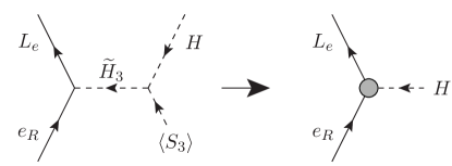
Figure 2: The Feynman diagram for generating the effective $e_{R}\mathchar 45\relax L_{e}\mathchar 45\relax H$ coupling after the SSB of gauged lepton number.

With one photon attached to the charged scalar in the loop diagrams shown in Fig.1, one can calculate the anomalous magnetic moments of electron and muon. For $m_{F}\gg m_{l}$, we have[44]

$$\triangle a_{e} = {\Re[y_{eR}^{*}\,y_{eL}]\over 32\pi^{2}}\frac{m_{e}}{M_{N}^{2}}\frac{\kappa_{3}v_{3}v_{0}}{M_{N}}{\cal\widetilde{I}}_{0}\left(\beta^{(e)}_{H},\beta^{(e)}_{L}\right)\,,$$

$$\triangle a_{\mu} = {\Re[y_{\mu R}^{*}\,y_{\mu L}]\over 32\pi^{2}}\frac{m_{\mu}}{M_{N}^{2}}\frac{\kappa_{5}v_{3}v_{0}}{M_{N}}{\cal\widetilde{I}}_{0}\left(\beta^{(\mu)}_{H},\beta^{(\mu)}_{L}\right)\,,$$ (14)

where $m_{e,\mu}$ are the physical lepton masses, and the loop function is given by

$${\cal\widetilde{I}}_{0}\equiv{{\cal J}_{0}(z_{1})-{\cal J}_{0}(z_{2})\over z_{1}-z_{2}}\,,\;\mbox{and}\;\;{\cal J}_{0}(z)={1-z^{2}+2z\ln z\over(z-1)^{3}}\,.$$ (15)

Note ${\cal\widetilde{I}}_{0}$ is symmetric and positively defined.

For electron and muon, the ratio

$$\frac{\triangle a_{l}}{m_{loop}^{(l)}}=\frac{m_{l}}{M_{N}^{2}}{\Re[y_{lR}^{*}\,y_{lL}]\over y_{lR}^{*}\,y_{lL}}{{\cal\widetilde{I}}_{0}\left(\beta^{(l)}_{H},\beta^{(l)}_{L}\right)\over{\cal F}_{0}\left(\beta^{(l)}_{H},\beta^{(l)}_{L}\right)}$$ (16)

is independent of the mixing angle, or equivalently $\kappa_{5,3}$. For muon, $y_{\mu R}^{*}\,y_{\mu L}$ can be made a real number by field redefinition or $m_{loop}^{(\mu)}=m_{\mu}\simeq 0.105\mathrm{GeV}$. Hence, $\triangle a_{\mu}>0$ follows and agrees with the sign of the measured $\triangle a_{\mu}^{B\!N\!L-F\!N\!A\!L}$. On the other hand, the tree-level Yukawa contribution mediated by $H_{3}$ is reserved for the electron, so either positive or negative $\triangle a_{e}$( $m_{loop}^{(e)}$) could be accommodated. Moreover, since $m_{\mu}$ is known, $\triangle a_{\mu}$ only depends on three physical masses, $M_{N}$ and $M^{(\mu)}_{H/L}$. In Fig.3 we display the allowed 2-dimensional parameter space of $M^{(\mu)}_{H/L}$, for a given $M_{N}$, which gives rise to the observed $1\sigma$ range of $\triangle a_{\mu}^{B\!N\!L-F\!N\!A\!L}$. As seen in Fig.3, the typical values for $M^{(\mu)}_{H/L}$ are about a few $\mathrm{TeV}$. We also show the product $y_{\mu R}^{*}y_{\mu L}s_{\alpha}^{(\mu)}c_{\alpha}^{(\mu)}$ vs $M_{N}$ in Fig.4. For a fixed $M_{N}$, we scan the region of $0.2\mathrm{TeV}<M_{L_{(\mu)}}<M_{H_{(\mu)}}<5\mathrm{TeV}$ to find the viable solution which yields the measured $\triangle a_{\mu}^{B\!N\!L-F\!N\!A\!L}$. The typical value of the mixing product is in the reasonable range of $10^{-2}-10^{-1}$ for $M_{N}\in[0.1,2.0]\mathrm{TeV}$, and the minimum, $\sim 10^{-2}$, happens at around $M_{N}\sim 1\mathrm{TeV}$. By assuming $|y_{\mu R,\mu L}|<\sqrt{4\pi}$, we obtain a lower bound $|\sin\alpha^{(\mu)}|\gtrsim 10^{-3}$ for $\triangle a_{\mu}^{B\!N\!L-F\!N\!A\!L}$, which is to be accommodated in this model.

It is evident that the new physics(NP) contribution to $\triangle a^{NP}_{\tau}=0$ at the 1-loop level. The leading contribution to $\triangle a^{NP}_{\tau}$ is the 2-loop Barr-Zee-like diagrams with charged scalars running in the loop, which gives rise to the effective $\gamma\gamma H_{SM}$ vertex. In this model, the charged scalars are $\phi_{H/L}^{(e,\mu)}$. The ballpark estimation gives

$$\triangle a^{NP}_{\tau}\sim\frac{\alpha_{em}}{(4\pi^{2})^{2}}\sum_{k}\frac{\mu_{k}}{v_{0}}\frac{m_{\tau}^{2}}{M_{k}^{2}}\ln\frac{M_{h}^{2}}{M_{k}^{2}}\,,$$ (17)

where $\mu_{k}$ represents the triple coupling of the charged scalar, of mass $M_{k}$, with the SM Higgs, and $M_{h}$ the SM Higgs mass. Taking $\mu_{k}\sim v_{0}$, $M_{k}\sim{\cal O}(\mathrm{TeV})$, this model predicts $|\triangle a^{NP}_{\tau}|\lesssim{\cal O}(10^{-10})$, which is beyond the experimental sensitivities in the near future.

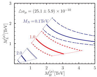
Figure 3: The 2-dimensional parameter space of $M_{H/L}$ for the muon. The solid(dash) lines represent $\triangle a_{\mu}$ at the central($1\sigma$ boundary) values for $M_{N}=\{0.1,1.0,2.0\}\mathrm{TeV}$.

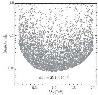
Figure 4: The mixing product $y_{\mu R}^{*}y_{\mu L}\sin\alpha^{\mu}\cos\alpha^{\mu}$ for muon v.s. $M_{N}$ for $\triangle a_{\mu}=25.1\times 10^{-10}$.

Now we turn our attention to the electron. Since one can only remove one physical CP phase through the field redefinition, it has to be reserved for making the physical mass real positive. Similar to the calculation of $\triangle a_{e}$, the electric dipole moment of the electron from NP can be derived as

$$d^{NP}_{e}=-e\frac{\Im[y_{eR}^{*}\,y_{eL}]}{64\pi^{2}}{\kappa_{3}v_{0}v_{3}\over M_{N}^{3}}{\cal\widetilde{I}}_{0}\left(\beta^{(e)}_{H},\beta^{(e)}_{L}\right)\,.$$ (18)

In terms of $\triangle a_{e}$, it can also be expressed as

$$d^{NP}_{e}=-{e\tan\delta^{(e)}_{CP}\over 2m_{e}}\triangle a_{e}\,,\;\mbox{where}\;\;\delta^{(e)}_{CP}={\rm{arg}}(y_{eR}^{*}\,y_{eL})\,.$$ (19)

Note that the $m_{e}$ here is the positive real physical mass. Plugging in the value of $\triangle a_{e}=-8.7[+4.8]\times 10^{-13}$ and the latest limit on $|d_{e}|<1.1\times 10^{-29}e\mathchar 45\relax cm$[45], we obtain a stringent bound that

$$\left|\tan\delta^{(e)}_{CP}\right|<6.56[3.62]\times 10^{-7}\,.$$ (20)

The phenomenological consideration indicates that the two phases of $m^{(e)}_{tree}$ and $m^{(e)}_{loop}$ are aligned to the level of ${\cal O}(10^{-7})$. The smallness of the relative phase, $\delta^{(e)}_{CP}$, cannot be addressed in the current model setup. It suggests that CP symmetry should be assumed, at least for the lepton sector. Therefore, in the rest of the paper, we set $\delta^{(e)}_{CP}=0$ for simplicity. Then, the overall phase can be removed by electron filed redefinition so

$$m_{e}=y^{(e)}_{tree}{v_{0}\over\sqrt{2}}+\triangle a_{e}\frac{M_{N}^{2}}{m_{e}}\widetilde{R}\left(\beta^{(e)}_{H},\beta^{(e)}_{L}\right)\,,\;\mbox{ where }\;\;\widetilde{R}(z_{1},z_{2})\equiv{{\cal F}_{0}\left(z_{1},z_{2}\right)\over{\cal\widetilde{I}}\left(z_{1},z_{2}\right)}\,$$ (21)

and $\widetilde{R}>0$. Equivalently, we have

$$y_{3}=\frac{6g_{l}}{\sqrt{2}}{M_{3}^{2}\over\mu_{H3}M_{X}}\left(1-\overline{R}_{e}\right)y^{(e)}_{SM}\,,\;\overline{R}_{e}\equiv\frac{m^{(e)}_{loop}}{m_{e}}=\triangle a_{e}\frac{M_{N}^{2}}{m_{e}^{2}}\widetilde{R}\left(\beta^{(e)}_{H},\beta^{(e)}_{L}\right)\,,$$ (22)

where $y^{(e)}_{SM}=\sqrt{2}m_{e}/v_{0}=2.94\times 10^{-6}$ is the SM electron Yukawa coupling. From Fig.5, we see the typical value of $|\overline{R}_{e}|$, the ratio of the radiative mass to the physical mass of electron, is about $\sim{\cal O}(10)$ for $M_{H,L}^{(e)}\sim\mathrm{TeV}$. If we take $M_{N}\simeq M_{X}\simeq 1\mathrm{TeV}$, $M_{3}(\sim M^{(\mu)}_{H})\simeq 2\mathrm{TeV}$, and $\overline{R}_{e}\simeq-10$, then

$$y^{Cs}_{3}\sim 1.497\times 10^{-2}\times\left({g_{l}\over 0.1e}\right)\times\left({10\mathrm{GeV}\over\mu_{H3}}\right)\,.$$ (23)

On the other hand, if one adopts $\triangle a_{e}^{Rb}=4.8\times 10^{-13}$ and keeps all other parameters fixed, then

$$y^{Rb}_{3}\sim-0.612\times 10^{-2}\times\left({g_{l}\over 0.1e}\right)\times\left({10\mathrm{GeV}\over\mu_{H3}}\right)\,.$$ (24)

Compared with $y^{(\tau)}_{SM}=1.02\times 10^{-2}$, this model does not need ridiculous fine tuning to yield the observed charged lepton mass hierarchy.

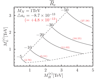
Figure 5: The contour (solid lines) plot of $\overline{R}_{e}=m^{(e)}_{loop}/m_{e}$, while the dashed lines indicate the boundary. We take the values $M_{N}=1$ TeV and $\triangle a^{Cs}_{e}=-8.7\times 10^{-13}$ as the reference. For different values of $\triangle a_{e}$, the contour values scale linearly in $\triangle a_{e}$. For example, the values in parentheses are for $\triangle a^{Rb}_{e}=+4.8\times 10^{-13}$.

III Charged lepton flavor violation

First, note that both the traditional lepton number and the accidental $Z_{\tau}$ parity are intact after the SSB of $U(1)_{\ell}$. If we follow the fermion line of an incoming tau for any Feynman diagram, it must end up with an outgoing tau. Therefore, there is no tau number violation in this model to all orders, and we only need to consider the CLFV in the electron and muon sectors. Because the SM gauge symmetries are at work in the intermediate energy scale between the SSB of $U(1)_{\ell}$ and the SSB of the SM electroweak, we address the possible CLFV in the $e-\mu$ sector by considering the SM gauge-invariant operators in terms of SM DOF.

Starting from dim-4, we need to consider only three operators (and their hermitian conjugations),

$$\overline{L}_{\mu}\gamma^{\alpha}D_{\alpha}L_{e}\,,\;\overline{\mu}_{R}\gamma^{\alpha}D_{\alpha}e_{R}\,,\;\overline{L}_{\mu}e_{R}H\,,$$ (25)

where $D_{\alpha}$ is the SM covariant derivative. The first two operators give rise to the CLFV wavefunction corrections, while the last one generates the cross-flavor mass term below the SSB of SM electroweak. The most general Feynman diagrams consist of two external leptons can be pictorially illustrated in Fig.6(a,b), where the gray blobs represent any possible perturbative Feynman diagrams that constitute the vertices.

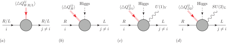
Figure 6: The dim-4 (a,b) and the dim-6 (c,d) dipole charged lepton flavor changing operators and the required quantum number injection (double line). The gray blobs represent any possible perturbative Feynman diagrams that constitute the vertices. The indices $i,j$ stand for flavor and $L/R$ label the charged lepton chirality.

The corresponding $U(1)_{\ell}$ charges for operators listed in Eq.(25) are $\{-8,-14,-11\}$, respectively. In this model, only $H$ and $S_{3}$ are higgsed, thus the injected $U(1)_{\ell}$ charge can only be $\triangle Q_{l}=3k$, where $k$ is an integer, corresponding to the number of external $S_{3}$ lines above the SSB of $U(1)_{\ell}$. Therefore, all the dim-4 CLFV operators are forbidden to all orders in this model. And the resulting $h_{SM}\rightarrow\mu e$ from the dim-4 operators also vanishes.

We move on to consider the dim-6 operators. The complete SM gauge-invariant dimension-6 dipole, Fig.6(c,d), and 4-lepton operators, Fig.7, are

$$\widetilde{O}_{D1}^{ij}=\left(\overline{L}_{i}\sigma^{\alpha\beta}R_{j}\right)HF_{\alpha\beta}\,,\;\widetilde{O}_{D2}^{ij}=\left(\overline{L}_{i}\sigma^{\alpha\beta}\overrightarrow{\tau}R_{j}\right)H\overrightarrow{W}_{\alpha\beta}\,,$$

$$\widetilde{O}_{LL}^{ijab}=\left(\overline{L}_{i}\gamma^{\alpha}L_{j}\right)\left(\overline{L}_{a}\gamma^{\alpha}L_{b}\right)\,,\,\widetilde{O}_{LR}^{ijab}=\left(\overline{L}_{i}\gamma^{\alpha}L_{j}\right)\left(\overline{R}_{a}\gamma^{\alpha}R_{b}\right)\,,\,\widetilde{O}_{RR}^{ijab}=\left(\overline{R}_{i}\gamma^{\alpha}R_{j}\right)\left(\overline{R}_{a}\gamma^{\alpha}R_{b}\right)\,,$$ (26)

where $\vec{\tau}$ is the Pauli matrix, $F_{\alpha\beta}$ and $W_{\alpha\beta}$ are the field strengthes of $U(1)_{Y}$ and $SU(2)_{L}$, respectively. The operators $\widetilde{O}_{D1,D2}^{\mu e}$ need $+11$ $U(1)_{\ell}$ charge injection and are forbidden to all orders. As a result, the dimension-6 contributions to $\mu\rightarrow e\gamma$ and $Z\rightarrow\mu e$ vanish.

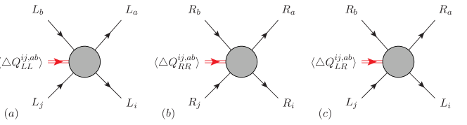
Figure 7: The general Feynman diagrams for the CLVF 4-lepton operators and the required quantum number injection(double line). The gray blobs represent any possible perturbative Feynman diagrams that constitute the vertices.The indices $i,j,a,b$ stand for flavor, and $L/R$ label the charged lepton chirality.

For the CLFV 4-lepton operators, the required quantum numbers injection ( double line in Fig.7 ) into these blobs are listed in Table 4, where the $(e\mu)(ee)$ column relates to $\mu\rightarrow 3e$, and the $(e\mu)(e\mu)$ column relates to muonium-antimuonium oscillations. Again, only $H$ and $S_{3}$ are higgsed in this model, and none of the required quantum number injection is possible to all orders. One can easily generalize the analysis to the dim-6 2-lepton-2-quark operators and conclude there is no CLFV 4-fermion operator to all orders in this model setup. The dim-6 operator for $\mu\mathchar 45\relax e$ conversion on nuclei is also forbidden.

operator $\diagdown$ (ij)(ab)	$(e\mu)(l_{k}l_{k})$	$(e\mu)(e\mu)$	$(\tau e)(\mu\tau)$
$\widetilde{O}_{LL}^{ijab}$	$8$	$16$	$-8$
$\widetilde{O}_{RR}^{ijab}$	$14$	$28$	$-14$
$\widetilde{O}_{LR}^{ijab}$	$8$	$22$	$-11$
$\widetilde{O}_{RL}^{ijab}$	$14$	$22$	$-11$

Table 4: The net $U(1)_{\ell}$ charge of the CLFV dimension-six 4-lepton operators, where $l_{k}=e,\mu,\tau$, and $i,j,a,b$ are the flavor indices.

In principle, the RGE evolution could induce CLFV below the electroweak scale from higher dimensional($>6$) operators. Although the general discussion on CLFV operators with dimensions higher than six is beyond the scope of this paper, we expect the RGE running effects to be suppressed and insignificant.

IV Phenomenology

By convention, we will take $g_{2},g_{1},g_{l}$, the gauge coupling strengths, to be positive. Since the SM parts in the covariant derivative

$$D_{\mu}=\partial_{\mu}-ig_{2}|T_{3}|\,\vec{\sigma}\cdot\vec{A}_{\mu}-ig_{1}YB_{\mu}-ig_{l}Q_{l}X_{\mu}$$ (27)

stay the same, we focus on the new gauge $U(1)_{l}$ interaction part. The leptons interact with the new gauge boson $X$ via

$${\cal L}\supset-ig_{l}\sum_{l}\left[\bar{l}\gamma_{\mu}(G_{lL}\hat{L}+G_{lR}\hat{R})l\right]X^{\mu}$$ (28)

with $-G_{eL}=G_{\mu L}=4$, $-G_{eR}=G_{\mu R}=7$, and $G_{\tau L}=G_{\tau R}=0$.

If integrating out the heavy $X$, one obtains an effective contact interaction $\frac{16g_{l}^{2}}{M_{X}^{2}}(\bar{e}_{L}\gamma^{\alpha}e_{L})(\bar{\mu}_{L}\gamma_{\alpha}\mu_{L})$. From the limit[10] $\Lambda^{+}(ee\mu\mu)>8.5\mathrm{TeV}$, we get

$$g_{l}<\sqrt{\frac{\pi}{8}}\left({M_{X}\over 8.5\mathrm{TeV}}\right)\simeq 0.24e\left({M_{X}\over\mathrm{TeV}}\right)\,.$$ (29)

The widthes of $X$ decays into fermion and scalar pairs are given by

$$\Gamma_{X\rightarrow l^{+}l^{-}} = \Theta(1-4\beta_{l})\frac{g_{l}^{2}}{24\pi}M_{X}[G_{lL}^{2}+G^{2}_{lR}+6\beta_{f}G_{lL}G_{lR}]\sqrt{1-4\beta_{l}}\,,$$ (30)

$$\Gamma_{X\rightarrow SS^{*}} = \Theta(1-4\beta_{S})\frac{g_{l}^{2}Q_{s}^{2}}{48\pi}M_{X}(1-4\beta_{S})^{\frac{3}{2}}\,,$$ (31)

respectively. In the above, $Q_{s}$ is the $U(1)_{\ell}$ charge of the scalar $S$, $\beta_{i}=(m_{i}/M_{X})^{2}$, and $\Theta$ is the step function. If all the exotic scalars are heavier than $M_{X}/2$, the decay width of $X$ is dominated by the modes with 2-body $e^{+}e^{-},\mu^{+}\mu^{-},\bar{\nu}_{e}{\nu}_{e},\bar{\nu}_{\mu}{\nu}_{\mu}$ final states. One has

$${\Gamma_{X}\over M_{X}}\simeq 27\alpha_{em}\left(\frac{g_{l}}{e}\right)^{2}<1.17\times 10^{-2}\left({M_{X}\over\mathrm{TeV}}\right)^{2}\,,$$ (32)

where $\alpha_{em}$ is the fine structure constant, and the upper bound stems from Eq.(29). At the $X$-pole, the narrow-width gauge boson has a large cross-section

$$\sigma(e^{+}e^{-}\rightarrow X^{*}\rightarrow l^{+}l^{-})={g_{l}^{4}(G^{2}_{eL}+G^{2}_{eR})^{2}\over 24\pi M_{X}^{2}}\frac{M_{X}^{2}}{\Gamma_{X}^{2}}\,,$$ (33)

where $l=e,\mu$. For $M_{X}=1\mathrm{TeV}$ and $g_{l}=0.1e$, this cross-section is about $6.1\times 10^{10}\,fb$. If $X$ boson can be produced at the future high energy $e^{+}e^{-}$ collider, the narrow peaks of invariant masses $m_{ee}\sim m_{\mu\mu}\sim M_{X}$ will be smoking gun evidence of the gauge $U(1)_{\ell}$. On the other hand, even below the $X$ resonance, the interferences between $X$ and the SM gauge boson cause significant differences in the forward-backward asymmetry of leptons. The formulae of forward-backward asymmetry of leptons have been collected in Appendix C. In Fig.8, we display the $A_{FB}$ of three leptons by assuming that $M_{X}=1\mathrm{TeV}$, $g_{l}=0.1e$, $Q_{l}^{N}=-1$, and $X$ only decays into a lepton pair. Since tauon does not couple to $X$, it follows the SM prediction. Due to the different $U(1)_{l}$ charges, $A^{e}_{FB}$ and $A^{\mu}_{FB}$ differ from the SM prediction significantly. At the Z-pole, $A^{e}_{FB}/A^{\tau}_{FB}\sim 1.0001$ and $A^{\mu}_{FB}/A^{\tau}_{FB}\sim 0.9999$. However, the current experimental precision cannot tell the differences at $Z$-pole. The differences grow and reach $\sim{\cal O}(1)$ as $\sqrt{s}$ increases and approaches $M_{X}$. This prediction is robust and can be tested by future $e^{+}e^{-}$ colliders.

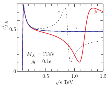
Figure 8: Lepton forward-backward asymmetry for $M_{X}=1\mathrm{TeV}$, $g_{l}=0.1e$, and $Q_{l}^{N}=-1$. If one adopts the other $U(1)_{l}$ charge assignment with the signs of all $U(1)_{\ell}$ charges flipped, then $A^{e}_{FB}\Leftrightarrow A^{\mu}_{FB}$.

It is well-known that the oblique parameters[47] $S$ and $T$ constrain the mass splitting of the doublet scalars. In this model, $H_{5}$ and $H_{3}$ contribute

$$\triangle T_{i}=\frac{1}{16\pi s_{W}^{2}}\frac{M_{i+}^{2}}{M_{W}^{2}}\left[1+z_{i}+{2z_{i}\over 1-z_{i}}\ln z_{i}\right]\,,\;\triangle S_{i}=-\frac{1}{12\pi}\ln z_{i}\,,\;\;(i=H_{5},H_{3})\,,$$ (34)

where $z_{i}=(M_{i-}/M_{i+})^{2}$ is the ratio of $T_{3}=-1/2$ charged component mass squared to that of the $T_{3}=1/2$ neutral component. Expanding around the degenerate case and denote $\triangle M_{i}=M_{i+}-M_{i-}$,

$$\triangle T_{i}\simeq\frac{1}{12\pi s_{W}^{2}}\frac{(\triangle M_{i})^{2}}{M_{W}^{2}}\,,\;\triangle S_{i}\simeq\frac{1}{6\pi}\frac{\triangle M_{i}}{M_{i+}}\,.$$ (35)

$\triangle S_{i}$ can be either positive or negative, but $\triangle T_{i}$ is always positive. Thus, without any sign ambiguity, $\triangle T=\triangle T_{5}+\triangle T_{3}$ can be used to constrain the model parameters. From $T_{exp}<0.22$ at $95\%$ C.L.[10],

$$\triangle M_{5}^{2}+\triangle M_{3}^{2}<1.91M_{W}^{2}\,.$$ (36)

Compared to $M_{5},M_{3}\sim{\cal O}(\mathrm{TeV})$, both $H_{5}$ and $H_{3}$ have small mass splitting, $\lesssim M_{W}$. This implies that $\tilde{\lambda}_{H3/H5}\simeq\bar{\lambda}_{H3/H5}$ and $|\kappa_{5,3}|<1$ so that the mixings between $H_{5,3}$ and other scalars are small.

IV.1 Effective Yukawa couplings

The loop-induced $h_{SM}\bar{e}e$ vertex yields an effective Yukawa coupling. Together with the tree-level contribution, the resulting effective electron-Higgs Yukawa coupling is the sum of two. We take the ratio to the SM electron-(125$\mathrm{GeV}$ Higgs) Yukawa, $y^{e}_{SM}=m_{e}/v_{0}$, and define the normalized electron-Higgs Yukawa as

$$\zeta_{e}={y^{(e)}_{eff}\over y^{e}_{SM}}=1+\overline{R}_{e}\times\left\{-1+A_{0}\!+\!\left[s_{2}^{2}-c_{2}\left(\lambda_{H3}\!+\!\tilde{\lambda}_{H3}\!-\!\lambda_{H6}\right)\!B_{1}\right]\!A_{1}+(\lambda_{H3}\!+\!\tilde{\lambda}_{H3}\!+\!\lambda_{H6})\!B_{1}A_{2}\right\}\,.$$ (37)

In the above, the short-handed notations represent

$$s_{2} = \sin(2\alpha^{(e)})\,,\;c_{2}=\cos(2\alpha^{(e)})\,,\;B_{1}=\frac{v_{0}^{2}}{M_{N}^{2}}{1\over(z_{H}-z_{L})}\,,$$

$$A_{0} = {{\cal F}\left(z_{L},z_{H},z_{h}\right)\over{\cal F}_{0}\left(z_{L},z_{H}\right)}\,,$$

$$A_{1} = {{\cal F}\left(z_{H},z_{H},z_{h}\right)+{\cal F}\left(z_{L},z_{L},z_{h}\right)-2{\cal F}\left(z_{L},z_{H},z_{h}\right)\over 2{\cal F}_{0}\left(z_{L},z_{H}\right)}\,,$$

$$A_{2} = {{\cal F}\left(z_{H},z_{H},z_{h}\right)-{\cal F}\left(z_{L},z_{L},z_{h}\right)\over 2{\cal F}_{0}\left(z_{L},z_{H}\right)}\,,$$ (38)

where $z_{H}=(M^{(e)}_{H}/M_{N})^{2}$, $z_{L}=(M^{(e)}_{L}/M_{N})^{2}$, $z_{h}=(q_{h}^{2}/M_{N}^{2})$, and $q_{h}$ is the 4-momentum carried by the SM Higgs. Numerically, the $z_{h}$ contribution is insignificant, see Appendix B, $A_{0}=1+{\cal O}(10^{-3})$, $A_{1}>0$, $A_{2}<0$, and the absolute values of $A_{1,2}$ increase as the ratio $z_{H}/z_{L}$ gets bigger. We illustrate the normalized electron-Higgs Yukawa for one particular set of parameters in Fig.9. One can see that the electron-Higgs Yukawa can be very different, both in magnitude and sign, from the SM prediction.

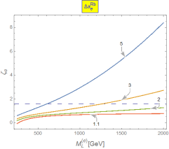
Figure 9: The normalized electron-Higgs Yukawa $\zeta_{\mu}$ vs $M_{L}^{(e)}$ for $M_{H}^{(e)}/M_{L}^{(e)}=\{1.1,2,3,5\}$. Here we set $M_{N}=1\mathrm{TeV}$, $\sin(2\alpha^{(e)})=0.3$, $q_{h}^{2}=(125\mathrm{GeV})^{2}$, and $\lambda_{H3}=\tilde{\lambda}_{H3}=\lambda_{H6}=1.0$. The horizontal dashed lines indicate the future experimental sensitivity, $|\zeta_{e}|<1.6$ at FCC-ee[15].

To better explore this model, we perform a numerical scan with $0.2\mathrm{TeV}<M_{L}<M_{H}<10\mathrm{TeV}$, $\sin(2\alpha^{(e)})\in[-.3,+.3]$, and each $\lambda_{H3},\tilde{\lambda}_{H3},\lambda_{H6}\in[0.1,\sqrt{4\pi}]$. The histogram of the resulting $\zeta_{e}$ is displayed in Fig.10, where the vertical dashed lines indicate the projected sensitivity, $|\zeta_{e}|<1.6$ at $95\%$ CL, at FCC-ee[15]. With the projected sensitivity at the FCC-ee, about $40.6(12.6)\%$ of $\zeta_{e}$ for $\triangle a_{e}^{Cs(Rb)}$ can be detected. If adopting $\triangle a_{e}^{Cs}$, $\zeta_{e}$ spans from $-33.1$ to $5.4$ and peaks in the range $[1.0,2.0](\sim 70\%)$. The probability for $\{\zeta_{e}<-5\,,\;\zeta_{e}<-3\,,\;\zeta_{e}>3\}$ are $\{2.3\%,4.1\%,0.45\%\}$, respectively. On the other hand, if $\triangle a_{e}^{Rb}$ is adopted, $\zeta_{e}$ spans from $-1.4$ to $19.8$ and peaks around $[0.5,1.0](\sim 67\%)$. The chances for $\{\zeta_{e}>5,\zeta_{e}>3,\zeta_{e}<-1\}$ are $\{1.6\%,4.7\%,2\times 10^{-4}\}$, respectively. From the scan, we see that the abnormal electron-Higgs coupling is possible to be tested in the near future.

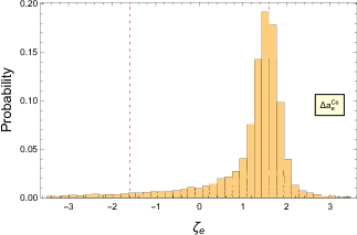
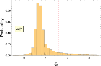
Figure 10: The histogram of the normalized electron-Higgs Yukawa $\zeta_{e}$. The vertical dashed lines indicate the future experimental sensitivity, $|\zeta_{e}|<1.6$ at FCC-ee[15].

On the other hand, muon receives only the radiative mass correction such that $\overline{R}_{\mu}=1$. In Fig.11, we display the normalized muon-Higgs Yukawa for a particular parameter set $\sin(2\alpha^{(\mu)})=0.1$ and $\lambda_{H5}=\tilde{\lambda}_{H5}=\lambda_{H8}=\lambda_{\mu}$. The effective muon-Higgs Yukawa is close to the SM one when $\lambda_{\mu}=0.1$. If one adopts a larger coupling $\lambda_{\mu}$, $\zeta_{\mu}<1$, it could be as small as $\sim 0.4$ when $\lambda_{\mu}=3$ and $M_{N}=2\mathrm{TeV}$.

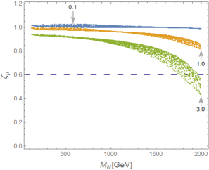
Figure 11: The normalized muon-Higgs Yukawa $\zeta_{\mu}$ vs $M_{N}$. Here we set $\triangle a_{\mu}=25.1\times 10^{-10}$, $\sin(2\alpha^{(\mu)})=0.1$, and $\lambda_{H5}=\tilde{\lambda}_{H5}=\lambda_{H8}=\{0.1,1.0,3.0\}$. The horizontal dashed line is the current experimental lower limit on $\zeta_{\mu}>0.6$[6, 7].

It usually stays within the current $2\sigma$ constraint, $0.6\lesssim\zeta_{\mu}\lesssim 1.5$[6, 7]. We also perform a numerical scan over the ranges: $M_{N}\in[0.2,2.0]\mathrm{TeV}$, $\sin(2\alpha^{\mu})\in[-0.3,0.3]$, and each $\lambda_{H5},\tilde{\lambda}_{H5},\lambda_{H8}\in[0.1,\sqrt{4\pi}]$. The histogram of the resulting $\zeta_{\mu}$ is shown in Fig.12. The normalized muon Yukawa spans from $0.38$ to $1.21$ and mostly peaks in the range of $[0.8,1.0](\sim 82.0\%)$, with the chance of $\sim 7.5\%(0.66\%)$, for $\zeta_{\mu}$ being greater than $1.0$ (or smaller than the current lower bound $0.6$).

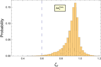
Figure 12: The histogram of the normalized muon-Higgs Yukawa $\zeta_{\mu}$. The vertical dashed line indicates the current experimental lower limit on $\zeta_{\mu}>0.6$ [6, 7].

See [11] for the future updates of $\zeta_{\mu}$ at HL-LHC and $e^{+}e^{-}$ colliders. With the ultima projected precision of $\sim 0.4\%$ at the future FCC[12], the entire range of predicted muon-Yukawa can be covered and probed.

V Dark matter and neutrino masses

The current model does not have a dark matter ( DM ) candidate. However, with the gauged $U(1)_{\ell}$ symmetry, DM candidate can be easily included by extending the particle content. One can introduce a pair of vector fermion $D$ which only interacts with the gauge boson $X$ by adjusting its $U(1)_{\ell}$ charge, $Q_{D}$. Then $D$ can be assigned with a dark parity without upsetting any gauge symmetry. This dark parity remains even after the SSB of $U(1)_{\ell}$ and SM electroweak, making $D$ a DM candidate. The annihilation cross section of $D\bar{D}\rightarrow X^{*}\rightarrow f\bar{f}$ can be calculated to be

$$\left\langle\sigma v\right\rangle_{D\bar{D}\rightarrow f\bar{f}}\simeq Q_{D}^{2}g_{l}^{4}{(G_{L}^{f})^{2}+(G_{R}^{f})^{2}\over\sqrt{2}\pi M_{X}^{2}}{\beta_{D}\over(1-4\beta_{D})^{2}}\,,$$ (39)

where $\beta_{D}=(M_{D}/M_{X})^{2}$. Since the third generation lepton is $U(1)_{l}$ neutral, the final states can be $l^{+}l^{-}$ or $\bar{\nu}_{l}\nu_{l}$ and $l=e,\mu$. From $\Omega_{DM}h^{2}=0.120\pm 0.001$[48] and $\Omega_{DM}h^{2}\simeq 4.8\times 10^{-10}(\mathrm{GeV})^{-2}/\langle\sigma v\rangle$, we obtain

$$\left(\frac{Q_{D}}{10}\right)^{2}\left(\frac{g_{l}}{e}\right)^{4}\frac{1}{M_{X}^{2}}{\beta_{D}\over(1-4\beta_{D})^{2}}\simeq 1.1\times 10^{-10}(\mathrm{GeV})^{-2}\,.$$ (40)

For $M_{X}=1\mathrm{TeV}$, $Q_{D}=10$, and $g_{l}=0.1e$, either $M_{D}=0.394\mathrm{TeV}$ or $M_{D}=0.633\mathrm{TeV}$ can yield the correct DM relic density. Moreover, since $D$ is leptophilic, it can safely escape the direct search bound.

Finally, we comment on how to generate the active neutrino masses in this model. The Majorana neutrino mass matrix element ${\cal M}^{\nu}_{ij}$ can arise from the corresponding Weinberg operator[49] $(L_{i}H)(L_{j}H)$. However, the traditional lepton number is conserved in the current model, which forbids the Weinberg operator. One possible simple extension is introducing an extra $U(1)_{\ell}$ charge-2 scalar $S_{2}$ and allowing it to develop VEV. Therefor, the $U(1)_{l}$ charge of every Weinberg operator can be balanced, and the observed neutrino oscillation data can be explained at the price of potential CLFV. In that case, one must carefully consider the stringent CLFV constraints ( see [43], for example), and the comprehensive analysis is beyond the scope of this paper.

VI Conclusion

We have proposed an anomaly-free gauged lepton number $U(1)_{\ell}$ symmetry where the observed $\triangle a_{e,\mu}$ are explained, and the charged lepton mass hierarchy arises naturally. On top of the SM particle content, this model requires one pair of vector fermions, two scalar doublets, and three scalar singlets, see Table 2, with TeV-ish masses. The flavor-dependent $U(1)_{\ell}$ charge assignment, see Table 1, is novel to our best knowledge. In our model, tau picks up its mass via the SM Yukawa interaction, while the $U(1)_{\ell}$ charge assignment forbids the SM Yukawa interactions for electron and muon. Both electron and muon acquire a radiatively generated mass from the photon-removed one-loop diagrams for the observed $\triangle a_{e,\mu}$. Electron receives an extra mass contribution from its coupling to SM Higgs mediated by one of the exotic doublet scalars. Compared to the SM tau Yukawa coupling, this model does not require extreme model parameters to reproduce the observed $m_{e,\mu}$ and $\triangle a_{e,\mu}$.

This model has two nice features: (1) either positive $\triangle a_{e}^{Rb}\simeq 4.8\times 10^{-13}$[37] or negative $\triangle a_{e}^{Cs}\simeq-8.7\times 10^{-13}$[36] can be accommodated with $\triangle a_{\mu}^{B\!N\!L-F\!N\!A\!L}\simeq 25.1\times 10^{-10}$[30] in this model, and (2) without any ad hoc symmetries or parities introduced, the automatically emerged conventional lepton number and tau-parity ensure that the tau flavor is conserved to all orders in this model. We have also proved that in the $e-\mu$ sector, all the dim-4 and dim-6 CLFV SM operators vanish to all orders. Hence, no CLFV constraint on this model is expected in the foreseeable future.

We have discussed the phenomenology and pointed out two testable signatures of this model: (1) depending on the overall sign of $U(1)_{\ell}$ charges, we predicted either $A_{FB}^{e}>A_{FB}^{\tau}>A_{FB}^{\mu}$ or $A_{FB}^{e}<A_{FB}^{\tau}<A_{FB}^{\mu}$. This can be tested at the future $e^{+}e^{-}$ colliders before the direct discovery of the $U(1)_{\ell}$ gauge boson. (2) The abnormal electron- and muon-Higgs Yukawa couplings. Our numerical study found that $-33\lesssim y^{(e)}_{eff}/y^{e}_{SM}\lesssim 20$ and $0.6\lesssim y^{(\mu)}_{eff}/y^{\mu}_{SM}\lesssim 1.2$, which could be probed in the HL-LHC or future $e^{+}e^{-}$ colliders.

Finally, this simple model with this specific $U(1)_{\ell}$ charge assignment can be ruled out if: (1) any tau flavor violation is confirmed or (2) $|\triangle a_{\tau}|>10^{-10}$ is observed.

Appendix A Scalar sector

Here we spell out the most general scalar sector lagrangian for this model. The relevant lagrangian can be written as

$${\cal L}\supset{\cal L}_{1}-V_{1}-V_{2}\,.$$ (41)

The kinetic and quadratic terms are collected in ${\cal L}_{1}$:

$${\cal L}_{1} = (D_{\mu}H)^{\dagger}(D^{\mu}H)+(D_{\mu}H_{5})^{\dagger}(D^{\mu}H_{5})+(D_{\mu}H_{3})^{\dagger}(D^{\mu}H_{3})$$ (42)

$$+ (D_{\mu}C_{6})^{\dagger}(D^{\mu}C_{6})+(D_{\mu}C_{8})^{\dagger}(D^{\mu}C_{8})+(D_{\mu}S_{3})^{\dagger}(D^{\mu}S_{3})$$

$$+ \mu^{2}H^{\dagger}H-M_{5}^{2}H_{5}^{\dagger}H_{5}-M_{3}^{2}H_{3}^{\dagger}H_{3}-M^{2}_{6}|C_{6}|^{2}-M_{8}^{2}|C_{8}|^{2}+\mu_{l}^{2}|S_{3}|^{2}\,,$$

where the covariant derivative is

$$D_{\mu}=\partial_{\mu}-ig_{2}|T_{3}|\,\vec{\sigma}\cdot\vec{A}_{\mu}-ig_{1}YB_{\mu}-ig_{l}Q_{l}X_{\mu}\,.$$ (43)

The gauge invariant renormalizable quartic coupling potential is

$$V_{1} = \lambda_{H}(H^{\dagger}H)^{2}+\lambda_{H5}(H^{\dagger}H)(H_{5}^{\dagger}H_{5})+\lambda_{H3}(H^{\dagger}H)(H_{3}^{\dagger}H_{3})+\lambda_{H6}(H^{\dagger}H)|C_{6}|^{2}+\lambda_{H8}(H^{\dagger}H)|C_{8}|^{2}$$ (44)

$$+ \lambda_{Hl}(H^{\dagger}H)|S_{3}|^{2}+\lambda_{5}(H_{5}^{\dagger}H_{5})^{2}+\lambda_{53}(H_{5}^{\dagger}H_{5})(H_{3}^{\dagger}H_{3})+\lambda_{56}(H_{5}^{\dagger}H_{5})|C_{6}|^{2}+\lambda_{58}(H_{5}^{\dagger}H_{5})|C_{8}|^{2}$$

$$+ \lambda_{5l}(H_{5}^{\dagger}H_{5})|S_{3}|^{2}+\lambda_{3}(H_{3}^{\dagger}H_{3})^{2}+\lambda_{36}(H_{3}^{\dagger}H_{3})|C_{6}|^{2}+\lambda_{38}(H_{3}^{\dagger}H_{3})|C_{8}|^{2}+\lambda_{3l}(H_{3}^{\dagger}H_{3})|S_{3}|^{2}$$

$$+ \lambda_{6}|C_{6}|^{4}+\lambda_{68}|C_{6}|^{2}|C_{8}|^{2}+\lambda_{6l}|C_{6}|^{2}|S_{3}|^{2}+\lambda_{8}|C_{8}|^{4}+\lambda_{8l}|C_{8}|^{2}|S_{3}|^{2}+\lambda_{l}|S_{3}|^{4}$$

$$+ \widetilde{\lambda}_{H5}(H^{\dagger}H_{5})(H_{5}^{\dagger}H)+\widetilde{\lambda}_{H3}(H^{\dagger}H_{3})(H_{3}^{\dagger}H)+\widetilde{\lambda}_{53}(H_{5}^{\dagger}H_{3})(H_{3}^{\dagger}H_{5})$$

$$+ \bar{\lambda}_{H5}(H^{\dagger}\widetilde{H}_{5})(\widetilde{H}_{5}^{\dagger}H)+\bar{\lambda}_{H3}(H^{\dagger}\widetilde{H}_{3})(\widetilde{H}_{3}^{\dagger}H)+\bar{\lambda}_{53}(H_{5}^{\dagger}\widetilde{H}_{3})(\widetilde{H}_{3}^{\dagger}H_{5})\,.$$

Also, we have

$$V_{2}=\mu_{H3}H^{\dagger}\widetilde{H}_{3}S^{*}_{3}+\kappa_{3}H^{\dagger}H_{3}S_{3}^{*}C_{6}+\kappa_{5}H^{\dagger}H_{5}S_{3}C_{8}+H.c.$$ (45)

From the above, the mass matrix for the charged scalars after SSB can be read

$${\cal L}\supset-(H_{3}^{+},C_{6}^{+}){\cal M}_{36}\left(\begin{array}[]{c}H_{3}^{-}\\ C_{6}^{-}\\ \end{array}\right)-(H_{5}^{+},C_{8}^{+}){\cal M}_{58}\left(\begin{array}[]{c}H_{5}^{-}\\ C_{8}^{-}\\ \end{array}\right)\,,$$ (46)

where

$${\cal M}_{36}=\left(\begin{array}[]{cc}M_{3}^{2}+\frac{\lambda_{H3}+\widetilde{\lambda}_{H3}}{2}v_{0}^{2}+\frac{\lambda_{3l}}{2}v_{3}^{2}&\frac{1}{2}\kappa_{3}v_{0}v_{3}\\ \frac{1}{2}\kappa_{3}v_{0}v_{3}&M_{6}^{2}+\frac{\lambda_{H6}}{2}v_{0}^{2}+\frac{\lambda_{6l}}{2}v_{3}^{2}\\ \end{array}\right)\,,$$ (47)

and a similar form for ${\cal M}_{58}$. Also, the couplings between the charged scalars and the neutral component of the SM Higgs doublet $h$ is

$${\cal L}\supset-h(H_{3}^{+},C_{6}^{+})\Lambda_{36}\left(\begin{array}[]{c}H_{3}^{-}\\ C_{6}^{-}\\ \end{array}\right)\,,\;\;\Lambda_{36}=\left(\begin{array}[]{cc}(\lambda_{H3}+\widetilde{\lambda}_{H3})v_{0}&\frac{1}{2}\kappa_{3}v_{3}\\ \frac{1}{2}\kappa_{3}v_{3}&\lambda_{H6}v_{0}\\ \end{array}\right)\,.$$ (48)

Appendix B 1-loop function

When evaluating the Feynman diagrams displayed in Fig.1, one encounters the following integral

$${\cal F}(a,b,c)=\int_{0}^{1}dx\int^{1-x}_{0}dy{1\over 1-x-y+ax+by-xyc}\,,$$ (49)

where $a,b,c\geq 0$. As long as $c<4\sqrt{ab}$, ${\cal F}(a,b,c)$ is always positive. For $c\ll a,b$, the loop integral can be expanded as

$${\cal F}(a,b,c)={\cal F}_{0}(a,b)+c\,{\cal F}_{1}(a,b)+{\cal O}(c^{2})\,,$$ (50)

where

$${\cal F}_{0}(a,b) = \frac{1}{a-b}\left(\frac{a\ln a}{a-1}-\frac{b\ln b}{b-1}\right)\,,$$

$${\cal F}_{1}(a,b) = \int_{0}^{1}dx\int^{1-x}_{0}dy{xy\over(1-x-y+ax+by)^{2}}\,.$$ (51)

For the parameter space we are interested in, $0.2\,\mathrm{TeV}<M_{N}<2\,\mathrm{TeV}$ and $0.5\,\mathrm{TeV}<M_{L_{l}}<M_{H_{l}}<\,10\mathrm{TeV}$, $10^{-5}<{\cal F}_{1}/{\cal F}_{0}<0.5$. Moreover,

$${\cal F}_{0}(a,b)\rightarrow{a-1-\ln a\over(a-1)^{2}}\,,\;\;\mbox{when }a\rightarrow b\,.$$ (52)

Appendix C Forward-backward asymmetry

The tree level forward-backward asymmetry of $e^{+}e^{-}\rightarrow f\bar{f}$ due to the interference among photon, $Z$, and $X$ can be easily calculated and summarized as

$$A^{f}_{FB}(s) \equiv {\sigma^{F}(e^{+}e^{-}\rightarrow f\bar{f})-\sigma^{B}(e^{+}e^{-}\rightarrow f\bar{f})\over\sigma^{F}(e^{+}e^{-}\rightarrow f\bar{f})+\sigma^{B}(e^{+}e^{-}\rightarrow f\bar{f})}$$ (53)

$$= \frac{3}{4}{\sum_{a,b=\gamma,Z,X}K_{ab}(s)(L_{ab}^{e}-R_{ab}^{e})(L_{ab}^{f}-R_{ab}^{f})\over\sum_{a,b=\gamma,Z,X}K_{ab}(s)(L_{ab}^{e}+R_{ab}^{e})(L_{ab}^{f}+R_{ab}^{f})}\,.$$

The interfering terms are given by

$$K_{ab}(s)=(2-\delta_{ab})\Re\left[\left(1-\frac{M^{2}_{a}}{s}+i\frac{M_{a}\Gamma_{a}}{s}\right)^{-1}\left(1-\frac{M^{2}_{b}}{s}-i\frac{M_{b}\Gamma_{b}}{s}\right)^{-1}\right]\,,$$ (54)

where $s$ is the CM energy squared, and the Kronecker delta function takes care of the proper factors. The short handed notations are defined as

$$L^{f}_{ab}=G^{f}_{aL}G^{f}_{bL}\,,\;R^{f}_{ab}=G^{f}_{aR}G^{f}_{bR}\,,$$ (55)

where $G_{L/R}$ is the gauge couplings normalized to $e$. Namely, $G^{f}_{\gamma,L/R}=Q^{f}$, $G^{f}_{Z,L/R}=(T_{3}-Q)^{f}_{L/R}/(c_{W}s_{W})$, and $G^{f}_{X,L/R}=(g_{l}/e)Q^{f}_{lL/R}$.

References

- Aaboud et al. [2018a] M. Aaboud et al. (ATLAS), Measurements of Higgs boson properties in the diphoton decay channel with 36 fb-1 of collision data at TeV with the ATLAS detector, Phys. Rev. D 98, 052005 (2018a), arXiv:1802.04146 [hep-ex] .
- Aaboud et al. [2018b] M. Aaboud et al. (ATLAS), Observation of decays and production with the ATLAS detector, Phys. Lett. B 786, 59 (2018b), arXiv:1808.08238 [hep-ex] .
- Sirunyan et al. [2018a] A. M. Sirunyan et al. (CMS), Observation of Higgs boson decay to bottom quarks, Phys. Rev. Lett. 121, 121801 (2018a), arXiv:1808.08242 [hep-ex] .
- Aad et al. [2015] G. Aad et al. (ATLAS), Evidence for the Higgs-boson Yukawa coupling to tau leptons with the ATLAS detector, JHEP 04, 117, arXiv:1501.04943 [hep-ex] .
- Sirunyan et al. [2018b] A. M. Sirunyan et al. (CMS), Observation of the Higgs boson decay to a pair of leptons with the CMS detector, Phys. Lett. B 779, 283 (2018b), arXiv:1708.00373 [hep-ex] .
- Aad et al. [2021] G. Aad et al. (ATLAS), A search for the dimuon decay of the Standard Model Higgs boson with the ATLAS detector, Phys. Lett. B 812, 135980 (2021), arXiv:2007.07830 [hep-ex] .
- Sirunyan et al. [2021] A. M. Sirunyan et al. (CMS), Evidence for Higgs boson decay to a pair of muons, JHEP 01, 148, arXiv:2009.04363 [hep-ex] .
- Aad et al. [2020a] G. Aad et al. (ATLAS), Combined measurements of Higgs boson production and decay using up to fb-1 of proton-proton collision data at 13 TeV collected with the ATLAS experiment, Phys. Rev. D 101, 012002 (2020a), arXiv:1909.02845 [hep-ex] .
- Sirunyan et al. [2019] A. M. Sirunyan et al. (CMS), Combined measurements of Higgs boson couplings in proton–proton collisions at , Eur. Phys. J. C 79, 421 (2019), arXiv:1809.10733 [hep-ex] .
- Zyla et al. [2020] P. A. Zyla et al. (Particle Data Group), Review of Particle Physics, PTEP 2020, 083C01 (2020).
- de Blas et al. [2020] J. de Blas et al., Higgs Boson Studies at Future Particle Colliders, JHEP 01, 139, arXiv:1905.03764 [hep-ph] .
- Abada et al. [2019] A. Abada et al. (FCC), FCC Physics Opportunities: Future Circular Collider Conceptual Design Report Volume 1, Eur. Phys. J. C 79, 474 (2019).
- Khachatryan et al. [2015] V. Khachatryan et al. (CMS), Search for a standard model-like Higgs boson in the and decay channels at the LHC, Phys. Lett. B 744, 184 (2015), arXiv:1410.6679 [hep-ex] .
- Aad et al. [2020b] G. Aad et al. (ATLAS), Search for the Higgs boson decays and in collisions at TeV with the ATLAS detector, Phys. Lett. B 801, 135148 (2020b), arXiv:1909.10235 [hep-ex] .
- d’Enterria et al. [2022] D. d’Enterria, A. Poldaru, and G. Wojcik, Measuring the electron Yukawa coupling via resonant s-channel Higgs production at FCC-ee, Eur. Phys. J. Plus 137, 201 (2022), arXiv:2107.02686 [hep-ex] .
- Babu and Ma [1989] K. S. Babu and E. Ma, Radiative Mechanisms for Generating Quark and Lepton Masses: Some Recent Developments, Mod. Phys. Lett. A 4, 1975 (1989).
- Dobrescu and Fox [2008] B. A. Dobrescu and P. J. Fox, Quark and lepton masses from top loops, JHEP 08, 100, arXiv:0805.0822 [hep-ph] .
- Okada and Yagyu [2014] H. Okada and K. Yagyu, Radiative generation of lepton masses, Phys. Rev. D 89, 053008 (2014), arXiv:1311.4360 [hep-ph] .
- Ma [2014] E. Ma, Radiative Origin of All Quark and Lepton Masses through Dark Matter with Flavor Symmetry, Phys. Rev. Lett. 112, 091801 (2014), arXiv:1311.3213 [hep-ph] .
- Gabrielli et al. [2017] E. Gabrielli, L. Marzola, and M. Raidal, Radiative Yukawa Couplings in the Simplest Left-Right Symmetric Model, Phys. Rev. D 95, 035005 (2017), arXiv:1611.00009 [hep-ph] .
- Weinberg [2020] S. Weinberg, Models of Lepton and Quark Masses, Phys. Rev. D 101, 035020 (2020), arXiv:2001.06582 [hep-th] .
- Ma [2020] E. Ma, Split Left-Right Symmetry and Scotogenic Quark and Lepton Masses, Phys. Lett. B 811, 135971 (2020), arXiv:2010.09127 [hep-ph] .
- Baker et al. [2021] M. J. Baker, P. Cox, and R. R. Volkas, Radiative muon mass models and , JHEP 05, 174, arXiv:2103.13401 [hep-ph] .
- Chiang and Yagyu [2021] C.-W. Chiang and K. Yagyu, Radiative Seesaw Mechanism for Charged Leptons, Phys. Rev. D 103, L111302 (2021), arXiv:2104.00890 [hep-ph] .
- Yin [2021] W. Yin, Radiative lepton mass and muon g 2 with suppressed lepton flavor and CP violations, JHEP 08, 043, arXiv:2103.14234 [hep-ph] .
- Hernández et al. [2021] A. E. C. Hernández, S. Kovalenko, M. Maniatis, and I. Schmidt, Fermion mass hierarchy and g 2 anomalies in an extended 3HDM Model, JHEP 10, 036, arXiv:2104.07047 [hep-ph] .
- Adhikari et al. [2022] R. Adhikari, I. A. Bhat, D. Borah, E. Ma, and D. Nanda, Anomalous magnetic moment and Higgs coupling of the muon in a sequential U(1) gauge model with dark matter, Phys. Rev. D 105, 035006 (2022), arXiv:2109.05417 [hep-ph] .
- Jana et al. [2022] S. Jana, S. Klett, and M. Lindner, Flavor seesaw mechanism, Phys. Rev. D 105, 115015 (2022), arXiv:2112.09155 [hep-ph] .
- Mohanta and Patel [2022] G. Mohanta and K. M. Patel, Radiatively generated fermion mass hierarchy from flavour non-universal gauge symmetries, (2022), arXiv:2207.10407 [hep-ph] .
- Abi et al. [2021] B. Abi et al. (Muon g-2), Measurement of the Positive Muon Anomalous Magnetic Moment to 0.46 ppm, Phys. Rev. Lett. 126, 141801 (2021), arXiv:2104.03281 [hep-ex] .
- Aoyama et al. [2020] T. Aoyama et al., The anomalous magnetic moment of the muon in the Standard Model, Phys. Rept. 887, 1 (2020), arXiv:2006.04822 [hep-ph] .
- Borsanyi et al. [2021] S. Borsanyi et al., Leading hadronic contribution to the muon magnetic moment from lattice QCD, Nature 593, 51 (2021), arXiv:2002.12347 [hep-lat] .
- Cè et al. [2022] M. Cè et al., Window observable for the hadronic vacuum polarization contribution to the muon g-2 from lattice QCD, Phys. Rev. D 106, 114502 (2022), arXiv:2206.06582 [hep-lat] .
- Alexandrou et al. [2022] C. Alexandrou et al., Lattice calculation of the short and intermediate time-distance hadronic vacuum polarization contributions to the muon magnetic moment using twisted-mass fermions, (2022), arXiv:2206.15084 [hep-lat] .
- Davies et al. [2022] C. T. H. Davies et al. (Fermilab Lattice, MILC, HPQCD), Windows on the hadronic vacuum polarization contribution to the muon anomalous magnetic moment, Phys. Rev. D 106, 074509 (2022), arXiv:2207.04765 [hep-lat] .
- Parker et al. [2018] R. H. Parker, C. Yu, W. Zhong, B. Estey, and H. Müller, Measurement of the fine-structure constant as a test of the Standard Model, Science 360, 191 (2018), arXiv:1812.04130 [physics.atom-ph] .
- Morel et al. [2020] L. Morel, Z. Yao, P. Cladé, and S. Guellati-Khélifa, Determination of the fine-structure constant with an accuracy of 81 parts per trillion, Nature 588, 61 (2020).
- Chao [2011] W. Chao, Pure Leptonic Gauge Symmetry, Neutrino Masses and Dark Matter, Phys. Lett. B 695, 157 (2011), arXiv:1005.1024 [hep-ph] .
- Schwaller et al. [2013] P. Schwaller, T. M. P. Tait, and R. Vega-Morales, Dark Matter and Vectorlike Leptons from Gauged Lepton Number, Phys. Rev. D 88, 035001 (2013), arXiv:1305.1108 [hep-ph] .
- Chang and Ng [2018a] W.-F. Chang and J. N. Ng, Study of Gauged Lepton Symmetry Signatures at Colliders, Phys. Rev. D 98, 035015 (2018a), arXiv:1805.10382 [hep-ph] .
- Chang and Ng [2018b] W.-F. Chang and J. N. Ng, Neutrino masses and gauged lepton number, JHEP 10, 015, arXiv:1807.09439 [hep-ph] .
- Chang and Ng [2019] W.-F. Chang and J. N. Ng, Alternative Perspective on Gauged Lepton Number and Implications for Collider Physics, Phys. Rev. D 99, 075025 (2019), arXiv:1808.08188 [hep-ph] .
- Chang and Kuo [2022] W.-F. Chang and S.-H. Kuo, Possibly heteroclite electron Yukawa coupling and small in a hidden Abelian gauge model for neutrino masses, (2022), arXiv:2206.14394 [hep-ph] .
- Chang [2021] W.-F. Chang, One colorful resolution to the neutrino mass generation, three lepton flavor universality anomalies, and the Cabibbo angle anomaly, (2021), arXiv:2105.06917 [hep-ph] .
- Andreev et al. [2018] V. Andreev et al. (ACME), Improved limit on the electric dipole moment of the electron, Nature 562, 355 (2018).
- Bennett et al. [2009] G. W. Bennett et al. (Muon (g-2)), An Improved Limit on the Muon Electric Dipole Moment, Phys. Rev. D 80, 052008 (2009), arXiv:0811.1207 [hep-ex] .
- Peskin and Takeuchi [1990] M. E. Peskin and T. Takeuchi, A New constraint on a strongly interacting Higgs sector, Phys. Rev. Lett. 65, 964 (1990).
- Aghanim et al. [2020] N. Aghanim et al. (Planck), Planck 2018 results. VI. Cosmological parameters, Astron. Astrophys. 641, A6 (2020), [Erratum: Astron.Astrophys. 652, C4 (2021)], arXiv:1807.06209 [astro-ph.CO] .
- Weinberg [1979] S. Weinberg, Baryon and Lepton Nonconserving Processes, Phys. Rev. Lett. 43, 1566 (1979).