Abstract

The existence of spurious correlations such as image backgrounds in the training environment can make empirical risk minimization (ERM) perform badly in the test environment. To address this problem, Kirichenko et al. (2022) empirically found that the core features that are related to the outcome can still be learned well even with the presence of spurious correlations. This opens a promising strategy to first train a feature learner rather than a classifier, and then perform linear probing (last layer retraining) in the test environment. However, a theoretical understanding of when and why this approach works is lacking. In this paper, we find that core features are only learned well when their associated non-realizable noise is smaller than that of spurious features, which is not necessarily true in practice. We provide both theories and experiments to support this finding and to illustrate the importance of non-realizable noise. Moreover, we propose an algorithm called Freeze then Train (FTT), that first freezes certain salient features and then trains the rest of the features using ERM. We theoretically show that FTT preserves features that are more beneficial to test time probing. Across two commonly used spurious correlation datasets, FTT outperforms ERM, IRM, JTT and CVaR-DRO, with substantial improvement in accuracy (by $4.5\%$) when the feature noise is large. FTT also performs better on general distribution shift benchmarks.

1 Introduction

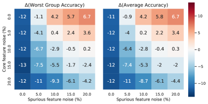
Figure 1: The improvement of last layer retraining accuracy (%) before v.s. after ERM training on Dominoes dataset (Shah et al.,, 2020). The model is initialized with ImageNet pretrained parameters. The x-axis and y-axis represent noise levels of the spurious and core features, respectively. ERM training helps/harms the performance when the non-realizable noise of core features is smaller/greater than that of the spurious features. Experiment settings are in Section 5.

Real-world datasets are riddled with features that are “right for wrong reasons” (Zhou et al.,, 2021). For instance, in Waterbirds (Sagawa et al.,, 2019), the bird type can be highly correlated with the spurious feature image backgrounds, and in CelebA (Liu et al.,, 2015) the hair color can be relevant to the gender. These features are referred to as spurious features (Hovy and Søgaard,, 2015; Blodgett et al.,, 2016; Hashimoto et al.,, 2018), being predictive for most of the training examples, but are not truly correlated with the intrinsic labeling function. Machine learning models that minimize the average loss on a training set (ERM) rely on these spurious features and will suffer high errors in environments where the spurious correlation changes. Most previous works seek to avoid learning spurious features by minimizing subpopulation group loss (Duchi et al.,, 2019), by up-weighting samples that are misclassified (Liu et al.,, 2021), by selectively mixing samples Yao et al., (2022), and so on. The general goal is to recover the core features under spurious correlations.

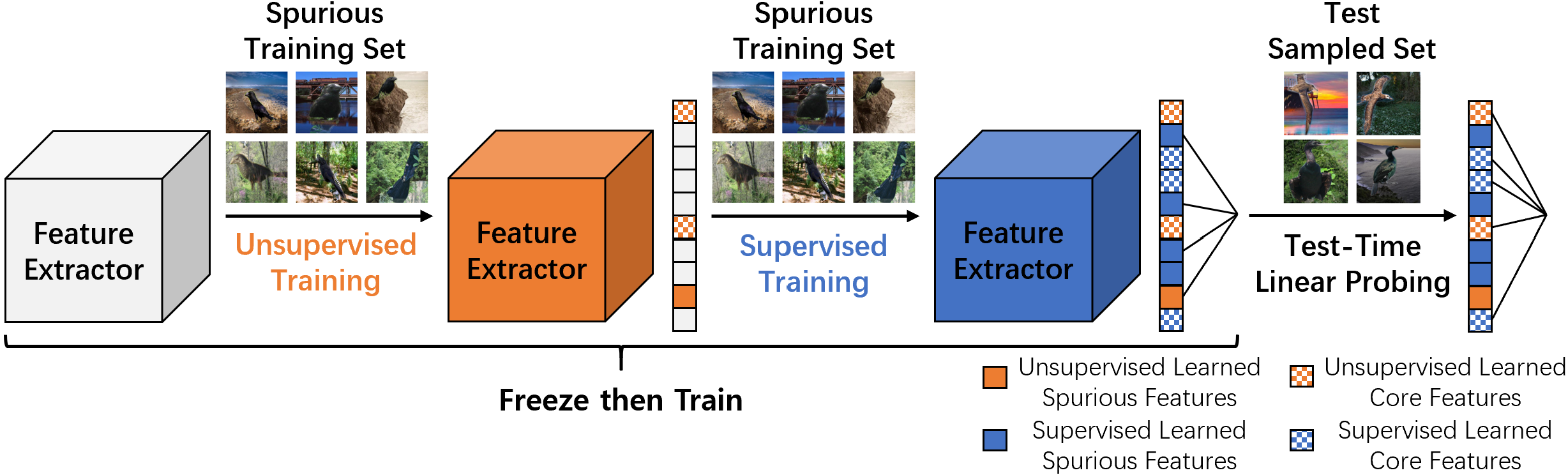
Figure 2: An illustration of our method, Freeze then Train (FTT). We start with a pretrained feature extractor (e.g. CNN) and find dataset-specific salient features using any unsupervised method like contrastive learning or PCA (the orange part). We then freeze these features and learn the rest of the features using any supervised method like ERM or a robust training algorithm (the blue part). In the test environment, the last layer is retrained. The pseudo-code can be found in Appendix A.

Recently, Kirichenko et al., (2022) empirically found that ERM can still learn the core features well even with the presence of spurious correlations. They show that by simply retraining the last layer using a small set of data with little spurious correlation, one can reweight on core features and achieves state-of-the-art performance on popular benchmark datasets. This method is called Deep Feature Reweighting (DFR), and it points to a new promising strategy to overcome spurious correlation: learn a feature extractor rather than a classifier, and then perform linear probing on the test environment data. This strategy is also used in many real-world applications in NLP, where the pipeline is to learn a large pretrained model and conduct linear probing in downstream tasks (Brown et al.,, 2020). It simply requires a CPU-based logistic regression on a few amount of samples from the deployed environment.

However, several problems regarding this strategy remain open. First, it is unclear when and why the core features can and cannot be learned during training and be recovered in test-time probing. Moreover, in the setting where the DFR strategy does not work well, is there an alternative strategy to learn the core features and make the test-time probing strategy work again?

In this paper, we first present a theoretical framework to quantify this phenomenon in a two-layer linear network and give both upper and lower control of the probing accuracy in Theorems 1 and 2. Our theories analyze the effect of training and retraining, which is highly nontrivial due to the non-convex nature of the problem. Our theories point out an essential factor of this strategy: the feature-dependent non-realizable noise (abbreviated as non-realizable noise). Noise is common and inevitable in real-world (Frénay and Verleysen,, 2013). For example, labels can have intrinsic variance and are imperfect, and human experts may also assign incorrect labels; in addition, noise is often heterogeneous and feature-dependent Zhang et al., (2021), and spurious features can be better correlated with labels in the training environment (Yan et al.,, 2014; Veit et al.,, 2017).

Our theories show that in order to learn core features, ERM requires the non-realizable noise of core features to be much smaller than that of spurious features. As illustrated in Figure 1, when this condition is violated, the features learned by ERM perform even worse than the pretrained features. The intuition is that models typically learn a mixture of different features, where the proportion depends on the trade-off between information and noise: features with larger noise are used less. During the last-layer probing, when the proportion of the core feature is small, we suffer more to amplify this feature. Our theories and experiments suggest that the scenario in Kirichenko et al., (2022) is incomplete, and the strategy can sometimes be ineffective.

Inspired by this understanding, we propose an algorithm, called Freeze then Train (FTT), which first learns salient features in an unsupervised way and freezes them, and then trains the rest of the features via supervised learning. We illustrate it in Figure 2. Based on our finding that linear probing fails when the non-realizable noise of spurious features is smaller (since labels incentivize ERM to focus more on features with smaller noise), we propose to learn features both with and without the guidance of labels. This exploits the information provided in labels, while still preserving useful features that might not be learned in supervised training. We show in Theorem 3 that FTT attains near-optimal performance in our theoretical framework, providing initial proof of its effectiveness.

We conduct extensive experiments to show that: (1) In real-world datasets the phenomenon matches our theories well. (2) On three spurious correlation datasets, FTT outperforms other algorithms by $1.4\%,0.3\%,4.1\%$ on average, and $4.5\%,0.4\%,9\%$ at most. (3) On more general OOD tasks such as three distribution shift datasets, FTT outperforms other OOD algorithms by $1.1\%,0.8\%,2.1\%$ on average. (4) We also conduct fine-grained ablations experiments to study FTT under different unsupervised feature fractions, and a different number of learned features.

Together, we give a theoretical understanding of the probing strategy, propose FTT that is more suitable for test-time probing and outperforms existing algorithms in various benchmarks. Even under spurious correlation and non-realizable noises, by combining ERM with unsupervised methods, we can still perform well in the test environment.

Related Works on rbustness to spurious correlations. Recent works aim to develop methods that are robust to spurious correlations, including learning invariant representations (Arjovsky et al.,, 2019; Guo et al.,, 2021; Khezeli et al.,, 2021; Koyama and Yamaguchi,, 2020; Krueger et al.,, 2021; Yao et al.,, 2022), weighting/sampling (Shimodaira,, 2000; Japkowicz and Stephen,, 2002; Buda et al.,, 2018; Cui et al.,, 2019; Sagawa et al.,, 2020), and distributionally robust optimization (DRO) (Ben-Tal et al.,, 2013; Namkoong and Duchi,, 2017; Oren et al.,, 2019). Rather than learn a “one-shot model”, we take a different strategy proposed in Kirichenko et al., (2022) that conducts regression on the test environment.

Related Works on representation learning. Learning a good representation is essential for the success of deep learning models Bengio et al., (2013). The representation learning has been studied in the settings of autoencoders He et al., (2021), transfer learning Du et al., (2020); Tripuraneni et al., (2020, 2021); Deng et al., (2021); Yao et al., (2021); Yang et al., (2022), topic modeling Arora et al., (2016); Ke and Wang, (2022); Wu et al., (2022), algorithmic fairness Zemel et al., (2013); Madras et al., (2018); Burhanpurkar et al., (2021) and self-supervised learning Lee et al., (2020); Ji et al., (2021); Tian et al., (2021); Nakada et al., (2023).

2 Preliminary

Throughout the paper, we consider the classification task $\mathcal{X}\to\mathcal{Y}$, where $\mathcal{X}\subset\mathbb{R}^{d}$ and $\mathcal{Y}=[K]$. Here we use $[N]$ to denote the set $\{1,\cdots,N\}$. We denote all possible distributions over a set $E$ as $\Delta(E)$. Assume that the distribution of $({\bm{x}},y)$ is $\mathcal{E}_{tr}$ in the training environment and $\mathcal{E}_{te}$ in the test environment.

Spurious correlation. Learning under spurious correlation is a special kind of Out-Of-Distribution (OOD) learning where ${\mathbb{D}}_{tr}\not={\mathbb{D}}_{te}$. We denote the term feature as a mapping $\phi(\cdot):\mathcal{X}\mapsto{\mathbb{R}}^{m}$ that captures some property of $\mathcal{X}$. We say $\phi$ is core (robust) if $y\mid\phi(x)$ has the same distribution across $\mathcal{E}_{tr}$ and $\mathcal{E}_{te}$. Otherwise, it is spurious.

Non-realizable noise. Learning under noise has been widely explored in machine learning literature, but is barely considered when spurious correlations exist. Following Bühlmann, (2020); Arjovsky et al., (2019), we consider non-realizable noise as the randomness along a generating process (can be either on features or on labels). Specifically, in the causal path $\phi(x)_{core}\to y$, we treat the label noise on $y$ as the non-realizable noise, and call it “core noise” as it is relevant to the core features; in the causal path $y\to\phi_{spu}(x)$, we treat the feature noise on $\phi_{spu}(x)$ as the non-realizable noise, and call it “spurious noise” as it is relevant to the spurious features. As we will show, the non-realizable noise influences the model learning preference.

Goal. Our goal is to minimize the prediction error in ${\mathcal{E}_{te}}$, where spurious correlations are different from ${\mathcal{E}_{tr}}$. In this paper, we consider the new strategy proposed in Kirichenko et al., (2022) that trains a feature learner on ${\mathcal{E}_{tr}}$ and linearly probes the learned features on ${\mathcal{E}_{te}}$, which we call test-time probing (or last layer retraining). No knowledge about ${\mathcal{E}_{te}}$ is obtained during the first training stage. When deploying the model to ${\mathcal{E}_{te}}$, we are given a small test datasets $\{{\bm{x}}_{i},y_{i}\}_{i=1}^{n}$ sampled from ${\mathbb{D}}_{te}$, and we are allowed to conduct logistic/linear regression on $\phi({\bm{x}})$ and $y$ to obtain our final prediction function. The goal is that after probing on the learned features, the model can perform well in ${\mathcal{E}_{te}}$, under various possible feature noise settings.

3 Theory: Understand Learned Features under Spurious Correlation

In this section, we theoretically show why core features can still be learned by ERM in spite of spurious correlations, and why non-realizable noises are crucial. Roughly speaking, only when core noise is smaller than spurious noise, features learned by ERM can guarantee the downstream probing performance. All proofs are in Appendix D.

3.1 Problem Setup

Data generation mechanism. To capture the spurious correlations and non-realizable noises, we assume the data $\big{(}{\bm{x}},y\big{)}$ is generated from the following mechanism:

$${\bm{x}}_{1}\sim\mathbb{P}\in\Delta(\mathbb{R}^{1\times d_{1}}),y={\bm{x}}_{1}\beta+\epsilon_{core},$$

$${\bm{x}}_{2}=\begin{cases}y\gamma^{\top}+\epsilon_{spu}&{\mathcal{E}_{tr}}\\ \epsilon_{spu}&{\mathcal{E}_{te}}\end{cases}\in\mathbb{R}^{1\times d_{2}},{\bm{x}}=({\bm{x}}_{1},{\bm{x}}_{2})\in\mathbb{R}^{1\times d}.$$

Here ${\bm{x}}_{1}$ is the core feature with an invertible covariance matrix ${\bm{\Sigma}}\triangleq\mathbb{E}[x_{1}^{\top}x_{1}]$. ${\bm{x}}_{2}$ is the spurious feature that is differently distributed in ${\mathcal{E}_{tr}}$ and ${\mathcal{E}_{te}}$. $\epsilon_{core}\in\mathbb{R},\epsilon_{spu}\in\mathbb{R}^{1\times d_{2}}$ are independent core and spurious noises with mean zero and variance (covariance matrix) $\eta_{core}^{2}$ and $\eta_{spu}^{2}{\bm{I}}$ respectively. $\beta\in\mathbb{R}^{d_{1}\times 1},\gamma\in\mathbb{R}^{d_{2}\times 1}$ are normalized coefficients with unit $\ell_{2}$ norm. We assume that there exists some $k\in\mathbb{N}$ such that the top-$k$ eigenvalues are larger than the noise variance $\eta_{spu}^{2},\eta_{core}^{2}$, and $\beta$ lies in the span of top-$k$ eigenvectors of ${\bm{\Sigma}}$. This is to ensure that the signal along $\beta$ is salient enough to be learned. For technical simplicity, we also assume that all eigenvalues of ${\bm{\Sigma}}$ are distinct.

Our data generation mechanism is motivated by Arjovsky et al., (2019) (Figure 3), where we extend their data model. We allow core features to be drawn from any distribution $\mathbb{P}$ so long as ${\bm{\Sigma}}$ is invertible, while Arjovsky et al., (2019) only consider a specific form of $\mathbb{P}$. In addition, in our mechanism, labels depend on core features and spurious features depend on labels. However, our theorems and algorithms can be easily applied to another setting where both core and spurious features depend on labels. This is because the difference between the two settings can be summarized as the difference on ${\bm{\Sigma}}$, while the techniques we use do not rely on the concrete form of ${\bm{\Sigma}}$.

Models. To capture the property of features and retraining, we consider a regression task using a two-layer linear network $f({\bm{x}})={\bm{x}}{\bm{W}}{\bm{b}}$, where ${\bm{W}}\in\mathbb{R}^{d\times m}$ is the feature learner and ${\bm{b}}\in\mathbb{R}^{m\times 1}$ is the last layer that will be retrained in ${\mathcal{E}_{te}}$. We assume that the model learns a low-dimensional representation ($m\ll d$), but is able to capture the ground truth signal ($m\gg k$). Notice that the optimization over $({\bm{W}},{\bm{b}})$ is non-convex, and there is no closed-form solution. This two-layer network model has been commonly used in machine learning theory literature (Arora et al.,, 2018; Gidel et al.,, 2019; Kumar et al.,, 2022). The major technical difficulty in our setting is how to analyze the learned features and control probing performance under this non-convexity with spurious correlations. We assume the parameters are initialized according to Xavier uniform distribution.

Optimization. During the training stage, we minimize the $l_{2}$-loss $\ell_{tr}({\bm{W}},{\bm{b}})=\frac{1}{2n}\|f({\bm{X}})-{\bm{Y}}\|^{2}$ where ${\bm{X}}=({\bm{x}}_{1}^{\top},\cdots,{\bm{x}}_{n}^{\top})^{\top}$ and ${\bm{Y}}=(y_{1},\cdots,y_{n})^{\top}$. For the clarity of analysis, we consider two extremes that can help simplify the optimization while still maintaining our key intuition. First, we take an infinitely small learning rate such that the optimization process becomes a gradient flow (Gunasekar et al.,, 2017; Du et al.,, 2018). Denote the parameters ${\bm{W}},{\bm{b}}$ at training time $t$ as ${\bm{W}}(t),{\bm{b}}(t)$, and ${\bm{v}}(t)={\bm{W}}(t){\bm{b}}(t)$. Second, we consider the infinite data setting ($n\to\infty$). This is a widely used simplification to avoid the influence of sample randomness Kim et al., (2019); Ghorbani et al., (2021). The parameters are updated as

$$\partial_{t}{\bm{W}}(t) =-\nabla_{\bm{W}}\ell_{tr}({\bm{W}}(t),{\bm{b}}(t))$$

$$=-\left(\frac{{\bm{X}}^{\top}{\bm{X}}}{n}{\bm{W}}(t){\bm{b}}(t)-\frac{{\bm{X}}^{\top}{\bm{Y}}}{n}\right){\bm{b}}(t)^{\top}$$

$$=\left(\mathbb{E}[{\bm{x}}^{\top}y]-\mathbb{E}[{\bm{x}}^{\top}{\bm{x}}]{\bm{v}}(t)\right){\bm{b}}(t)^{\top}$$

$$\partial_{t}{\bm{b}}(t) =-\nabla_{\bm{b}}\ell_{tr}({\bm{W}}(t),{\bm{b}}(t))$$

$$=-{\bm{W}}(t)^{\top}\left(\frac{{\bm{X}}^{\top}{\bm{X}}}{n}{\bm{W}}(t){\bm{b}}(t)-\frac{{\bm{X}}^{\top}{\bm{Y}}}{n}\right)$$

$$={\bm{W}}(t)^{\top}\left(\mathbb{E}[{\bm{x}}^{\top}y]-\mathbb{E}[{\bm{x}}^{\top}{\bm{x}}]{\bm{v}}(t)\right).$$

In the test stage, we retrain the last layer ${\bm{b}}$ to minimize the test loss, i.e.

$$\ell_{te}({\bm{W}})=\min_{\bm{b}}\mathbb{E}_{\mathcal{E}_{te}}\frac{1}{2}\|{\bm{x}}{\bm{W}}{\bm{b}}-y\|^{2}.$$

In the test stage, the spurious correlation is broken, i.e. ${\bm{x}}_{2}=\epsilon_{spu}$. The minimum error in the test stage is $\text{err}^{*}_{te}=\eta_{core}^{2}/2$ when ${\bm{v}}=(\beta^{\top},\mathbf{0})^{\top}$.

3.2 Theoretical Analysis: Noises Matter

We are now ready to introduce our theoretical results when the core features can and cannot be learned by ERM with different levels of non-realizable noises. One important intuition on why core features can still be learned well despite the (possibly more easily learned) spurious features is that, the loss can be further reduced by using both core and spurious features simultaneously.

Lemma 1

For all ${\bm{W}}\in\mathbb{R}^{d\times m},{\bm{b}}\in\mathbb{R}^{m}$, we have

$$\ell_{tr}({\bm{W}},{\bm{b}})\geq\frac{1}{2}\mathbb{E}\|{\bm{x}}{\bm{v}}^{*}_{tr}-y\|_{2}^{2}=\frac{\eta_{core}^{2}\eta_{spu}^{2}}{2(\eta_{core}^{2}+\eta_{spu}^{2})}\triangleq{\rm err}_{tr}^{*},$$

where ${\bm{v}}^{*}_{tr}=(\alpha\beta^{\top},(1-\alpha)\gamma^{\top})^{\top}$ is the optimal coefficient for training, and $\alpha=\frac{\eta_{spu}^{2}}{\eta_{core}^{2}+\eta_{spu}^{2}}$.

Lemma 1 shows that by assigning $\alpha$ fraction of weight to the core feature $\beta$ and the rest to $\gamma$, the loss is minimized. This implies that the model will learn a mixture of both features even with large spurious correlations. More importantly, the magnitude of $\alpha$ will largely influence the probing performance. During the test stage, ${\bm{x}}_{2}$ become useless, and the trained ${\bm{W}}(t){\bm{b}}(t)$ can only recover $\alpha$ fraction of $y$, which induces a large approximation error. To this end, during the retraining the last layer coefficients should scale up in order to predict $y$ well. Meanwhile, this also scales up the weight on ${\bm{x}}_{2}$, which is merely a harmful noise, resulting in a trade-off between learning accurate core features and removing spurious features. When the core noise is small, i.e., $\alpha\approx 1$, the noise on ${\bm{x}}_{2}$ will not be scaled up much. The Waterbirds dataset considered in Kirichenko et al., (2022) has $\eta_{core}=0\%<\eta_{spu}=5\%$, falling into this region. The following theorem tells how well the ERM with last-layer probing works in this region.

Theorem 1 (Upper Bound)

Assume that ${\bm{v}}(t)$ is bounded away from $\mathbf{0}$ throughout the whole optimization, i.e. $\|{\bm{v}}(t)\|_{2}>c_{0}>0$. Then, for any $0<\eta_{core}<\eta_{spu}$, any time $t$, we have

$$\ell_{te}({\bm{W}}(t))\leq\left(1+\frac{\eta_{core}^{2}}{\eta_{spu}^{2}}\right){\rm err}^{*}_{te}+\mathcal{O}(t^{-1}).$$ (1)

Here $\text{err}_{te}^{*}={\eta_{core}^{2}}/2$ is the optimal testing error and $\mathcal{O}$ hides the dependency on $\eta_{core},\eta_{tspu},c_{0}$ and the initialized parameters. When $\frac{\eta_{core}}{\eta_{spu}}\to 0$, this theorem suggests test-time probing achieves near optimal error.

Theorem 1 gives a theoretical explanation of the last layer retraining phenomenon. It shows that the test error after retraining can be close to $\text{err}_{te}^{*}$ over time. However, this guarantee holds only when $\eta_{core}<\eta_{spu}$. The following theorem shows that when the core features have large noise, the representation learned by ERM would produce a downgraded performance after linear probing.

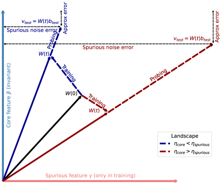
Figure 3: A toy example illustrating when and why ERM can perform well after retraining in ${\mathcal{E}_{te}}$ ($d=2,m=1$). Assume the core feature $\beta$ is vertical and the spurious feature $\gamma$ is horizontal. Both features can predict $y$ in ${\mathcal{E}_{tr}}$, while $\gamma$ is useless in ${\mathcal{E}_{te}}$ since ${\bm{x}}_{2}=\epsilon_{spu}$. We initialize our single feature ${\bm{W}}(0)$, and obtain ${\bm{W}}(t)$ after training on ${\mathcal{E}_{tr}}$. We then retrain the last layer (probing) on ${\mathcal{E}_{te}}$, i.e. rescale ${\bm{W}}(t)$ and obtain ${\bm{v}}_{test}$. When $\eta_{core}<\eta_{spu}$, ${\bm{W}}(t)$ will use $\beta$ more (the blue flow); after probing, ${\bm{v}}_{test}$ can recover $\beta$ (small approximation error) without suffering much from the spurious $\epsilon_{2}$ on the direction or $\gamma$ (small spurious noise error). On the contrary, when $\eta_{core}$ is large, ${\bm{W}}(t)$ will follow the red flow; this leads to a trade-off between two error terms. In this case, ERM performs much worse. Notice that flows in the figure are just for illustration. In practice, probing can either lengthen or shorten ${\bm{W}}(t)$, depending on the concrete form of two error terms.

Theorem 2 (Lower Bound)

Assume that in the infinity, ${\bm{W}}_{1}(\infty)\triangleq\lim_{t\to\infty}{\bm{W}}_{1}(t)$ has full column rank, which almost surely holds when $m<d$. Then for any $\eta_{core}>\eta_{spu}>0$, we have

$$\quad\lim_{t\to\infty}\frac{\ell_{te}({\bm{W}}(t))}{{\rm err}^{*}_{te}}$$

$$\geq 1+\frac{\eta_{core}^{2}}{2\eta_{spu}^{2}}\Bigg{(}1\wedge\frac{1}{2\eta_{spu}^{2}\left\|{\bm{\Sigma}}^{-1}\right\|_{2}\left\|{\bm{W}}_{1}^{\dagger}(\infty)\right\|^{2}_{2}}\Bigg{)}.$$ (2)

Here ${\bm{A}}^{\dagger}$ is the Moore-Penrose inverse of ${\bm{A}}$, and $a\wedge b$ takes the minimum over $a,b$. When $\frac{\eta_{spu}}{\eta_{core}}\to 0$, the last layer retraining error is much larger than the optimal error.

Theorem 2 implies that the error can be $\frac{\eta_{core}^{2}}{\eta_{spu}^{2}}$ times larger than $\text{err}_{te}^{*}$ when $\eta_{core}>\eta_{spu}$, showing that ERM with last layer retraining does not work in this scenario, and the features learned by ERM are insufficient to recover near-optimal performance. In summary, we prove that test-time probing performance largely relies on the non-realizable noises, and it only works when the core noise is relatively smaller. We illustrate two theorems in Figure 3.

4 Method: Improving Test-Time Probing

Our theories raise a natural question: can we improve the learned features and make the test-time probing strategy effective under various noise conditions? A feature can be better correlated with labels in ${\mathcal{E}_{tr}}$ than others, but the correlation may be spurious and even disappears in ${\mathcal{E}_{te}}$. Without concrete knowledge about ${\mathcal{E}_{te}}$ and spurious correlations, it is impossible to determine whether or not a learned feature is informative only in ${\mathcal{E}_{tr}}$, especially given that there are innumerable amount of features. This problem comes from treating the label as an absolute oracle and is unlikely to be addressed by switching to other supervised robust training methods that still depend on labels. We experimentally verify this in Section 5.2.

In order to perform well in test-time probing under different noise conditions, we should also learn salient features that are selected without relying on labels. This helps preserve features that are useful in the testing stage, but are ruled out because they are less informative than other features w.r.t. labels. By learning features both with and without the help of labels, we can extract informative features and simultaneously maximize diversity. To this end, we propose the Freeze then Train (FTT) algorithm, which first freezes certain salient features unsupervisedly and then trains the rest of the features supervisedly. The algorithm is illustrated in Figure 2, and we describe the details below.

4.1 Method: Freeze then Train

Algorithm 1 Freeze Then Train

0:  Dataset ${\mathbb{S}}=\{{\bm{x}}_{i},y_{i}\}_{i=1}^{n}$, initialized feature extractor $\mathcal{M}:\mathcal{X}\mapsto\mathbb{R}^{m}$, unsupervised fraction $p$, n_class $K$.

1:  Conduct PCA on $\{\mathcal{M}({\bm{x}}_{i})\}_{i=1}^{n}$ with dimension $pm$, obtain transform matrix ${\bm{W}}_{ul}\in\mathbb{R}^{m\times pm}$

2:  Set unsupervised model $\mathcal{M}_{ul}({\bm{x}})=\mathcal{M}({\bm{x}}){\bm{W}}_{ul}$, and freeze its parameters (including ${\bm{W}}_{ul}$)

3:  set $\mathcal{M}_{sl}({\bm{x}})=\mathcal{M}({\bm{x}}){\bm{W}}_{sl}$, initialize linear head $h:{\mathbb{R}}^{m}\mapsto\mathbb{R}^{K}$.

4:  Supervisedly train the model $\mathcal{M}_{FTT}({\bm{x}})=h((\mathcal{M}_{ul}({\bm{x}}),\mathcal{M}_{sl}({\bm{x}}))$ on ${\mathbb{S}}$ using ERM, update $\mathcal{M}_{sl},{\bm{W}}_{sl},h$ until converge.

4:  $\mathcal{M}_{FTT}$

Step 1. Unsupervised freeze stage. FTT starts with a model $\mathcal{M}_{init}$ pretrained in large datasets like ImageNet or language corpus. Given a training set ${\mathbb{S}}_{tr}\sim{\mathbb{D}}_{tr}$, we use an unsupervised method like Contrastive Learning or Principal Component Analysis (PCA) to learn $pm$ features, where $m$ is the number of total features, and $p\in[0,1]$ is a hyper-parameter denoting the fraction of unsupervised features. This stage gives a submodel $\mathcal{M}_{ul}:\mathcal{X}\mapsto\mathbb{R}^{pm}$, where $ul$ stands for “unsupervised learning”.

Step 2. Supervised train stage. Then, we freeze $\mathcal{M}_{ul}$ and train the other $(1-p)m$ dimensional features as well as a linear head together using a supervised method. Specifically, we copy the initial pretrained checkpoint $\mathcal{M}_{init}$, i.e. we set $\mathcal{M}_{sl}=\mathcal{M}_{init}$. We set its output dimension to $(1-p)m$, and add a linear head $h$ upon $(\mathcal{M}_{ul},\mathcal{M}_{sl})$ with input dimension $pm+(1-p)m=m$. In this way, the complete network output is $\mathcal{M}_{FTT}({\bm{x}})=h((\mathcal{M}_{ul}({\bm{x}}),\mathcal{M}_{sl}({\bm{x}}))$. We supervisedly train $\mathcal{M}_{FTT}$ where only the parameters in $h$ and $\mathcal{M}_{sl}$ is optimized (with $\mathcal{M}_{ul}$ being frozen).

4.2 Theoretical Guarantees of FTT

We now show that in our two-layer network setting, FTT can guarantee a better probing performance than ERM under different non-realizable noises. Suppose in the freeze stage, the representation learned by PCA is $\tilde{{\bm{W}}}_{ul}\in\mathbb{R}^{d\times pm}$. We similarly initialize ${\bm{W}}_{sl}(t)\in\mathbb{R}^{d\times(1-p)m},{\bm{b}}(t)=\begin{pmatrix}{\bm{b}}_{ul}(t)\\ {\bm{b}}_{sl}(t)\end{pmatrix}\in\mathbb{R}^{m\times 1}$, and train ${\bm{W}}_{FTT}(t)=({\bm{W}}_{ul},{\bm{W}}_{sl}(t))$ and ${\bm{b}}(t)$. Notice that ${\bm{W}}_{ul}$ will not be updated.

Theorem 3 (FTT Bound)

Suppose $p>\frac{k}{m}$. We still assume that throughout the whole optimization, $\|{\bm{W}}_{sl}(t){\bm{b}}_{sl}(t)\|_{2}>c_{0}>0$. Then, for any time $t$, any $\eta_{core}^{2}\not=-\eta_{spu}^{2}\beta\left(\eta_{spu}^{2}{\bm{I}}-{\bm{\Sigma}}\right)^{-1}{\bm{\Sigma}}\beta$ (which is true a.s.),

$$\ell_{te}({\bm{W}}_{FTT}(t))\leq{\rm err}_{te}^{*}+\mathcal{O}(t^{-1}).$$ (3)

Theorem 3 suggests that when we preserve enough unsupervised features, FTT can converge to the optimum in ${\mathcal{E}_{te}}$ for most of $\eta_{core}$ and $\eta_{spu}$. It can circumvent the lower bound in Theorem 2 where one only uses ERM ($p=0$); it can also outperform the pure unsupervised method, since pure PCA features cannot attain $\text{err}_{tr}^{*}$ either. It is by combining both features in ${\bm{W}}_{ul}$ and ${\bm{W}}_{sl}$ that FTT can surprisingly reach the optimum. This effectiveness will be further verified by thorough experiments in the next section.

4.3 Discussions on FTT

Selection of training algorithms. Notice that FTT is a meta-algorithm, since it can be built on any supervised and unsupervised method. To illustrate the effectiveness of our method, in this paper we simply use PCA in the “freeze” stage and ERM in the “train” stage. This ensures that the effectiveness of FTT does not take advantage of other algorithms that are carefully designed for these tasks.

Selection of $p$. The unsupervised fraction $p$ is the only hyper-parameter. In terms of expressiveness, FTT is strictly stronger than a supervisedly trained model with features $(1-p)m$. We verify in Section 5.3.1 that FTT works well with various selection of $p$, e.g. between $[0.25,0.75]$.

Computational cost. Although FTT is twice as large as the base model $\mathcal{M}_{init}$, in the supervised training stage the size of parameters to be optimized remains unchanged, since $\mathcal{M}_{ul}$ is frozen. In practice, we find that the computation time and the GPU memory cost are indeed unchanged in each epoch. For the “freeze” stage, we only conduct a PCA, which can be quickly done even in CPU. For more discussions, please refer to Appendix A.

5 Experiments

In this section, we experimentally verify our theories in real-world datasets, compare FTT with other algorithms, and conduct ablations. An overview of our experimental setup is provided below; see Appendix B for more details.

Noise generation. To systematically study the influence of noise, we follow Zhang et al., (2021) and explicitly generate noise by flipping labels. Notice that labels are noisy for all data we obtain, no matter what the training set ${\mathbb{S}}_{tr}\sim{\mathcal{E}_{tr}}$ and the test-time probing set ${\mathbb{S}}_{te}\sim{\mathcal{E}_{te}}$ are. Nevertheless, our goal is to recover the ground truth. To accurately evaluate the method, we further divide ${\mathbb{S}}_{te}$ into a validation split ${\mathbb{S}}_{val}$ and a testing split ${\mathbb{S}}_{te}$. The labels are noisy in ${\mathbb{S}}_{tr}$ and ${\mathbb{S}}_{val}$, but are noiseless in ${\mathbb{S}}_{te}$. We retrain the last layer using only the validation split, and report performance on the testing split that is never seen.

Datasets. We consider Waterbirds (Sagawa et al.,, 2019) and CelebA (Liu et al.,, 2015), as well as Dominoes used in Shah et al., (2020); Pagliardini et al., (2022).

• Dominoes is a synthesis dataset based on CIFAR10 and MNIST. The top half of the image shows CIFAR10 images (core features) and the bottom half shows MNIST images (spurious features). Digits are spuriously correlated to labels in ${\mathcal{E}_{tr}}$, but are independent with labels in ${\mathcal{E}_{te}}$. Given a target core noise $\eta_{core}$ and spurious noise $\eta_{spu}$, we first randomly flip $\eta_{core}$ fraction of the ground truth in CIFAR to obtain $y_{core}$ and $\eta_{spu}$ fraction of the ground truth in MNIST to obtain $y_{spu}$. For ${\mathcal{E}_{tr}}$, we concatenate CIFAR and MNIST images with the same label, i.e. $y_{core}=y_{spu}$. For ${\mathcal{E}_{te}}$, digits are randomly concatenated with CIFAR images. We select the $\eta_{core}$ and $\eta_{spu}$ separately from $\{0,5,10,15,20\}$ ($\%$), resulting in 25 settings of noise.

• Waterbirds is a typical spurious correlation benchmark. The label is the type of bird (water-bird $=0$ or ground-bird $=1$), which is spuriously correlated with the background (water $=0$ or ground $=1$). In the training split ${\mathbb{S}}_{tr}$, the spurious noise $\eta_{spu}$ is $5\%$, while in ${\mathbb{S}}_{val}$ and ${\mathbb{S}}_{te}$ we have $\eta_{spu}=50\%$. Given $\eta_{core}$, we flip the label of the dataset according to Table 1. For example, we select ${\color[rgb]{0,0,0.545}\frac{p}{2}\eta_{core}}$ fraction of data from $(0,0)$ and flip labels to $1$. This will increase $\eta_{core}$ and $\eta_{spu}$ by $\frac{p}{2}\eta_{core}$. We also select ${\color[rgb]{0.545,0,0}\frac{p}{2}\eta_{core}}$ fraction of data from $(0,1)$ and flip labels to $1$. This will increase $\eta_{core}$ but decrease $\eta_{spu}$ by $\frac{p}{2}\eta_{core}$. Similarly, we flip $\frac{1-p}{2}\eta_{core}$ fraction of data with label $1$. After flipping, the spurious noise is kept unchanged, but the core noise increases from $0$ to $\eta_{core}$. We select $\eta_{core}$ from $\{0,2,4,6,8,10\}$ in percentage. The spurious noise in the ${\mathbb{S}}_{tr},{\mathbb{S}}_{val},{\mathbb{S}}_{te}$ is $5\%,50\%,50\%$.

  (Core, Spurious)	Origin fraction	Flip fraction
  $(0,0)$	$p_{0}s$	${\color[rgb]{0,0,0.545}-\frac{p_{0}}{2}\eta_{core}}{\color[rgb]{0.545,0,0}+\frac{p_{1}}{2}\eta_{core}}$
  $(0,1)$	$p_{0}(1-s)$	${\color[rgb]{0.545,0,0}-\frac{p_{0}}{2}\eta_{core}}{\color[rgb]{0,0,0.545}+\frac{p_{1}}{2}\eta_{core}}$
  $(1,0)$	$p_{1}(1-s)$	${\color[rgb]{0,0,0.545}+\frac{p_{0}}{2}\eta_{core}}{\color[rgb]{0.545,0,0}-\frac{p_{1}}{2}\eta_{core}}$
  $(1,1)$	$p_{1}s$	${\color[rgb]{0.545,0,0}+\frac{p_{0}}{2}\eta_{core}}{\color[rgb]{0,0,0.545}-\frac{p_{1}}{2}\eta_{core}}$

  Table 1: The fraction of data to be flipped to generate core noise $\eta_{core}$ in Waterbirds and CelebA. The (Core, Spurious) column represents the label of the core feature and the spurious feature. $p_{0},p_{1}$ is the fraction of data with label $0,1$, and $s$ is the spurious correlation.

• CelebA is a binary classification dataset, where the label is the color of hair (non-blond $=0$ or blond $=1$), and is spuriously correlated with the gender (female $=0$ or male $=1$). The major difference between CelebA and Waterbirds is that the spurious noise in CelebA is large ($42\%$). To better study the probing performance under different noises, we drop a fraction of data with (color, gender) $=(0,0)$ such that $\eta_{spu}$ in ${\mathbb{S}}_{tr}$ is kept to $6\%$ within data groups with label $0$ and $1$. The label flipping process is the same as in Waterbirds.

Dataset	$\eta_{core}$ (%)	Worst Group Accuracy (%)						Average Accuracy (%)
		ERM	IRM	CVaR-DRO	JTT	Ours		ERM	IRM	CVaR-DRO	JTT	Ours
Waterbirds	0	95.0	95.3	94.3	93.3	94.5		95.3	95.5	94.6	94.1	94.9
	2	93.6	94.1	93.8	89.7	93.6		94.2	94.3	94.0	90.7	94.2
	4	92.8	92.8	92.8	85.3	92.9		93.2	93.5	93.2	85.9	93.5
	6	90.8	91.5	77.8	86.8	92.8		91.3	91.8	77.8	87.1	92.9
	8	88.5	88.8	77.8	82.0	92.7		89.9	90.1	77.8	82.7	93.0
	10	87.6	87.9	77.8	78.6	92.4		89.4	89.4	77.8	78.9	92.9
	Mean	91.4	91.7	85.7	86.0	93.1		92.2	92.4	85.9	86.6	93.6
CelebA	0	95.0	95.2	92.9	94.4	95.3		97.2	97.2	96.0	96.7	97.2
	2	95.2	95.2	92.4	91.6	95.2		97.2	97.2	95.9	96.0	97.2
	4	94.5	94.2	91.9	92.7	94.9		97.1	97.0	95.5	96.4	97.2
	6	94.3	94.3	91.5	92.0	94.4		96.9	96.9	95.5	96.0	97.0
	8	93.7	93.8	91.4	91.4	94.0		96.7	96.7	95.4	95.7	96.7
	10	92.4	92.8	91.1	80.5	93.1		96.2	96.2	95.4	92.1	96.3
	Mean	94.2	94.2	91.9	90.4	94.5		96.9	96.9	95.6	95.5	96.9

Table 2: Test-time probing accuracy (%) for four methods on Waterbirds and CelebA, under different core noises $\eta_{core}$. Bold means the best accuracy across four methods. The “Mean” row stands for the average accuracy across $\eta_{core}$. We repeat all settings $10$ times and average the numbers. For worst group accuracy, FTT (ours) can be competitive when $\eta_{core}$ is small and outperform other algorithms by at most $4.5\%$ when $\eta_{core}$ increases. It can increase accuracy by $1.4\%$ and $0.3\%$ on Waterbirds and CelebA on average.

Models. For Dominoes we use ResNet18 (He et al.,, 2016), and for Waterbirds and CelebA we use ResNet50. We load ImageNet pretrained weights (Tanaka et al.,, 2018) from torchvision.models (Paszke et al.,, 2017).

Methods. We compare FTT with ERM, IRM (Arjovsky et al.,, 2019), CVaR-DRO (Duchi et al.,, 2019) and JTT (Liu et al.,, 2021). IRM is a widely used OOD generalization algorithm, and CVaR-DRO and JTT are competitive robust training methods that perform well in several benchmark datasets for studying spurious correlations. For IRM, we use hyperparameters in We use hyperparameters in Gulrajani and Lopez-Paz, (2020). For CVaR-DRO and JTT, we use hyperparameters searched in Liu et al., (2021). For ERM and test-time probing, we use parameters in Kirichenko et al., (2022). For FTT, we set $p=0.25$.

Test-time Probing. After we train a model in ${\mathbb{S}}_{tr}$, we need to retrain the last layer in ${\mathbb{S}}_{val}$. We follow Kirichenko et al., (2022) and divide ${\mathbb{S}}_{val}$ into two subsets, where the first subset is used to retrain the last layer, and the second is to select hyperparameters. Specifically, We sub-sample the first subset using the group information such that the data population from each of the two groups are identical. We then perform logistic regression on this sub-sampled dataset. This process is repeated for 10 times, and we average these learned linear weights and obtain the final last layer weight and bias. We then use the second group to select the hyperparameters, i.e. the regularization term $C$ according to the worst spurious group accuracy. After probing, we save the model and evaluate the worst group accuracy and the average accuracy in the test split where the label is noiseless. For Dominoes, each setting is repeated for 5 times; for Waterbirds and CelebA 10 times. Each reported number is averaged across these runs.

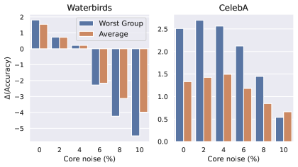
Figure 4: Test-time probing accuracy gap between trained model $\mathcal{M}_{erm}$ and initialized model $\mathcal{M}_{init}$ on Waterbirds and CelebA. The x-axis is the core noise and the y-axis is the improvement of accuracy. In both datasets, the improvement of both worst group accuracy and average accuracy decrease when $\eta_{core}$ increases. In Waterbirds, large $\eta_{core}$ can even make ERM training harmful.

5.1 Examine Non-realizable Noise Theories

Noise matters in Dominoes.

We compare the test-time probing accuracy gap between the ERM-trained model $\mathcal{M}_{erm}$ and initialized model $\mathcal{M}_{init}$ under different noises in Figure 1. When $\eta_{core}<\eta_{spu}$ (the upper-triangle part), the probing accuracy improved by $6.7\%$ (both for the worst group and in average). However, as $\eta_{core}$ increases or $\eta_{spu}$ decreases, this accuracy improvement diminishes from $6.7\%$ to $-12\%$. The trends are clear if we consider any certain row or column, where $\eta_{core}$ ($\eta_{spu}$) is fixed and $\eta_{spu}$ ($\eta_{core}$) alters. Despite ERM learns core features when $\eta_{core}<\eta_{spu}$, it cannot preserve them when $\eta_{core}>\eta_{spu}$.

Noise matters in Waterbirds and CelebA.

We now turn to Waterbirds and CelebA. We similarly save $\mathcal{M}_{erm}$ as well as $\mathcal{M}_{init}$, calculate their probing accuracies, and show the gap in Figure 4. In both datasets, test-time probing accuracy decreases when $\eta_{core}$ increases. For instance, for worst group accuracy, the improvement is $1.81\%$ for Waterbirds and $2.5\%$ for CelebA when $\eta_{core}=0$, but becomes $-5.5\%$ for Waterbirds and $0.5\%$ for CelebA when $\eta_{core}=10\%$. In Waterbirds, ERM becomes detrimental even when $\eta_{core}=6\%$ is slightly larger than $\eta_{spu}=5\%$.

5.2 Effectiveness of FTT

5.2.1 Spurious Correlation Benchmarks

We now compare FTT with other algorithms, and show results in Table 2. For the worst group accuracy, FTT attains $93.1\%$ in Waterbirds and $94.5\%$ in CelebA on average, outperforming ERM and other robust training algorithms by $1.4\%$ and $0.3\%$. When $\eta_{core}$ is small, purely supervised methods can perform quite well, and FTT can match their performance. When $\eta_{core}$ increases, purely supervised based algorithms are biased to learn more spurious features, while FTT can resist non-realizable noises during training. In waterbirds, it can recover accuracy by $4.5\%$.

An interesting observation is the performance of CVaR-DRO and JTT. They are robust training algorithms that intuitively emphasize the importance of samples that are incorrectly classified. It turns out that this focus could be misleading where there exist non-realizable noises, since the emphasized samples can be classified wrong because of the noise. In Waterbirds, they perform nearly $10\%$ worse than ERM, suggesting that relying too much on labels might backfire in situations where we do not know if features can be noisy. On the contrary, FTT overcomes this problem by finding features in an unsupervised way.

We also compare FTT with ERM in Dominoes, and show results in Appendix C. Averaged across 25 noise settings, FTT attains $78.1\%$ (worst group) and $78.8\%$ (average), outperforming ERM by $4.1\%$ and $4.0\%$. Together, FTT shows the ability under different noises, overcoming the drawback of ERM when $\eta_{core}$ is large.

5.2.2 General Distribution Shift Benchmarks

To further illustrate the effectiveness of FTT, we consider more general distribution shift benchmarks, where there is no explicit spurious correlation and explicit noise between features and labels. Specifically, we consider three OOD multi-class classification datasets: PACS with 7 classes (Li et al.,, 2017), Office-Home with 65 classes (Venkateswara et al.,, 2017), and VLCS with 5 classes (Torralba and Efros,, 2011). Each dataset has four domains, and images in different domains have different styles, e.g. sketching, painting, or photography. The task is to train a model on three domains, and perform well in the unseen test domain. Following the last layer retraining setting, we also allow the model to retrain the last linear layer on the unseen test domain, i.e. we still consider the retraining accuracy.

PACS	Domain	A	C	P	S	Mean
	ERM	89.2	93.2	95.8	88.4	91.7
	IRM	61.1	67.5	81.7	79.1	72.4
	DRO	91.9	92.7	95.8	91.3	93.0
	Ours	92.7	94.9	97.9	90.8	94.1
Office- Home	Domain	A	C	P	R	Mean
	ERM	69.9	69.9	87.8	78.8	76.6
	IRM	25.2	44.9	69.3	54.0	48.3
	DRO	72.8	73.1	88.5	79.9	78.6
	Ours	73.8	73.7	87.1	83.1	79.4
VLCS	Domain	C	L	S	V	Mean
	ERM	99.3	75.0	77.3	81.5	83.3
	IRM	75.3	62.5	59.5	60.4	64.4
	DRO	99.6	74.0	78.5	81.8	83.5
	Ours	100.0	76.6	81.1	84.6	85.6

Table 3: Test-time probing accuracy (%) for 4 methods on PACS, Office-Home, and VLCS. Rows “Domain” specify which domain among 4 domains is unseen during the training stage, therefore used to retrain the last layer. The “Mean” column stands for the average accuracy across different test domain selections, and we bold the highest accuracy among 4 methods in each setting. FTT (ours) consistently outperforms other methods by 1.1% on PACS, 0.8% on Office-Home, and 2.1% on VLCS.

We compare FTT with ERM, IRM, as well as GroupDRO(Sagawa et al.,, 2019), and we use the implementation and hyperparameters in Gulrajani and Lopez-Paz, (2020). Specifically, for each dataset and each domain as the test domain, we use the default settings (for FTT, $p=0.25$) to train a model using each algorithm on the rest three domains, retrain the last layer on the test domain using linear regression, and report the accuracy. Notice that GroupDRO is different from CVaR-DRO where the latter does not rely on group information. We report all numbers in Table 3.

Across three datasets, 12 test domain settings, FTT consistently outperforms all other methods by 1.3% on average. Importantly, FTT is initially designed to remove spurious correlations, which is a special type of OOD generalization. However, we find that it also works well in general OOD settings such as in distribution shift datasets, showing that FTT is robust and effective.

5.3 Ablation Studies

5.3.1 Selection of p (unsupervised fraction)

$\eta_{core}$ (%)	unsupervised features fraction ($p$)
	0.00	0.25	0.5	0.75	1.00
0	95.0	94.5	94.8	94.6	93.2
2	93.6	93.6	94.3	94.1	92.9
4	92.8	92.9	93.2	93.7	92.6
6	90.8	92.8	93.3	93.3	93.0
8	88.5	92.7	92.6	93.0	92.7
10	87.6	92.4	93.1	93.0	93.1
Mean	91.4	93.1	93.6	93.6	92.9

Table 4: Worst group accuracy on Waterbirds, under different $p$. The setting is the same as table 2. For all $p\in[0.25,0.75]$, FTT outperforms ERM by at least $1.7\%$. We find that the best $p$ value increases as $\eta_{core}$ increases.

FTT is a simple but effective framework, where the only hyperparameter is the fraction of unsupervised features $p$. We now compare the worst group accuracy of FTT on Waterbirds under different $p$ values in Table 4. When $p=0$, FTT is the same as ERM; when $p=1$, FTT is the same as PCA. We find that FTT is relatively insensitive to $p$, with that no matter $p=0.25,0.5,0.75$, FTT can consistently outperform ERM by at least $1.7\%$. On the other hand, we do find that as the noise increases, a more “unsupervised” method is favored, which matches our expectation. The ablation on other datasets can be found in Appendix C.

5.3.2 Number of features

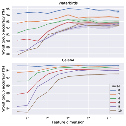
Figure 5: Worst group accuracy on Waterbirds and CelebA for FTT. The x-axis is the feature dimension in log scale.

How many features do we actually need to make last layer retraining work? This is important since in ${\mathcal{E}_{te}}$ the computation resource is limited, and preserving too many features is impractical. To this end, we use PCA to project the features that are learned in ${\mathcal{E}_{tr}}$, and then retrain the last layer on the low-dimensional features. Since PCA does not require group information (not even labels), it can be accomplished in ${\mathcal{E}_{tr}}$. We consider the projection dimension varying from $2^{1}$ to $2^{12}$, and show results in Figure 5. After training on ${\mathcal{E}_{tr}}$, only a few features are enough to perform well (or even better) in ${\mathcal{E}_{te}}$. Averaged across different noise settings, FTT attains $93.2\%$ on Waterbirds and $94.2\%$ on CelebA when $m=64$, matching $93.1\%$ and $94.5\%$ when using all features, and speeding up the probing process $3.9$ times. This suggests that FTT is computational friendly in test-time probing, and the improvement is significant.

6 Conclusions

In this paper, we study the test-time probing strategy as a way to overcome spurious correlations. We theoretically and empirically show that ERM recovers core features only when the non-realizable noise of core features is much smaller than the that of spurious features. We propose FTT to overcome this problem and outperform other algorithms under different settings. Our work suggests that by properly combining unsupervised and supervised methods, machine learning models can be more robust and accurate to spurious correlations.

Appendix A More Discussion on FTT

In practice, for the unsupervised learning, we conduct PCA using sklearn.decomposition.PCA. When the population of ${\mathbb{S}}_{tr}$ is too large, we can randomly sub-sample the dataset before PCA, which does not influence the quality of the learned features. Notice that when the initialized model $\mathcal{M}$ is random (e.g. rather than an ImageNet pretrained model), pure PCA will not work. In this case, we can consider any unsupervised training method, like the Contrastive Learning algorithm (Zhang et al.,, 2022). However, if these unsupervised methods still fail to extract core features (such as when the core features are too complex for any unsupervised methods to learn), FTT might degrade to simple ERM.

After the unsupervised training, we reinitialize a model $\mathcal{M}_{sl}$ with $(1-p)m$ features. During the supervised training, we concatenate $pm$ unsupervised features and $(1-p)m$ supervised features, apply a linear layer on the $m$ features to obtain $K$ outputs where $K$ is the number of classes, and compute the cross entropy loss with labels. We only update parameters in the last linear layer and the supervised model (with $(1-p)m$ features), while the unsupervised model $\mathcal{M}_{ul}$ is kept unchanged. As a result, the training time remains unchanged during the supervised training, since the number of parameters to be optimized remains unchanged.

Appendix B Experimental Details

In this section, we give details on how we implement our experiments.

B.1 Benchmarks

As mentioned in the main paper, we consider Dominoes, Waterbirds and CelebA, which is the same as in Kirichenko et al., (2022). For each dataset, the core feature and the spurious feature are different. In Dominoes, the core feature is the CIFAR image (car = 0, truck = 1), and the spurious feature is the MNIST digits (zero = 0, one = 1). In Waterbirds, the core feature is the type of bird (water-bird = 0, ground-bird = 1), and the spurious feature is the background (water = 0, ground = 1). In CelebA, the core feature is the color of the hair of the person in the image (Non-blond = 0, Blond = 1), while the spurious feature is the gender of the person (Female = 0, Male = 1).

The number of data we use for each split is shown in Table 5. Notice that this table shows the dataset when no noise is explicitly added. In Dominoes, the spurious correlation is perfect in ${\mathbb{S}}_{tr}$ but is complete broken in ${\mathbb{S}}_{val}$ and ${\mathbb{S}}_{te}$. Tn Waterbirds the spurious correlation in ${\mathbb{S}}_{tr}$ is 95% ($\eta_{spu}=5\%$), while in ${\mathbb{S}}_{val},{\mathbb{S}}_{te}$ it is random. In CelebA the situation is different. The spurious correlation is almost maintained in ${\mathbb{S}}_{val}$ and ${\mathbb{S}}_{te}$ (only slightly different in decimal point). This suggests that in terms of average accuracy in ${\mathbb{S}}_{te}$, pure ERM should be able to work quite well, which is verified in table 2. Notice that the original population for $(0,0)$ in ${\mathbb{S}}_{tr}$ is $71629$, and we drop most of them to create a small spurious noise for our study. Specifically, we calculate the spurious correlation within data with label $1$, which is $94.3\%$. We then select data from group $(0,0)$ sequentially until we get $x$ data such that $x/(x+66874)=94.3\%$.

(Core, Spurious)	Dominoes			Waterbirds			CelebA
	${\mathbb{S}}_{tr}$	${\mathbb{S}}_{val}$	${\mathbb{S}}_{te}$	${\mathbb{S}}_{tr}$	${\mathbb{S}}_{val}$	${\mathbb{S}}_{te}$	${\mathbb{S}}_{tr}$	${\mathbb{S}}_{val}$	${\mathbb{S}}_{te}$
(0, 0)	5000 (50)	2500 (25)	500 (25)	3498 (73)	467 (39)	2255 (39)	4053 (4)	524 (4)	546 (2)
(0, 1)	0 (0)	2500 (25)	500 (25)	184 (4)	466 (39)	2255 (39)	66874 (70)	8276 (70)	7535 (2)
(1, 0)	0 (0)	2500 (25)	500 (25)	56 (1)	133 (11)	642 (11)	22880 (24)	2874 (24)	2480 (23)
(1, 1)	5000 (50)	2500 (25)	500 (25)	1057 (22)	133 (11)	642 (11)	1387 (2)	182 (2)	180 (2)

Table 5: The number of data for each (core feature, spurious feature) group in Dominoes, Waterbirds and CelebA. Each cell shows the population and (the proportion in percentage).

B.2 Noise Generation

We now explain how we generate feature noise in detail. Dominoes is a synthesis dataset where we can manipulate the label and concatenate features. While in Waterbirds and CelebA this is impossible. Therefore, their noise generation mechanism is different.

Dominoes noise generation.

Assume we are given the original CIFAR dataset ${\mathbb{S}}_{CIFAR}$ and MNIST dataset ${\mathbb{S}}_{MNIST}$, and we want to generate a spurious correlation Dominoes dataset with core noise $\eta_{core}$ and $\eta_{spu}$. To this end, we first randomly flip $\eta_{core}$ fraction of labels in ${\mathbb{S}}_{CIFAR}$ and $\eta_{spu}$ fraction of labels in ${\mathbb{S}}_{MNIST}$. Then, we randomly concatenate CIFAR and MNIST images so long as their (possibly incorrect labels) are the same.

Waterbirds and CelebA noise generation.

In these two real-world datasets, we cannot randomly concatenate features. To this end, we only tune the core noise and keep the spurious noise unchanged. When a sample from $(0,0)$ is flipped to $(1,0)$, the noise of both the core feature and spurious feature increases; on the other hand, when a sample from $(0,1)$ is flipped to $(1,1)$, the core noise increases while the spurious noise decreases. We leverage this property to maintain $\eta_{spu}$ while tuning $\eta_{core}$, as shown in table 1.

B.3 Optimization

Our experiments consist of two stages, train a model, and retrain the last layer (test-time probing). In this section, we specify the parameters in the training stage.

Dominoes.

In Dominoes we only compare ERM and FTT. We start with the pretrained ResNet-18 model and follow the training settings in Shah et al., (2020). We use SGD with weight_decay = 1e-3 and lr = 0.01 and train the model for $200$ epoch. We reduce lr to $0.002$ after 50 epoch implemented by optim.lr_scheduler.LambdaLR. The batch size is set to $256$. We use the cross entropy loss implemented by F.cross_entropy.

Waterbirds and CelebA.

For these two datasets, we follow the implementation in Kirichenko et al., (2022) for algorithm ERM and FTT, and follow the implementation in Liu et al., (2021) for JTT and CVaR DRO in order to make sure the model is trained well. For ERM and FTT, we use SGD with momentum_decay = 0.9, lr = 1e-3 to train ResNet-50 models. For waterbirds we use weight_decay = 1e-3, and for CelebA we use weight_decay = 1e-4. We train the model for 100 epochs in Waterbirds and 50 epochs in CelebA, and the batch size is set to $128$. For JTT and CVaR DRO, we use the hyperparameters in Liu et al., (2021). Both methods use momentum_decay = 0.9, weight_decay = 1.0 on Waterbirds and momentum_decay = 0.9, weight_decay = 0.1 on CelebA. For CVaR DRO on Waterbirds, the learning rate is set to 1e-4, and the alpha rate is set to 0.2; on CelebA the learning rate is 1e-5 and the alpha rate is $0.00852$. For JTT, according to their paper, an ERM model is trained for $T$ epochs first, and some data samples are up-weighted. Then, another ERM model will be trained using these data. All hyperparameters are inherited from their paper. For these two algorithms, we use the best model according to their model selection method, i.e. the accuracy of a preserved validation set.

Once the training is finished, we will obtain a learned model where the final linear layer has input dimension $m$ and output dimension $2$. This layer will be removed and the Logistic Regression will be conducted on the $m$ dimensional features, as specified below.

B.4 Test-time Probing

We follow the deep feature reweighting algorithm to retrain the last layer. Specifically, assume we are given ${\mathbb{S}}_{val}$ that is sampled from ${\mathcal{E}_{te}}$ (there is still noise). We will use this dataset to retrain the last layer. Specifically, we first down-sample a balanced dataset, i.e. the population of groups with different spurious labels are the same. We then split this down-sampled dataset into two parts. We train the last layer using the first part, and evaluate the performance on the second part. Using the evaluated accuracy, we select the hyperparameter, i.e. the inverse regularization term $C$ in LogisticRegression. Finally, we fix the value of $C$, randomly sample $10$ balanced sets from ${\mathbb{S}}_{val}$, train the weight and the bias for each set, and average across them. This will be our final last layer. We do NOT use solver = liblinear and penalty = ’l1’, since we empirically found that this cannot improve the performance much, but will slow down the retraining a lot.

Once the probing is done, we evaluate the performance on ${\mathbb{S}}_{te}$, where the label is noiseless such that the numbers can accurately reflect the performance.

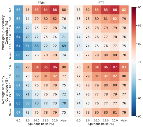
Figure 6: ERM (left) and FTT (right) worst group accuracy (top) and average accuracy (down) on Dominoes dataset, under different selection of $\eta_{core}$ and $\eta_{spu}$. The “Mean” row and column stand the average across core noise and spurious noise separately.

Appendix C Supplementary Experiments Results

FTT performs well on Dominoes.

We first show the main comparison between ERM and FTT on Dominoes in Figure 6. We find that, both methods perform well when $\eta_{core}<\eta_{spu}$. On the contrary, FTT recovers accuracy when $\eta_{core}>\eta_{spu}$ by $4\%$ in average and $9\%$ at most.

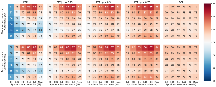
Figure 7: Worst group accuracy (top) and average accuracy (down) on Dominoes for FTT with different $p$. The first and the second column are the same as in fig. 6.

Experiments on $p$.

We next show the complete experiments on the unsupervised fraction $p$. For Waterbirds and CelebA, the results are in Table 6. We can see that both for worst group accuracy and for average accuracy, both on Waterbirds and on CelebA, FTT performs well under various selections of $p$. For Dominoes, the results are in fig. 6. Again, this plot verifies the effectiveness of FTT, and show that FTT can perform well under different selections of $p$.

Dataset	$p$	0.0	0.25	0.5	0.75	1.0		0.0	0.25	0.5	0.75	1.0
	$\eta_{core}$	Worst Group Accuracy (%)						Average Accuracy (%)
Waterbirds	0	95.0	94.5	94.8	94.6	93.2		95.3	94.9	95.2	95.0	93.7
	2	93.6	93.6	94.3	94.1	92.9		94.2	94.2	94.5	94.6	93.5
	4	92.8	92.9	93.2	93.7	92.6		93.2	93.5	93.6	94.0	93.0
	6	90.8	92.8	93.3	93.3	93.0		91.3	92.9	93.3	93.4	93.4
	8	88.5	92.7	92.6	93.0	92.7		89.9	93.0	92.9	93.3	93.1
	10	87.6	92.4	93.1	93.0	93.1		89.4	92.9	93.5	93.3	93.4
	Mean	91.4	93.1	93.6	93.6	92.9		92.2	93.6	93.8	93.9	93.4
CelebA	0	95.0	95.3	95.1	95.2	92.5		97.2	97.2	97.2	97.2	95.9
	2	95.2	95.2	95.2	94.8	92.5		97.2	97.2	97.3	97.0	95.8
	4	94.5	94.9	94.4	94.0	92.0		97.1	97.2	97.0	96.7	95.6
	6	94.3	94.4	94.1	94.1	92.2		96.9	97.0	96.9	96.8	95.7
	8	93.7	94.0	93.7	93.5	92.3		96.7	96.7	96.7	96.5	95.8
	10	92.4	93.1	92.7	93.1	91.9		96.2	96.3	96.1	96.2	95.5
	Mean	94.2	94.5	94.2	94.1	92.2		96.9	96.9	96.9	96.7	95.7

Table 6: FTT probing performance on Waterbirds and CelebA, under different unsupervised fraction $p$. This table is an extension of table 4, which only contains the worst group accuracy on Waterbirds.

Appendix D Proof of Theorems

For simplicity, for all the proofs below, we rewrite $\epsilon_{core},\epsilon_{spu}$ as $\epsilon_{1},\epsilon_{2}$, $\eta_{core},\eta_{spu}$ as $\eta_{1},\eta_{2}$, and ${\bm{W}}_{core},{\bm{W}}_{spu}$ as ${\bm{W}}_{1},{\bm{W}}_{2}$. Denote the covariance matrix of ${\bm{x}}$ as ${\bm{H}}=\mathbb{E}[{\bm{x}}^{\top}{\bm{x}}]$ (notice that ${\bm{x}}\in\mathbb{R}^{d\times 1}$). By standard algebra, we have

$${\bm{H}}=\begin{pmatrix}{\bm{\Sigma}}&{\bm{\Sigma}}\beta\gamma^{\top}\\ \gamma\beta^{\top}{\bm{\Sigma}}&\eta_{2}^{2}{\bm{I}}+(\eta_{1}^{2}+\beta^{\top}{\bm{\Sigma}}\beta)\gamma\gamma^{\top}\end{pmatrix}.$$ (4)

We denote the SVD decomposition of ${\bm{H}}=\Xi{\bm{D}}\Xi^{\top}$, where $\Xi$ is an orthogonal matrix and ${\bm{D}}$ is a diagonal matrix in descending order. We denote the SVD decomposition of ${\bm{\Sigma}}={\bm{Q}}{\bm{D}}_{1}{\bm{Q}}^{\top}$, where ${\bm{Q}}=({\bm{q}}_{1},\cdots,{\bm{q}}_{d_{1}})$ is an orthogonal matrix and ${\bm{D}}_{1}=\text{Diag}\left(\lambda_{1},\cdots,\lambda_{d_{1}}\right)$ is a descending diagonal matrix. We use ${\bm{A}}_{:n}$ to denote the first $n$ columns of ${\bm{A}}$, and $\text{span}({\bm{A}})$ to denote the linear space spanned by the column vectors of ${\bm{A}}$. Denote $g=\beta^{\top}{\bm{\Sigma}}\beta$ as the variance of ${\bm{x}}_{1}$ along the ground-truth direction $\beta$. Also recall that $\alpha=\frac{\eta_{2}^{2}}{\eta_{1}^{2}+\eta_{2}^{2}}$.

Notice that $\beta$ lies in the top $k$ eigenvectors spanned space, i.e. $\beta\in\text{span}({\bm{Q}}_{:k})$. Without loss of generality, we assume that $k$ is the minimum integer that satisfies this condition, i.e. we assume that ${\bm{q}}_{k}^{\top}\beta\not=0$. Otherwise, we decrease $k$ until this is true, while the condition $p>\frac{k}{m}$ still holds.

D.1 Proof of theorem 1

Proof sketch. To upper bound $\ell_{te}({\bm{W}}(t))$, we demonstrate that by a proper selection of ${\bm{b}}$, we have $\ell_{te}({\bm{W}}(t))\leq\frac{1}{(1-\gamma^{\top}{\bm{W}}_{2}(t){\bm{b}}(t))^{2}}\ell_{tr}({\bm{W}}(t),{\bm{b}}(t))$ (Lemma 2). Since $\eta_{core}<\eta_{spu}$, we can prove that the weight assigned on ${\bm{x}}_{2}$ is upper bounded, which help control the magnitude of $\gamma^{\top}{\bm{W}}_{2}(t){\bm{b}}(t)$. On the other hand, we follow the idea from Ali et al., (2019) to control $\ell_{tr}({\bm{W}}(t),{\bm{b}}(t))$ using some differential equation techniques (Lemma 3). This helps circumvent the direct analysis on the not-close form solution.

To upper bound test error, we first connect it with training error using the following lemma.

Lemma 2

For all ${\bm{W}},{\bm{b}}$, we have

$$\ell_{te}({\bm{W}})\leq\frac{1}{(1-\gamma^{\top}{\bm{W}}_{2}{\bm{b}})^{2}}\ell_{tr}({\bm{W}},{\bm{b}}).$$ (5)

Lemma 2 decomposes $\ell_{te}({\bm{W}}(t))$ into a factor and the training error. For simplicity, we denote $c_{t}=\gamma^{\top}{\bm{W}}_{2}(t){\bm{b}}(t)$. Below we separately bound both terms.

Bound $\ell_{tr}(t)$.

Ali et al., (2019) has pointed out that continuous time linear regression (i.e. one layer network) gives an analytical solution ${\bm{v}}(t)$. For a two layer model this remains unknown. However, since this optimization problem is convex in terms of ${\bm{v}}$ (but not of $({\bm{W}},{\bm{b}})$), in the infinity $\ell_{tr}(t)$ we can still bound the training error, which is specified by the following lemma.

Lemma 3

Under the assumption in Theorem 1, for all time step $t$, the training error is bounded by

$$\ell_{tr}({\bm{W}}(t),{\bm{b}}(t))\leq{\rm err}_{tr}^{*}+\mathcal{O}\left(\frac{1}{t}\right).$$

Bound $c_{t}$.

Notice that by standard decomposition, we have

$$\ell_{tr}({\bm{W}}(t),{\bm{b}}(t))\geq\frac{1}{2}\left((1-c_{t})^{2}\eta_{1}^{2}+\eta_{2}^{2}\|{\bm{v}}_{2}(t)\|^{2}_{2}\right)\geq\frac{1}{2}\left((1-c_{t})^{2}\eta_{1}^{2}+\eta_{2}^{2}c_{t}^{2}\right).$$

Therefore, for all time step $t$, we have

$$\frac{\eta_{1}^{2}-\sqrt{2\ell_{tr}(\eta_{1}^{2}+\eta_{2}^{2})-\eta_{1}^{2}\eta_{2}^{2}}}{\eta_{1}^{2}+\eta_{2}^{2}}\leq c\leq\frac{\eta_{1}^{2}+\sqrt{2\ell_{tr}(\eta_{1}^{2}+\eta_{2}^{2})-\eta_{1}^{2}\eta_{2}^{2}}}{\eta_{1}^{2}+\eta_{2}^{2}}.$$

Together, we have

$$\ell_{te}({\bm{W}}(t)) \leq\frac{1}{(1-c_{t})^{2}}\ell_{tr}({\bm{W}}(t),{\bm{b}}(t))$$

$$\leq\frac{1}{(1-c_{t})^{2}}\left(\mathcal{O}(\frac{1}{4t})+\text{err}_{tr}^{*}\right)$$

$$\leq\left(\frac{\eta_{1}^{2}+\eta_{2}^{2}}{\eta_{2}^{2}-\sqrt{2\ell_{tr}({\bm{W}}(t),{\bm{b}}(t))(\eta_{1}^{2}+\eta_{2}^{2})-\eta_{1}^{2}\eta_{2}^{2}}}\right)^{2}\left(\mathcal{O}(\frac{1}{4t})+\text{err}_{tr}^{*}\right)$$

$$\leq\left(\frac{\eta_{1}^{2}+\eta_{2}^{2}}{\eta_{2}^{2}-\mathcal{O}(t^{-1/2})}\right)^{2}\text{err}_{tr}^{*}+\mathcal{O}(t^{-1})$$

$$=\left(1+\frac{\eta_{1}^{2}}{\eta_{2}^{2}}\right)\text{err}^{*}_{te}+\mathcal{O}(t^{-1}).$$

D.2 Proof of Theorem 2

Proof sketch of Theorem 2. To prove the theorem, we first analyze the optimal selection of ${\bm{b}}$ given a feature matrix ${\bm{W}}$. We then convert the test error to a expression that depends on the norm of ${\bm{W}}$ in the infinity (Lemma 4). We then leverage the fact that

$$\partial_{t}\left({\bm{W}}(t)^{\top}{\bm{W}}(t)-{\bm{b}}(t){\bm{b}}(t)^{\top}\right)=\mathbf{0}$$

to connect the parameters across different $t$, and control the matrix norm using the properties of initialization (Lemma 5).

We already know that $\lim_{t\to\infty}{\bm{W}}(t){\bm{b}}(t)={\bm{W}}(\infty){\bm{b}}(\infty)={\bm{v}}^{*}$. Since ${\bm{W}}(\infty)$ has full column rank, exists $T_{0}$ such that for all $t>T_{0}$, ${\bm{W}}(t)$ has full rank and the $m^{th}$ singular value is simultaneously lower bounded by a positive constant $\lambda_{0}$ that depends only on ${\bm{W}}(\infty)$.

For any fix ${\bm{W}}$, and the test error for a given ${\bm{b}}$ is

$$\mathbb{E}_{{\bm{x}}_{2}=\epsilon_{2}}\frac{1}{2}\|{\bm{x}}{\bm{W}}{\bm{b}}-y\|^{2} =\frac{1}{2}\left(\mathbb{E}[{\bm{x}}_{1}{\bm{W}}_{1}{\bm{b}}-y]^{2}+\mathbb{E}[{\bm{x}}_{2}{\bm{W}}_{2}{\bm{b}}]^{2}+\mathbb{E}[{\bm{x}}_{1}{\bm{W}}_{1}{\bm{b}}\cdot{\bm{x}}_{2}{\bm{W}}_{2}{\bm{b}}]\right)$$ (6)

$$=\frac{1}{2}\left(\eta_{1}^{2}+\mathbb{E}\|{\bm{W}}_{1}{\bm{b}}-\beta\|_{\bm{\Sigma}}^{2}+\eta_{2}^{2}\|{\bm{W}}_{2}{\bm{b}}\|^{2}_{2}\right).$$ (7)

Since Equation 6 is convex w.r.t. ${\bm{b}}$, it is minimized when

$$\mathbf{0}=\nabla_{\bm{b}}\mathbb{E}_{{\bm{x}}_{2}=\epsilon_{2}}\frac{1}{2}\|{\bm{x}}{\bm{W}}{\bm{b}}-y\|^{2}=\left({\bm{W}}_{1}^{\top}{\bm{\Sigma}}{\bm{W}}_{1}+\eta_{2}^{2}{\bm{W}}_{2}^{\top}{\bm{W}}_{2}\right){\bm{b}}-{\bm{W}}_{1}^{\top}{\bm{\Sigma}}\beta$$ (8)

The quadratic form will not degenerate so long as $t>T_{0}$ and ${\bm{W}}_{1}(t)^{\top}{\bm{\Sigma}}{\bm{W}}_{1}(t)$ is positive definite. Together, the test error is minimized in time $t$ by setting

$${\bm{b}}_{\min}(t)=\left({\bm{W}}_{1}^{\top}(t){\bm{\Sigma}}{\bm{W}}_{1}(t)+\eta_{2}^{2}{\bm{W}}_{2}^{\top}(t){\bm{W}}_{2}(t)\right)^{-1}{\bm{W}}_{1}^{\top}(t){\bm{\Sigma}}\beta.$$

For all $t>T_{0}$, ${\bm{b}}_{\min}(t)$ is continuous in terms of $t$, i.e.

$${\bm{b}}_{\min}(t)\to{\bm{b}}_{\min}(\infty)=\left({\bm{W}}_{1}^{\top}(\infty){\bm{\Sigma}}{\bm{W}}_{1}(\infty)+\eta_{2}^{2}{\bm{W}}_{2}^{\top}(\infty){\bm{W}}_{2}(\infty)\right)^{-1}{\bm{W}}_{1}^{\top}(\infty){\bm{\Sigma}}\beta.$$

Therefore, $\lim_{t\to\infty}\ell_{te}({\bm{W}}(t))=\ell_{te}({\bm{W}}(\infty))$, and the latter is minimized by setting ${\bm{b}}$ to ${\bm{b}}_{\min}(\infty)$. For simplicity, we abbreviate ${\bm{W}}_{1}(\infty),{\bm{W}}_{2}(\infty)$ as ${\bm{W}}_{1},{\bm{W}}_{2}$. Lemma 4 below helps simplify the infinite error term, and Lemma 5 helps bound the simplified error.

Lemma 4

Under the condition in Theorem 2, we have

$$\frac{\ell_{te}({\bm{W}})}{\text{err}^{*}_{te}}=1+\frac{\eta_{1}^{2}}{\eta_{2}^{2}}\gamma^{\top}\left({\bm{I}}+\eta_{2}^{2}{\bm{W}}_{2}\left[{\bm{W}}_{1}^{\top}{\bm{\Sigma}}{\bm{W}}_{1}\right]^{-1}{\bm{W}}_{2}^{\top}\right)^{-1}\gamma$$ (9)

Lemma 5

Under the Xavier uniform initialization,

$$\lambda_{\max}^{-1}\left({\bm{I}}+\eta_{2}^{2}{\bm{W}}_{2}\left[{\bm{W}}_{1}^{\top}{\bm{\Sigma}}{\bm{W}}_{1}\right]^{-1}{\bm{W}}_{2}^{\top}\right)\geq\frac{1}{2}\wedge\frac{1}{4\eta_{2}^{2}\|{\bm{\Sigma}}\|_{2}\|{\bm{W}}_{1}^{+}\|^{2}_{2}}.$$ (10)

Combining Lemmas 4 and 5, we have

$$\lim_{t\infty}\frac{\ell_{te}({\bm{W}}(t)}{\text{err}^{*}_{te}} =\frac{\ell_{te}({\bm{W}}(\infty))}{\text{err}^{*}_{te}}$$

$$=1+\frac{\eta_{1}^{2}}{\eta_{2}^{2}}\gamma^{\top}\left({\bm{I}}+\eta_{2}^{2}{\bm{W}}_{2}\left[{\bm{W}}_{1}^{\top}{\bm{\Sigma}}{\bm{W}}_{1}\right]^{-1}{\bm{W}}_{2}^{\top}\right)^{-1}\gamma$$

$$\geq 1+\frac{\eta_{1}^{2}}{\eta_{2}^{2}}\lambda_{\max}^{-1}\left({\bm{I}}+\eta_{2}^{2}{\bm{W}}_{2}\left[{\bm{W}}_{1}^{\top}{\bm{\Sigma}}{\bm{W}}_{1}\right]^{-1}{\bm{W}}_{2}^{\top}\right)\|\gamma\|^{2}$$

$$\geq 1+\frac{\eta_{1}^{2}}{\eta_{2}^{2}}\left(\frac{1}{2}\wedge\frac{1}{4\eta_{2}^{2}\|{\bm{\Sigma}}\|_{2}\|{\bm{W}}_{1}^{+}(\infty)\|_{2}^{2}}\right).$$

D.3 Proof of Theorem 3

Proof sketch. The key intuition is that ${\bm{W}}_{ul}$ recovers important information about $\beta$, despite there is error in PCA that we can never full recover $\beta$. In this case, we can combine the features learned in ${\bm{W}}_{sl}$ and ${\bm{W}}_{ul}$ to obtain a asymptotically optimal approximation of $\beta$ without being disturbed by the spurious correlation $\gamma$. Specifically, we prove the following lemma.

Lemma 6

Exists $c_{1}\not=\frac{1-\alpha}{\alpha}$, such that

$$\begin{pmatrix}\beta\\ c_{1}\gamma\end{pmatrix}\in\text{span}\left(\Xi_{:k}\right).$$ (11)

Since our unsupervised training features ${\bm{W}}_{ul}$ takes the top $pm$ eigenvectors of $\Xi$, lemma 6 implies that $\left(\beta^{\top},c_{1}\gamma^{\top}\right)^{\top}$ lies in the span of ${\bm{W}}_{ul}$, i.e. $\exists\hat{\bm{b}}_{ul}\in\mathbb{R}^{pm\times 1}$, such that $\left(\beta^{\top},c_{1}\gamma^{\top}\right)^{\top}={\bm{W}}_{ul}\hat{\bm{b}}_{ul}$. On the other hand, we alredy know from the proof of theorem 1 in the infinity ${\bm{v}}(t)\to\left(\alpha\beta^{\top},(1-\alpha)\gamma^{\top}\right)^{\top}$. The following lemma, by combing these two crucial feature, bounds the test time probing error of ${\bm{W}}_{FTT}(t)$.

Lemma 7

By setting the retraining weight

$$\hat{\bm{b}}={\frac{c_{1}}{c_{1}\alpha-(1-\alpha)}}{\bm{W}}_{FTT}(t){\bm{b}}{(t)}-\frac{1-\alpha}{c_{1}\alpha-(1-\alpha)}\begin{pmatrix}\hat{\bm{b}}_{ul}\\ \mathbf{0}\end{pmatrix},$$

we have (recall that $c_{t}=\gamma^{\top}{\bm{W}}_{2}(t){\bm{b}}(t)$, while $c_{1}$ is fixed)

$$\ell_{te}({\bm{W}}_{FTT}(t))-\text{err}_{te}^{*} \leq\left({\frac{c_{1}}{c_{1}\alpha-(1-\alpha)}}\right)^{2}\mathcal{O}\left(\frac{\|{\bm{\Sigma}}\|_{2}\|{\bm{H}}^{-1}\|_{2}}{(\sqrt{c_{0}^{2}+1}-1)t}\right).$$ (12)

Here $\mathcal{O}$ hides a universal constant.

Notice that the RHS decays with rate $t^{-1}$. Together, the proof is finished.

Appendix E Proof of Lemmas

In this section we prove all lemmas.

E.1 Proof of Lemma 1

According to the decomposition of the training error, for any ${\bm{v}}={\bm{W}}{\bm{b}}$, we have

$$\ell_{tr}({\bm{W}},{\bm{b}}) =\frac{1}{2}\left(\mathbb{E}\|{\bm{x}}_{1}{\bm{v}}_{1}-(1-\gamma^{\top}{\bm{v}}_{2})y\|^{2}+\eta_{2}^{2}\|{\bm{v}}_{2}\|^{2}\right)$$

$$=\frac{1}{2}\left(\mathbb{E}\|{\bm{x}}_{1}{\bm{v}}_{1}-(1-\gamma^{\top}{\bm{v}}_{2}){\bm{x}}_{1}\beta\|^{2}+\eta_{1}^{2}(1-\gamma^{\top}{\bm{v}}_{2})^{2}+\eta_{2}^{2}\|{\bm{v}}_{2}\|^{2}\right)$$

$$\geq\frac{1}{2}\left(\eta_{1}^{2}(1-\gamma^{\top}{\bm{v}}_{2})^{2}+\eta_{2}^{2}\|{\bm{v}}_{2}\|^{2}\right)$$

Denote $x=\gamma^{\top}{\bm{v}}_{2}$, we have

$$\ell_{tr}({\bm{W}},{\bm{b}})\geq\frac{1}{2}\left(\eta_{1}^{2}(1-x)^{2}+\eta_{2}^{2}x^{2}\right)\geq\frac{1}{2}\cdot\frac{\eta_{1}^{2}\eta_{2}^{2}}{\eta_{1}^{2}+\eta_{2}^{2}}.$$

Here the last inequality comes from Cauchy–Schwarz inequality. The proof is finished by verifying that ${\bm{v}}^{*}_{tr}$ can indeed give the minimum.

E.2 Proof of Lemma 2

Given ${\bm{W}},{\bm{b}}$, we can decompose the training error as (denote ${\bm{v}}={\bm{W}}{\bm{b}}$)

$$\ell_{tr}({\bm{W}},{\bm{b}}) =\frac{1}{2}\mathbb{E}\|{\bm{x}}_{1}{\bm{v}}_{1}+(y\gamma^{\top}+\epsilon_{2}){\bm{v}}_{2}-y\|_{2}^{2}$$

$$=\frac{1}{2}\left(\mathbb{E}\|{\bm{x}}_{1}{\bm{v}}_{1}-(1-\gamma^{\top}{\bm{v}}_{2})y\|^{2}+\eta_{2}^{2}\|{\bm{v}}_{2}\|^{2}\right)$$

On the other hand, by setting $\hat{\bm{b}}=\frac{1}{1-\gamma^{\top}{\bm{v}}_{2}}{\bm{b}}$, the test error is upper bounded by

$$\ell_{te}({\bm{W}}) \leq\frac{1}{2}\mathbb{E}_{{\bm{x}}_{2}=\epsilon_{2}}\|{\bm{x}}{\bm{W}}\hat{\bm{b}}-y\|^{2}$$

$$=\frac{1}{2}\mathbb{E}_{{\bm{x}}_{2}=\epsilon_{2}}\|\frac{{\bm{x}}{\bm{v}}}{1-\gamma^{\top}{\bm{v}}_{2}}-y\|^{2}$$

$$=\frac{1}{2}\left(\mathbb{E}\|\frac{{\bm{x}}_{1}{\bm{v}}_{1}}{1-\gamma^{\top}{\bm{v}}_{2}}-y\|^{2}+\frac{\eta_{2}^{2}}{(1-\gamma^{\top}{\bm{v}}_{2})^{2}}\|{\bm{v}}_{2}\|^{2}\right)$$

Therefore, we have

$$\ell_{te}({\bm{W}})\leq\frac{1}{(1-\gamma^{\top}{\bm{W}}_{2}{\bm{b}})^{2}}\ell_{tr}({\bm{W}},{\bm{b}}).$$

E.3 Proof of Lemma 3

Denote ${\bm{M}}(t)={\bm{W}}(t)^{\top}{\bm{W}}(t)-{\bm{b}}(t){\bm{b}}(t)^{\top}$. Since our parameters are initialized according to Xaiver uniform distribution,

$$\|{\bm{M}}(0)\|_{2}\leq\|{\bm{W}}(0)\|^{2}_{2}+\|{\bm{b}}(0)\|_{2}^{2}\leq d\|{\bm{W}}(0)\|_{\infty}^{2}+1\leq 2.$$

Recall that ${\bm{M}}(t)$ is invariant throughout the whole optimization. We have

$$2\|{\bm{b}}(t)\|_{2}^{2}\geq{\bm{b}}(t)^{\top}{\bm{M}}(0){\bm{b}}(t)={\bm{b}}(t)^{\top}{\bm{M}}(t){\bm{b}}(t)=\|{\bm{v}}(t)\|_{2}^{2}-\|{\bm{b}}(t)\|^{4},$$

which implies that $\|{\bm{b}}(t)\|_{2}^{2}\geq\sqrt{c_{0}^{2}+1}-1$.

Convergence of ${\bm{v}}(t)$.

The gradient of ${\bm{v}}(t)$ is

$$\partial{\bm{v}}(t) =\partial_{t}{\bm{W}}(t)\cdot{\bm{b}}(t)+{\bm{W}}(t)\cdot\partial_{t}{\bm{b}}(t)$$

$$=\left({\bm{W}}(t){\bm{W}}(t)^{\top}+\|{\bm{b}}(t)\|_{2}^{2}{\bm{I}}\right)\left(\mathbb{E}[{\bm{x}}^{\top}y]-{\bm{H}}{\bm{v}}(t)\right)$$

$$=\left({\bm{W}}(t){\bm{W}}(t)^{\top}+\|{\bm{b}}(t)\|_{2}^{2}{\bm{I}}\right){\bm{H}}\left({\bm{v}}_{tr}^{*}-{\bm{v}}(t)\right)$$

where the last equation uses the fact that ${\bm{H}}$ is invertible (since ${\bm{\Sigma}}$ is invertible) and ${\bm{v}}_{tr}^{*}={\bm{H}}^{-1}\mathbb{E}[{\bm{x}}^{\top}y]$. By a standard differential equation analysis, we have

$${\bm{v}}(t)-{\bm{v}}_{tr}^{*}=\exp\left\{-{\bm{H}}\int_{0}^{t}{\bm{A}}(\tau)\mathrm{d}\tau\right\}({\bm{v}}(0)-{\bm{v}}_{tr}^{*}),$$ (13)

where ${\bm{A}}(t)\triangleq{\bm{W}}(t){\bm{W}}(t)^{\top}+\|{\bm{b}}(t)\|_{2}^{2}{\bm{I}}$ and ${\bm{A}}(t)-(\sqrt{c_{0}^{2}+1}-1){\bm{I}}$ is positive definite because the bound of $\|{\bm{b}}(t)\|^{2}_{2}$. This help us control the training error as

$$2\ell_{tr}({\bm{W}}(t),{\bm{b}}(t)) =\mathbb{E}\|{\bm{x}}{\bm{v}}(t)-y\|_{2}^{2}$$

$$={\bm{v}}(t)^{\top}{\bm{H}}{\bm{v}}(t)-2{\bm{v}}(t)^{\top}\mathbb{E}[{\bm{x}}^{\top}y]+\mathbb{E}[y^{\top}y]$$

$$={\bm{v}}(t)^{\top}{\bm{H}}{\bm{v}}(t)-2{\bm{v}}(t)^{\top}{\bm{H}}{\bm{v}}_{tr}^{*}+{\bm{v}}_{tr}^{*\top}{\bm{H}}{\bm{v}}_{tr}^{*}$$

$$\quad+\left({\bm{v}}_{tr}^{*\top}{\bm{H}}{\bm{v}}_{tr}^{*}-2{\bm{v}}_{tr}^{*\top}{\bm{H}}\mathbb{E}[{\bm{x}}^{\top}y]+\mathbb{E}[y^{\top}y\right)$$

$$=\|{\bm{v}}(t)-{\bm{v}}_{tr}^{*}\|_{{\bm{H}}}^{2}+\mathbb{E}\|{\bm{x}}{\bm{v}}_{tr}^{*}-y\|_{2}^{2}$$

$$=\|{\bm{v}}(t)-{\bm{v}}_{tr}^{*}\|_{{\bm{H}}}^{2}+2\text{err}_{tr}^{*}.$$

Plugging Equation 13 into the first term, we have

$$\|{\bm{v}}(t)-{\bm{v}}_{tr}^{*}\|_{{\bm{H}}}^{2} =({\bm{v}}(0)-{\bm{v}}_{tr}^{*})^{\top}\left[\exp\left\{-2{\bm{H}}\int_{0}^{t}{\bm{A}}(\tau)\mathrm{d}\tau\right\}{\bm{H}}\right]({\bm{v}}(0)-{\bm{v}}_{tr}^{*})$$

$$\leq\mathcal{O}\left(\left\|\exp\left\{-2{\bm{H}}\int_{0}^{t}{\bm{A}}(\tau)\mathrm{d}\tau\right\}{\bm{H}}\right\|_{2}\right)$$

$$\leq\mathcal{O}\left(\left\|\exp\left\{-2(\sqrt{c_{0}^{2}+1}-1)t{\bm{H}}\mathrm{d}\tau\right\}{\bm{H}}\right\|_{2}\right)$$

$$\leq\mathcal{O}\left(\frac{1}{(\sqrt{c_{0}^{2}+1}-1)t}\right).$$

Here the first equation is because ${\bm{H}}$ and $\int_{0}^{t}{\bm{A}}(\tau)$ are both positive definite, and can be diagonalized simultaneously. The first inequality is because $\|{\bm{v}}(0)-{\bm{v}}_{tr}^{*}\|$ is bounded, while the second is because ${\bm{A}}(t)-(\sqrt{c_{0}^{2}+1}-1){\bm{I}}$ is positive definite for all $t$.

E.4 Proof of Lemma 4

Plug in ${\bm{b}}={\bm{b}}_{\min}(\infty)$ into Equation 6, we obtain (denote ${\bm{\Lambda}}={\bm{W}}_{1}^{\top}{\bm{\Sigma}}{\bm{W}}_{1}$)

$$\ell_{te}({\bm{W}}_{1})-\text{err}^{*}_{te} =\frac{1}{2}\left({\bm{b}}^{\top}\left[{\bm{\Lambda}}+\eta_{2}^{2}{\bm{W}}_{2}^{\top}{\bm{W}}_{2}\right]^{-1}{\bm{b}}-2\beta^{\top}{\bm{\Sigma}}{\bm{W}}_{1}{\bm{b}}+\beta^{\top}{\bm{\Sigma}}\beta\right)$$

$$=\frac{1}{2}\left(\beta^{\top}{\bm{\Sigma}}\beta-\beta^{\top}{\bm{\Sigma}}{\bm{W}}_{1}\left[{\bm{\Lambda}}+\eta_{2}^{2}{\bm{W}}_{2}^{\top}{\bm{W}}_{2}\right]^{-1}{\bm{W}}_{1}^{\top}{\bm{\Sigma}}\beta\right)$$

$$=\frac{1}{2}\left(\beta^{\top}{\bm{\Sigma}}\beta-\beta^{\top}{\bm{\Sigma}}{\bm{W}}_{1}\left[{\bm{\Lambda}}^{-1}-\eta_{2}^{2}{\bm{\Lambda}}^{-1}{\bm{W}}_{2}\left({\bm{I}}+\eta_{2}^{2}{\bm{W}}{\bm{\Lambda}}^{-1}{\bm{W}}_{2}^{\top}\right)^{-1}{\bm{W}}_{2}{\bm{\Lambda}}^{-1}\right]{\bm{W}}_{1}^{\top}{\bm{\Sigma}}\beta\right)$$

where the last equation is because for any invertible ${\bm{A}},{\bm{B}}$,

$$\left({\bm{A}}+{\bm{C}}{\bm{B}}{\bm{C}}^{\top}\right)^{-1}={\bm{A}}^{-1}-{\bm{A}}^{-1}{\bm{C}}\left({\bm{B}}^{-1}+{\bm{C}}^{\top}{\bm{A}}^{-1}{\bm{C}}\right)^{-1}{\bm{C}}^{\top}{\bm{A}}^{-1}.$$

Notice that we have ${\bm{W}}_{1}{\bm{b}}(\infty)=\alpha\beta,{\bm{W}}_{2}{\bm{b}}(\infty)=(1-\alpha)\gamma$. Multiplying ${\bm{W}}_{1}^{\top}{\bm{\Sigma}}$ on both side, we have

$${\bm{\Lambda}}{\bm{b}}(\infty) =\alpha{\bm{W}}_{1}^{\top}{\bm{\Sigma}}\beta$$

$${\bm{b}}(\infty) =\alpha{\bm{\Lambda}}^{-1}{\bm{W}}_{1}^{\top}{\bm{\Sigma}}\beta.$$

This implies that

$$\beta^{\top}{\bm{\Sigma}}{\bm{W}}_{1}{\bm{\Lambda}}^{-1}{\bm{W}}_{1}^{\top}{\bm{\Sigma}}\beta =\frac{1}{\alpha}\beta^{\top}{\bm{\Sigma}}{\bm{W}}_{1}{\bm{b}}(\infty)=\beta^{\top}{\bm{\Sigma}}\beta,$$

$${\bm{W}}_{2}{\bm{\Lambda}}^{-1}{\bm{W}}_{1}^{\top}{\bm{\Sigma}}\beta =\frac{1}{\alpha}{\bm{W}}_{2}{\bm{b}}(\infty)=\frac{1-\alpha}{\alpha}\gamma.$$

Therefore, we have

$$\ell_{te}({\bm{W}}_{1})-\text{err}^{*}_{te} =\frac{(1-\alpha)^{2}}{2\eta_{2}^{2}\alpha^{2}}\left(\gamma^{\top}\left[{\bm{I}}+\eta_{2}^{2}{\bm{W}}{\bm{\Lambda}}^{-1}{\bm{W}}_{2}^{\top}\right]^{-1}\gamma\right)$$

$$=\frac{\eta_{1}^{4}}{2\eta_{2}^{2}}\gamma^{\top}\left[{\bm{I}}+\eta_{2}^{2}{\bm{W}}{\bm{\Lambda}}^{-1}{\bm{W}}_{2}^{\top}\right]^{-1}\gamma.$$

E.5 Proof of Lemma 5

We first upper bound $\|{\bm{W}}_{2}\|_{2}$. Recall an important property of our two layer linear model from Kumar et al., (2022):

$$\partial_{t}\left[{\bm{W}}(t)^{\top}{\bm{W}}(t)^{\top}-{\bm{b}}(t){\bm{b}}(t)^{\top}\right]=\mathbf{0}.$$ (14)

Applying this property with $t=0$ and $t\to\infty$, we have

$${\bm{W}}_{1}^{\top}{\bm{W}}_{1}+{\bm{W}}_{2}^{\top}{\bm{W}}_{2}-{\bm{b}}(\infty){\bm{b}}(\infty)^{\top}={\bm{W}}(0)^{\top}{\bm{W}}(0)-{\bm{b}}(0){\bm{b}}(0)^{\top}.$$

By multiplying ${\bm{W}}_{2}$ on the left and ${\bm{W}}_{2}^{\top}$ on the right,

$$\lambda_{\max}\left({\bm{W}}_{2}{\bm{W}}_{2}^{\top}{\bm{W}}_{2}{\bm{W}}_{2}^{\top}-(1-\alpha)^{2}\gamma\gamma^{\top}\right)\leq\lambda_{\max}\left({\bm{W}}_{2}{\bm{W}}(0)^{\top}{\bm{W}}(0){\bm{W}}_{2}^{\top}\right),$$

which implies that

$$\|{\bm{W}}_{2}\|_{2}^{4}-1\leq\|{\bm{W}}_{2}\|^{2}\|{\bm{W}}(0)\|_{2}^{2}.$$

Since ${\bm{W}}(0)$ is initialized according to the Xavier uniform distribution, we have

$$\|{\bm{W}}(0)\|\leq\sqrt{d}\|{\bm{W}}(0)\|_{\infty}=\sqrt{d}\cdot\frac{1}{\sqrt{d}}=1.$$

This quickly implies that $\|{\bm{W}}_{2}\|_{2}^{2}<2$.

Together, we have

$$\lambda_{\max}\left({\bm{I}}+\eta_{2}^{2}{\bm{W}}_{2}\left[{\bm{W}}_{1}^{\top}{\bm{\Sigma}}{\bm{W}}_{1}\right]^{-1}{\bm{W}}_{2}^{\top}\right) \leq 1+\eta_{2}^{2}\|{\bm{W}}_{2}\|_{2}^{2}\lambda_{\max}\left(\left[{\bm{W}}_{1}^{\top}{\bm{\Sigma}}{\bm{W}}_{1}\right]^{-1}\right)$$

$$\leq 1+2\eta_{2}^{2}\lambda_{\max}\left(\left[{\bm{W}}_{1}^{\top}{\bm{\Sigma}}{\bm{W}}_{1}\right]^{-1}\right)$$

$$\leq 1+2\eta_{2}^{2}\|{\bm{\Sigma}}^{-1}\|_{2}\|{\bm{W}}_{1}^{+}\|_{2}^{2}$$

$$\leq 2\max\left\{1,2\eta_{2}^{2}\|{\bm{\Sigma}}^{-1}\|_{2}\|{\bm{W}}_{1}^{+}\|_{2}^{2}\right\}$$

where the second last inequality comes from standard linear algebra. The proof is finished by taking the inverse.

E.6 Proof of Lemma 6

To study the span of $\Xi_{:k}$, we first need to understand the property of the eigenvector of ${\bm{H}}$. Notice that ${\bm{H}}$ is p.d. and all eigenvalue is positive. The eigenvectors of ${\bm{H}}$ can be divided into the following three groups.

1. First, consider any normalized vector $\gamma^{\perp}\in\mathbb{R}^{d_{2}\times 1}$. In this case, we have

   $${\bm{H}}\begin{pmatrix}\mathbf{0}\\ \gamma^{\perp}\end{pmatrix}=\eta_{2}^{2}\begin{pmatrix}\mathbf{0}\\ \gamma^{\perp}\end{pmatrix}.$$

   Since the space dimension of {$\gamma^{\perp}\}$ is $d_{2}-1$, we find $d_{2}-1$ eigenvector of ${\bm{H}}$ with eigenvalue $\eta_{2}^{2}$. We denote them as $(\mathbf{0}^{\top},\gamma^{\perp}_{i})^{\top},i\in[d_{2}-1]$.

2. Second, for $j>k$,

   $${\bm{H}}\begin{pmatrix}{\bm{q}}_{j}\\ \mathbf{0}\end{pmatrix}=\begin{pmatrix}{\bm{\Sigma}}{\bm{q}}_{j}\\ \beta^{\top}{\bm{\Sigma}}{\bm{q}}_{j}\end{pmatrix}=\lambda_{j}\begin{pmatrix}{\bm{q}}_{j}\\ \mathbf{0}\end{pmatrix}$$

   since $\beta$ lies in the span of the top $k$ eigenvectors of ${\bm{\Sigma}}$. This implies that for $j=k+1,\cdots,d_{1}$, $({\bm{q}}_{i}^{\top},\mathbf{0}^{\top})^{\top}$ is the eigenvector of ${\bm{H}}$ with eigenvalue $\lambda_{i}$.

3. All the eigenvector left. We denote them as ${\bm{u}}_{i}$ with eigenvector $\mu_{i}$ for $i\in[k+1]$. Notice that ${\bm{q}}_{i}(i\leq k)$ is not an eigenvector so long as $\beta^{\top}{\bm{q}}_{i}\not=0$.

The essential intuition is that for at least $k$ vectors in group 3, their eigenvalue is strictly larger than all eigenvalues in group 1 ($\eta_{2}^{2}$) and group 2 ($\lambda_{j},j>k$). To see this, denote ${\bm{u}}_{i}=({\bm{u}}_{i,1}^{\top},{\bm{u}}_{i,2}^{\top})^{\top}$. First, notice that ${\bm{u}}_{i,2}\perp\gamma^{\perp}$. Therefore, ${\bm{u}}_{i,2}$ must be in the direction of $\gamma$, i.e. ${\bm{u}}_{i,2}=r_{i}\gamma$, where $r_{i}$ can possibly be $0$. Second, ${\bm{u}}_{i,1}\perp{\bm{q}}_{j},\forall j>k$. Therefore, we can further denote ${\bm{u}}_{i,1}=\sum_{\tau=1}^{k}e_{i,\tau}{\bm{q}}_{\tau}$. In this case, since

$$\mu_{i}\begin{pmatrix}{\bm{u}}_{i,1}\\ r_{i}\gamma\end{pmatrix}={\bm{H}}{\bm{u}}=\begin{pmatrix}{\bm{\Sigma}}{\bm{u}}_{i,1}+r_{i}{\bm{\Sigma}}\beta\\ \beta^{\top}{\bm{\Sigma}}{\bm{u}}_{i,1}+r_{i}(\eta_{1}+\eta_{2}+g)\gamma\end{pmatrix},$$

which implies that for all $i\in[k+1]$,

$$e_{i,\tau}\mu_{i} =e_{i,\tau}\lambda_{\tau}+r_{i}\lambda_{\tau}b_{\tau},\forall\tau\in[k]$$ (15)

$$\mu_{i}r_{i} =\sum_{\tau=1}^{k}\lambda_{\tau}b_{\tau}(e_{i,\tau}+r_{i}b_{\tau})+r_{i}(\eta_{1}^{2}+\eta_{2}^{2}).$$ (16)

Here $\beta=\sum_{\tau=1}^{k}b_{\tau}{\bm{q}}_{\tau}$ and $b_{k}\not=0$. With this, we now specify all $k+1$ eigenvalues, start from $i=k+1$ to $i=1$. We will show that they separately fall in the interval $[0,\lambda_{k}],[\lambda_{k},\lambda_{k-1}],\cdots,[\lambda_{2},\lambda_{1}],[\lambda_{1},+\infty)$.

First, given any $i\in[k]$, When $b_{i}=0$, we can set $r_{i}=0,e_{i}=1,\mu=\lambda_{i}$ and $e_{i^{\prime}}=0,\forall i^{\prime}\not=i$. In this case, eqs. 15 and 16 are satisfied. We then find an eigenvector $({\bm{q}}_{i}^{\top},\mathbf{0}^{\top})^{\top}$ with eigenvalue $\lambda_{i}$.

On the other hand, when $b_{i}\not=0$, there must be $\mu\not=\lambda_{i}$. We set

$$e_{\tau}=\frac{r\lambda_{\tau}b_{\tau}}{\mu-\lambda_{\tau}},\forall\tau\in[k],$$

which satisfies eq. 15. Plugging into eq. 16, we have

$$\mu r=\sum_{\tau=1}^{k}\frac{r\mu\lambda_{\tau}b_{\tau}^{2}}{\mu-\lambda_{\tau}}+r(\eta_{1}^{2}+\eta_{2}^{2}),$$ (17)

which implies (denote ${\mathbb{T}}=\{i\in[k]:b_{i}\not=0\}$)

$$\mu=\sum_{\tau\in{\mathbb{T}}}\frac{\mu\lambda_{\tau}b_{\tau}^{2}}{\mu-\lambda_{\tau}}+(\eta_{1}^{2}+\eta_{2}^{2}).$$ (18)

Any positive solution $\mu$ of eq. 18 can generate an eigenvector with eigenvalue $\mu$. On the other hand, in each interval $[\lambda_{\tau},\lambda_{\tau^{\prime}}]$, the RHS decreases as $\mu$ increases, while the LHS increases as $\mu$ increases. In addition, the RHS goes to $+\infty$ when $\mu\to\lambda_{\tau}^{+}$ and goes to $-\infty$ when $\mu\to\lambda_{\tau^{\prime}}^{-}$. Therefore, there will be exactly one solution for all the intervals in $[0,+\infty)$ divided by elements in ${\mathbb{T}}$. Together, $k+1$ eigenvalues are generated, which is exactly the number of eigenvectors that do not belong to group 1 and 2. Since we have $\lambda_{k}<\lambda_{k-1}$ (strictly less), only $\mu_{k+1}\leq\lambda_{k}$, while the rest $\mu$ is lower bounded by $\lambda_{k}$. Finally, notice that $\lambda_{k}>\eta_{1}^{2}+\eta_{2}^{2}$ and $\lambda_{k}>\lambda_{j},\forall j>k$, we conclude that ${\bm{u}}_{1},\cdots,{\bm{u}}_{k}$ is the top $k$ eigenvectors, i.e. $\Xi_{:k}$.

Important features in $\text{span}(\Xi_{:k})$. Notice that both $(\beta^{\top},\mathbf{0}^{\top})^{\top}$ and $(\mathbf{0}^{\top},\gamma^{\top})^{\top}$ are orthogonal to eigenvectors in group 1 and 2. As a result, they must be in the span of ${\bm{u}}_{1},\cdots,{\bm{u}}_{k+1}$, though they are not in the span of $\Xi_{:k}$. Nevertheless, since $\text{rank}(\Xi_{:k})=\text{rank}\left(\text{span}\{{\bm{u}}_{1},\cdots,{\bm{u}}_{k+1}\}\right)-1$, there must exist $c_{1}$ such that $(\beta^{\top},c_{1}\gamma^{\top})^{\top}\in\text{span}(\Xi_{:k})$. Finally, can $c_{1}=\frac{1-\alpha}{\alpha}$? If so, we have

$$(\beta^{\top},c_{1}\gamma^{\top})\begin{pmatrix}{\bm{u}}_{k+1,1}\\ r_{k+1}\gamma\end{pmatrix}=0,$$

which implies that $\lambda_{k+1}=\eta_{2}^{2}$. Plugging into eq. 18, we have

$$-\eta_{1}^{2}=\sum_{\tau=1}^{k}\frac{\eta_{2}^{2}\lambda_{\tau}b_{\tau}^{2}}{\eta_{2}^{2}-\lambda_{\tau}},$$

which is contradictory to our regularization assumption in theorem 3.

E.7 Proof of Lemma 7

This lemma requires similar techniques in lemma 3, which we encourage to go over first.

Using FTT, the gradients of the parameters are

$$\partial_{t}{\bm{W}}_{sl}(t) =\left(\mathbb{E}[{\bm{x}}^{\top}y]-{\bm{H}}{\bm{v}}(t)\right){\bm{b}}_{sl}(t)^{\top}$$ (19)

$$\partial_{t}{\bm{b}}(t) ={\bm{W}}(t)^{\top}\left(\mathbb{E}[{\bm{x}}^{\top}y]-{\bm{H}}{\bm{v}}(t)\right).$$ (20)

Together, the gradient of ${\bm{v}}(t)$ is

$$\partial{\bm{v}}(t)= =\partial_{t}{\bm{W}}_{sl}(t)\cdot{\bm{b}}_{sl}(t)+{\bm{W}}(t)\cdot\partial_{t}{\bm{b}}(t)$$

$$=\left({\bm{W}}_{ul}{\bm{W}}_{ul}^{\top}+{\bm{W}}_{sl}(t){\bm{W}}_{sl}(t)^{\top}+\|{\bm{b}}_{sl}(t)\|_{2}^{2}{\bm{I}}\right)\left(\mathbb{E}[{\bm{x}}^{\top}y]-{\bm{H}}{\bm{v}}(t)\right)$$

$$=\left({\bm{W}}_{ul}{\bm{W}}_{ul}^{\top}+{\bm{W}}_{sl}(t){\bm{W}}_{sl}(t)^{\top}+\|{\bm{b}}_{sl}(t)\|_{2}^{2}{\bm{I}}\right){\bm{H}}\left({\bm{v}}_{tr}^{*}-{\bm{v}}(t)\right).$$

We still denote ${\bm{A}}(t)=\left({\bm{W}}_{ul}{\bm{W}}_{ul}^{\top}+{\bm{W}}_{sl}(t){\bm{W}}_{sl}(t)^{\top}+\|{\bm{b}}_{sl}(t)\|_{2}^{2}{\bm{I}}\right)$. Using an analysis similar to lemma 3, since we still have

$$\partial_{t}\left[{\bm{W}}_{sl}^{\top}(t){\bm{W}}_{sl}(t)-{\bm{b}}_{sl}(t){\bm{b}}_{sl}(t)^{\top}\right]=0,$$

we can show that ${\bm{A}}(t)-(\sqrt{c_{0}^{2}+1}-1){\bm{I}}$ is positive definite. Using the same differential equation techniques, we have

$${\bm{v}}(t)-{\bm{v}}_{tr}^{*}=\exp\left\{-{\bm{H}}\int_{0}^{t}{\bm{A}}(\tau)\mathrm{d}\tau\right\}({\bm{v}}(0)-{\bm{v}}_{tr}^{*})\triangleq\delta(t).$$ (21)

Eventually, we set

$$\hat{\bm{b}}={\frac{c_{1}}{c_{1}\alpha-(1-\alpha)}}{\bm{W}}_{FTT}(t){\bm{b}}{(t)}-\frac{1-\alpha}{c_{1}\alpha-(1-\alpha)}\begin{pmatrix}\hat{\bm{b}}_{ul}\\ \mathbf{0}\end{pmatrix}.$$

Since $\ell_{te}({\bm{W}}_{FTT}(t))\leq\frac{1}{2}\mathbb{E}_{{\bm{x}}_{2}=\epsilon_{2}}\left\|{\bm{x}}{\bm{W}}_{FTT}(t)\hat{\bm{b}}-y\right\|^{2}$, we have

$$\ell_{te}({\bm{W}}_{FTT}(t)) \leq\frac{1}{2}\mathbb{E}_{{\bm{x}}_{2}=\epsilon_{2}}\left\|{\bm{x}}{\bm{W}}_{FTT}(t)\hat{\bm{b}}-y\right\|^{2}$$

$$\leq\frac{1}{2}\mathbb{E}_{{\bm{x}}_{2}=\epsilon_{2}}\left\|\frac{c_{1}}{c_{1}\alpha-(1-\alpha)}{\bm{x}}{\bm{v}}(t)-\frac{1-\alpha}{c_{1}\alpha-(1-\alpha)}{\bm{x}}{\bm{W}}_{ul}\hat{\bm{b}}_{ul}-y\right\|^{2}$$

$$\leq\text{err}_{te}^{*}+\frac{1}{2}\mathbb{E}_{{\bm{x}}_{2}=\epsilon_{2}}\left\|\frac{c_{1}}{c_{1}\alpha-(1-\alpha)}{\bm{x}}({\bm{v}}_{tr}^{*}+\delta(t))-\frac{1-\alpha}{c_{1}\alpha-(1-\alpha)}{\bm{x}}\begin{pmatrix}\beta\\ c_{1}\gamma\end{pmatrix}-{\bm{x}}\beta\right\|^{2}$$

$$\leq\text{err}_{te}^{*}+\frac{1}{2}\mathbb{E}_{{\bm{x}}_{2}=\epsilon_{2}}\left\|\frac{c_{1}}{c_{1}\alpha-(1-\alpha)}{\bm{x}}\delta(t))\right\|^{2}$$

$$\leq\text{err}_{te}^{*}+\mathcal{O}\left(\delta^{\top}(t)\begin{pmatrix}{\bm{\Sigma}}&\mathbf{0}\\ \mathbf{0}&\eta_{2}^{2}{\bm{I}}\end{pmatrix}\delta(t)\right)$$

$$\leq\text{err}_{te}^{*}+\frac{1}{2}\|{\bm{\Sigma}}\|_{2}\left(\frac{c_{1}}{c_{1}\alpha-(1-\alpha)}\right)^{2}\left\|\delta(t)\right\|^{2}$$

$$\leq\text{err}_{te}^{*}+\frac{1}{2}\|{\bm{\Sigma}}\|_{2}\|{\bm{H}}^{-1}\|_{2}\left(\frac{c_{1}}{c_{1}\alpha-(1-\alpha)}\right)^{2}\mathcal{O}\left(\left\|\delta(t)\right\|^{2}_{\bm{H}}\right)$$

$$\leq\text{err}_{te}^{*}+\frac{1}{2}\|{\bm{\Sigma}}\|_{2}\|{\bm{H}}^{-1}\|_{2}\left(\frac{c_{1}}{c_{1}\alpha-(1-\alpha)}\right)^{2}\mathcal{O}\left(\frac{1}{t}\right).$$

References

- Ali et al., (2019) Ali, A., Kolter, J. Z., and Tibshirani, R. J. (2019). A continuous-time view of early stopping for least squares regression. In The 22nd international conference on artificial intelligence and statistics, pages 1370–1378. PMLR.
- Arjovsky et al., (2019) Arjovsky, M., Bottou, L., Gulrajani, I., and Lopez-Paz, D. (2019). Invariant risk minimization. arXiv preprint arXiv:1907.02893.
- Arora et al., (2018) Arora, S., Cohen, N., and Hazan, E. (2018). On the optimization of deep networks: Implicit acceleration by overparameterization. In International Conference on Machine Learning, pages 244–253. PMLR.
- Arora et al., (2016) Arora, S., Li, Y., Liang, Y., Ma, T., and Risteski, A. (2016). A latent variable model approach to pmi-based word embeddings. Transactions of the Association for Computational Linguistics, 4:385–399.
- Ben-Tal et al., (2013) Ben-Tal, A., Den Hertog, D., De Waegenaere, A., Melenberg, B., and Rennen, G. (2013). Robust solutions of optimization problems affected by uncertain probabilities. Management Science, 59(2):341–357.
- Bengio et al., (2013) Bengio, Y., Courville, A., and Vincent, P. (2013). Representation learning: A review and new perspectives. IEEE transactions on pattern analysis and machine intelligence, 35(8):1798–1828.
- Blodgett et al., (2016) Blodgett, S. L., Green, L., and O’Connor, B. (2016). Demographic dialectal variation in social media: A case study of african-american english. arXiv preprint arXiv:1608.08868.
- Brown et al., (2020) Brown, T., Mann, B., Ryder, N., Subbiah, M., Kaplan, J. D., Dhariwal, P., Neelakantan, A., Shyam, P., Sastry, G., Askell, A., et al. (2020). Language models are few-shot learners. Advances in neural information processing systems, 33:1877–1901.
- Buda et al., (2018) Buda, M., Maki, A., and Mazurowski, M. A. (2018). A systematic study of the class imbalance problem in convolutional neural networks. Neural networks, 106:249–259.
- Bühlmann, (2020) Bühlmann, P. (2020). Invariance, causality and robustness. Statistical Science, 35(3):404–426.
- Burhanpurkar et al., (2021) Burhanpurkar, M., Deng, Z., Dwork, C., and Zhang, L. (2021). Scaffolding sets. arXiv preprint arXiv:2111.03135.
- Cui et al., (2019) Cui, Y., Jia, M., Lin, T.-Y., Song, Y., and Belongie, S. (2019). Class-balanced loss based on effective number of samples. In Proceedings of the IEEE/CVF conference on computer vision and pattern recognition, pages 9268–9277.
- Deng et al., (2021) Deng, Z., Zhang, L., Vodrahalli, K., Kawaguchi, K., and Zou, J. (2021). Adversarial training helps transfer learning via better representations. NeurIPS 2021.
- Du et al., (2020) Du, S. S., Hu, W., Kakade, S. M., Lee, J. D., and Lei, Q. (2020). Few-shot learning via learning the representation, provably. In ICLR.
- Du et al., (2018) Du, S. S., Hu, W., and Lee, J. D. (2018). Algorithmic regularization in learning deep homogeneous models: Layers are automatically balanced. Advances in Neural Information Processing Systems, 31.
- Duchi et al., (2019) Duchi, J. C., Hashimoto, T., and Namkoong, H. (2019). Distributionally robust losses against mixture covariate shifts. Under review, 2.
- Frénay and Verleysen, (2013) Frénay, B. and Verleysen, M. (2013). Classification in the presence of label noise: a survey. IEEE transactions on neural networks and learning systems, 25(5):845–869.
- Ghorbani et al., (2021) Ghorbani, B., Mei, S., Misiakiewicz, T., and Montanari, A. (2021). Linearized two-layers neural networks in high dimension. The Annals of Statistics, 49(2):1029–1054.
- Gidel et al., (2019) Gidel, G., Bach, F., and Lacoste-Julien, S. (2019). Implicit regularization of discrete gradient dynamics in linear neural networks. Advances in Neural Information Processing Systems, 32.
- Gulrajani and Lopez-Paz, (2020) Gulrajani, I. and Lopez-Paz, D. (2020). In search of lost domain generalization. arXiv preprint arXiv:2007.01434.
- Gunasekar et al., (2017) Gunasekar, S., Woodworth, B. E., Bhojanapalli, S., Neyshabur, B., and Srebro, N. (2017). Implicit regularization in matrix factorization. Advances in Neural Information Processing Systems, 30.
- Guo et al., (2021) Guo, R., Zhang, P., Liu, H., and Kiciman, E. (2021). Out-of-distribution prediction with invariant risk minimization: The limitation and an effective fix. arXiv preprint arXiv:2101.07732.
- Hashimoto et al., (2018) Hashimoto, T., Srivastava, M., Namkoong, H., and Liang, P. (2018). Fairness without demographics in repeated loss minimization. In International Conference on Machine Learning, pages 1929–1938. PMLR.
- He et al., (2021) He, K., Chen, X., Xie, S., Li, Y., Dollár, P., and Girshick, R. (2021). Masked autoencoders are scalable vision learners. arXiv preprint arXiv:2111.06377.
- He et al., (2016) He, K., Zhang, X., Ren, S., and Sun, J. (2016). Deep residual learning for image recognition. In Proceedings of the IEEE conference on computer vision and pattern recognition, pages 770–778.
- Hovy and Søgaard, (2015) Hovy, D. and Søgaard, A. (2015). Tagging performance correlates with author age. In Proceedings of the 53rd annual meeting of the Association for Computational Linguistics and the 7th international joint conference on natural language processing (volume 2: Short papers), pages 483–488.
- Japkowicz and Stephen, (2002) Japkowicz, N. and Stephen, S. (2002). The class imbalance problem: A systematic study. Intelligent data analysis, 6(5):429–449.
- Ji et al., (2021) Ji, W., Deng, Z., Nakada, R., Zou, J., and Zhang, L. (2021). The power of contrast for feature learning: A theoretical analysis. arXiv preprint arXiv:2110.02473.
- Ke and Wang, (2022) Ke, Z. T. and Wang, M. (2022). Using svd for topic modeling. Journal of the American Statistical Association, pages 1–16.
- Khezeli et al., (2021) Khezeli, K., Blaas, A., Soboczenski, F., Chia, N., and Kalantari, J. (2021). On invariance penalties for risk minimization. arXiv preprint arXiv:2106.09777.
- Kim et al., (2019) Kim, M. P., Ghorbani, A., and Zou, J. (2019). Multiaccuracy: Black-box post-processing for fairness in classification. In Proceedings of the 2019 AAAI/ACM Conference on AI, Ethics, and Society, pages 247–254.
- Kirichenko et al., (2022) Kirichenko, P., Izmailov, P., and Wilson, A. G. (2022). Last layer re-training is sufficient for robustness to spurious correlations. arXiv preprint arXiv:2204.02937.
- Koyama and Yamaguchi, (2020) Koyama, M. and Yamaguchi, S. (2020). Out-of-distribution generalization with maximal invariant predictor. arXiv preprint arXiv:2008.01883.
- Krueger et al., (2021) Krueger, D., Caballero, E., Jacobsen, J.-H., Zhang, A., Binas, J., Zhang, D., Le Priol, R., and Courville, A. (2021). Out-of-distribution generalization via risk extrapolation (rex). In International Conference on Machine Learning, pages 5815–5826. PMLR.
- Kumar et al., (2022) Kumar, A., Raghunathan, A., Jones, R., Ma, T., and Liang, P. (2022). Fine-tuning can distort pretrained features and underperform out-of-distribution. arXiv preprint arXiv:2202.10054.
- Lee et al., (2020) Lee, J. D., Lei, Q., Saunshi, N., and Zhuo, J. (2020). Predicting what you already know helps: Provable self-supervised learning. arXiv preprint arXiv:2008.01064.
- Li et al., (2017) Li, D., Yang, Y., Song, Y.-Z., and Hospedales, T. M. (2017). Deeper, broader and artier domain generalization. In Proceedings of the IEEE international conference on computer vision, pages 5542–5550.
- Liu et al., (2021) Liu, E. Z., Haghgoo, B., Chen, A. S., Raghunathan, A., Koh, P. W., Sagawa, S., Liang, P., and Finn, C. (2021). Just train twice: Improving group robustness without training group information. In International Conference on Machine Learning, pages 6781–6792. PMLR.
- Liu et al., (2015) Liu, Z., Luo, P., Wang, X., and Tang, X. (2015). Deep learning face attributes in the wild. In Proceedings of the IEEE international conference on computer vision, pages 3730–3738.
- Madras et al., (2018) Madras, D., Creager, E., Pitassi, T., and Zemel, R. (2018). Learning adversarially fair and transferable representations. In International Conference on Machine Learning, pages 3384–3393. PMLR.
- Nakada et al., (2023) Nakada, R., Gulluk, H. I., Deng, Z., Ji, W., Zou, J., and Zhang, L. (2023). Understanding multimodal contrastive learning and incorporating unpaired data. arXiv preprint arXiv:2302.06232.
- Namkoong and Duchi, (2017) Namkoong, H. and Duchi, J. C. (2017). Variance-based regularization with convex objectives. Advances in neural information processing systems, 30.
- Oren et al., (2019) Oren, Y., Sagawa, S., Hashimoto, T. B., and Liang, P. (2019). Distributionally robust language modeling. arXiv preprint arXiv:1909.02060.
- Pagliardini et al., (2022) Pagliardini, M., Jaggi, M., Fleuret, F., and Karimireddy, S. P. (2022). Agree to disagree: Diversity through disagreement for better transferability. arXiv preprint arXiv:2202.04414.
- Paszke et al., (2017) Paszke, A., Gross, S., Chintala, S., Chanan, G., Yang, E., DeVito, Z., Lin, Z., Desmaison, A., Antiga, L., and Lerer, A. (2017). Automatic differentiation in pytorch.
- Sagawa et al., (2019) Sagawa, S., Koh, P. W., Hashimoto, T. B., and Liang, P. (2019). Distributionally robust neural networks for group shifts: On the importance of regularization for worst-case generalization. arXiv preprint arXiv:1911.08731.
- Sagawa et al., (2020) Sagawa, S., Raghunathan, A., Koh, P. W., and Liang, P. (2020). An investigation of why overparameterization exacerbates spurious correlations. In ICML, pages 8346–8356. PMLR.
- Shah et al., (2020) Shah, H., Tamuly, K., Raghunathan, A., Jain, P., and Netrapalli, P. (2020). The pitfalls of simplicity bias in neural networks. Advances in Neural Information Processing Systems, 33:9573–9585.
- Shimodaira, (2000) Shimodaira, H. (2000). Improving predictive inference under covariate shift by weighting the log-likelihood function. Journal of statistical planning and inference, 90(2):227–244.
- Tanaka et al., (2018) Tanaka, D., Ikami, D., Yamasaki, T., and Aizawa, K. (2018). Joint optimization framework for learning with noisy labels. In Proceedings of the IEEE conference on computer vision and pattern recognition, pages 5552–5560.
- Tian et al., (2021) Tian, Y., Chen, X., and Ganguli, S. (2021). Understanding self-supervised learning dynamics without contrastive pairs. arXiv preprint arXiv:2102.06810.
- Torralba and Efros, (2011) Torralba, A. and Efros, A. A. (2011). Unbiased look at dataset bias. In CVPR 2011, pages 1521–1528. IEEE.
- Tripuraneni et al., (2021) Tripuraneni, N., Jin, C., and Jordan, M. (2021). Provable meta-learning of linear representations. In International Conference on Machine Learning, pages 10434–10443. PMLR.
- Tripuraneni et al., (2020) Tripuraneni, N., Jordan, M. I., and Jin, C. (2020). On the theory of transfer learning: The importance of task diversity. arXiv preprint arXiv:2006.11650.
- Veit et al., (2017) Veit, A., Alldrin, N., Chechik, G., Krasin, I., Gupta, A., and Belongie, S. (2017). Learning from noisy large-scale datasets with minimal supervision. In Proceedings of the IEEE conference on computer vision and pattern recognition, pages 839–847.
- Venkateswara et al., (2017) Venkateswara, H., Eusebio, J., Chakraborty, S., and Panchanathan, S. (2017). Deep hashing network for unsupervised domain adaptation. In Proceedings of the IEEE conference on computer vision and pattern recognition, pages 5018–5027.
- Wu et al., (2022) Wu, R., Zhang, L., and Tony Cai, T. (2022). Sparse topic modeling: Computational efficiency, near-optimal algorithms, and statistical inference. Journal of the American Statistical Association, pages 1–13.
- Yan et al., (2014) Yan, Y., Rosales, R., Fung, G., Subramanian, R., and Dy, J. (2014). Learning from multiple annotators with varying expertise. Machine learning, 95(3):291–327.
- Yang et al., (2022) Yang, J., Lei, Q., Lee, J. D., and Du, S. S. (2022). Nearly minimax algorithms for linear bandits with shared representation. arXiv e-prints, pages arXiv–2203.
- Yao et al., (2022) Yao, H., Wang, Y., Li, S., Zhang, L., Liang, W., Zou, J., and Finn, C. (2022). Improving out-of-distribution robustness via selective augmentation. arXiv preprint arXiv:2201.00299.
- Yao et al., (2021) Yao, H., Zhang, L., and Finn, C. (2021). Meta-learning with fewer tasks through task interpolation. arXiv preprint arXiv:2106.02695.
- Zemel et al., (2013) Zemel, R., Wu, Y., Swersky, K., Pitassi, T., and Dwork, C. (2013). Learning fair representations. In International conference on machine learning, pages 325–333. PMLR.
- Zhang et al., (2022) Zhang, M., Sohoni, N. S., Zhang, H. R., Finn, C., and Ré, C. (2022). Correct-n-contrast: A contrastive approach for improving robustness to spurious correlations. arXiv preprint arXiv:2203.01517.
- Zhang et al., (2021) Zhang, Y., Zheng, S., Wu, P., Goswami, M., and Chen, C. (2021). Learning with feature-dependent label noise: A progressive approach. arXiv preprint arXiv:2103.07756.
- Zhou et al., (2021) Zhou, C., Ma, X., Michel, P., and Neubig, G. (2021). Examining and combating spurious features under distribution shift. In International Conference on Machine Learning, pages 12857–12867. PMLR.