Lepton anomaly from QED diagrams with vacuum polarization
insertions within the Mellin-Barnes representation

Abstract

The contributions to the anomalous magnetic moment of the lepton $\displaystyle L$ ($\displaystyle L=e\ ,\mu$ or $\displaystyle\tau$) generated by a specific class of QED diagrams are evaluated analytically up to the eighth order of the electromagnetic coupling constant. The considered class of the Feynman diagrams involves the vacuum polarization insertions into the electromagnetic vertex of the lepton $\displaystyle L$ up to three closed lepton loops. The corresponding analytical expressions are obtained as functions of the mass ratios $\displaystyle r=m_{l}/m_{L}$ in the whole region $\displaystyle 0<r<\infty$. Our consideration is based on a combined use of the dispersion relations for the polarization operators and the Mellin-Barnes integral transform for the Feynman parametric integrals. This method is widely used in the literature in multi-loop calculations in relativistic quantum field theories. For each order of the radiative correction, we derive analytical expressions as functions of $\displaystyle r$, separately at $\displaystyle r<1$ and $\displaystyle r>1$. We argue that in spite of the obtained explicit expressions in these intervals which are quite different, at first glance, they represent two branches of the same analytical function. Consequently, for each order of corrections there is a unique analytical function defined in the whole range of $\displaystyle r\in(0,\infty)$.

The results of numerical calculations of the $\displaystyle 4th$, $\displaystyle 6th$ and $\displaystyle 8th$ order corrections to the anomalous magnetic moments of leptons ($\displaystyle L=e,\mu,\tau$) with all possible vacuum polarization insertions are represented as functions of the ratio $\displaystyle r=m_{l}/m_{L}$. Whenever pertinent, we compare our analytical expressions and the corresponding asymptotical expansions with the known results available in the literature.

Some preliminary notes on the theory of the anomalous magnetic moment of a lepton: the electro-magnetic contribution.

I Introduction

The giromagnetic factor $\displaystyle g$ is an important physical quantity relating the magnetic-dipole moment of a particle to its spin. According to Dirac’s theory dirac , the electron has $\displaystyle g=2$. The interaction with photons shifts $\displaystyle g$, resulting in the famous notion of the electron anomaly, $\displaystyle a_{e}=(g_{e}-2)/2\neq 0$, which can be considered as a measure of the magnetic field surrounding the electron. The effect of shifts in $\displaystyle g$ is also inherent in muons and tau leptons. Albeit this anomaly is rather small, its study is of great importance since the systematic discrepancy between the model-based theoretical calculations and the experimentally measured giromagnetic factor may indicate possible limitations of the Standard Model (SM) or possible existence of as yet undiscovered particles belonging to SM, however giving rise to some “new physics”. Besides interactions with virtual photons, the lepton giromagnetic factor can acquire corrections from hadronic vacuum polarization (HVP) and light by light and electroweak scattering review-2021 ; Jegerlehner:2017gek . Nowadays, experimental measurements of electron and muon anomalies Parker:2018vye ; E989 ; E821 are performed with an impressive precision, which allows for meticulous comparison of data with theoretical predictions, cf. Refs. Davoudiasl:2018fbb ; Nomura ; Keshavarzi:2020bfy ; Malaescu .

The pure QED contribution is by far the largest and can be calculated numerically with an accuracy compatible with the errors of experimental measurements. The HVP mechanism, due to the well-known difficulties of the nonperturbative quantum chromodynamics (QCD), is much more complicated for theoretical analysis and hence represents a leading contributor to uncertainties in theoretical predictions. Electroweak corrections are suppressed by the $\displaystyle Z-$bozon mass as $\displaystyle m_{L}/M_{Z}$ and can contribute only at the seventh significant digit in calculations and are of the same order as corrections from the diagrams with light by light scattering. A comprehensive analysis of the role of different mechanisms in to the lepton anomaly can be found, e.g. in Ref. review-2021 . The net result is that with adding together all the mentioned mechanisms, the deviation of theoretical calculations from experimental data for electrons $\displaystyle\Delta a_{e}\equiv a_{e}^{\mathrm{exp}}-a_{e}^{\mathrm{SM}}\simeq(-87\pm 36)\times 10^{-14}$ is as large as $\displaystyle\sim 2.5\,$ standard deviations $\displaystyle\sigma$, see Refs. Parker:2018vye ; Davoudiasl:2018fbb , whereas, according to the most recent measurements of the E989 experiment at Fermilab E989 together with previous measurements of the muon anomaly of the E821 experiment at BNL E821 , the muon deviation is found to be $\displaystyle\Delta a_{\mu}=a_{\mu}^{\mathrm{exp}}-a_{\mu}^{\mathrm{SM}}=(251\pm 59)\times 10^{-11}\sim 4.2\,\sigma\,$. It should be stressed that the contribution of the HVP mechanism is usually estimated either using the dispersive technique combined with “$\displaystyle e^{+}e^{-}\to hadrons$” cross section data, see Refs. Malaescu ; Nomura ; HJEP ; Kubis , or using cumbersome and lengthy lattice QCD calculations, cf., Ref. lattice (for more detailed discussions, see Ref. Jul2022 and references therein). If we rely on the latest lattice calculations of the HVP corrections, the discrepancy $\displaystyle\Delta a_{\mu}$ becomes reduced up to $\displaystyle\sim 1.5\ \sigma$. Nevertheless, it is essential that this result be confirmed by independent lattice calculations prospects ; Kuberski . Note, that the systematic theoretical results overestimates of the electron anomaly and underestimates of the muon anomaly. These circumstances motivate future experimental investigations of lepton magnetic moments, viz., at Fermilab Grange:2015fou and J-PARC Iinuma:2011zz and renew interest in improving the accuracy of theoretical calculations within the mentioned mechanisms.

In the present paper, we consider corrections solely from the pure QED contributions from a subset of Feynman diagrams that allow one to obtain close analytical expressions for the lowest order, up to the fourth, in the fine structure constant $\displaystyle\alpha$. The very first calculations of the radiative corrections to the electron giromagnetic factor were performed by J. S. Schwinger Schwinger1948 who obtained the electron anomaly to be $\displaystyle\alpha/(2\pi)\simeq 0.00116$ in excellent agreement with the experimental data, available at that time. Further increase in measurement accuracy requires more refined theoretical calculations of the QED contribution, e.g., corrections of the eighth-, tenth- and higher order w.r.t. electromagnetic coupling constant. So far, higher order analysis has been based mainly on either approximate asymptotic expansion of the corresponding Feynman diagrams or more accurate but cumbersome and computer time consuming numerical calculations, cf. Refs. Jegerlehner:2017gek ; Kinoshita-1990 ; Laporta:1993ju ; Laporta:1993ds ; Kinoshita:2005zr ; Laporta:2017okg ; Aguilar:2008qj ; Kurz:2013exa ; Kurz:2016bau ; Baikov ; Marquard:2017iib and references therein. However, as far as we know, the corresponding higher order exact analytic expressions, which can serve as serious tests for both asymptotic formulas and numerical results, have not been presented in the literature. In this context, it is rather appealing to separate from the full set of diagrams of a given order at least a subset that permits one to perform calculations in an explicit analytical form. This type subset consists exclusively of diagrams with insertions of the photon polarization operator with at least three/four closed lepton loops, the so-called bubble-like diagrams. Certainly, the explicit expressions are more attractive since they allow performing calculations with any desired accuracy and also testing the reliability of asymptotic expansions and numerical evaluation of the corresponding integrals.

In this paper, we consider this type of QED Feynman diagrams with insertions of the photon polarization operator and derive analytical expressions for the radiative corrections up to the eighth order to anomalous magnetic moments of leptons. In this sense, the paper can be viewed as a generalization of the results previously reported in the literature concerning mainly muons, cf. Refs. Laporta:1993ju ; Laporta:1993ds ; Aguilar:2008qj ; Friot:2005cu , to all types of leptons, $\displaystyle e,\mu$ and $\displaystyle\tau$ and to the whole region of the mass ratio, $\displaystyle 0<\,m_{\ell}/m_{L}\,<\,\infty$, where $\displaystyle m_{L}$ and $\displaystyle m_{\ell}$ denote the mass of the considered lepton $\displaystyle L$ and the mass of the loop leptons, respectively. The considered diagrams refer to any lepton and include all possible combinations of leptons in the polarization operator with maximum three loops formed by two different or three identical leptons.

The paper is organized as follows. In order to facilitate the reading of the paper, in Section II we briefly recall the main definitions relevant to calculations of the lepton anomaly. The general relation between the anomaly induced by the polarization operator of the virtual photon with an arbitrary number of closed lepton loops and the anomaly due to the exchange of a single but massive photon is established. Section III is dedicated to calculations of the Feynman bubble-like diagrams of any order and applications of dispersion relations and the Mellin-Barnes transform to the corresponding $\displaystyle x-$parametrizations of Feynman integrals. The theoretical approach is basically the one developed by E. de Rafael and coauthors Friot:2005cu ; Aguilar:2008qj for investigations of the muon anomaly. Previously, a similar approach was applied to calculate analytically the anomaly of muons up to the sixth order w.r.t. the electron charge in Ref.  Laporta:1993ju . Here we generalize the method to any type of leptons with all possible insertions in the polarization operator to determine analytically radiative corrections up to the eighth and, possibly, higher order. Sections IV-VI are entirely devoted to establishing analytical expressions for radiative corrections from diagrams with one, two and three loop insertions, respectively. The radiative corrections are expressed in terms of the mass-ratios $\displaystyle r=m_{\ell}/m_{L}$ of the internal to external masses of the concerned leptons. Particular attention is paid to the determination, for each type of diagrams, of the generic analytical function valid in the whole interval of $\displaystyle r$ which, as shown below, represents an analytical continuation of the corresponding correction derived separately for $\displaystyle r<1$ and $\displaystyle r>1$. Once such functions are determined explicitly, one can perform numerical calculations for the corrections of a given order with any desired precision. In Section VII, we present a qualitative numerical analysis of the obtained analytical expressions for the corrections up to the eighth order. We investigate the dependence of corrections originating from all possible types of loop insertions as a function of the variable $\displaystyle r$. We argue that in the Feynman diagram the contribution of the lepton loops decreases with increasing mass of the internal leptons. The hierarchy of three loop diagrams is determined (numerically) for each type of the considered leptons. In Subsection VII.1, we compare our results with the known asymptotical expansions at $\displaystyle r\ll 1$ reported in the literature and augment them by the asymptotics of $\displaystyle A_{2}^{(8)}(r)$ for $\displaystyle r\gg 1$, not yet considered hitherto. Summary and conclusions are collected in Section VIII. Eventually, some useful relations among the relevant special functions which can facilitate comparisons with previous results obtained by different authors are presented in Appendix A.

II Lepton anomaly and radiative corrections

In order to investigate the magnetic property of the lepton $\displaystyle L$ (electron, muon or tau-lepton), one considers the scattering of the lepton $\displaystyle L$ in an external magnetic field $\displaystyle A_{\mu}^{(ext)}(q^{2})$. The corresponding scattering amplitude is stipulated by only two scalar functions $\displaystyle F_{1}(q^{2})$ and $\displaystyle F_{2}(q^{2})$:

$$\displaystyle T(p_{1},p_{2})=e\bar{u}(p_{2})\Gamma_{\mu}(p_{1},p_{2})u(p_{1})A^{\mu(ext)}(q^{2})=e\bar{u}(p_{2})\left[\gamma_{\mu}F_{1}(q^{2})+i\frac{\sigma_{\mu\nu}q^{\nu}}{2m_{L}}F_{2}(q^{2})\right]u(p_{1})A^{\mu(ext)}(q^{2}),$$

(1)

where the initial and final lepton momenta are $\displaystyle p_{1}$ and $\displaystyle p_{2}$, respectively, $\displaystyle q=p_{2}-p_{1}$, $\displaystyle A^{(ext)}=A^{(ext)}(0,{\bf A})$ with $\displaystyle{\bf B}={\rm rot}\ {\bf A}$ and the electromagnetic vertex $\displaystyle\Gamma_{\mu}$ is

$$\displaystyle\Gamma_{\mu}=\left[\gamma_{\mu}F_{1}(q^{2})+i\frac{\sigma_{\mu\nu}q^{\nu}}{2m_{L}}F_{2}(q^{2})\right].$$ (2)

The Gordon identity

$$\displaystyle\bar{u}(p_{2})\gamma^{\mu}u(p_{1})=\frac{1}{2m_{L}}\bar{u}(p_{2})\left[(p_{1}+p_{2})^{\mu}+i\sigma^{\mu\nu}q_{\nu}\right]u(p_{1})$$ (3)

allows one to rewrite the scattering amplitude (1) as

$$\displaystyle T(p_{1},p_{2})=e\bar{u}(p_{2})\Gamma_{\mu}u(p_{1})A^{\mu(ext)}(q^{2}).$$ (4)

with

$$\displaystyle\Gamma_{\mu}=\left[\frac{(p_{1}+p_{2})^{\mu}}{2m_{L}}F_{1}(q^{2})+i\frac{\sigma_{\mu\nu}q^{\nu}}{2m_{L}}\left(F_{1}(q^{2})+F_{2}(q^{2})\right)\right].$$ (5)

Obviously, for the on shell leptons, Eqs. (2) and (5) are completely equivalent. In the non-relativistic and static limit of $\displaystyle q\to 0$, only $\displaystyle\sigma_{ij}$, ($\displaystyle ij=1,2,3$ ) contributes to $\displaystyle\Gamma_{\mu}$ and the second term in (5) reduces to

$$\displaystyle-\frac{e}{2m}(1+F_{2}(0)){{\psi}^{+}}{\mathchar 28955\relax}\cdot{\bf B}\;{\psi}\to-g_{L}{\mathchar 28950\relax}\,{\bf B},$$ (6)

where $\displaystyle{\mathchar 28950\relax}=\left(\displaystyle\frac{e}{2m}{{\bf s}}\right)$ is the magnetic moment of an elementary particle with spin $\displaystyle{\bf s}={\mathchar 28955\relax}/2$ and the gyromagnetic ratio $\displaystyle g_{L}=2(1+F_{2}(0))$ is the measure of the magnetic anomaly of the lepton. In practice, it is more convenient to consider another quantity,

$$\displaystyle a_{L}=\displaystyle\frac{g_{L}-2}{2}=F_{2}(0).$$ (7)

It is therefore clear that to find the lepton magnetic anomaly $\displaystyle a_{L}$ one should express the calculated (fully dressed) electromagnetic vertex $\displaystyle\Gamma_{\mu}$ in the form of Eq. (2) or (5), take the limit $\displaystyle q\to 0$ and find the coefficient in front of the operator $\displaystyle i{\sigma_{\mu\nu}q^{\nu}}/{2m_{L}}$. An alternative and rather elegant method for determining $\displaystyle a_{L}$ consists in employing a properly defined projection operator $\displaystyle{\cal P}_{\mu}$ that, acting on $\displaystyle\Gamma_{\mu}$, separates $\displaystyle a_{L}$ and, consequently, the gyromagnetic factor $\displaystyle g_{L}$. For instance, one can define the following projection operator proj :

$$\displaystyle{\cal P}_{\mu}=\frac{1}{Q^{2}}(\gamma_{\mu}\hat{q}+p_{\mu}\hat{q}/m_{L}-q_{\mu})(\hat{p}+m_{L})+\frac{1}{3}\gamma_{\mu}-\frac{p_{\mu}}{m_{L}}-\frac{4}{3}p_{\mu}\frac{\hat{p}}{m_{L}^{2}},$$ (8)

where $\displaystyle p=(p_{1}+p_{2})/2$ and $\displaystyle q=(p_{2}-p_{1})$ with $\displaystyle(p\cdot q)=0$. Then

$$\displaystyle a_{L}=\lim_{q\to 0}\left[\frac{1}{4}Tr\left({\cal P}^{\mu}\Gamma_{\mu}\right)\right].$$ (9)

Theoretically, to calculate the anomalous magnetic moment of a lepton up to the desired order, one should consider radiative corrections to the electromagnetic vertex $\displaystyle\Gamma_{\mu}(p_{1},p_{2})$ and fold the obtained expression with the projection operator Eq. (8) and use Eq. (9). In the present work, we consider the radiative corrections due to Feynman diagrams with insertions in to the virtual photon propagator of the vacuum polarization operator. The corresponding diagram is depicted in Fig. 1, left panel, where the photon propagator is

Figure 1: Radiative corrections to the lepton electromagnetic vertex due to vacuum polarization insertions, left panel, and the equivalent diagram with vacuum polarization of a massive photon, right panel.

$$\displaystyle D_{\alpha\beta}(k^{2})=-ig_{\alpha\beta}\frac{1}{k^{2}}\frac{1}{1+\Pi(k^{2})}=$$

$$\displaystyle-ig_{\alpha\beta}\frac{1}{k^{2}}\left[1-\left(\Pi(k^{2})+\Pi^{2}(k^{2})-\Pi^{3}(k^{2})+\cdots\right)\right]\equiv-ig_{\alpha\beta}\frac{1}{k^{2}}\left[1-\widetilde{\Pi}(k^{2})\right],$$ (10)

where $\displaystyle\widetilde{\Pi}(k^{2})$ is the full polarization operator of the virtual photon. Explicitly, the sought vertex function $\displaystyle\Gamma_{\mu}(p_{1},p_{2})$ is

$$\displaystyle\Gamma_{\mu}(p_{1},p_{2})=-ie\frac{e^{2}}{(2\pi)^{4}}\int d^{4}k\gamma_{\alpha}\frac{(\hat{p_{2}}-\hat{k}+m_{L})\gamma_{\mu}(\hat{p_{1}}-\hat{k}+m_{L})}{(k^{2}-2p_{2}k)(k^{2}-2p_{1}k)}\gamma_{\alpha}\frac{\widetilde{\Pi}(k^{2})}{k^{2}}.$$ (11)

The next step is to apply the dispersion relations to the operator $\displaystyle-\widetilde{\Pi}(k^{2})/k^{2}$,

$$\displaystyle\Gamma_{\mu}(p_{1},p_{2})=-ie\frac{e^{2}}{(2\pi)^{4}}\int\frac{dt}{t}\frac{1}{\pi}\frac{\mbox{\rm Im}\widetilde{\Pi}(t)}{k^{2}-t}\int d^{4}k\gamma_{\alpha}\frac{(\hat{p_{2}}-\hat{k}+m_{L})\gamma_{\mu}(\hat{p_{1}}-\hat{k}+m_{L})}{(k^{2}-2p_{2}k)(k^{2}-2p_{1}k)}=$$

$$\displaystyle\frac{1}{\pi}\int\frac{dt}{t}{\mbox{\rm Im}}\widetilde{\Pi}(t)\left[-ie\frac{e^{2}}{(2\pi)^{4}}\int d^{4}k\gamma_{\alpha}\frac{(\hat{p_{2}}-\hat{k}+m_{L})\gamma_{\mu}(\hat{p_{1}}-\hat{k}+m_{L})}{(k^{2}-2p_{2}k)(k^{2}-2p_{1}k)}\gamma_{\alpha}\frac{1}{k^{2}-t}\right],$$ (12)

where the expression in square brackets is nothing but the second order correction to the vertex $\displaystyle\Gamma_{\mu}^{(2)}(p_{1},p_{2},t)$ from diagrams with the exchange of one massive photon with the mass $\displaystyle m_{\gamma}^{2}=t$, see right panel in Fig. 1. Then

$$\displaystyle\Gamma_{\mu}(p_{1},p_{2})=\frac{1}{\pi}\int\frac{dt}{t}\mbox{\rm Im}\widetilde{\Pi}(t)\Gamma_{\mu}^{(2)}(p_{1},p_{2},t).$$ (13)

In such a way, the corrections to the electromagnetic vertex $\displaystyle\Gamma_{\mu}$ of an arbitrary order can be expressed via the polarization operator $\displaystyle\tilde{\Pi}(t)$ and the second order electromagnetic vertex of a massive photon. This implies that the anomalous magnetic moment $\displaystyle a_{L}$ is also determined by the second order anomalous magnetic moment $\displaystyle a_{L}(t)$ of a massive ($\displaystyle m_{\gamma}^{2}=t$) photon folded with the polarization operator $\displaystyle\mbox{\rm Im}\,\tilde{\Pi}(t)$. The former is known explicitly berestetski ; brodski and one can write

$$\displaystyle a_{L} \displaystyle=\frac{1}{\pi}\int\frac{dt}{t}\mbox{\rm Im}\widetilde{\Pi}(t)F_{2}^{(2)}(t)=\frac{1}{\pi}\int\frac{dt}{t}\mbox{\rm Im}\widetilde{\Pi}(k^{2})\frac{\alpha}{\pi}\int dx\frac{x^{2}(1-x)}{x^{2}+(1-x)t/m_{L}^{2}}=$$ (14)

$$\displaystyle-\frac{\alpha}{\pi}\int dx(1-x)\widetilde{\Pi}(q_{eff}^{2}),$$

where $\displaystyle\alpha=e^{2}/4\pi$ is the fine structure constant and the effective momentum $\displaystyle q_{eff}$ is defined as

$$\displaystyle q_{eff}^{2}=-\frac{x^{2}}{1-x}m_{L}^{2}.$$ (15)

Note the Euclidean nature of $\displaystyle q_{eff}^{2}<0$ and that

$$\widetilde{\Pi}(k^{2})=\Pi(k^{2})-\Pi^{2}(k^{2})+\Pi^{3}(k^{2})-\cdots\,.$$

III Basic formalism: Mellin-Barnes integral representations

Although Eq. (14) can be considered as the final expression for numerical calculations of $\displaystyle a_{L}$ up to the desired order, in this paper we focus on revealing the prerequisites for explicit analytical expressions for $\displaystyle a_{L}$. The general method of analytical consideration of $\displaystyle a_{L}$ was presented in Refs. Friot:2005cu ; Aguilar:2008qj ; Friot:2011ic ; Rafael-HVP where the sixth-order corrections to the muon anomaly were examined in some detail. Below we use the method for any type of lepton and apply it to find analytically the corresponding corrections up to the eighth order. As in Ref. Aguilar:2008qj , we consider diagrams with lepton loops of the polarization operator consisting of two different leptons, i.e. diagrams for which $\displaystyle\Pi(k^{2})=\left(\Pi^{(l_{1})}(k^{2})+\Pi^{(l_{2})}(k^{2})\right)$. Moreover, one of the internal leptons is chosen to be of the same kind as the external one. The case of identical internal loops is included as well. The case of diagrams depending on three masses, $\displaystyle m_{e}$, $\displaystyle m_{\mu}$ and $\displaystyle m_{\tau}$, or, equivalently, on two mass ratios $\displaystyle r_{1}$ and $\displaystyle r_{2}$, are more complicated for analytical calculations. The first exact expressions for this case were obtained only for the sixth order diagrams Ananthanarayan:2020acj , i.e. for diagrams with two different internal loops other than the external lepton. An analytical analysis of such corrections will be represented elsewhere.

Generally, the polarization operator for Feynman diagrams with insertions of $\displaystyle n=p+j$ closed loops, where $\displaystyle p$ and $\displaystyle j$ denote the number of leptons loops of $\displaystyle\ell_{1}$ and $\displaystyle\ell_{2}$ kinds, can be presented as

$$\displaystyle\Pi^{n}(k^{2})=\sum\limits_{p=0}^{n}(-1)^{n+1}C_{n}^{p}\left[\Pi^{(\ell_{1})}(k^{2})\right]^{p}\left[\Pi^{(\ell_{2})}(k^{2})\right]^{j=n-p}\equiv\sum\limits_{p=0}^{n}F_{(p,j)}\left[\Pi^{(\ell_{1})}(k^{2})\right]^{p}\left[\Pi^{(\ell_{2})}(k^{2})\right]^{j=n-p},$$

(16)

where $\displaystyle C_{n}^{p}$ are the combinatorial coefficients and the quantity $\displaystyle F_{(p,j)}=(-1)^{p+j+1}C_{p+j}^{p}$ has been introduced as to reconcile our formulae with the commonly adopted notation, cf. Ref. Aguilar:2008qj . Note that $\displaystyle p$ and $\displaystyle j$ enter symmetrically in the polarization operator $\displaystyle\Pi^{n}$, i.e. one can interchange $\displaystyle\ell_{1}\leftrightarrow\ell_{2}$ in Eq. (16). In what follows we choose the leptons $\displaystyle\ell_{1}$ to be of the same kind as the external one. Consequently, for the sake of brevity, below we release the labels $\displaystyle\ell_{1}$, $\displaystyle\ell_{2}$ for the loop leptons and use merely the notation $\displaystyle\ell_{1}=L$, and $\displaystyle\ell_{2}=\ell$. Then the contribution to the anomalous magnetic moment from diagrams with $\displaystyle p$ leptons of type $\displaystyle L$ and $\displaystyle j$ leptons of type $\displaystyle\ell$ (c.f. Eqs. (14) and (16)) acquires the form

$$\displaystyle a_{L}^{(p,j)}=\frac{\alpha}{\pi}F_{(p,j)}\int_{0}^{1}dx\;x^{2}(1-x)\left[\Pi^{(L)}(q_{eff}^{2})\right]^{p}\frac{1}{\pi}\int_{0}^{\infty}\frac{dt}{t}\frac{\mbox{\rm Im}\left[\Pi^{(\ell)}(t)\right]^{j}}{x^{2}+(1-x)t/m_{L}^{2}}=$$

$$\displaystyle F_{(p,j)}\frac{\alpha}{\pi}\int\limits_{0}^{\infty}\frac{dt}{t}\int\limits_{0}^{1}dx\frac{x^{2}(1-x)}{x^{2}+(1-x)t/m_{L}^{2}}\left[\Pi^{(L)}\left(-\frac{x^{2}}{1-x)}m_{L}^{2}\right)\right]^{p}\frac{1}{\pi}\;\mbox{\rm Im}\left[\Pi^{(\ell)}(t)\right]^{j},$$ (17)

where, as mentioned, the external lepton is labeled as $\displaystyle L$. This is the well known expression obtained by E. de Rafael and coauthors Aguilar:2008qj for the muon anomaly governed by the polarization operator with $\displaystyle n$ closed loops of two different leptons. Usually one introduces a new notation

$$\displaystyle\rho_{j}\left(\frac{4m_{\ell}^{2}}{t}\right)=\frac{1}{\pi}\mbox{\rm Im}\left[\Pi^{(\ell)}(t)\right]^{j}\,,$$ (18)

which is inspired by the fact that actually the polarization operator depends rather on the combination $\displaystyle 4m^{2}/t$ than solely on $\displaystyle t$.

Equation (17) is the main expression suitable for further analytical calculations of $\displaystyle a_{L}$ which will allow one to obtain $\displaystyle a_{L}$ with the precision as high as permitted by the knowledge of the fundamental constants entering into $\displaystyle a_{L}$, viz., the fine structure constant and lepton masses $\displaystyle m_{e}$, $\displaystyle m_{\mu}$ and $\displaystyle m_{\tau}$. To this end, let us consider the known Mellin-Barnes integral representation for propagator-like functions of a massive scalar particle, cf. Ref. boos . One starts with the known integral representation of the Euler beta-function

$$B(s,\xi)=\int\limits_{0}^{\infty}dx\;\frac{x^{s-1}}{(1+x)^{s+\xi}}\,,$$ (19)

which, for a particular choice of the variables $\displaystyle s$ and $\displaystyle\xi$, namely for $\displaystyle\xi=\beta-s$, reads as

$$B(s,\beta-s)=\int\limits_{0}^{\infty}dx\;\frac{x^{s-1}}{(1+x)^{\beta}}=\int\limits_{0}^{\infty}dx\;x^{s-1}F(x,\beta),$$ (20)

i.e., it can be considered as the Mellin transform of the function

$$\displaystyle F(x,\beta)=\displaystyle\frac{1}{(1+x)^{\beta}}.$$ (21)

Then, the inverse Mellin transform of $\displaystyle F(x,\beta)$ is

$$F(x,\beta)=\displaystyle\frac{1}{(1+x)^{\beta}}=\frac{1}{2\pi i}\int\limits_{c-i\infty}^{c+i\infty}ds\ x^{-s}\ B(s,\beta-s)=\frac{1}{2\pi i}\int\limits_{c-i\infty}^{c+i\infty}ds\ x^{-s}\ \frac{\Gamma(s)\ \Gamma(\beta-s)}{\Gamma(\beta)}\,,$$ (22)

where $\displaystyle 0<c<\beta$. Equation (22) is known as the Mellin-Barnes representation for propagator functions. Coming back to Eq. (17), let us apply it to the integrand in integration over $\displaystyle x$

$$\displaystyle\frac{x^{2}(1-x)}{x^{2}+(1-x)t/m_{L}^{2}}=\frac{1}{2\pi i}\int\limits_{c-i\infty}^{c+i\infty}ds\;\left(\frac{4m_{\ell}^{2}}{t}\right)^{s}\left(\frac{4m_{\ell}^{2}}{m_{L}^{2}}\right)^{-s}x^{2s}(1-x)^{1-s}\;\Gamma(s)\Gamma(1-s),$$ (23)

where the quantity $\displaystyle 4m_{\ell}^{2}$ has been introduced for further convenience. With this representation, Eq. (17) reads as

$$\displaystyle a_{L}(p,j) \displaystyle=\frac{\alpha}{\pi}\frac{1}{2\pi i}F_{(p,j)}\int\limits_{c-i\infty}^{c+i\infty}ds\;\left(\frac{4m_{\ell}^{2}}{m_{L}^{2}}\right)^{-s}\Gamma(s)\Gamma(1-s)\int_{0}^{1}dx\;x^{2s}(1-x)^{1-s}\times$$ (24)

$$\displaystyle\left[\Pi^{(L}\left(-\frac{x^{2}}{1-x)}m_{L}^{2}\right)\right]^{p}\int_{0}^{\infty}\frac{dt}{t}\left(\frac{4m_{\ell}^{2}}{t}\right)^{s}\rho_{j}\left(\frac{4m_{\ell}^{2}}{t}\right),$$

where $\displaystyle 0<c<1$. It can be seen that the Mellin-Barnes transform made it possible to present the contribution to the lepton anomaly from different kinds of lepton loops in the following factorized form of two Mellin momenta

$$\displaystyle a_{L}(p,j)=\frac{\alpha}{\pi}\frac{1}{2\pi i}F_{(p,j)}\int\limits_{c-i\infty}^{c+i\infty}ds\;\left(\frac{4m_{\ell}^{2}}{m_{L}^{2}}\right)^{-s}\Gamma(s)\Gamma(1-s)\;\left(\frac{\alpha}{\pi}\right)^{p}\Omega_{p}(s)\left(\frac{\alpha}{\pi}\right)^{j}R_{j}(s),$$ (25)

where

$$\displaystyle\left(\frac{\alpha}{\pi}\right)^{p}\Omega_{p}(s)=\int_{0}^{1}dx\;x^{2s}(1-x)^{1-s}\left[\Pi^{(L)}\left(-\frac{x^{2}}{1-x}m_{L}^{2}\right)\right]^{p}$$ (26)

$$\displaystyle\left(\frac{\alpha}{\pi}\right)^{j}R_{j}(s)=\int_{0}^{\infty}\frac{dt}{t}\left(\frac{4m_{\ell}^{2}}{t}\right)^{s}\rho_{j}\left(\frac{4m_{\ell}^{2}}{t}\right).$$ (27)

It is seen from (25)-(27), that to compute $\displaystyle a_{L}$ up to the $\displaystyle 2(p+j+1)$ order it suffices to calculate separately the polarization operators $\displaystyle\Pi^{(L)}(q^{2})$ and $\displaystyle\mbox{\rm Im}\,\Pi^{(\ell)}(q^{2})$. Recall that the generic variable for the $\displaystyle q^{2}$-dependence of the operator $\displaystyle\Pi(q^{2})$ is the dimensionless combination $\displaystyle y=\frac{4m^{2}}{q^{2}}$, i.e. $\displaystyle\Pi^{(L)}(q^{2})=\Pi^{(L)}(y)$. It implies that the quantity $\displaystyle\Omega_{p}(s)$, for which $\displaystyle y=-4(1-x)/x^{2}$, does not depend on the lepton mass $\displaystyle m_{L}$. Furthermore, the term relevant to the second lepton, $\displaystyle R_{j}(s)$

$$\displaystyle\left(\frac{\alpha}{\pi}\right)^{j}R_{j}(s)=\int_{0}^{\infty}\frac{dt}{t}\left(\frac{4m_{\ell}^{2}}{t}\right)^{s}\rho_{j}\left(\frac{4m_{\ell}^{2}}{t}\right)=\int_{0}^{\infty}d\xi\;\xi^{s-1}\rho_{j}(\xi)$$ (28)

is mass independent as well. Hence, the mass-dependence in Eq. (25) enters only via the ratio $\displaystyle r=\frac{m_{\ell}}{m_{L}}.$ Therefore, it is commonly adopted to classify the contribution to the anomalous magnetic moment $\displaystyle a_{L}$ by this ratio

$$a_{L}=~{}A_{1}\left(\frac{m_{L}}{m_{L}}\right)+~{}A_{2}\left(\frac{m_{\ell}}{m_{L}}\right)+A_{3}\left(\frac{m_{\ell}}{m_{L}},\frac{m_{\ell_{2}}}{m_{L}}\right),$$ (29)

where $\displaystyle A_{1}$ corresponds to diagrams for which all the internal loops are formed by the same leptons as the external one. It also includes the case of diagrams without lepton loops, i.e. the diagrams of the second order with respect to the electromagnetic coupling $\displaystyle e$ with exchange of only one virtual photon. Clearly, the coefficients $\displaystyle A_{1}$ are universal for all kinds of leptons. The coefficients $\displaystyle A_{2}$ correspond to diagrams with either two different types of internal loops with at least one coinciding with the external lepton $\displaystyle L$ and the other $\displaystyle\ell\neq L$, or with loops all formed by identical leptons of type $\displaystyle\ell$, $\displaystyle\ell\neq L$. Eventually, $\displaystyle A_{3}$ correspond to diagrams with loops formed by maximum three kinds of leptons with at least two non identical and different from the external lepton, $\displaystyle l\neq l_{2}\neq L$. Consequently, in dependence of the number of insertions of the polarization operators, each coefficient $\displaystyle A_{i}$ can be classified by the corresponding number of bubble-like loops $\displaystyle n$ ($\displaystyle n=0,1...$) or, equivalently, by the $\displaystyle(n+1)$-th power of $\displaystyle\alpha$ and computed order by order.

$$\displaystyle A_{1}(m_{L}/m_{L})=A_{1}^{(2)}\left(\frac{\alpha}{\pi}\right)^{1}+A_{1}^{(4)}\left(\frac{\alpha}{\pi}\right)^{2}+A_{1}^{(6)}\left(\frac{\alpha}{\pi}\right)^{3}+\cdots,$$ (30)

$$\displaystyle A_{2}\left(r={m_{\ell}}/{m_{L}}\right)=A_{2}^{(4)}(r)\left(\frac{\alpha}{\pi}\right)^{2}+A_{2}^{(6)}(r)\left(\frac{\alpha}{\pi}\right)^{3}+A_{2}^{(8)}(r)\left(\frac{\alpha}{\pi}\right)^{4}+\cdots,$$ (31)

$$\displaystyle A_{3}\left(r_{1},r_{2}\right)=A_{3}^{(6)}(r_{1},r_{2})\left(\frac{\alpha}{\pi}\right)^{3}+A_{3}^{(8)}(r_{1},r_{2})\left(\frac{\alpha}{\pi}\right)^{4}+A_{3}^{(10)}(r_{1},r_{2})\left(\frac{\alpha}{\pi}\right)^{5}+\cdots,~{}~{}~{}$$ (32)

where $\displaystyle r_{1}={m_{\ell_{1}}}/{M_{L}},~{}r_{2}={m_{\ell_{2}}}/{M_{L}}$ and the superscripts of the coefficient in the r.h.s. indicate the corresponding order of the radiative corrections, while the powers of $\displaystyle\alpha^{n+1}$ correspond to the number $\displaystyle n$ of loops in the bubble-like Feynman diagrams. N.B: The diagram without loops ($\displaystyle n=0$), as mentioned, was calculated explicitly by Schwinger Schwinger1948 and found to be equal to $\displaystyle\alpha/2\pi$, i.e., in our notation $\displaystyle A_{1}^{(2)}=1/2$. Moreover, it can be seen form Eqs. (17), (26) and (30) that each of the coefficients $\displaystyle A_{1}$ in (30) is uniquely determined by the corresponding value of $\displaystyle\Omega_{p}(s=0)$. For instance, for $\displaystyle n=0$ one has $\displaystyle\Omega_{0}(s=0)=A_{1}^{(2)}=\frac{1}{2}$ which is exactly the normalization of (29) to the Schwinger term $\displaystyle{\alpha}/{2\pi}$. The mass-independent coefficients $\displaystyle A_{1}$ are less complicated and have been thoroughly investigated previously; their general explicit analytical expressions can be found in Refs. Samuel-n-bubble ; Jegerlehner:2017gek ; Petermann:1957hs ; Sommerfield:1957zz ; Laporta:1996mq ; Laporta:2018ngl .

In the present paper, we consider the radiative corrections up to the eighth order, i.e. the coefficients $\displaystyle A_{1,2}^{(4)-(8)}(r)$ in Eqs. (30)-(31). They include diagrams with one, two and three lepton loops. Since calculations of the coefficients $\displaystyle A_{2}(r)$ presuppose also explicit calculations of $\displaystyle\Omega_{p}(s)$, the coefficients $\displaystyle A_{1}$ for which $\displaystyle r=1$ can be easily inferred from $\displaystyle\Omega_{p}(s\to 0)$ or from $\displaystyle A_{2}(r\to 1)$.

IV One lepton loop corrections

Here we present in some detail the derivation of the explicit expression for the one loop $\displaystyle l\neq L$ corrections. The corresponding diagram is depicted in Fig. 2, left panel.

Figure 2: One and two loop corrections to the lepton ($\displaystyle L$) anomalous magnetic moment of the fourth, left panel, and sixth, central and right panels, order determined by the coefficients $\displaystyle A^{(4,6)}_{2}(r=m_{l}/m_{L})$ in Eq. (31). Left panel: one loop diagram with the internal lepton $\displaystyle(\ell)$ different from $\displaystyle L$ for which $\displaystyle\Omega_{p}(s)=\Omega_{0}(s)$ and $\displaystyle R_{j}(s)=R_{1}(s)$. Central panel: diagrams with two different $\displaystyle(Ll)$ leptons for which $\displaystyle\Omega_{p}(s)=\Omega_{1}(s)$ and $\displaystyle R_{j}(s)=R_{1}(s)$. Right panel: diagrams with two identical $\displaystyle(ll)$ leptons ($\displaystyle l\neq L$) for which $\displaystyle\Omega_{p}(s)=\Omega_{0}(s)$ and $\displaystyle R_{j}(s)=R_{2}(s)$, cf. Eqs. (26) and (27).

In this case in Eq. (25) $\displaystyle p=0$, $\displaystyle j=1$ and the corresponding anomalous magnetic moment is

$$\displaystyle a_{L}(0,1)=\frac{\alpha}{\pi}\frac{1}{2\pi i}\int\limits_{c-i\infty}^{c+i\infty}ds\left(4r^{2}\right)^{-s}\Gamma(s)\Gamma(1-s)\;\Omega_{0}(s)\;\left(\frac{\alpha}{\pi}\right)R_{1}(s),$$ (33)

where, according to Eqs. (26) and (27)

$$\displaystyle\Omega_{0}(s)=\int_{0}^{1}dx\;x^{2s}(1-x)^{1-s}=\frac{\Gamma(2-s)\Gamma(1+2s)}{\Gamma(3+s)},$$ (34)

$$\displaystyle\left(\frac{\alpha}{\pi}\right)R_{1}(s)=\int_{0}^{\infty}\frac{dt}{t}\left(\frac{4m_{l}^{2}}{t}\right)^{s}\rho_{1}\left(\frac{4m_{l}^{2}}{t}\right).$$ (35)

The polarization operator of photons $\displaystyle\Pi^{(\ell)}(q^{2})$ in QED is known explicitly and reported in a series of publications, see e.g. Refs. Jegerlehner:2017gek ; Aguilar:2008qj . With $\displaystyle\delta=\sqrt{1-{4m_{\ell}^{2}}/{q^{2}}}$, it reads as

$$\displaystyle\mbox{\rm Re}\;\Pi^{(\ell)}(q^{2})=\left(\frac{\alpha}{\pi}\right)\left[\frac{8}{9}-\frac{\delta^{2}}{3}+\delta\left(\frac{1}{2}-\frac{\delta^{2}}{6}\right)\ln\frac{|1-\delta|}{1+\delta}\right],$$ (36)

$$\displaystyle\frac{1}{\pi}\mbox{\rm Im}\;\Pi^{(\ell)}(q^{2})=\left(\frac{\alpha}{\pi}\right)\delta\left(\frac{1}{2}-\frac{1}{6}\delta^{2}\right)\theta\left(q^{2}-4m_{\ell}^{2}\right).$$ (37)

Evidently, since the Euclidean nature of the effective momentum $\displaystyle q_{eff}$, c.f. Eq. (15), and due to the presence of $\displaystyle\theta\left(q^{2}-4m_{\ell}^{2}\right)$ in (37), the polarization operator $\displaystyle\Pi(q_{eff}^{2})$ in (26) is pure real and can be written as Lautrup77 ,

$$\displaystyle\Pi^{(L)}(q_{eff}^{2})=\frac{\alpha}{\pi}f(x),\,\,{\rm with}\,\,f(x)=\frac{5}{9}+\frac{4}{3x}-\frac{4}{3x^{2}}+\left(-\frac{1}{3}+\frac{2}{x^{2}}-\frac{4}{3x^{3}}\right)\ln(1-x).$$ (38)

Consequently $\displaystyle\Omega_{p}(s)$ in (26) is also pure real. Yet, the function $\displaystyle\theta\left(q^{2}-4m_{\ell}^{2}\right)$ in (37) restricts integrations over $\displaystyle t$ in Eq. (28) to the interval $\displaystyle[4m_{\ell}^{2}\ ,\ \infty]$, which is converted in to $\displaystyle\xi\in[0\ ,\ 1]$ in Eqs. (28) and (35). Then, direct calculation of the integral (35) provides

$$\displaystyle R_{1}(s)=\frac{\sqrt{\pi}}{~{}4}\frac{1}{s}\frac{~{}\Gamma(2+s)}{\Gamma(5/2+s)}.$$ (39)

Inserting Eqs. (34) and (39) into Eq. (33), the coefficient $\displaystyle A_{2}^{(4)}(r)$ reads as

$$\displaystyle A_{2}^{(4)}(r)=\frac{1}{2\pi i}\int\limits_{c-i\infty}^{c+i\infty}ds\;\left(4r^{2}\right)^{-s}\Gamma(s)\Gamma(1-s)\frac{\Gamma(2-s)\Gamma(1+2s)}{\Gamma(3+s)}\frac{\sqrt{\pi}}{4}\frac{1}{s}\frac{\Gamma(2+s)}{\Gamma(5/2+s)}.$$ (40)

It is worth emphasizing that in Eq (33) the ratio $\displaystyle r$ acts as an external parameter so that the integral, if exists, defines $\displaystyle A_{2}^{(4)}(r)$ as an analytical function of $\displaystyle r$ in the whole interval of $\displaystyle r\in(0,\infty)$. Its explicit expression can be found directly by integrating over $\displaystyle s$ in  (40), which can be done, e.g. by the Cauchy residue theorem. Depending on the value of $\displaystyle r$, one can close the integration contour to the left $\displaystyle r<1$ or to the right $\displaystyle r>1$ semiplane, respectively, where the integrand (40) exhibits explicitly pole-like singularities with known residues. The Cauchy residue theorem yields

$$\displaystyle A_{2}^{(4)}(r<1)=\frac{1}{2}\,r\,\left(5\,{r}^{2}-1\right)\left[{\rm Li_{2}}\left(r\right)-{\rm Li_{2}}(-r)\right]-\,r^{4}{\rm Li_{2}}(r^{2})\ +2\,{r}^{4}\ln^{2}(r)+$$ (41)

$$\displaystyle\left\{\frac{1}{2}\,r\,\left(5\,{r}^{2}-1\right)\left[\phantom{\!\!\!\!\!\frac{1}{1}}\ln\left(1-r\right)-\ln\left(1+r\right)\right]-\frac{1}{3}-2\,{r}^{4}\ln\left(1-{r}^{2}\right)+3\,{r}^{2}\right\}\ln\left(r\right)-$$

$$\displaystyle~{}{\frac{25}{36}}+\frac{1}{4}\,{\pi}^{2}r-\frac{5}{4}\,{\pi}^{2}{r}^{3}+4\,{r}^{2}+\frac{1}{3}\,{r}^{4}{\pi}^{2}\,,$$

$$\displaystyle~{}~{}~{}~{}A_{2}^{(4)}(r>1)=\frac{1}{2}\,r\,\left(-5\,{r}^{2}+1\right)\left[{\rm Li_{2}}\left(1/r\right)-{\rm Li_{2}}\left(-1/r\right)\right]-\frac{25}{36}+r^{4}{\rm Li_{2}}\left(1/r^{2}\right)+$$ (42)

$$\displaystyle~{}~{}~{}~{}\left\{\frac{1}{2}\,r\,\left(-5\,r^{2}+1\right)\left[\phantom{\!\!\!\!\!\frac{1}{1}}\ln(r+1)-\ln(r-1)\right]-\frac{1}{3}+3\,{r}^{2}-2\,{r}^{4}\ln\left(1-1/r^{2}\right)\right\}\ln\left(r\right)+4\,{r}^{2},$$

where $\displaystyle{\rm Li_{2}}$ denotes the dilogarithm function. As seen, Eqs. (41) and (42) are quite different. However, using the known properties of complex logarithms and dilogarithms (see Appendix A), one can show that both equations are identical in the whole region of the parameter $\displaystyle r\in(0,\infty)$. It means that in practice one can use, for numerical calculations, any expression (41) or (42) regardless of the value of $\displaystyle r$. Nevertheless, one shall do it with some caution, noting that the logarithms in the square brackets in (41) and (42) should not be converted into one logarithm of the ratios of their arguments. This is because when using (41) at $\displaystyle r>1$, the complex logarithms $\displaystyle\ln\left[(1+r)/(1-r)\right]$ and $\displaystyle\ln(1+r)-\ln(1-r)$ differ by a factor of $\displaystyle 2\pi i$. It also can be shown that using the known relations among the special functions (see Appendix A) the analytical results for $\displaystyle A_{2}^{(4)}(r)$ reported in Ref. Friot:2011ic and ours, Eqs. (41)-(42), are identical. The analytical continuation of Eqs. (41) and (42) can be written as one function valid in the whole region $\displaystyle r\in(0,\infty)$:

$$\displaystyle A_{2}^{(4),(l)}(r)=-\frac{1}{3}\;\ln(r){-\frac{25}{36}}+4\,{r}^{2}+3\;r^{2}\ln(r)+\frac{1}{2}\,r\,\left(1-5\,{r}^{2}\right)\bigg{[}\;{\rm Li_{2}}\left(\frac{1-r}{1+r}\right)-$$ (43)

$$\displaystyle{\rm Li_{2}}\left(-\frac{1-r}{1+r}\right)+\frac{1}{4}\pi^{2}\;\bigg{]}+2\left[-{\rm Li_{2}}\left(\frac{1-r}{1+r}\right)+{\rm Li_{2}}\left(-\frac{1-r}{1+r}\right)+\frac{1}{12}\pi^{2}\;-\;2\;{\rm Li_{2}}\left(1-\frac{1}{r}\right)\right]r^{4}\,.$$

An analogous expression for the coefficient $\displaystyle A_{2}^{(4)}(r)$, in a form slightly different from Eq. (43) form, was also reported in Ref. eidelman .

Furthermore, we complementary checked that Eqs. (41) and (42), as well as Eq. (43), reproduce the well-known asymptotic expansions

$$\displaystyle A_{2}^{(4),(\ell)}(r)= \displaystyle-\frac{1}{3}\;\ln(r)-\frac{25}{36}+\frac{1}{4}\pi^{2}r+\big{[}3+4\ln(r)\big{]}r^{2}-\frac{5}{4}\pi^{2}r^{3}+O(r^{4});\quad r\ll 1$$ (44)

$$\displaystyle A_{2}^{(4),(\ell)}(r)= \displaystyle\frac{1}{45\;r^{2}}+\left[\frac{9}{19600}-\frac{1}{70}\ln(r)\right]\frac{1}{r^{4}}+O\left(\frac{1}{r^{6}}\right);\quad r\gg 1.$$ (45)

and also the limit

$$\displaystyle\lim_{r\to 1}A_{2}^{(4)}(r)=A_{1}^{(4)}=\frac{119}{36}-\frac{\pi^{2}}{3}\,,$$ (46)

which exactly coincides with the known result obtained before, see e.g., Ref. Li:1992xf ; Czarnecki:1998rc .

V Two lepton loops

In this section we present calculations of corrections due to two loop diagrams, as depicted in Fig. 2, central and right panels, according to which one has two kinds of contributions.

V.1 Two identical leptons $\displaystyle(ll)$, $\displaystyle l\neq L$: Fig. 2, right panel

As follows from expression (25), in this case $\displaystyle p=0$, $\displaystyle j=2$. Hence the anomaly reads as

$$\displaystyle a_{L}(0,2)=-\frac{\alpha}{\pi}\frac{1}{2\pi i}\int\limits_{c-i\infty}^{c+i\infty}\ ds\left(4r^{2}\right)^{-s}\Gamma(s)\Gamma(1-s)\;\Omega_{0}(s)\;\left(\frac{\alpha}{\pi}\right)^{2}R_{2}(s),$$ (47)

where $\displaystyle\Omega_{0}(s)$ is defined by Eq. (34) and $\displaystyle R_{2}(s)$ is given by Eq. (27) with

$$\displaystyle\rho_{2}\left(\frac{4m_{l}^{2}}{t}\right)=\frac{1}{\pi}\left[2\mbox{\rm Re}\Pi^{(l)}(t)\mbox{\rm Im}\Pi^{(\ell)}(t)\right].$$ (48)

Inserting (48), (36) and (37) in to Eq. (27) we get

$$\displaystyle R_{2}(s)=\frac{\sqrt{\pi}}{9}\;\frac{(s-1)(6+13s+4s^{2})}{s^{2}(2+s)(3+s)}\;\frac{\Gamma\left(1+s\right)}{\Gamma\left(\frac{3}{2}+s\right)}\,.$$ (49)

Applying in Eqs. (34) and (49) the known properties of the Euler gamma-functions, e.g. the Euler reflection and the Legendre duplication formulae, the sixth order contribution to $\displaystyle a_{L}$, Eq. (47), due to diagrams of the type $\displaystyle(ll)$ reads as

$$A_{2}^{(6),(ll)}(r)=\frac{1}{2\pi i}\int\limits_{c-i\infty}^{c+i\infty}ds\;r^{-2s}\left[\frac{2(1-s)^{2}(6+13s+4s^{2})}{9s(2s+1)(1+s)(2+s)^{2}(3+s)}\right]\frac{\pi^{2}}{\sin^{2}(\pi s)}\,,$$ (50)

which manifests explicitly all singularities of the integrand in the complex plane of the Mellin variable $\displaystyle s$. Consequently, integration in (50) can be straightforwardly performed by closing the integration contour in the left ($\displaystyle r<1$) or right ($\displaystyle r>1$) semiplane. The analytical expressions for $\displaystyle A_{2}^{(6),(ll)}(r<1)$ and $\displaystyle A_{2}^{(6),(ll)}(r>1)$ turn to be two branches of one analytical function $\displaystyle A_{2}^{(6),(ll)}(r)$ valid in the whole interval $\displaystyle r\in(0,\infty)$,

$$\displaystyle A_{2}^{(6),(ll)}(r)=\frac{2}{3}\;\left({\frac{1}{3}}-4\,r^{2}+5\,r^{4}-{\frac{16}{15}}\,r^{6}\right)\left[-{\rm Li_{2}}\left(\frac{1-r}{1+r}\right)+{\rm Li_{2}}\left(-\frac{1-r}{1+r}\right)+\right.$$

$$\displaystyle\left.\frac{1}{12}\;\pi^{2}-2\;{\rm Li_{2}}\left(1-\frac{1}{r}\right)\right]\,+\frac{8}{3}\,\left[{\rm Li_{3}}\,({r}^{2})-\bigg{(}{\rm Li_{2}}\,({r}^{2})+\frac{1}{3}\;\pi^{2}\bigg{)}\ln(r)-\frac{2}{3}\;\ln^{3}(r)\right]r^{4}-$$

$$\displaystyle\frac{8}{45}\left[{\rm Li_{2}}\left(\frac{1-r}{1+r}\right)-{\rm Li_{2}}\left(-\frac{1-r}{1+r}\right)+\frac{1}{4}\;\pi^{2}\right]r+\frac{317}{324}+\frac{25}{27}\,\ln(r)-\frac{191}{45}\;r^{2}-\frac{254}{45}\,r^{2}\ln\,(r)+$$

$$\displaystyle\frac{16}{45}\,r^{4}+\frac{32}{45}\,r^{4}\ln(r).$$ (51)

Notice that Eq. (51) determines also the mass-independent coefficient $\displaystyle A_{1}^{(6)}$ in (30) as

$$\displaystyle A_{1}^{(6)}=\lim_{r\to 1}A_{2}^{(6),(ll)}(r)=-\frac{943}{324}-\frac{4\pi^{2}}{135}+\frac{8}{3}\;\zeta(3)$$ (52)

in agreement with the well-known result (see Refs. Jegerlehner:2017gek ; Samuel-n-bubble for more details). Above, in Eq. (52), $\displaystyle\zeta(3)$ denotes the Euler-Riemann zeta function.

V.2 Two different loops $\displaystyle(L\ell)$, Fig. 2, left panel

For diagrams of type $\displaystyle(L\ell)$ one has $\displaystyle p=1$, $\displaystyle j=1$ and the corresponding Mellin–Barnes representation looks like

$$\displaystyle a_{L}(1,1)=-\frac{\alpha}{\pi}\frac{2}{2\pi i}\int\limits_{c-i\infty}^{c+i\infty}ds\left(4r^{2}\right)^{-s}\Gamma(s)\Gamma(1-s)\left(\frac{\alpha}{\pi}\right)\Omega_{1}(s)\,\left(\frac{\alpha}{\pi}\right)R_{1}(s),$$ (53)

where the quantity $\displaystyle R_{1}(s)$ has already been computed, cf. Eq. (39), whereas $\displaystyle\Omega_{1}(s)$, Eq. (26), with the polarization operator (38), reads as

$$\displaystyle\Omega_{1}(s)=\int_{0}^{1}dx\;x^{2s}(1-x)^{1-s}f(x)=\bigg{[}\frac{(1-2s)(1+2s)\left(36+54s-29s^{2}-34s^{3}+5s^{4}+4s^{5}\right)}{9(1-s)s(1+s)(2+s)}$$

$$\displaystyle-2\pi\left(1+s-s^{2}\right)\text{cot}(\pi s)\bigg{]}\bigg{(}\frac{2^{2s-1}}{\sqrt{\pi}}\bigg{)}{\Gamma\bigg{(}-2-s\bigg{)}}{\Gamma\left(-\frac{1}{2}+s\right)}.$$ (54)

It is worth noting that for $\displaystyle\Omega_{1}(s=0)$ one has

$$\displaystyle-\Omega_{1}(0)=-\lim_{s\to 0}\Omega_{1}(s)=\frac{119}{36}-\frac{\pi^{2}}{3}\,,$$ (55)

which is exactly the limit (46) for the coefficient $\displaystyle A_{1}^{(4)}$ in (30).

By taking into account the singularities in Eqs. (39) and (54 ) in the complex plane of the variable $\displaystyle s$, the Cauchy residue theorem provides the following explicit expression for $\displaystyle A_{2}^{(6),(L\ell)}(r)$

$$\displaystyle A_{2}^{(6),(L\ell)}(r)=\left(\frac{4}{45\,{r}^{2}}+\frac{1}{9}+\frac{4}{3}\,{r}^{2}-\frac{13}{9}\,r^{4}\right)\bigg{[}{\rm Li_{2}}\left(\frac{1}{{r}^{2}}\right)-2\ln\left(1-\frac{1}{{r}^{2}}\right)\ln(r)\bigg{]}-2\left(1+{r}^{4}\right)\times$$

$$\displaystyle{\rm Li_{3}}\left(\frac{1}{{r}^{2}}\right)+\bigg{(}\frac{1}{r}+\frac{2}{3}\,r+\frac{11}{3}\,r^{3}\bigg{)}\bigg{\{}{\rm Li}_{3}\left(\frac{1}{r}\right)-{\rm Li}_{3}\left(-\frac{1}{r}\right)+\bigg{[}{\rm Li}_{2}\left(\frac{1}{r}\right)-{\rm Li}_{2}\left(-\frac{1}{r}\right)\bigg{]}\ln(r)+$$

$$\displaystyle\frac{1}{2}\big{[}\ln(1+r)-\ln(1-r)\big{]}\ln^{2}(r)\bigg{\}}-\frac{8}{3}\;(1+r^{4})\bigg{[}{\rm Li_{2}}\left(\frac{1}{{r^{2}}}\right)-\frac{1}{2}\ln\left(1-\frac{1}{r^{2}}\right)\ln(r)\bigg{]}\ln(r)-$$

$$\displaystyle\frac{8}{45}\;r^{3}\bigg{[}{\rm Li_{2}}\left(\frac{1}{r}\right)-{\rm Li_{2}}\left(-\frac{1}{r}\right)+\big{[}\ln\left(1+r\right)-\ln\left(1-r\right)\big{]}\ln(r)\bigg{]}-\bigg{(}\frac{8}{45r^{2}}+\frac{11}{9}+\frac{7}{3}r^{2}\bigg{)}\times$$

$$\displaystyle\ln^{2}(r)-\frac{1853}{810}-\frac{349}{135}\ln(r)-\frac{53}{15}\,r^{2}-\frac{64}{45}\,r^{2}\ln(r)-{\frac{4\,{\pi}^{2}}{135\,{r}^{2}}}\,,$$ (56)

which defines the single analytical function $\displaystyle A_{2}^{(6),(lL)}(r)$ valid for all $\displaystyle r\in(0,\infty)$. As in the case of Eqs. (41) and (42), one should treat with caution the complex logarithms in the square brackets in (56).

VI Three lepton loops

In this section, we present the details of calculations of the 8-th order corrections from the bubble-type diagrams, i.e., calculations of the coefficients $\displaystyle A_{2}^{(8)}(r)$ in (31). The corresponding diagrams are depicted in Fig. 3 for which the ingredients $\displaystyle\Omega_{p}(s)$ and $\displaystyle R_{j}(s)$, Eqs.(26) and (27) are: $\displaystyle p=1,\ j=2$ (left panel), $\displaystyle p=2,\ j=1$ (central panel) and $\displaystyle p=0,\ j=3$ (right panel). The quantities $\displaystyle\Omega_{0}(s)$, $\displaystyle\Omega_{1}(s)$, $\displaystyle R_{1}(s)$ and $\displaystyle R_{2}(s)$ have been already calculated in Eqs. (34), (54),  (39) and (49), respectively. The remaining $\displaystyle\Omega_{2}(s)$ and $\displaystyle R_{3}(s)$ will be presented explicitly as they appear in calculations of the corresponding diagrams.

Figure 3: The 8-th order diagrams considered in the present paper. From left to right: one lepton loop as the external lepton and two loops with $\displaystyle\ell\neq L$ ($\displaystyle(L\ell\ell)$); two lepton loops with the same leptons as the external one and one loop $\displaystyle\ell\neq L$ ($\displaystyle(LL\ell)$); three identical lepton lops $\displaystyle\ell\neq L$, ($\displaystyle(\ell\ell\ell)$). The relevant quantities $\displaystyle\Omega_{p}(s)$ and $\displaystyle R_{j}(s)$, Eqs.(26) and (27) are: $\displaystyle p=1,\ j=2$ (left panel), $\displaystyle p=2,\ j=1$ (central panel) and $\displaystyle p=0,\ j=3$ (right panel).

VI.1 Two loops with leptons $\displaystyle(\ell\ell)\neq L$ and one loop with lepton $\displaystyle L$: $\displaystyle p=1$, $\displaystyle j=2$, left panel in Fig. 3

The Mellin-Barnes integral representation for the contribution to the lepton anomaly from the diagram shown in Fig. 3, left panel, reads as

$$\displaystyle a_{L}(1,2)=\frac{\alpha}{\pi}\frac{3}{2\pi i}\int\limits_{c-i\infty}^{c+i\infty}\ ds\left(4r^{2}\right)^{-s}\Gamma(s)\Gamma(1-s)\left(\frac{\alpha}{\pi}\right)\Omega_{1}(s)\ \left(\frac{\alpha}{\pi}\right)^{2}R_{2}(s),$$ (57)

where $\displaystyle R_{2}(s)$ and $\displaystyle\Omega_{1}(s)$ are given by Eqs. (49) and (54), respectively. From these expressions one can infer explicitly the locations of the singularities of the integrand (57) contributing to the Cauchy residue theorem in the complex plane of the Mellin variable $\displaystyle s$. Closing the integration contour in the left semiplane $\displaystyle(r<1)$ and computing the corresponding residues, we obtain

$$\displaystyle A_{2}^{(8),(L\ell\ell)}(r<1)=\frac{16}{5r}\left(-{\frac{3}{7}}+\frac{1}{9}\;r^{2}\right)\bigg{[}\big{[}{\rm Li}_{2}\left(r\right)-{\rm Li}_{2}\left(-r\right)\big{]}\ln(r)-\frac{1}{2}\big{[}\,\ln\left(1+r\right)-\,\ln\left(1-r\right)\big{]}$$

$$\displaystyle\times\ln^{2}(r)+{\rm Li}_{3}\left(-r\right)-{\rm Li}_{3}\left(r\right)\bigg{]}-\left(\frac{13}{9}-4\,{r}^{2}+\frac{67\,}{27}\,{r}^{4}+\frac{2}{27}\,{r}^{6}\right)\bigg{[}{\rm Li}_{2}\left({r}^{2}\right)+2\,\ln(1-r^{2})\ln\left(r\right)$$

$$\displaystyle-\frac{1}{3}\,{\pi}^{2}\bigg{]}+\left(\frac{1}{3}+4\,{r}^{2}-\frac{73\,}{15}\,{r}^{4}+\frac{88}{315}\,{r}^{6}\right){\rm Li}_{3}({r}^{2})-\frac{2}{3}\bigg{[}\left(\frac{2}{3}+8{r}^{2}-\frac{154}{15}\,{r}^{4}+\frac{88}{105}\,{r}^{6}\right){\rm Li}_{2}({r}^{2})$$

$$\displaystyle+\left(\frac{1}{9}+\frac{4}{3}{r}^{2}-{\frac{13}{9}}\,{r}^{4}\right)\pi^{2}\bigg{]}\ln(r)+4\left(1+2r^{4}\right)\bigg{[}{\rm Li}_{4}\left({r}^{2}\right)-{\rm Li}_{3}\left({r}^{2}\right)\ln(r)+\frac{1}{3}\bigg{(}{\rm Li}_{2}\left({r}^{2}\right)-$$

$$\displaystyle\frac{1}{3}\pi^{2}\bigg{)}\ln^{2}(r)\bigg{]}+\left({\frac{9911}{2835}}+{\frac{9136}{945}{r}^{2}}-{\frac{668}{945}\,{r}^{4}}\right)\ln\left(r\right)+\bigg{[}\frac{2869}{945}-\frac{58}{35}\,{r}^{2}+\frac{4162}{945}\,{r}^{4}+\frac{4}{27}\,{r}^{6}-$$

$$\displaystyle\frac{2}{3}\left(\frac{1}{3}+4\,{r}^{2}-\frac{89}{15}{r}^{4}+\frac{88\,}{105}{r}^{6}\right)\ln(1-r^{2})\bigg{]}\ln^{2}(r)-\frac{32}{45}\left(1-\frac{11}{41}\,{r}^{2}\right){r}^{4}\ln^{3}(r)+$$

$$\displaystyle{\frac{80321}{68040}}+\frac{6509}{630}\,{r}^{2}-\frac{334}{945}\,{r}^{4}-\frac{4}{45}\bigg{(}1+2r^{4}\bigg{)}{\pi}^{4},$$ (58)

where, regardless that the integral (57) has been calculated by the Cachy’s theorem in the left semiplane, the obtained expression represents the sought analytical function $\displaystyle A_{2}^{(8),(L\ell\ell)}(r)$ valid in the whole interval $\displaystyle r\in(0,\infty)$. This assertion has been checked by calculating the integral closing the contour in the right semiplane and also by direct numerical calculations of the integral (14) with the polarization operator (38).

VI.2 Two leptons $\displaystyle(LL)$ as the external one and one loop with $\displaystyle l\neq L$: $\displaystyle p=2$, $\displaystyle j=1$, central panel in Fig. 3

For these diagrams the Mellin-Barnes representation provides

$$\displaystyle a_{L}^{LL\ell}(2,1)=\frac{\alpha}{\pi}\frac{3}{2\pi i}\int\limits_{c-i\infty}^{c+i\infty}\ ds\left(4r^{2}\right)^{-s}\Gamma(s)\Gamma(1-s)\left(\frac{\alpha}{\pi}\right)^{2}\Omega_{2}(s)\,\left(\frac{\alpha}{\pi}\right)R_{1}(s),$$ (59)

where $\displaystyle R_{1}(s)$ is given by Eq. (39). Due to presence of the squared polarization operator and logarithmic functions in Eqs. (26) and (36), calculations of $\displaystyle\Omega_{2}(s)$ turn to be rather cumbersome. To present the results in a more or less compact form, we introduce several auxiliary functions containing integrals with powers of the logarithm $\displaystyle\ln^{k}(1-x)$, $\displaystyle k=0,~{}1,~{}2$:

$$X_{k}(s,n)=\int\limits_{0}^{1}dx\;x^{2s+n}(1-x)^{1-s}\ln^{k}(1-x).$$ (60)

Then we obtain

$$\displaystyle X_{0}(s,n)=\frac{\Gamma(2-s)\Gamma(1+n+2s)}{\Gamma(3+n+s)}\,,\quad X_{1}(s,n)=X_{0}(s,n)\bigg{(}\psi\left(2-s\right)-\psi\left(3+n+s\right)\bigg{)},\quad$$

(61)

$$\displaystyle X_{2}(s,n)=X_{0}(s,n)\left[\bigg{(}\psi\left(2-s\right)-\psi\left(3+n+s\right)\bigg{)}^{2}+\;\psi^{(1)}\left(2-s\right)-\;\psi^{(1)}\left(3+n+s\right)\right],\quad$$

where $\displaystyle\psi(x)$ and $\displaystyle\psi^{(1)}(x)$ are the polygamma functions of the order $\displaystyle 0$ and $\displaystyle 1$, respectively. Then, with (61), equation (26) casts the form

$$\displaystyle\Omega_{2}(s)\;=\;\frac{25}{81}X_{0}(s,0)+\frac{16}{9}X_{0}(s,-4)-\frac{32}{9}X_{0}(s,-3)+\frac{8}{27}X_{0}(s,-2)+\frac{40}{27}X_{0}(s,-1)-$$

$$\displaystyle\frac{10}{27}X_{1}(s,0)+\frac{32}{9}X_{1}(s,-5)-\frac{80}{9}X_{1}(s,-4)+\frac{104}{27}X_{1}(s,-3)+\frac{28}{9}X_{1}(s,-2)-\frac{8}{9}X_{1}(s,-1)+$$

$$\displaystyle\frac{1}{9}X_{2}(s,0)+\frac{16}{9}X_{2}(s,-6)-\frac{16}{3}X_{2}(s,-5)+4X_{2}(s,-4)+\frac{8}{9}X_{2}(s,-3)-\frac{4}{3}X_{2}(s,-2).$$ (62)

It immediately follows from Eq. (62) that

$$\displaystyle A_{1}^{(6)}=\Omega_{2}(0)=-\frac{943}{324}-\frac{4\pi^{2}}{135}+\frac{8}{3}\,\zeta(3).$$ (63)

Having calculated explicitly $\displaystyle\Omega_{2}(s)$ and $\displaystyle R_{1}(s)$, further integration in (59) is performed by the Cauchy residue theorem. Closing the integration contour in the left semiplane ($\displaystyle r<1$) or right ($\displaystyle r>1$) semiplanes in (59), we obtain the coefficient corresponding to the anomaly $\displaystyle a_{L}^{LL\ell}~{}$.

VI.2.1 Closing the integration contour in the left semiplane of $\displaystyle s$: $\displaystyle A_{2}^{(8),(LL\ell)}(r<1)$

The result of integration for $\displaystyle A_{2}^{(8),(LLl)}(r<1)$ can be represented in the following form:

$$\displaystyle A_{2}^{(8),(LL\ell)}(r<1)=\frac{4}{3}\;\bigg{\{}{\frac{34}{105}}+{\frac{4}{35\,{r}^{2}}}+{\frac{323}{210}}\,{r}^{2}+{\frac{89}{36}}\,{r}^{4}+\frac{2}{105}(21r-r^{3})\big{[}\ln\left(1+r\right)-\ln\left(1-r\right)\big{]}$$

$$\displaystyle+\left(\frac{1}{6}+{\frac{4}{35\,{r}^{4}}}+{\frac{4}{15\,{r}^{2}}}+2\,{r}^{2}-{\frac{13}{6}}\,{r}^{4}\right)\ln\left(1-{r}^{2}\right)-\left(2+{r}^{4}\right){\rm Li}_{2}(r^{2})\bigg{\}}\ln^{2}(r)+2\;\bigg{\{}{\frac{1813}{43200\,{r}^{4}}}-$$

$$\displaystyle{\frac{8731477}{4536000}}-{\frac{371429}{907200\,{r}^{2}}}+{\frac{33907}{60480}}\,{r}^{2}+{\frac{590}{189}}\,{r}^{4}+\left(\frac{1}{5}+{\frac{8}{105\,{r}^{4}}}+{\frac{8}{45\,{r}^{2}}}+\frac{8}{3}\,{r}^{2}-{\frac{26\,{r}^{4}}{9}}\right){\rm Li}_{2}(r^{2})+$$

$$\displaystyle\left(\frac{8}{3}+2\,{r}^{4}\right){\rm Li}_{3}(r^{2})+\left(-{\frac{37939}{69120}}+{\frac{7}{1536\,{r}^{4}}}-{\frac{173}{4608\,{r}^{2}}}+{\frac{55}{1536}}\,{r}^{2}-{\frac{442}{567}}\,{r}^{4}\right){\pi}^{2}-\frac{4}{3}\,\left(2+{r}^{4}\right)\times$$

$$\displaystyle\zeta\left(3\right)\bigg{\}}\ln(r)-\bigg{[}\;{\frac{1813}{43200{r}^{5}}}\,-{\frac{25}{72\,{r}^{3}}}-{\frac{145}{32\,r}}+{\frac{1481}{192}}\,{r}^{3}+\left({\frac{7}{1536\,{r}^{5}}}-{\frac{5}{128\,{r}^{3}}}-{\frac{145}{256\,r}}-{\frac{167}{384}}\,r-\right.$$

$$\displaystyle\left.{\frac{1481}{1536}}\,{r}^{3}\right){\pi}^{2}\bigg{]}\bigg{[}{\rm Li}_{2}(-r)-{\rm Li}_{2}(r)+\big{[}\ln\left(1+r\right)-\ln\left(1-r\right)\big{]}\ln(r)\bigg{]}+{\frac{16}{15}}\left(r-{\frac{{r}^{3}}{21}}\right)\bigg{[}{\rm Li}_{3}(r)-$$

$$\displaystyle{\rm Li}_{3}(-r)-\big{(}{\rm Li}_{2}(r)-{\rm Li}_{2}(-r)\big{)}\ln(r)\bigg{]}-\left({\frac{13}{45}}+{\frac{8}{105\,{r}^{4}}}+{\frac{8}{45\,{r}^{2}}}+4\,{r}^{2}-\frac{13}{3}\,{r}^{4}\right){\rm Li}_{3}\left({r}^{2}\right)+$$

$$\displaystyle\left({\frac{5383}{1350}}-{\frac{28}{9}}\,{r}^{2}-{\frac{125}{54}}\,{r}^{4}+\frac{2}{3}\,{\pi}^{2}+\frac{1}{3}\,{\pi}^{2}{r}^{4}\right)\bigg{[}{\rm Li}_{2}\left({r}^{2}\right)+2\ln(1-r^{2})\ln(r)\bigg{]}-4\left(1+{r}^{4}\right){\rm Li}_{4}\left({r}^{2}\right)$$

$$\displaystyle-{\frac{1813}{21600\,{r}^{4}}}+{\frac{1035989}{~{}1360800\,{r}^{2}}}+{\frac{519835531}{34020000}}+\,{\frac{147587}{30240}}\,{r}^{2}-{\frac{~{}558857}{59535}}\,{r}^{4}+\left({\frac{211546\,{r}^{4}}{178605}}+{\frac{6799\,{r}^{2}}{80640}}\right.$$

$$\displaystyle\left.-{\frac{97463}{518400}}+{\frac{533}{6912}}\,{r}^{2}-{\frac{7}{768}}\,{r}^{4}\right){\pi}^{2}+\frac{\pi^{4}}{27}(2+{r}^{4})-\left({\frac{2}{45}}+\frac{8}{3}\,{r}^{2}-{\frac{676}{189}}\,{r}^{4}\right)\zeta(3)+S_{1}(r)$$ (64)

with

$$\displaystyle S_{1}(r)=2\sum_{n=3}^{\infty}\bigg{[}C_{1}(n)\;\bigg{(}\psi^{(2)}({n})+\psi^{(1)}({n})\ln(r^{2})\bigg{)}-C_{2}(n)\;\psi^{(1)}({n})\bigg{]}r^{2n}\,,$$ (65)

$$\displaystyle C_{1}(n)=(-60+5n+86n^{2}+36n^{3}+3n^{4})/Y_{1}(n)\,,$$

$$\displaystyle C_{2}(n)=\left(5400-1080n-67455n^{2}+20260n^{3}+107834n^{4}-17494n^{5}\right.$$

$$\displaystyle\left.~{}~{}~{}~{}~{}~{}~{}~{}-77654n^{6}-10816n^{7}+14768n^{8}+4704n^{9}+288n^{10}\right)/[Y_{1}(n)]^{2}\,,$$

$$\displaystyle Y_{1}(n)=n(n-2)(2n+5)(4n^{2}-9)(4n^{2}-1)\,.$$

A scrupulous analysis of the sum $\displaystyle S_{1}(r<1)$ demonstrated that it converges very fast in the region $\displaystyle r<1$ and can be calculated numerically with any desired accuracy. However, we have not succeeded in finding explicitly its convergency function and hence presenting $\displaystyle A_{2}^{(8),(LL\ell)}(r<1)$ in terms of a single complex function, similar to Eq. (58). Moreover, as it can be easily seen, the sum $\displaystyle S_{1}(r)$ diverges for $\displaystyle r>1$. Consequently, $\displaystyle A_{2}^{(8),(LL\ell)}(r<1)$, Eq. (64), cannot be straightforwardly continued analytically to the right semiplane, i.e., the resulting expressions must be considered strictly as only the left semiplane branch of the analytical function $\displaystyle A_{2}^{(8),(LL\ell)}(r)$.

VI.2.2 Closing the integration contour in the right semiplane of $\displaystyle s$: $\displaystyle A_{2}^{(8),(LL\ell)}(r>1)$

By doing as before, we get

$$\displaystyle A_{2}^{(8),(LL\ell)}(r>1)=\frac{16}{9}\big{(}2+r^{4}\big{)}\,\ln^{4}(r)+\bigg{(}\frac{1949}{1728}-\frac{701\,}{192}{r}^{2}+{\frac{52\,}{9}}{r}^{4}-\frac{1447}{6720\,{r}^{4}}-{\frac{359}{960\,{r}^{2}}}\bigg{)}\ln^{3}(r)+$$

$$\displaystyle\bigg{[}\left(\frac{2}{9}+\frac{8}{3}\,{r}^{2}-\frac{26}{9}r^{4}+\frac{16}{105\,{r}^{4}}+\frac{16}{45\,{r}^{2}}\right)\ln\left({r}^{2}-1\right)+\frac{4}{9}\big{(}2+r^{4}\big{)}\pi^{2}+\frac{11261}{2240}+\frac{295409}{20160}\,{r}^{2}+$$

$$\displaystyle{\frac{268}{27}}\,{r}^{4}+{\frac{7}{192\,{r}^{4}}}-{\frac{9439}{60480\,{r}^{2}}}\bigg{]}\ln^{2}(r)+\bigg{\{}\bigg{[}-\frac{2}{9}\big{(}2+r^{4}\big{)}\pi^{2}-{\frac{56\,{r}^{2}}{9}}-{\frac{134\,{r}^{4}}{27}}-{\frac{16}{27}}\bigg{]}\ln\left({r}^{2}-1\right)-$$

$$\displaystyle\left(\frac{4}{9}+\frac{16}{105\,{r}^{4}}+{\frac{16}{45\,{r}^{2}}}+\frac{16}{3}\,{r}^{2}-{\frac{52\,{r}^{4}}{9}}\right){\rm Li_{2}}\left(\frac{1}{{r}^{2}}\right)+\left({\frac{2717}{6912}}+{\frac{173}{6912\,{r}^{2}}}+{\frac{323}{768}}\,{r}^{2}-{\frac{7}{2304{r}^{4}}\,}\right){\pi}^{2}$$

$$\displaystyle+{\frac{7}{864{r}^{4}}\,}-{\frac{1291}{10080\,{r}^{2}}}+{\frac{501857}{30240}}\,{r}^{2}+{\frac{380971}{30240}}\bigg{\}}\ln(r)+\bigg{[}\frac{\pi^{2}}{9}\;\big{(}2+r^{4}\big{)}+{\frac{8}{27}}+{\frac{28}{9}}\,{r}^{2}+{\frac{67}{27}}\,{r}^{4}\bigg{]}$$

$$\displaystyle\times\,{\rm Li_{2}}\left(\frac{1}{{r}^{2}}\right)-\bigg{(}\frac{1}{3}+{\frac{8}{105\,{r}^{4}}}+{\frac{8}{45\,{r}^{2}}}+4\,{r}^{2}-\frac{13}{3}\,{r}^{4}\bigg{)}{\rm Li_{3}}\left(\frac{1}{{r}^{2}}\right)+\frac{14}{3}\;\big{(}2+{r}^{4}\big{)}{\rm Li_{4}}\left(\frac{1}{{r}^{2}}\right)+$$

$$\displaystyle\bigg{[}{\frac{7405\,{r}^{3}}{864}}+{\frac{167}{48}}\,r-{\frac{5}{16\,{r}^{3}}}+{\frac{35}{864\,{r}^{5}}}+\bigg{(}{\frac{5}{384\,{r}^{3}}}+{\frac{145}{768\,r}}-{\frac{7}{4608\,{r}^{5}}}+{\frac{1481}{4608}}\,{r}^{3}+{\frac{167}{1152}}\,r\bigg{)}\pi^{2}\bigg{]}\times$$

$$\displaystyle\bigg{[}{\rm Li_{2}}\left(-\frac{1}{{r}}\right)-{\rm Li_{2}}\left(\frac{1}{{r}}\right)+\bigg{(}\ln\left(1-\frac{1}{{r}}\right)-\ln\left(1+\frac{1}{{r}}\right)\bigg{)}\ln(r)\bigg{]}+\bigg{(}{\frac{7}{1152\,{r}^{5}}}-{\frac{5}{96\,{r}^{3}}}-{\frac{145}{192\,r}}-$$

$$\displaystyle{\frac{167}{288}}\,r-{\frac{1481}{1152}}\,{r}^{3}\bigg{)}\bigg{\{}\bigg{[}\ln\left(1+\frac{1}{{r}}\right)-\ln\left(1-\frac{1}{{r}}\right)\bigg{]}\ln^{3}(r)-3\;\bigg{[}{\rm Li_{2}}\left(-\frac{1}{{r}}\right)-{\rm Li_{2}}\left(\frac{1}{{r}}\right)\bigg{]}\ln^{2}(r)-$$

$$\displaystyle 6\;\bigg{[}{\rm Li_{3}}\left(-\frac{1}{{r}}\right)-{\rm Li_{3}}\left(\frac{1}{{r}}\right)\bigg{]}\ln(r)-6\;{\rm Li_{4}}\left(-\frac{1}{{r}}\right)+6\;{\rm Li_{4}}\left(\frac{1}{{r}}\right)\bigg{\}}+\bigg{(}{\frac{8}{15}}\,r-{\frac{8}{315}}\,{r}^{3}\bigg{)}\times$$ (66)

$$\displaystyle\bigg{\{}\bigg{[}\ln\left(1+\frac{1}{{r}}\right)-\ln\left(1-\frac{1}{{r}}\right)\bigg{]}\ln^{2}(r)-2\;\bigg{[}{\rm Li_{2}}\left(-\frac{1}{{r}}\right)-{\rm Li_{2}}\left(\frac{1}{{r}}\right)\bigg{]}\ln(r)-2\;{\rm Li_{3}}\left(-\frac{1}{{r}}\right)+$$

$$\displaystyle 2\;{\rm Li_{3}}\left(\frac{1}{{r}}\right)\bigg{\}}+\frac{8}{3}\,\big{(}2+r^{4}\big{)}\,\bigg{\{}2\;\bigg{[}{\rm Li_{3}}\left(\frac{1}{{r^{2}}}\right)+{\rm Li_{2}}\left(\frac{1}{{r^{2}}}\right)\bigg{]}\ln(r)-\frac{1}{3}\ln(r^{2}-1)\ln^{2}(r)\bigg{\}}\ln(r)+$$

$$\displaystyle\bigg{(}{\frac{6917}{20736}}-{\frac{533}{20736\,{r}^{2}}}+{\frac{7}{2304\,{r}^{4}}}+{\frac{1225}{2304}}\,{r}^{2}\bigg{)}\pi^{2}-{\frac{7}{864\,{r}^{4}}}+{\frac{2059}{30240\,{r}^{2}}}+{\frac{23731\,{r}^{2}}{1120}}+{\frac{1208147}{90720}}+S_{2}(r),$$

where

$$S_{2}(r)=2\sum_{n=1}^{\infty}\bigg{[}C_{1}(-n)\;\bigg{(}\psi^{(2)}({n})+\psi^{(1)}({n})\ln(r^{2})\bigg{)}-C_{2}(-n)\;\psi^{(1)}({n})\bigg{]}r^{-2n}\,.$$ (67)

As in the case $\displaystyle r<1$, the sum (67) converges fast in the interval $\displaystyle r\in[1,\infty)$ and diverges at $\displaystyle r<1$. Also, we have not found explicitly the convergency function for $\displaystyle S_{2}(r)$, so that a direct analytical continuation to the left semiplane remains hindered. Correspondingly, Eqs. (VI.2.2)-(67) define only the right semiplane branch of the analytical function $\displaystyle A_{2}^{(8),(LLl)}(r)$.

VI.3 Three identical leptons $\displaystyle(lll)$, $\displaystyle l\neq L$: right panel of Fig. 3, $\displaystyle p=0$, $\displaystyle j=3$

For these diagrams the lepton anomaly reads as

$$\displaystyle a_{L}^{\ell\ell\ell}(0,3)=\frac{\alpha}{\pi}\frac{1}{2\pi i}\int\limits_{c-i\infty}^{c+i\infty}\ ds\left(4r^{2}\right)^{-s}\Gamma(s)\Gamma(1-s)\Omega_{0}(s)\,\left(\frac{\alpha}{\pi}\right)^{3}R_{3}(s),,$$ (68)

where $\displaystyle\Omega_{0}(s)$ is defined in Eq. (34). As for $\displaystyle R_{3}(s)$, direct calculations by Eqs. (28) and (36) provide

$$R_{3}(s)=\frac{\sqrt{\pi}}{864}\frac{\Gamma(s)}{\Gamma\left(\frac{11}{2}+s\right)}\left\{\frac{P(s)}{s(1+s)(2+s)}-27(1+s)(35+21s+3s^{2})\left[\pi^{2}-6\ \psi^{(2)}(s)\right]\right\},$$ (69)

where $\displaystyle P(s)=3492-8748s-26575s^{2}-9214s^{3}+18395s^{4}+17018s^{5}+5120s^{6}+512s^{7}\,$.

Explicitly, the coefficient $\displaystyle A_{2}^{(8),\ell\ell\ell}(r)$ is

$$\displaystyle A_{2}^{(8),(\ell\ell\ell)}(r)=\frac{1}{2\pi i}\int\limits_{c-i\infty}^{c+i\infty}ds\;r^{-2s}\left[\frac{(1-s)}{(s+2)(2s+1)(2s+3)(2s+5)(2s+7)(2s+9)}\right]\times$$

$$\displaystyle\bigg{[}\frac{-(1-s)(-3492+5256s+31831s^{2}+41045s^{3}+22650s^{4}+5632s^{5}+512s^{6})}{27s(s+1)^{2}(s+2)}~{}~{}~{}$$

$$\displaystyle-\;{\pi^{2}(35+21s+3s^{2})}+\;{6\psi^{(1)}(s)(35+21s+3s^{2})}\bigg{]}\frac{\pi^{2}}{\sin^{2}(\pi s)}\;.$$ (70)

Equations (34), (69) and (VI.3) define explicitly all the singularities in the complex plane of the variable $\displaystyle s$. Accordingly, the integration contour can be closed in the left ($\displaystyle r<1$) or right ($\displaystyle r>1$) semiplane of $\displaystyle s$:

VI.3.1 Integration contour in the left semiplane: $\displaystyle A_{2}^{(8),(\ell\ell\ell)}(r<1)$

$$\displaystyle A_{2}^{(8),(\ell\ell\ell)}(r<1)=\bigg{[}-{\frac{8609}{5832}}+\frac{1760}{567}{r}^{2}+\frac{7899407}{396900}\,{r}^{4}-\frac{692549}{1786050}\,{r}^{6}-\frac{50171}{793800}\,{r}^{8}+$$

$$\displaystyle\frac{1}{3}\,\left(-\frac{25}{54}+\frac{4237}{1152}\,{r}^{2}-\frac{13709}{3456}\,{r}^{4}+\frac{767}{1152}\,{r}^{6}+\frac{11}{128}\,{r}^{8}\right){\pi}^{2}+\frac{1}{5}\,{\pi}^{4}{r}^{4}-\frac{1}{1536}{\pi}^{4}r{\it V_{1}(r)}+$$

$$\displaystyle\frac{r}{4}\,\left(\frac{101}{16}-\frac{1025}{18}\,{r}^{2}-\frac{1813}{120}\,{r}^{4}-\frac{3229}{525}\,{r}^{6}-\frac{1292159}{1587600}\,{r}^{8}+{\frac{{\pi}^{2}}{192}}{\it V_{1}(r)}\right)\bigg{(}{\rm Li_{2}}\left(r\right)-{\rm Li_{2}}\left(-r\right)\bigg{)}+$$

$$\displaystyle\frac{r}{64}{\it V_{1}(r)}\bigg{(}{\rm Li_{4}}\left(r\right)-{\rm Li_{4}}\left(-r\right)\bigg{)}+{\it V_{2}(r)}\,{\rm Li_{2}}\left({r}^{2}\right)-\frac{32}{315}\,{r}^{2}\left(7\,{r}^{2}-12\right){\rm Li_{3}}\left({r}^{2}\right)-2\,r^{4}{\rm Li_{4}}\left(r^{2}\right)+$$

$$\displaystyle\left(-\frac{2}{9}+\frac{136}{35}\,{r}^{2}-\frac{64}{15}\,{r}^{4}+\frac{16}{15}\,{r}^{6}\right)\zeta\left(3\right)\bigg{]}+2\,\bigg{[}-\frac{317}{324}+\frac{15863}{2835}\,{r}^{2}-\frac{12963943}{1587600}\,{r}^{4}+\frac{1046261}{2381400}\,{r}^{6}-$$

$$\displaystyle\frac{50171}{1587600}\,{r}^{8}+\frac{1}{3}\,{\pi}^{2}\left(-\frac{1}{9}+\frac{721}{768}\,{r}^{2}+\frac{2981}{2304}\,{r}^{4}+\frac{263}{768}\,{r}^{6}+\frac{11}{256}\,{r}^{8}\right)+\frac{1}{2}\,r\left({\it V_{3}(r)}-\frac{{\pi}^{2}}{768}{\it V_{1}(r)}\right)\times$$

$$\displaystyle\bigg{(}\ln\left(r+1\right)-\ln\left(1-r\right)\bigg{)}-\frac{1}{128}{\it V_{1}(r)}\,r\bigg{(}{\rm Li_{3}}\left(r\right)-{\rm Li_{3}}\left(-r\right)\bigg{)}+{\it V_{2}(r)}\,\ln(1-{r}^{2})+\frac{16}{15}\times$$

$$\displaystyle\bigg{(}-\frac{4}{7}+\frac{1}{3}\,r^{2}\bigg{)}r^{2}{\rm Li_{2}}({r}^{2})+2\,{r}^{4}{\rm Li_{3}}\left({r}^{2}\right)+4\,\zeta\left(3\right){r}^{4}\bigg{]}\ln(r)+4\,\bigg{[}-\frac{25}{108}+\frac{4237}{2304}\,{r}^{2}-\frac{13709}{6912}\,{r}^{4}+$$

$$\displaystyle\frac{1}{3}\,{\pi}^{2}{r}^{4}+\frac{767}{2304}\,{r}^{6}+\frac{11}{256}\,{r}^{8}+\frac{r}{512}{\it V_{1}(r)}\bigg{(}{\rm Li_{2}}(r)-{\rm Li_{2}}(-r)\bigg{)}-{r}^{4}{\rm Li_{2}}\left({r}^{2}\right)\bigg{]}\ln^{2}(r)+$$

$$\displaystyle\bigg{[}-\frac{4}{27}+\frac{721}{576}\,{r}^{2}+\frac{2981}{1728}\,{r}^{4}+\frac{263}{576}\,{r}^{6}+\frac{11}{192}\,{r}^{8}-\frac{r}{384}{\it V_{1}(r)}\bigg{(}\,\ln(r+1)-\,\ln(1-r)\bigg{)}-\,$$

$$\displaystyle\frac{8}{3}\,{r}^{4}\ln(1-{r}^{2})\bigg{]}\ln^{3}(r)+\frac{4}{3}\,{r}^{4}\ln^{4}(r)+S_{3}(r)$$ (71)

with

$$\displaystyle S_{3}(r)=6\sum\limits_{n=4}^{\infty}\bigg{[}C_{3}(n)H^{(2)}(n)+C_{4}(n)\psi^{(2)}({n+1})-C_{4}(n)H^{(2)}(n)\ln(r^{2})\bigg{]}r^{2n},$$ (72)

where $\displaystyle H^{(2)}(n)$ is the $\displaystyle n$-th generalized harmonic number and the shorthand notation is

$$\displaystyle C_{3}(n)=(-295995+836500\,n-787336\,n^{2}+206366\,n^{3}+131386\,n^{4}-114304\,n^{5}+$$

$$\displaystyle\phantom{P_{4}(n)=(}35216\,n^{6}-5088\,n^{7}+288\,n^{8})/[Y_{2}(n)]^{2},$$

$$\displaystyle C_{4}(n)=(1+n)(35-21\,n+3\,n^{2})/Y_{2}(n),,$$

$$\displaystyle Y_{2}(n)=(n-2)(2\,n-9)(2\,n-7)(2\,n-5)(2\,n-3)(2\,n-1),$$

and

$$\displaystyle V_{1}(r)=-101+820\,r^{2}+210\,r^{4}+84\,r^{6}+11\,r^{8}$$ (73)

$$\displaystyle V_{2}(r)=-\frac{97}{2835}+\frac{10348}{11025}\,r^{2}+\frac{5524}{675}\,r^{4}-\frac{2}{3}\,\pi^{2}\,r^{4}$$ (74)

$$\displaystyle V_{3}(r)=-\frac{101}{64}+\frac{1025}{72}\,r^{2}+\frac{1813}{480}\,r^{4}+\frac{3229}{2100}\,r^{6}+\frac{1292159}{6350400}\,r^{8},$$ (75)

VI.3.2 Integration contour in the right semiplane: $\displaystyle A_{2}^{(8),(\ell\ell\ell)}(r>1)$

$$\displaystyle A_{2}^{(8),(\ell\ell\ell)}(r>1)=\left[\frac{307987}{893025}-\frac{1620853897}{222264000}r^{2}-\frac{137496269}{31752000}r^{4}-\frac{30585647}{19051200}r^{6}-\frac{1292159}{6350400}r^{8}+\right.$$

$$\displaystyle\left.\left(-\frac{97}{2835}+\frac{10348}{11025}r^{2}+\frac{5524}{675}r^{4}\right)\ln\left(1-\frac{1}{r^{2}}\right)+\left(\frac{64}{105}-\frac{16}{45}r^{2}\right)r^{2}\;{\rm Li}_{2}\left(\frac{1}{r^{2}}\right)\right]\ln(r^{2})+$$

$$\displaystyle\left(-\frac{101}{64}r+\frac{1025}{72}r^{3}+\frac{1813}{480}r^{5}+\frac{3229}{2100}r^{7}+\frac{1292159}{6350400}r^{9}\right)\bigg{[}{\rm Li}_{2}\left(\frac{1}{r}\right)-{\rm Li}_{2}\left(-\frac{1}{r}\right)+\ln(r)\times$$

$$\displaystyle\bigg{(}\ln\left(r+1\right)-\ln\left(r-1\right)\bigg{)}\bigg{]}+\left(\frac{97}{2835}-\frac{10348}{11025}r^{2}-\frac{5524}{675}r^{4}\right){\rm Li}_{2}\left(\frac{1}{r^{2}}\right)+\left(\frac{128}{105}-\frac{32}{45}r^{2}\right)\times$$

$$\displaystyle~{}~{}r^{2}{\rm Li}_{3}\left(\frac{1}{r^{2}}\right)+\frac{415506937}{281302875}-\frac{79924199429}{3889620000}r^{2}-\frac{628065509}{79380000}r^{4}-\frac{89172623}{28576800}r^{6}-\frac{1292159}{3175200}r^{8}+$$

$$\displaystyle~{}~{}S_{4}(r)\,,$$ (76)

where

$$\displaystyle S_{4}(r)=6\sum\limits_{n=2}^{\infty}\bigg{[}C_{3}(-n)H^{(2)}_{n-1}-C_{4}(-n)\psi^{(2)}({n})-C_{4}(-n)H^{(2)}_{n-1}\ln(r^{2})\bigg{]}r^{-2n}.$$ (77)

Note that the sums $\displaystyle S_{1}(r)$, Eq. (65), and $\displaystyle S_{3}(r)$, Eq. (72), converge rapidly at $\displaystyle r<1$ and diverge at $\displaystyle r>1$. Contrarily, the sums $\displaystyle S_{2}(r)$, Eq. (67), and $\displaystyle S_{4}(r)$, Eq. (77), converge at $\displaystyle r>1$ and diverge at $\displaystyle r<1$. It means that these sums can be applied strictly in the region of their convergence. However, an important comment is in line here. Namely, we observed that despite the fact that the coefficient $\displaystyle A_{2}^{(8),(\ell\ell\ell)}(r>1)$ has been obtained exclusively for $\displaystyle r>1$, its formal employment in the region $\displaystyle r<1$, from $\displaystyle r\ll 1$ up to $\displaystyle r=0.5\div 0.55$, shows that (VI.3.2) provides absolutely the same numerical results as the coefficient $\displaystyle A_{2}^{(8),(\ell\ell\ell)}(r<1)$, Eq. (71). It means that if one finds explicitly the convergence function for $\displaystyle S_{4}(r)$, it would be possible to analytically continue $\displaystyle A_{2}^{(8),(\ell\ell\ell)}(r)$ by a single function valid in the whole interval $\displaystyle r\in(0,\infty)$. In the case when the results of integration do not contain infinite sums, the analytical functions for one, two and three loops are determined by Eqs. (42),(51), (56) and (58), respectively.

VII Discussions

With the above results we conclude our analytical consideration of the radiative corrections to the lepton anomaly from QED diagrams with insertions of the photon polarization operators up to the eighth order. The obtained analytical expressions allowing find numerically the corresponding corrections with any predetermined accuracy avoiding lengthy and computer time consuming calculations. With these analytical expressions in hand, precision of further numerical calculations is restricted only by the knowledge of the involved fundamental constants, viz. lepton masses and the fine structure constant. In the present paper, we give only the qualitative peculiarities of the radiative corrections to the anomalies of any type of leptons from diagrams with insertions of one, two and three lepton loops in the polarization operator. An interested reader can easily use the presented analytical expressions to find numerically the corresponding corrections with the desired precision.

As mentioned above, in the literature only corrections up to the sixth order Laporta:1993ju were reported in details focusing mainly on the muon anomaly with insertions of electron and muon loops, i.e. on the sixth order coefficients $\displaystyle A_{2}^{(6)}(r)$ for $\displaystyle r\,\leq\,1$, in our notation. Analytically, the radiative corrections for tauons within the considered technique have not yet been considered. Moreover, even for electrons and muons, higher order corrections have been investigated solely as asymptotic expansions. Here we qualitatively analyze the fourth, sixth and eighth order coefficients (30) and (31) for all possible combinations of the existing three leptons with one, two and three internal lepton loops, cf. Eqs. (43), (51), (56), (64), (VI.2.2), (71) and (VI.3.2).

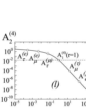
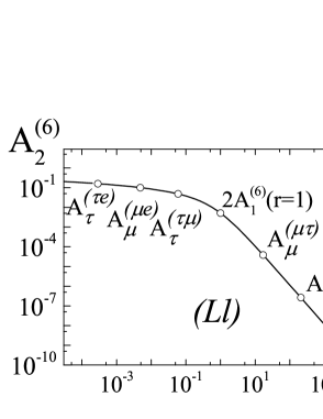
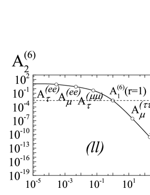
Figure 4: The fourth and sixth order coefficients $\displaystyle A_{2}^{(4)}(r)$ and $\displaystyle A_{2}^{(6)}(r)$, Eq. (31), as functions of the mass ratio $\displaystyle r=m_{\ell}/m_{L}$, for an external lepton $\displaystyle L$ with insertions of the polarization operators with one loop, left panel, and two loops, central and right panels. The notation corresponds to $\displaystyle A_{L}^{(\ell)}(r)$, $\displaystyle A_{L}^{(L\ell)}$, and $\displaystyle A_{L}^{(\ell\ell)}$, Eqs. (43), (56) and (50), respectively, where $\displaystyle L$ and $\displaystyle\ell=e,\mu,\tau$. The horizontal dashed lines indicate the values of the coefficients at $\displaystyle r=1$, i.e., the values $\displaystyle A_{1}^{(4)}$, Eq. (46), and $\displaystyle A_{1}^{(6)}$, Eq. (63), which are universal for any kind of the considered leptons. The central and right panels illustrate the same dependence of $\displaystyle A_{2}^{(6)}(r)$ but for the combinations $\displaystyle(L\ell)$, Eq. (56), and $\displaystyle(\ell\ell)$, Eqs. (50), respectively. The open circles, as well as the associated with them labels, point to physical values of the ratio $\displaystyle r$ and to the corresponding coefficients $\displaystyle A_{2}^{(\ell)}(r)$ or $\displaystyle A_{2}^{(L\ell)}(r)$.

In Fig. 4, we present the results of calculations of the fourth, $\displaystyle A_{2}^{(4)}(r)$, and sixth order corrections, $\displaystyle A_{2}^{(6)}(r)$, for diagrams with one and two lepton loops, as depicted in Fig. 2. The variable $\displaystyle r$ is defined as $\displaystyle r=m_{\ell}/m_{L}$ and varies in the interval $\displaystyle r\in(0,\infty)$. To ease the visibility of the results, the coefficients $\displaystyle A_{2}^{(4,6)}(r)$ for physical values of $\displaystyle r$, i.e., when $\displaystyle L$ and $\displaystyle\ell$ denote the real existing leptons $\displaystyle e,\mu$ and $\displaystyle\tau$, are marked in Fig. 4 by open circles. Moreover, for a better illustration of the combinations of $\displaystyle L$ and $\displaystyle\ell$, each physical value of $\displaystyle A_{2}^{(4,6)}(r)$ is additionally labeled by $\displaystyle A_{L}^{(\ell)}$ (left panel), $\displaystyle A_{L}^{(L\ell)}$ (central panel) and and $\displaystyle A_{L}^{(\ell\ell)}$ (right panel). Analogously, in Fig. 5 we present the results of calculations of the eighth order contributions from diagrams of three types: (i) insertions of three loops where one loop corresponds to the external (under consideration) lepton and two loops with lepton pairs different from the first one, i.e., diagrams of type $\displaystyle(L\ell\ell)$, left panel in Figs. 3 and 5 (ii) one lepton loop different from the external lepton, two other correspond to the external one, i.e., diagrams of the type $\displaystyle(LL\ell)$, central panel in Figs. 3 and 5, (iii) eventually, the diagrams with all three loops with leptons of the same type $\displaystyle(\ell\ell\ell)$, including also the case when $\displaystyle L=\ell$, right panel in Figs. 3 and 5.

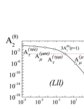
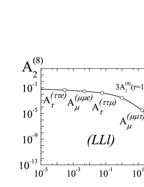
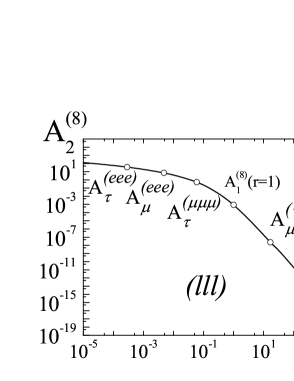
Figure 5: The eighth order coefficients $\displaystyle A_{2}^{(8)}(r)$, Eq. (31), as functions of the mass ratio $\displaystyle r=m_{\ell}/m_{L}$, for an external lepton $\displaystyle L=e,\mu,\tau$ with insertions of the polarization operators with three loops formed by leptons of different types. Left panel: the coefficients $\displaystyle A_{2}^{(8)}(r)$ determined by diagrams with three loops with one lepton as the external $\displaystyle L$ and two other different from $\displaystyle L$. The notation corresponds to $\displaystyle A_{L}^{(L\ell\ell)}(r)$, Eq. (58), where $\displaystyle L$ and $\displaystyle\ell=e,\mu,\tau$. The horizontal dashed line indicates the value of the coefficients at $\displaystyle r=1$, i.e., the coefficints $\displaystyle A_{1}^{(8)}$, Eq. (30) which are universal for any kind of the considered leptons. The central and right panels illustrate the same dependence of $\displaystyle A_{L}^{(L\ell\ell)}(r)$ but for the combinations $\displaystyle(LL\ell)$, Eqs. (64)-(67), and $\displaystyle(\ell\ell\ell)$, Eqs. (71)-(VI.3.2), respectively.

From Figs. 4 and 5 one infers that the radiative corrections decrease rather fast, by about 10-15 orders of magnitude, with increase of $\displaystyle r$ from its smallest to highest physical values. It means that the contribution of the heaviest $\displaystyle\tau$-lepton to the anomaly of the lighter ones is much smaller than the contribution from properly the muon and electron loops. This effect increases with increasing of order of the radiative corrections from $\displaystyle\alpha^{2}$ to $\displaystyle\alpha^{4}$ and depends on the combination of the internal and external leptons. However, due to the extremely high precision achieved in the measurements of the lepton anomalies Parker:2018vye ; Malaescu ; Davoudiasl:2018fbb ; E989 ; E821 , the corrections from $\displaystyle\tau$-leptons cannot be neglected. The horizontal dashed lines in Figs. 4 and 5 correspond to the values of the coefficients $\displaystyle A_{2}^{(4)-(8)}(r)$ at $\displaystyle r=1$, i.e., to the universal coefficients $\displaystyle A_{1}^{(4)-(8)}$, Eq. (30).

Another interesting circumstance to be stressed is that, according to Eq. (25), the radiative corrections are governed not only by the mass ratio $\displaystyle r$ but, at the same value of $\displaystyle r$, they are also quite sensitive to the combinations of $\displaystyle\Omega_{p}$ and $\displaystyle R_{j}$ in (25), i.e., to the concrete form of the Feynman diagram. Recall that $\displaystyle p+j=n$ and that $\displaystyle\Omega_{p}$ is determined by the $\displaystyle p-th$ power of the lepton polarization operator, while $\displaystyle R_{j}$ contains the imaginary part of the sum $\displaystyle\big{[}\Pi_{l}(t)+\Pi_{L}(t)\big{]}^{j}$, cf. Eqs. (26) and (18). So for the corrections to the electron anomaly at, e.g. $\displaystyle r=m_{\mu}/m_{e}$, one has $\displaystyle A_{e}^{ee\mu}(r)\gg A_{e}^{e\mu\mu}(r)\gg A_{e}^{\mu\mu\mu}(r)$ which vary from $\displaystyle A_{e}^{ee\mu}(r)\sim 2\cdot 10^{-7}$ to $\displaystyle A_{e}^{\mu\mu\mu}(r)\sim 2\cdot 10^{-12}$. The same situation occurs for $\displaystyle r=m_{e}/m_{\tau}$ as well as for muons and tauons. Qualitatively, the relative contributions of the three loop diagrams to the $\displaystyle e,\mu$ and $\displaystyle\tau$-leptons is illustrated in Fig. 6, where the corrections from different types of insertions decrease from left to right.

Figure 6: Qualitative illustration of the contributions to the eighth order coefficients $\displaystyle A_{2}^{(8)}(r)$, Eq. (31), of different types of Feynman diagrams, Fig. 3, in descending order: the upper row refers to electrons, the middle row to muons and the lower row to taons. The notation corresponds to $\displaystyle A_{L}^{(\ell\ell\ell)}(r)$, $\displaystyle A_{L}^{(LL\ell)}(r)$ and $\displaystyle A_{L}^{(L\ell\ell)}(r)$, where $\displaystyle L=e$ (upper row), $\displaystyle L=\mu$ (middle row), $\displaystyle L=\tau$ (lower row) and $\displaystyle\ell=e,\mu,\tau$.

Here it is appropriate to reiterate that the presented results demonstrate the qualitative analysis of the contribution of one, two and three loop diagrams to the lepton anomaly. For a scrupulous quantitative investigation of the considered radiative corrections one can use the exact analytical expressions reported above.

VII.1 The asymptotic expansions

The performed qualitative analysis can be be essentially relieved if, instead of the exact analytical formulae, one employs their asymptotic expansions. Such analyzes have been widely used in the literature Aguilar:2008qj by approximate calculations of the corresponding integrals (25) with preliminarily found asymptotic expansions of $\displaystyle\Omega_{p}(s)$ and $\displaystyle R_{j}(s)$. Explicitly, the corresponding expansions can be found in Refs. Aguilar:2008qj . In our case, as an additional check of the obtained analytical expressions, we compare our asymptotical expansions with the known results reported before by taking the limits $\displaystyle r\ll 1$ and $\displaystyle r\gg 1$ for the coefficients (31). We have found that $\displaystyle A_{2}^{(8),(L\ell\ell)}(r\ll 1)$, Eq. (58), $\displaystyle A_{2}^{(8),(LL\ell)}(r\ll 1)$, Eq. (64), and $\displaystyle A_{2}^{(8),(\ell\ell\ell)}(r\ll 1)$, Eq. (71), are entirely consistent with the corresponding expressions reported in Refs. Aguilar:2008qj ; Kurz:2016bau . For the sake of brevity, we do not present them here, mentioning only that such expansions work surprisingly well in a large interval of $\displaystyle r<1$, from $\displaystyle r\sim 0$ up to $\displaystyle r\sim 0.3-0.4$.

As for $\displaystyle r\gg 1$, the asymptotic expansion for $\displaystyle A_{2}^{(8)}(r)$ has not been considered insofar. For this reason below we write out explicitly our asymptotics, $\displaystyle r\gg 1$, of the coefficients $\displaystyle A_{2}^{(8),(L\ell\ell)}(r\gg 1)$, $\displaystyle A_{2}^{(8),(LL\ell)}(r\gg 1)$ and $\displaystyle A_{2}^{(8),(\ell\ell\ell)}(r\gg 1)$, cf. Eqs. (58), (VI.2.2) and (VI.3.2):

$$\displaystyle A_{2}^{(8),(L\ell\ell)}(r\gg 1)=\left[\frac{5809}{1080000}-\frac{61}{27000}\ln(r)+\frac{2}{225}\ln^{2}(r)\right]\frac{1}{r^{4}}+$$ (78)

$$\displaystyle\left[\frac{1862387}{277830000}-\frac{6073}{496125}\ln(r)+\frac{2}{175}\ln^{2}(r)\right]\frac{1}{r^{6}}+~{}~{}~{}~{}~{}~{}~{}~{}~{}~{}~{}~{}~{}~{}~{}$$

$$\displaystyle\left[\frac{12916049}{9001692000}-\frac{1940611}{100018800}\ln(r)+\frac{671}{7938}\ln^{2}(r)\right]\frac{1}{r^{8}}+{\cal O}\left(\frac{1}{r^{10}}\right)\,,$$

$$\displaystyle A_{2}^{(8),(LL\ell)}(r\gg 1)=\bigg{[}\frac{16}{45}\,\zeta(3)-\frac{203}{486}\bigg{]}\frac{1}{r^{2}}+\bigg{[}\frac{17}{105}\zeta(3)-\frac{40783}{2315250}\ln(r)-\frac{1023526159}{5186160000}$$ (79)

$$\displaystyle-\frac{37}{11025}\ln^{2}(r)-\frac{2}{315}\ln^{3}(r)\bigg{]}\frac{1}{r^{4}}+\bigg{[}-{\frac{1243103\,}{93767625}}\ln\left(r\right)-{\frac{4744350631}{472588830000}}+{\frac{8}{945}}\,\zeta\left(3\right)+$$

$$\displaystyle{\frac{2122\,}{297675}}\ln^{2}\left(r\right)-{\frac{16\,}{2835}}\ln^{3}\left(r\right)\bigg{]}\frac{1}{{r}^{6}}+\bigg{[}\frac{8}{2079}\zeta(3)-\frac{1013327141}{99843767100}\ln(r)-$$

$$\displaystyle{\frac{8721404003611}{2767669224012000}}+{\frac{166657}{14407470}}\ln^{2}(r)-{\frac{16}{6237}}\ln^{3}(r)\bigg{]}\frac{1}{r^{8}}+{\cal O}\left(\frac{1}{r^{10}}\right)\,,$$

$$\displaystyle A_{2}^{(8),(\ell\ell\ell)} \displaystyle(r\gg 1)=\bigg{[}\frac{87709}{9729720}-\frac{89}{15015}\zeta(3)\bigg{]}\frac{1}{r^{4}}+\bigg{[}\frac{12204667}{1824322500}-\frac{4}{1125}\ln(r)-\frac{40}{9009}\zeta(3)\bigg{]}\frac{1}{r^{6}}$$ (80)

$$\displaystyle+\bigg{[}\frac{73879547}{17721990000}-\frac{2}{375}\ln(r)-\frac{334}{109395}\zeta(3)\bigg{]}\frac{1}{r^{8}}+{\cal O}\left(\frac{1}{r^{10}}\right)\,.$$

NB: the asymptotics of the infinite sums $\displaystyle S_{2}(r)$, Eq. (67), and $\displaystyle S_{4}(r)$, Eq. (77), which, as mentioned, converge rapidly as $\displaystyle n\gg 1$, have been obtained by restricting the summation index $\displaystyle n$ to a finite value $\displaystyle N\sim 5000$ and then by taking the asymptotics $\displaystyle r\gg 1$.

Comparing the asymptotic expansion (78)-(80) with their corresponding exact expressions one concludes that (78)-(80) provide basically the same (numerical) results as the exact ones already starting from $\displaystyle r\sim 2\div 2.5\,$.

It is worth mentioning that in computing integrals of type (59), one obtains, depending on the method of integration used in dependence of the used, analytical results in terms of various special functions, viz. polygammas $\displaystyle\psi^{(n)}(r)$, polylogarithms $\displaystyle{\rm Li}_{n}(r)$, harmonic functions $\displaystyle H(n,r)$, Hurwits-Lerch transcendent $\displaystyle\Phi(r,n,a)$ etc. To reconcile different analytical results to each other, the number of special functions involved in integration must be maximally reduced by using the known relations among these special functions (see Appendix A). In such a way, the asymptotical expressions for $\displaystyle r\ll 1$ have been identically reduced to the previously reported expansions. This further persuades us of the correctness of our analytical analysis of the coefficients (30)-(31) and, consequently, that for each coefficient in Eq (31) there is a corresponding analytical function valid in the whole interval $\displaystyle r\in(0,\infty)$.

VIII Summary

In summary, we have presented an investigation of the contributions to the anomalous magnetic moment of leptons $\displaystyle L$ ($\displaystyle L=e\,,\,\mu$ or $\displaystyle\tau$) generated by QED diagrams with insertions of one, two and three loops in the photon vacuum polarization operator. We considered all possible combinations of external and internal leptons in the bubble-like diagrams. The radiative corrections for each diagram are obtained in close analytical forms. We argued that each coefficient $\displaystyle A_{2}(r)$ determining the corresponding $\displaystyle 4$th, $\displaystyle 6$th and $\displaystyle 8$th order of the radiative corrections can be represented explicitly by analytic functions which depend on the mass ratio $\displaystyle r=m_{l}/m_{L}$, being different for different combinations of the external $\displaystyle(L)$ and internal ($\displaystyle\ell$) leptons in the Feynman diagrams of the corresponding order. The generic variable $\displaystyle r$ of these functions is defined in the whole region $\displaystyle 0<r<\infty$.

Our consideration is based on a combined use of the dispersion relations for the vacuum polarization operators and the Mellin-Barnes integral transform for the Feynman parametric integrals. This technique is widely used in the literature in multi-loop calculations in relativistic quantum field theories, c.f. Refs. Friot:2005cu ; Rafael-HVP ; Kotikov:2018wxe . The ultimate integrations have been performed by the Cauchy residue theorem in the left ($\displaystyle r<1$) and right ($\displaystyle r>1$) semiplanes of the complex Mellin variable $\displaystyle s$. We demonstrate that the results in these two regions complement each other and determine the two branches of a common, for each considered Feynman diagram, analytical function. We investigated numerically the behaviour of these functions in the whole interval $\displaystyle 0<r<\infty$ and classified for each lepton the contribution of various diagrams in descending order of their significance. We also showed that the diagrams with $\displaystyle r>1$, i.e. diagrams with loops formed by heavier leptons, play a minuscule role in comparison with the role of corrections in the interval $\displaystyle r<1$. However, in high precision calculations such contributions can not be neglected.

Whenever pertinent, we compared our analytical expressions and the corresponding asymptotical expansions with well-known results available in the literature and found that they are fully compatible with the early known calculations.

The present paper can be considered as further developments of the efforts aimed at a better understanding of the role of bubble-like diagrams in the lepton anomaly and as an extension of previously reported analysis to the all three muons in the whole interval of the mass ratio $\displaystyle r$, $\displaystyle(0\,<\,m_{l}/m_{L}\,<\,\infty)$. The performed analysis persuades us that the Mellin-Barnes approach probably can be successfully applied in calculating analogous diagrams with insertions, this time, of hadron loops in the polarization operator.

Appendix A Some useful relations

Direct employment of the Cauchy residue theorem to the integrals, Eqs. (40), (50), (53), (57), (59), and (68) results in expressions containing a variety of special functions, viz. polygammas $\displaystyle\psi^{(m)}(n)$, polylogarithms $\displaystyle{\rm Li}_{n}(r)$, generalized harmonic functions $\displaystyle H_{n}^{(m)}$, Hurwits-Lerch transcendent $\displaystyle\Phi(r,n,a)$ etc. Using the herebelow relations, the number of necessary special functions can be essentially reduced. This allows one to reconcile explicitly our results to the ones known in the literature and reported in different forms with different special functions, cf. Refs. Friot:2005cu ; Laporta:1993ju ; Sidorov:2019 . Also, by using the appropriate properties of the remaining functions for $\displaystyle r<1$ and $\displaystyle r>1$, one can express the corresponding coefficients $\displaystyle A_{2}(r<1)$ through the coefficients $\displaystyle A_{2}(r<1)$, which allows one to assert that there exist, for each Feynman diagram, a common analytical function valid in the whole interval $\displaystyle(0\,<\,r\,\infty)$.

$$\displaystyle\begin{array}[]{lr}\Phi(r,2,1/2)=\frac{2}{\sqrt{r}}\left[{\rm{Li}_{2}}(\sqrt{r})-{\rm{Li}_{2}}(-\sqrt{r})\right];\\[8.53581pt] \Phi(r,2,3/2)=-\frac{4}{r}+\frac{2}{r\sqrt{r}}\left[{\rm{Li}_{2}}(\sqrt{r})-{\rm{Li}_{2}}(-\sqrt{r})\right];\\[8.53581pt] \Phi(r,2,5/2)=-\frac{4}{9r}-\frac{4}{r^{2}}+\frac{2}{r^{2}\sqrt{r}}\left[{\rm{Li}_{2}}(\sqrt{r})-{\rm{Li}_{2}}(-\sqrt{r})\right];\\[8.53581pt] {\rm{Li}_{2}}(1-r)+{\rm{Li}_{2}}\left(1-\frac{1}{r}\right)=-\frac{1}{2}\ln^{2}(r);\qquad\qquad{\rm(r>0)};\\[8.53581pt] {\rm{Li}_{2}}(r)+{\rm{Li}_{2}}(1/r)=-\frac{\pi^{2}}{6}-\frac{1}{2}\ln^{2}(-r);\qquad\qquad{\rm(r>1)};\\[8.53581pt] {\rm{Li}_{3}}(r)-{\rm{Li}_{3}}(1/r)=-\frac{\pi^{2}}{6}\ln(-r)-\frac{1}{6}\ln^{3}(-r);\qquad{\rm(r>1)}\\[8.53581pt] {\rm{Li}_{3}}(r)-{\rm{Li}_{3}}(1/r)=\frac{\pi^{2}}{6}\ln(-1/r)+\frac{1}{6}\ln^{3}(-1/r);\qquad{\rm(r<1)}\\[8.53581pt] {\rm{Li}_{4}}(r)+{\rm{Li}_{4}}(1/r)=-\frac{7\pi^{4}}{360}-\frac{\pi^{2}}{12}(\ln(-r))^{2}-\frac{1}{24}\ln^{4}(-r);\qquad\qquad{\rm(r>1)}\\[8.53581pt] {\rm Li_{2}}\left(\frac{1-r}{1+r}\right)-{\rm Li_{2}}\left(-\frac{1-r}{1+r}\right)={\rm Li_{2}}(-r)-{\rm Li_{2}}(r)+\bigg{(}\ln(1+r)\ln(r)-\ln(1-r)\bigg{)}\ln(r)+\frac{\pi^{2}}{4};\\[14.22636pt] {\rm Li_{n}}(r)+{\rm Li_{n}}(-r)=\frac{1}{2^{n-1}}{\rm Li_{n}}(r^{2}).\\[8.53581pt] \end{array}$$ (91)

$$\displaystyle{\rm arctanh(r)}=\frac{1}{2}\bigg{[}\ln(1+r)-\ln(1-r)\bigg{]};$$ (92)

$$\displaystyle{\rm H_{n}^{(1)}}=\psi^{(1)}(n+1)+\gamma;\quad{\rm H}_{n}^{(2)}=\frac{\pi^{2}}{6}-\psi^{(1)}(n+1),$$ (93)

where $\displaystyle{\rm Li_{n}}(r)$, $\displaystyle\Phi(r,s,a)$, $\displaystyle{\rm H_{n}^{(m)}}$ and $\displaystyle\psi^{(m)}(n)$ are the polylogaritm, Lerch transcendent, generalized harmonic number and Euler polygamma functions, respectively.

References

• (1) P. A. M. Dirac, The quantum theory of the electron, Proc. Roy. Soc. Lond. A 117, 619 (1928).
• (2) T. Aoyama et al., The anomalous magnetic moment of the muon in the Standard Model, Phys. Rep. 887, 1 (2020).
• (3) F. Jegerlehner, The anomalous magnetic moment of the muon, Springer Tracts Mod. Phys.  274, 693 (2017).
• (4) R. H. Parker, C. Yu, W. Zhong, B. Estey, H. M$\displaystyle\ddot{u}$eller, Measurement of the fine-structure constant as a test of the Standard Model, Science 360, 191 (2018).
• (5) B. Abi et al., [Muon $\displaystyle g-2$ Coll.], Measurement of the positive muon anomalous magnetic moment to 0.46 ppm, Phys. Rev. Lett. 126, 141801 (2021).
• (6) G. W. Bennett, Final report of the muon E821 anomalous magnetic moment measurement at BNL, Phys. Rev. D 73, 072003 (2006).
• (7) A. Keshavarzi, D. Nomura, T. Teubner, $\displaystyle g-2$ of charged leptons, $\displaystyle\alpha(M_{Z}^{2})$ and the hyperfine splitting of muonium, Phys. Rev. D 101, 014029 (2020).
• (8) A. Keshavarzi, W. J. Marciano, M. Passera and A. Sirlin, Muon $\displaystyle g-2$ and $\displaystyle\Delta\alpha$ connection, Phys. Rev. D 102, 033002 (2020).
• (9) M. Davier, A. Hoecker, B. Malaescu, Z. Zhang, A new evaluation of the hadronic vacuum polarisation contributions to the muon anomalous magnetic moment and to $\displaystyle\alpha(m_{Z}^{2})$, Eur. Phys. J. C 80, 241 (2020), Erratum: [Eur. Phys. J. C 80, 410 (2020)].
• (10) H. Davoudiasl, W. J. Marciano, Tale of two anomalies, Phys. Rev. D 98, 075011 (2018).
• (11) G. Colangelo, M. Hoferichter, P. Stoffer, Two-pion contribution to hadronic vacuum polarization, JHEP 02, 006. arXiv: 1810.00007 [hep-ph] (2019).
• (12) M. Hoferichter, B.-L. Hoid, B. Kubis. Three-pion contribution to hadronic vacuum polarization. JHEP 08, 137. arXiv: 1907.01556 [hep-ph] (2019).
• (13) S. Borsanyi et al., Leading hadronic contribution to the muon magnetic moment from lattice QCD, Nature 593, 51 (2021); arXiv:2002.12347 [hep-lat].
• (14) G. Colangelo, A.X. El-Khadra, M. Hoferichter, A. Keshavarzi, C. Lehner, P. Stoffer, T. Teubner, Data driven evaluations of Euclidean windows to scrutinixe hadronic vacuum polarizatiom, Phys. Lett. B 833, 137313 (2022).
• (15) G. Colangelo, M. Davier, A.X. El-Khadra, M. Hoferichter, C. Lehner et al., Prospects for precise predictions of $\displaystyle a_{\mu}$ in the Standard Model, Contribution to 2022 Snowmass Summer Study; arXiv: 2203.15810 [hep-ph] (2022).
• (16) M. Cé, A. Gérardin, G. von Hippel, R. J. Hudspith, S. Kuberski et al., Window observable for the hadronic vacuum polarization contribution to the muon $\displaystyle g-2$ from lattice QCD arXiv: 2206.06582 [hep-lat] (2022).
• (17) J. Grange et al., [Muon $\displaystyle g-2$ Collaboration], Muon $\displaystyle(g-2)$ technical design report, arXiv:1501.06858 [physics.ins-det];
A. Keshavarzi [Muon g-2 Collaboration], The muon $\displaystyle g-2$ experiment at Fermilab, EPJ Web Conf.  212, 05003 (2019).
• (18) H. Iinuma [J-PARC muon $\displaystyle g-2$/EDM Collaboration], New approach to the muon $\displaystyle g-2$ and EDM experiment at J-PARC, J. Phys. Conf. Ser.  295, 012032 (2011).
• (19) J. S. Schwinger, On quantum electrodynamics and the magnetic moment of the electron, Phys. Rev.  73, 416 (1948).
• (20) T. Kinoshita, B. Nizic, Y. Okamoto, Eighth order QED contribution to the anomalous magnetic moment of the muon, Phys. Rev.  D 41, 593 (1990).
• (21) S. Laporta, The analytical contribution of the sixth order graphs with vacuum polarization insertions to the muon $\displaystyle(g-2)$ in QED, Nuovo Cim. A 106, 675 (1993).
• (22) S. Laporta, The analytical contribution of some eighth order graphs containing vacuum polarization insertions to the muon $\displaystyle(g-2)$ in QED, Phys. Lett. B 312, 495 (1993).
• (23) T. Kinoshita, M. Nio, Improved $\displaystyle\alpha^{4}$ term of the electron anomalous magnetic moment, Phys. Rev. D 73, 013003 (2006).
• (24) S. Laporta, High-precision calculation of the 4-loop contribution to the electron $\displaystyle g-2$ in QED, Phys. Lett. B 772, 232 (2017).
• (25) J. P. Aguilar, D. Greynat, E. de Rafael, Muon anomaly from lepton vacuum polarization and the Mellin-Barnes representation, Phys. Rev.  D 77, 093010 (2008).
• (26) A. Kurz, T. Liu, P. Marquard, M. Steinhauser, Anomalous magnetic moment with heavy virtual leptons, Nucl. Phys. B 879, 1 (2014).
• (27) A. Kurz, T. Liu, P. Marquard, A. Smirnov, V. Smirnov, M. Steinhauser, Electron contribution to the muon anomalous magnetic moment at four loops, Phys. Rev. D 93, 053017 (2016).
• (28) P. A. Baikov, A. Maier, P. Marquard, The QED vacuum polarization function at four loops and the anomalous magnetic moment at five loops, Nucl. Phys. B 877, 647 (2013).
• (29) P. Marquard, A. V. Smirnov, V. A. Smirnov, M. Steinhauser, D. Wellmann, $\displaystyle(g-2)_{\mu}$ at four loops in QED, arXiv:1708.07138. [hep-ph].
• (30) S. Friot, D. Greynat, E. de Rafael, Asymptotics of Feynman diagrams and the Mellin-Barnes representation, Phys. Lett. B 628, 73 (2005).
• (31) R. Z. Roskies, Comptational aspects of quantum electrdynamics: the lepton factors, AIP Conf. Proc. 23, 376 (1975); https://doi.org/10.1063/1.2947439.
• (32) V. B. Berestetskii, O. N. Krohnin, A. K. Khlebnikov, Concerning the radiative corrections to the $\displaystyle\mu$-meson magnetic moment, Zh. Eksp. Teor. Fiz., 30, 788 (1956) [Sov. Phys. JETP, 3, 761 (1956)].
• (33) S. J. Brodsky, E. de Rafael, Suggested boson-lepton pair coupling and the anamalous magnetic moment of the muon, Phys. Rev. 168, 1620 (1968).
• (34) S. Friot, D. Greynat, On convergent series representations of Mellin-Barnes integrals, J. Math. Phys.  53, 023508 (2012).
• (35) J. Charles, E. de Rafael, D. Greynat, Mellin-Barnes approach to hadronic vacuum polarization and $\displaystyle g_{\mu}-2$, Phys. Rev. D 97, 076014 (2018).
• (36) B. Ananthanarayan, S. Friot, S. Ghosh, Three-loop QED contributions to the $\displaystyle g-2$ of charged leptons with two internal fermion loops and a class of Kampe de Feriet series, Phys. Rev. D 101, 116008 (2020).
• (37) E. E. Boos, A. I. Davydychev, A method of evaluation massive Feynman diagrams, Theor. Math. Phys. 89, 1052 (1991) [Theor. Math. Fiz. 89, 56 (1991)].
• (38) M. L. Laursen, M. A. Samuel, The $\displaystyle n$-bubble diagram contribution to $\displaystyle g-2$ of the electron mathematical structure of the analytical expression, Phys. Lett.  91B, 249 (1980); The $\displaystyle n$-bubble diagram contribution to $\displaystyle g-2$, J. Math. Phys.  22, 1114 (1981).
• (39) A. Petermann, Fourth order magnetic moment of the electron, Helv. Phys. Acta 30, 407 (1957).
• (40) C. M. Sommerfield, Magnetic dipole moment of the electron, Phys. Rev.  107, 328 (1957).
• (41) S. Laporta, E. Remiddi, The analytical value of the electron $\displaystyle(g-2)$ at order $\displaystyle\alpha^{3}$ in QED, Phys. Lett. B 379, 283 (1996).
• (42) S. Laporta, New results on $\displaystyle g-2$ calculation, J. Phys. Conf. Ser.  1085, no. 2, 022004 (2018); Four-loop QED contributions to the electron $\displaystyle g-2$, J. Phys. Conf. Ser.  1138, no. 1, 012001 (2018).
• (43) B. E. Lautrup, On high order estimates in QCD, Phys. Lett. B 69, 109 (1977).
• (44) S. Eidelman, M. Passera, Theory of the tau lepton anomalous magnetic moment, Mod. Phys. Lett. A 22, 159 (2007); e-Print: hep-ph/0701260 [hep-ph].
• (45) B. E. Lautrup, E. de Rafael, Calculation of the sixth-order contribution from the fourth-order vacuum polarization to the difference of the anomalous magnetic moments of muon and electron, Phys. Rev.  174, 1835 (1968).
• (46) H. Suura, E.H. Wichmann, Magnetic moment of the mu meson, Phys. Rev. 105, 1930 (1957).
• (47) G. Li, R. Mendel, M. A. Samuel, Precise mass ratio dependence of fourth order lepton anomalous magnetic moments: The effect of a new measurement of $\displaystyle m_{\tau}$, Phys. Rev. D 47, 1723 (1993).
• (48) A. Czarnecki, M. Skrzypek, The muon anomalous magnetic moment in QED: three loop electron and tau contributions, Phys. Lett. B 449, 354 (1999).
• (49) A. V. Kotikov, S. Teber, Multi-loop techniques for massless Feynman diagram calculations, Phys. Part. Nucl. 50, no.1, 1 (2019) [arXiv:1805.05109 [hep-th]].
• (50) O. P. Solovtsova, V. I. Lashkevich, A. V. Sidorov, Some analytic results for the contribution to the anomalous magnetic moments of leptons due to the polarization of vacuum via lepton loops, EPJ Web of Conferences 222, 03007 (2019).