MovieCLIP: Visual Scene Recognition in Movies

Abstract

Longform media such as movies have complex narrative structures, with events spanning a rich variety of ambient visual scenes. Domain specific challenges associated with visual scenes in movies include transitions, person coverage, and a wide array of real-life and fictional scenarios. Existing visual scene datasets in movies have limited taxonomies and don’t consider the visual scene transition within movie clips. In this work, we address the problem of visual scene recognition in movies by first automatically curating a new and extensive movie-centric taxonomy of 179 scene labels derived from movie scripts and auxiliary web-based video datasets. Instead of manual annotations which can be expensive, we use CLIP to weakly label 1.12 million shots from 32K movie clips based on our proposed taxonomy. We provide baseline visual models trained on the weakly labeled dataset called MovieCLIP and evaluate them on an independent dataset verified by human raters. We show that leveraging features from models pretrained on MovieCLIP benefits downstream tasks such as multi-label scene and genre classification of web videos and movie trailers.

1 Introduction

Media, in its diverse forms and modalities, is used to create and share narratives across domains including movies, television shows, advertisements, games, news, and user generated social stories. Movies represent a major form of media content, with box office revenues estimated at $4.48 billion across 329 movies released in 2021 [37], with a global reach and societal influence.

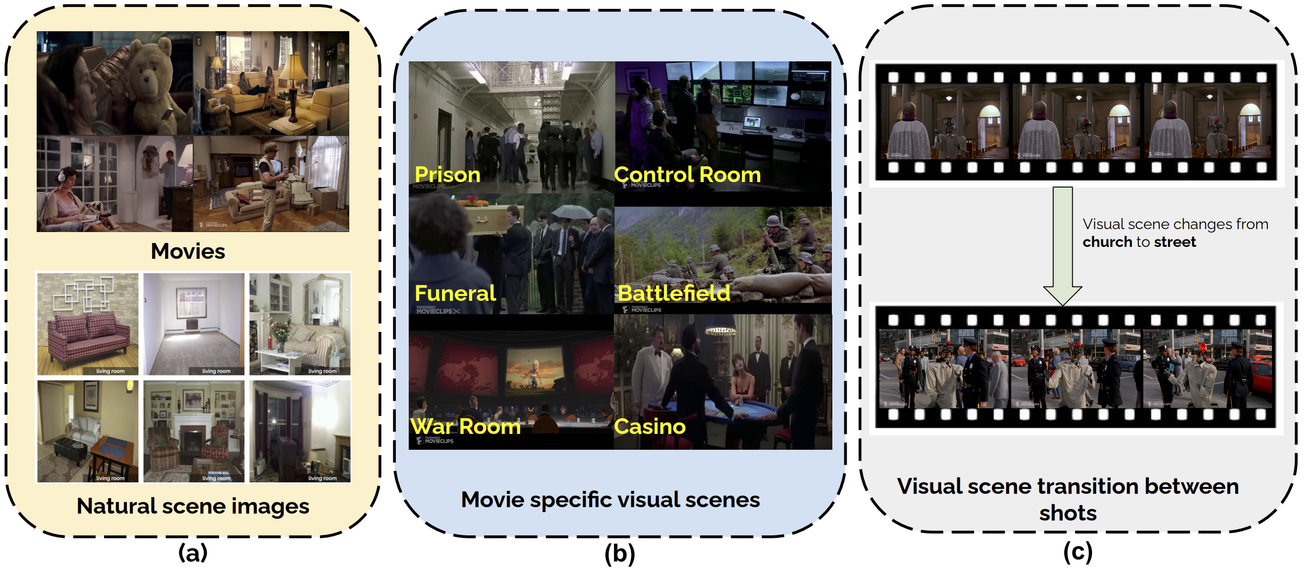
Figure 1: Overview diagram highlighting the challenges associated with visual scene recognition in movies (a) Domain mismatch between Natural scene images,(Source: http://places2.csail.mit.edu/explore.html) vs frames from Movies for living room (b) Movie centric visual scene classes like prison, control room etc that are absent from existing taxonomies (c) Change in visual scene between shots in the same movie clip.

The computational analysis of media content [49] especially movies presents unique challenges due to their long-form narrative structures with character interactions often spanning diverse visual scenes and contexts. In cinematic terms, mis-en-scene [4] refers to how the different elements of a film are depicted and arranged in front of camera. Key components of mis-en-scene include the actors with their different styles, visual scenes where the interactions take place, set design including lighting and camera placement and the accompanying costumes and makeup of the artists. The visual scene is considered a crucial component since it sets the mood and provides a background for the various actions performed by the actors in the scene. Visual scenes in movies are often tied to social settings like weddings, birthday parties and workplace gatherings that provide information about character interactions.

Accurate recognition of visual scenes can help in uncovering the bias involved in portrayal of under-represented characters vis-a-vis different scenes e.g., fewer women shown in office as compared to kitchen. For content tagging tasks like genre classification, visual scenes provide context information like battlefield portrayals in action/adventure movies, space-shuttle in sci-fi movies or courtrooms in dramas. However, there are certain inherent challenges in visual scene recognition for movies that needs to be addressed, as shown in Fig. 1:
Domain mismatch - scene images vs movie frames: Visual scenes depicted in movies are distinct compared to natural scenes due to increased focus on actors, multiple activities and viewpoint variations like extreme closeup, wide angle shots etc. An example is shown in Fig. 1 (a) for images from Places2 dataset [57] and movie frames from Condensed Movies dataset [1].
Lack of completeness in scene taxonomy: Movies depict both real life and fictional scenarios that span a wide variety of visual scenes. As shown in Fig. 1(b), certain movie centric visual scene classes like battlefield, control room, prison, war room, funeral, casino are absent from existing public scene taxonomies associated with natural scene image and video datasets.
Lack of shot specific visual scene annotations: Existing datasets like Condensed Movies [1] and VidSitu [46] provide a single visual scene label for the entire movie clip (around 2 minutes long), obtained through descriptions provided as part of YouTube channel Fandango Movie clips . In Fig. 1 (c), the provided description: Johnny Five (Tim Blaney) searches for his humanity in the streets of New York. mentions only the visual scene street, while the initial set of events takes place inside church. Instead of considering a single scene label for the entire movie clip, shot level visual scene annotation can help in tracking the scene change from church to street.

In our work, we consider shots within a given movie clip as the fundamental units for visual scene analysis since shots consist of consecutive set of frames related to the same content, whose starting and ending points are triggered by recording using a single camera [25]. Our contributions are as follows:

• Movie-centric scene taxonomy: We develop a movie-centric scene taxonomy by leveraging scene headers (sluglines) from movie scripts and existing video datasets with scene labels like HVU[13].

• Automatic shot tagging: We utilize our generated scene taxonomy to automatically tag around 1.12M shots from 32K movie clips using CLIP [41] based on a frame-wise aggregation scheme.

• Multi-label scene classification: We develop multi-label scene classification baselines using the shot-level tagged dataset called MovieCLIP and evaluate them on an independent shot level dataset curated by human experts. The dataset and associated codebase can be accessed at https://sail.usc.edu/mica/MovieCLIP/

• Downstream tasks: We further extract feature representations from the baseline models pretrained on MovieCLIP and explore their applicability in diverse downstream tasks of multi-label scene and movie genre classification from web videos [13] and trailers [9], respectively.

2 Related work

Image datasets for visual scene recognition: Image datasets for scene classification like MIT Indoor67 [40] relied on categorizing a finite set of (67) indoor scene classes. A broad categorization into indoor, outdoor (natural) and outdoor (man-made) groups for 130K images across 397 subcategories was introduced by the SUN dataset [56]. For large scale scene recognition, the Places dataset [57] was developed with 434 scene labels spanning 10 million images. The scene taxonomy considered in Places dataset was derived from the SUN dataset, followed by careful merging of similar pairs. It should be noted that the curation of large scale visual scene datasets like Places relied on crowd-sourced manual annotations over multiple rounds.
Video datasets for visual scene recognition: While there has been considerable progress in terms of action recognition capabilities from videos due to introduction of large scale datasets like Kinetics [28], ActivityNet [16], AVA [22], Something-Something [21], only few large scale datasets like HVU [13] and Scenes, Objects and Actions (SOA) [43] have focused on scene categorization with actions and associated objects. SOA was introduced as a multi-task multi-label dataset of social-media videos across 49 scenes with objects and actions but the taxonomy curation involves free-form tagging by human annotators followed by automatic cleanup. HVU [13], a recently released public dataset of web videos with 248 scene labels, relied on initial tag generation based on cloud APIs followed by human verification.
Movie-centric visual scene recognition: In the domain of scene recognition from movies, Hollywood scenes [36] was first introduced with 10 scene classes extracted from headers in movie scripts across 3669 movie clips. A socially grounded approach was explored in Moviegraphs [54] with emphasis on the underlying interactions (relationships/situations) along with spatio-temporal localizations and associated visual scenes (59 classes).

Dataset	Domain	#classes	#samples	Annotation	Unit	AV
Scene 15 [18]	Natural	15	$\sim$6k	Manual	Image	✓
MITIndoor67 [40]	Natural	67	15620	Manual	Image	✓
SUN397 [56]	Natural	397	130,519	Manual	Image	✓
Places [57]	Natural	434	10m	Manual	Image	✓
Hollywood Scenes [36]	Movies	10	3669	Automatic	Video clip (36.1s)	✓
Moviegraphs [54]	Movies	59	7637	Manual	Video clip (44.28 s)	✗
SOA [43]	Web-Videos	49	562K	Semi-automatic	Video clip (10 s)	✗
Movienet [27]	Movies	90	42K	Manual	Scene segment (2 min)	✗
HVU [13]	Web-Videos	248	251k	Semi-automatic	Video clip (10 s)	✓
Condensed Movies [1]	Movies	NA	33k	Automatic	Video clip ( 2 min)	✓
VidSitu [46]	Movies	$\sim$50	14k	Manual	Video clip (10 s)	✓
LVU [55]	Movies	6	723	Automatic	Video clip ($1\sim 3$ min)	✓
MovieCLIP	Movies	179	1.12m	Automatic	Shot (3.54s)	✓

Table 1: Comparison of MovieCLIP with other available image and video datasets with visual scene classes. Natural: Images of natural scenes.Web-Videos: videos obtained from internet sources like YouTube. AV: whether publicly available or not. Avg or duration span of video data sources are provided with the respective units. NA: Number of scene classes explicitly not mentioned with the dataset.

For holistic movie understanding tasks, the Movienet dataset[27] was introduced with the largest movie-centric scene taxonomy consisting of 90 place (visual scene) tags with segment wise human annotations of entire movies. Instead of entire movie data, short movie clips sourced from YouTube channel of Fandango Movie clips were used for text-video retrieval in Condensed movies dataset [1], visual semantic role labeling [46] and pretraining object-centric transformers [53] for long-term video understanding in LVU dataset [55]. While there is no explicit visual scene labeling, the raw descriptions available on Youtube with the movie clips have mentions of certain visual scene classes.
MovieCLIP, our curated dataset, is built on top of movie clips available as a part of Condensed Movies dataset [1]. A comparative overview of MovieCLIP and other image and video datasets with visual scene labels is shown in Table 1. In comparison with previous video-centric works, our taxonomy generation relies on domain-centric data sources like movie scripts and auxiliary world knowledge from web-video based sources like HVU with minimal human-in-the loop supervision for taxonomy refinement.
Knowledge transfer from pretrained vision language models: Vision language(V-L) based pretraining methods involve learning transferable visual representations based on various pretext tasks associated with image and text pairs. Examples of pretext tasks in V-L domain include prediction of masked words in captions based on visual cues in ICMLM [47], pretraining image encoders based on bicaptioning objective in VirTex [12] and contrastive alignment of image-caption pairs in CLIP [41]. Leveraging features from CLIP’s visual and text encoders have improved existing vision-language tasks [48] and enabled open-vocabulary object detection [23], and language driven semantic segmentation [32]. In our work, we use the pretrained visual and text encoders of CLIP and utilize it as a noisy annotator by tagging movie shots based on our curated visual scene taxonomy.

3 Taxonomy curation for movie scenes

In this section we outline the process involved in curating a visual scene taxonomy based on the domain information present in movie scripts and the pre-existing scene information present in auxiliary video datasets.

3.1 Sources of visual scene information

Movie scripts have been used as external sources for describing and annotating videos through script and subtitle alignment methods in [10], [15], [31], [45]. Movie scripts contain sluglines that provide information about visual scene, time of the day, and whether the action takes place in indoor or outdoor settings. Sample example of a slugline with visual scene as river is : EXT. GOTHAM RIVER - DAY. We parse 156k sluglines from a in-house set of 1434 movie scripts. For each slugline, we automatically extract entities after the ‘‘EXT.’’(exterior) or ‘‘INT.’’(interior) tags like Hospital room, River, War room etc. Using this procedure, we extract 173 unique visual scene labels. Since our taxonomy generation process is motivated by visual scenes in movies with sluglines from scripts as seed sources along with auxiliary sources. Since the set of labels from movie scripts is not exhaustive, we also consider auxiliary sources especially web video datasets with visual scene labels like HVU [13]. We consider HVU as source of additional labels since the taxonomy (248 visual scene classes) is semi-automatically curated for short-trimmed videos, having similar nature to movie shots. We don’t consider Places2 [57] dataset since the taxonomy is primarily curated for natural scenes, which are distinct from movie-centric visual scenes.

3.2 Visual scene taxonomy curation

In order to develop a comprehensive taxonomy of visual scenes in movies, we develop an automatic way of merging taxonomies from movie sluglines and the auxiliary dataset i.e., HVU with minimal human-in-the-loop for post-processing. The broad steps involved in the taxonomy generation are listed as below:

Label space preprocessing: For simplicity, we consider the set of unique labels from movie sluglines (MS) to be denoted as $L_{MS}$ and its cardinality as $N_{MS}$. Similarly we denote $N_{HVU}$ to be the cardinality of the set $L_{HVU}$, i.e., the set of unique labels from the HVU dataset. For our case, we have $N_{MS}=173$ and $N_{HVU}=248$. We extract the intersecting set of labels between $L_{MS}$ and $L_{HVU}$, denoted by the set $L_{com}$ . The number of common labels between HVU and movie slugline based taxonomy is $N_{com}=68$. We remove the common set of labels $L_{com}$ from both the label spaces of movie sluglines and HVU. This gives us a non-intersecting set of labels in movie sluglines and HVU denoted by $L_{MS}\setminus L_{Com}$ and $L_{HVU}\setminus L_{Com}$ respectively. We combine the sets of labels i.e. $L_{MS}\setminus L_{Com}$ and $L_{HVU}\setminus L_{Com}$ to obtain a larger set of labels called $L_{NC}$, where NC refers to not common.

$$L_{NC}=(L_{MS}\setminus L_{Com})\cup(L_{HVU}\setminus L_{Com})$$ (1)

Merging with common label space: In this step, we find labels in $L_{NC}$ that are semantically close to the labels in $L_{com}$. We extract dense 384D label representations using the MiniLM-L6-v2 sentence transformers model [44] for labels in $L_{NC}$ and $L_{com}$. For each label in $L_{NC}$ we compute cosine similarities with set of labels in $L_{com}$ based on label representations. We merge those labels from $L_{NC}$ with the similar labels in $L_{com}$, whose top-1 cosine similarity values are greater than 0.6. We update the set of labels $L_{NC}$ to $L_{N}$ by removing the merged labels. Examples of such merging with respective cosine similarities and sources are as follows:

• $\textbf{dune}\{L_{NC}\}\rightarrow{}\textbf{desert}\{L_{com}\}(0.66)$

• $\textbf{tennis}\ camp\{L_{NC}\}\rightarrow{}\textbf{tennis \ court}\{L_{com}\}(0.62)$

• $\textbf{restroom}\{L_{NC}\}\rightarrow{}\textbf{bathroom}\{L_{com}\}(0.80)$

• $\textbf{rural \ area}\{L_{NC}\}\rightarrow{}\textbf{village}\{L_{com}\}(0.64)$

• $\textbf{boardwalk}\{L_{NC}\}\rightarrow{}\textbf{walkway}\{L_{com}\}(0.67)$

• $\textbf{television \ room}\{L_{NC}\}\rightarrow{}\textbf{living \ room}\{L_{com}\}(0.67)$

• $\textbf{glacial \ lake}\{L_{NC}\}\rightarrow{}\textbf{lake}\{L_{com}\}(0.73)$

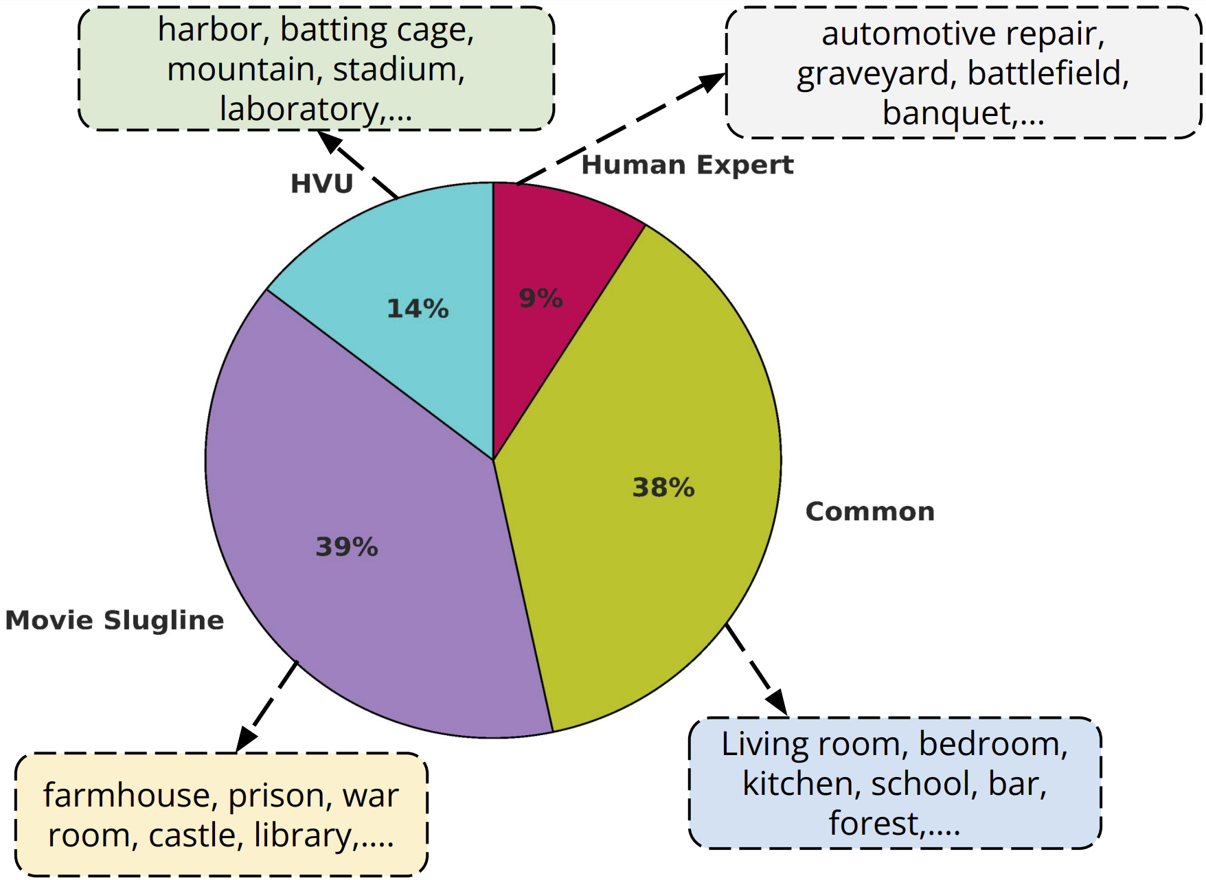
Figure 2: The share of different sources (HVU, Movie Sluglines, Common labels and Human expert) in curating the label taxonomy. Example labels from different sources are shown in boxes with the pie chart.

Human-in-the-loop taxonomy refinement: A human expert inspects the labels in $L_{N}$ and removes both generic scene labels such as body of water, coastal and oceanic landforms, horizon, landscape, underground as well as highly specific scenes such as coral reef, white house, piste, badlands etc. We use label representations from the previous step to exploit semantic similarity between the labels remaining in $L_{N}$. For each relevant label in $L_{N}$, a threshold of 0.7 on top-1 similarity score is used to filter out similar labels. While comparing two similar labels, the human expert relies on wiki definitions to merge the more specific label into the generic one. For example, by definition bazaar is a special form of market selling local items (as per wiki) and therefore merged with the market. Other examples include:

• $\{stream,riverbed,creek,river\}\rightarrow{}river$

• $\{hill,mountain,mountain\ pass,mountain\ range\}\\ \rightarrow{}mountain$

• $\{road,road\ highway,lane\}\rightarrow{}road$

• $\{port,marina\ dock,harbor\}\rightarrow{}harbor$

This results in a set of labels called $L_{merge}$ from $L_{N}$. Further, The human expert is exposed to randomly sampled 1000 shots from movie clips in Condensed Movies [1] and reviews the current set of labels in the set $L_{merge}\cup L_{com}$. Based on the video content, a set of scene labels ($L_{human}$) that are missing from the current set is added by human expert. Thus the final set of 179 visual scene labels is obtained as follows:

$$L_{final}=L_{com}\cup L_{merge}\cup L_{human}$$ (2)

Label source distribution: As shown in Fig. 2, the largest share is from movie sluglines (39%).Only 9% of the total labels is provided through feedback from human expert. Instead of manually binning classes into broad categories like indoor, outdoor or man-made, we discover groupings among classes through Affinity propagation clustering [20] (based on label representations from sentence transformers). Certain clusters of visual scene labels are listed below, where all the sport locations, water bodies and performing arts locations are grouped together.

• sport locations: Basketball court, Race track, Tennis court, Batting cage, Golf course

• water bodies: River, Pool, Waterfall, Hot spring, Pond, Swamp, Lake

• performing arts locations: Stage, Conference Room, Theater, Auditorium, Ballroom

• Natural landforms: Mountain, Desert, Valley

A detailed list of the clusters discovered among the visual scene classes is shown in Supplementary.

4 MovieCLIP dataset

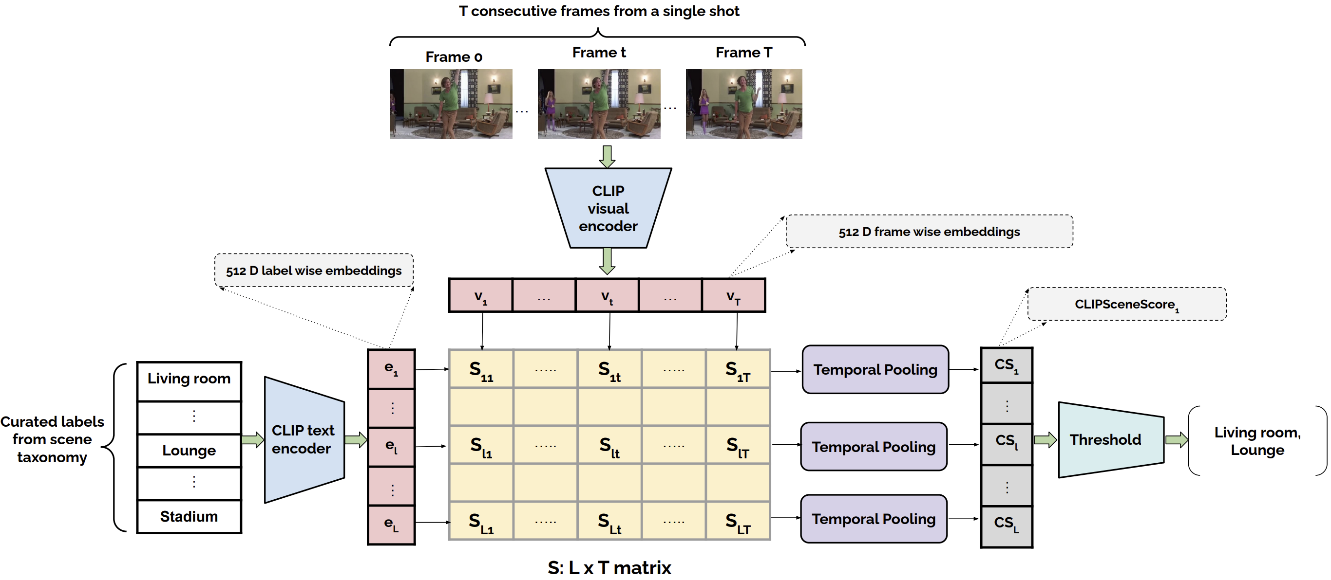
Figure 3: Overview schematic of the prompt based visual scene labeling of movie shot using CLIP’s visual and text encoders. $S$ is the similarity matrix where entry $S_{lt}$ refers to similarity values between textual embedding $e_{l}$ and visual embedding $v_{t}$.

We use the curated taxonomy described in Section 3 to develop a labeled dataset of movie shots called MovieCLIP. We outline the process of shot detection and automatic labeling using CLIP [41] in the following sections:

4.1 Shot detection from movie clips

Since a shot represents a continuous set of frames with minimal change in the visual scene, we consider movie shots for our subsequent analysis. Associating visual scene labels to shots can help in identifying cases where visual scene recognition is difficult like closeup or extreme closeup scenarios, even within the same movie scene. A singular movie scene involves changes in camera viewpoints across consecutive shots, thus making it difficult for CLIP to associate labels with high confidence for the entire movie scene. For shot detection, we use PySceneDetect to segment the movie clips in Condensed Movies with default parameters and content-aware detection mode. The overall statistics of the shot extraction process is shown in Table 2:

# movies	Years	# clips	# shots	Avg shots/clip	Avg Duration
3574	1930-2019	32484	1124638	34.66	3.54s

Table 2: Statistics of movie shots in MovieCLIP dataset.

4.2 CLIP based visual scene labeling of movie shots

In this section, we describe how CLIP [41] can be used to associate visual scene labels with individual movie shots. Since CLIP has been trained in a contrastive manner for alignment, it can be used to develop zero-shot classifiers for different tasks including scene recognition ([56]), fine grained classification ([38], [5], [30]), facial emotion recognition ([2]), object ([11],[17]) and action classification ([7],[50]). Due to prohibitively large size of MovieCLIP (in terms of hours) for human annotation, we leverage CLIP’s zero-shot capabilities to tag the shots with scene labels.

Based on prompt engineering designs considered by GPT3 [6], addition of contextual phrases like “a type of pet” or “a type of food” in the prompts provides additional information for CLIP for zero shot classification. In a similar vein, we consider the visual scene specific prompt: “A photo of a {label}, a type of background location” to tag individual frames in video clips with labels from our scene taxonomy. If a shot contains $T$ frames, we utilize CLIP’s visual encoder to extract frame-wise visual embeddings $v_{t}(t=1,...,T)$. For each of the individual scene labels in our taxonomy, we utilize CLIP’s text encoder to extract embeddings $e_{l}(l=1,2,...,L)$ for the background specific prompts We use the label-wise (prompt-specific) text and frame-wise visual embeddings to obtain a similarity score matrix $S$, whose entries $S_{lt}$ are computed as follows:

$$S_{lt}=\frac{e_{l}^{T}v_{t}}{\lVert e_{l}\rVert_{2}\lVert v_{t}\rVert_{2}}$$ (3)

We compute an aggregate shot specific score for individual scene labels by temporal average pooling over the similarity matrix $S_{lt}$, since the visual content within a shot remains fairly unchanged. The computation of shot specific score called $\texttt{CLIPSceneScore}_{\texttt{l}}$ for $l$th visual scene label is shown in Eq. 4. Overall workflow of the process is illustrated in Fig 3.

$$\texttt{CLIPSceneScore}_{\texttt{l}}=\frac{\sum_{t=0}^{T}(S_{lt})}{T}$$ (4)

4.3 Analysis of the CLIP labeling

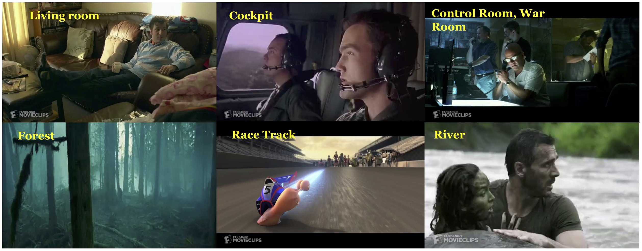
(a)

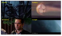
(b)

Figure 4: (a) Sample frames from the movie shots labeled by CLIP with high confidence (CLIPSceneScore $\geq$ 0.6 and Labels shown in yellow) (b) Sample frames from the movie shots tagged by CLIP with low confidence (Labels shown in yellow).

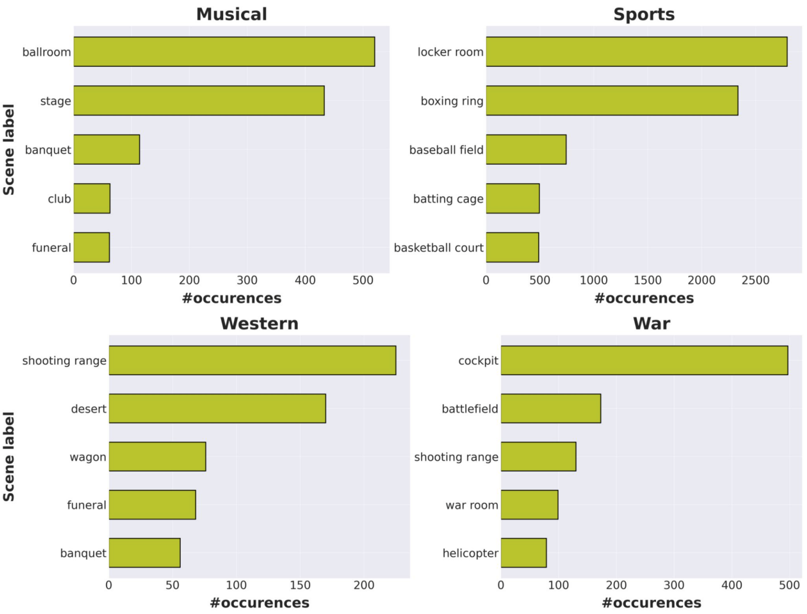
Figure 5: Genre wise distribution of different scene labels. For each genre, the top-5 scene labels are shown in terms of number of occurrences in the top-1 label provided by CLIP [41] for shots in MovieCLIP dataset. Threshold for confidence score of top-1 label = 0.4

Qualitative analysis: As shown in Fig 4a, CLIP performs well when distinctive elements of visual scene are present like background objects in indoor locations (living room) or appearance based cues (green color background for forests). For example in 4a, the presence of airplane windows indicate that the associated visual scene label with the given movie shot is cockpit. However, for shots involving blurry motion or absence of background information due to close up of the involved characters, CLIP’s confidence in associating visual scene labels is low (Fig 4b).
Genre-wise association: We consider those shots whose top-1 CLIPSceneScore values are greater than or equal to 0.4 and show the top-5 scene labels in terms of occurrences for certain genres like western, sport, war and musical. From Fig 5, we can see that relevant scenes are associated with genres through CLIP’s labeling scheme. Some notable examples include {shooting range, desert} for western, {locker room, boxing ring} for sport, {ballroom, stage} for musical and {cockpit, battlefield} for war.
Reliablity estimation: In order to estimate reliability of the top-k labels provided by CLIP for movie shots, we conduct a verification task on Amazon Mechanical Turk. We provided a pool of annotators with a subset of 2393 movie shots from VidSitu [46] dataset, along with top-5 scene labels. Out of the provided top-5 scene labels, the annotators were asked to select all the labels that apply for the given movie shot. We find 48.4% and 80% agreements among annotators in marking the top-1 and top-5 CLIP labels as relevant. After the human verification experiment is complete, we discard the shot samples with no agreements and obtain an evaluation data of 1883 shot samples.
Shot-type association: We consider the shots discarded in the reliability estimation phase to analyze distribution with various shot scale types. Based on the shot scale labels available as part of MovieShots dataset [42], we train a 2-layer LSTM (hidden dim= 512) [26] network using frame wise features from a pretrained ViT-B/16 [14] (extracted at 4 fps). The distribution of shot-wise predictions from the trained LSTM model is shown in Fig 6. We can see that 80% of shots having no agreements with human annotations belong to the shot categories having moderate (MS) to very high person closeup (ECS).

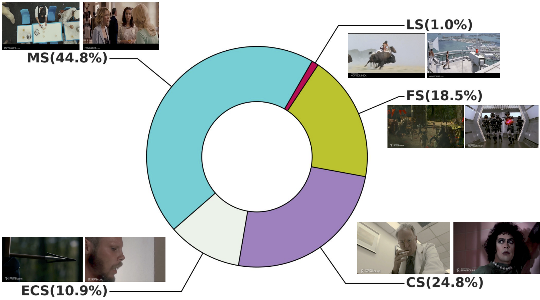
Figure 6: Distribution of shot scale predictions among the shots having no agreements between human annotators and CLIP’s labeling scheme. ECS: Extreme Close-up shot, CS: Close-up shot, MS: Medium shot, LS: Long shot, FS: Full shot

5 Experiments and Results

5.1 Experimental Setup

For training and validation purposes, we retain those shot samples whose top-1 CLIPSceneScore is greater than or equal to 0.4 (approx 75 percentile), resulting in a clean subset. After top-1 filtering, we also consider labels from top-k (k = 2 to 5) whose CLIPSceneScore is greater than 0.1 to associate multiple labels per sample. This results in a set of 107k samples with train, val and test split of 73.8k, 23.2k and 10.3k having non-intersecting set of ids with the human-verified evaluation set. Approximately 38.4% of the dataset is multi-label, covering 150 scene classes out of 179 in the curated scene taxonomy. All the related experiments were conducted using the Pytorch[39] framework using 4 T4 NVIDIA GPUs. For training the respective models, we use binary cross entropy loss function. For evaluation, we use mean average precision (mAP) and Pearson correlation (averaged across samples) as metrics.

5.2 Visual scene recognition - Movies

Frame wise aggregation models: For frame wise aggregation, we extract dense embeddings from individual shots at 4fps. We use two sets of embeddings: 512 dim embedding from Resnet18 [24] pretrained on Places2 dataset and 768 dim embedding from ViT-B/16 [14] model pretrained on Imagenet [11]. Following feature extraction, we perform temporal aggregation using LSTM [26] with 2 layers and hidden dimension of 512.
3D Convolutional network models: We use I3D[8], R(2+1)D [52], Slowfast [19] as baseline 3D convolutional models in multi-label setup. I3D[8] and Slowfast[19] models have a Resnet50[24] backbone whereas R(2+1)D [52] has a Resnet34[24] backbone. All the models are initialized from Kinetics400 [28] pretrained weights. For finetuning I3D[8] and Slowfast[19], we use SGD with learning rates in $\{0.1,1e-3\}$ and weight decay of 1e-4. For R(2+1)D [52] we use Adam [29] with learning rate 1e-4. Batch sizes for the models are varied between 16 and 32.
Video Transformer models: For video transformer models, we consider the base TimeSformer model [3] that considers 8 frames (224 x 224) as inputs. For finetuning TimeSformer [3] model, we use SGD with learning rate 5e-3 and weight decay of 1e-4 and batch size of 8. For better speed-accuracy tradeoff we use the Video Swin Transformer model [34], [33] called Swin-B with clip size of 32 frames (224 x 224) as inputs. For finetuning we use AdamW [35] optimizer with learning rate 1e-4 and Cosine Annealing with batch size of 32. More details of the hyperparameter settings for above mentioned models are included in Supplementary. Based on the results in Table 3, we can see that 2 layer LSTM models trained using features from Imagenet-21K pretrained ViT-B/16 perform better compared to features extracted using Resnet-18 model pretrained on Places2 dataset. This shows that features from Places2 pretrained models might not be optimal for scene recognition in the movie domain. In terms of end-to-end models, video transformers including TimeSformer and Swin-B models outperform 3D convolutional models. Swin-B model performs better than other models by obtaining an average correlation of 0.497 and mean average precision of 44.4.

Frame wise aggregation
Model	Features	mAP	Correlation
LSTM (512, 2 layers)	Places2 (4 fps)	24.15	0.29
LSTM (512, 2 layers)	ViT-B/16 (4 fps)	43.10	0.42
3D convolutional networks
Model	Features	mAP	Correlation
SlowFast (R50) [19]	NA	25.80	0.402
R(2+1)D (R34) [52]	NA	26.73	0.40
I3D (R50) [8]	NA	13.33	0.26
Video Transformers
TimeSformer [3]	NA	36.87	0.46
Swin-B [34]	NA	44.4	0.497

Table 3: Mean average precision (mAP) and average Spearman correlation of different models on human verified evaluation set (N=1883 shots). NA: End-to-end models used instead of features. For 3D conv models, the backbone network is mentioned inside brackets.

5.3 Downstream tasks

5.3.1 Visual scene recognition - web videos:

We also explore knowledge transfer from models finetuned on MovieCLIP by evaluating performance on downstream multi-label scene classification with HVU dataset [13]. For training and evaluation, we use 251k and 16k videos with 248 scene labels. We extract 1024 dim features from the best performing Swin-B model in Table 3. We train 3 layer fully connected models on the respective features with the following configuration:
$M_{scene}$: $\textbf{INP}[1024]\rightarrow{}\textbf{FC}[4096],\textbf{DO}(0.2)\rightarrow{}\textbf{FC}[4096]\\ \rightarrow{}\textbf{FC}[248]$
From Table 4, we can see that ${M_{scene}}$ exhibits better performance when compared to existing end-to-end models trained on HVU.

Model	mAP
3D-ResNet [13]	50.6
3D-STCNet [13]	51.9
HATNet [13]	55.8
${M_{scene}}$	55.92

Table 4: Mean average precision of different models on HVU dataset for multi label scene classification (248 classes). Backbone for end to end models: 3D Resnet18.

5.3.2 Multi label genre classification - Movie trailers:

Model	Overall	Ac	Ani	Bio	Com	Cri	Drm	Fmy	Fntsy	Hrrr	Myst	Rom	ScF	Thrl
$M_{trailer}$	56.14	62.97	86.51	14.4	80.77	49.58	79.58	74.55	49.59	50.62	26.83	45.05	47.99	61.36
C3D [51]	53.4	63.8	91.3	16.2	82.3	45.1	71.6	65.3	54.8	50.8	28.2	38.3	21.8	64.8
I3D [8]	38.8	37.2	51.8	9.2	72.6	33.9	67.6	43.6	39	22.8	21.3	34.3	22.6	48.3
LSTM [9]	48.4	47.5	86.8	12	79.2	33	72	64.5	54.4	22.7	24.7	40.4	36.5	54.8
Bi-LSTM [9]	47.4	49.9	86.3	8.2	77.6	29.9	70.8	65.4	55.3	22.3	21.7	41.6	35.9	51.2
fstVid [9]	56.5	61.4	94.8	23.9	81.5	41.7	77	67	62.6	36.1	30.4	48.4	48.2	62
fstTConv [9]	58.9	64.7	95.7	21.2	83.5	49.1	78.9	68.6	68.9	42.7	29.2	46.8	51	64.8

Table 5: Mean average precision of different models for multi-label genre classification (13 class) on Moviescope dataset. Except $M_{trailer}$ comparison results are reported from [9]. Abbreviations: Ac: Action, Ani: Animation, Bio: Biography, Com: Comedy, Cri: Crime, Drm: Drama, Fmy: Family, Fntsy: Fantasy, Hrrr: Horror, Myst: Mystery, Rom: Romantic, ScF: SciFi, Thrl: Thriller, fstVid: fastVideo, fstTConv: fastVideo + Temporal Conv.

As an additional downstream task, we consider multi-label genre classification of movie trailers in the Moviescope dataset [9]. Out of the original set of 4927 trailers, we could access 3900 videos from YouTube. Based on the provided splits, we use 2948, 410 and 542 videos for training, validation and testing purposes, respectively. We use the 1024 dim features extracted from the best performing Swin-B model in Table 3. We train 3 layer fully connected models on the respective features with the following configuration: $M_{trailer}$: $\textbf{INP}[1024]\rightarrow{}\textbf{FC}[512],\textbf{DO}(0.2)\rightarrow{}\textbf{FC}[512]\rightarrow{}\textbf{FC}[13]$
Even when the number of trailer videos used is a subset of the original split, $M_{trailer}$ exhibits similar genre wise trends as other models. From Table 5, we can see that $M_{trailer}$ shows better performance in Animation and Comedy as compared to genres like Biography and Mystery. When compared with fstTConv in Table 5, our fully connected model $M_{trailer}$ performs slightly worse due to non-availability of entire training data.

5.3.3 Impact of MovieCLIP pretraining:

HVU		Moviescope
Model	mAP	Model	mAP
$M_{scene}$	55.92	$M_{trailer}$	56.14
$M_{scene}(Kin)$	56.05	$M_{trailer}(Kin)$	53.29
Late Fusion	57.73	Late Fusion	56.29

Table 6: Impact of MovieCLIP pretrained features vs Kinetics pretrained features for $M_{scene}$ (HVU) and $M_{trailer}$ (Moviescope). Results reported are mean average precision (mAP) values. $Model(Kin)$: Model with Kinetics400 pretrained features, where $Model\in\{M_{scene},M_{trailer}\}$

.

We consider the impact of MovieCLIP based pretraining by fixing the fully connected architectures $M_{scene}$, $M_{trailer}$ and varying the input features. In the without MovieCLIP ($Kin$) pretraining setting, we extract 1024 dim features from Swin-B model pretrained on Kinetics400 for HVU and Moviescope datasets.

From Table 6, we can see that the performance of $M_{scene}$ with MovieCLIP pretrained features is comparable to $M_{scene}(Kin)$, even when the domain of Kinetics400 [28] is matched to HVU. Further, late fusion of prediction logits of $M_{scene}$ and $M_{scene}(Kin)$ with equal weights improves the mAP to 57.73 for HVU, thus indicating capture of complementary information, when trained with movie data. We include a class wise analysis of HVU dataset in Supplementary (Figure 11) to showcase the classes where MovieCLIP pretrained features improve upon Kinetics400 pretrained features. In case of Moviescope, $M_{trailer}$ results in improved performance (56.14) as compared to $M_{trailer}(Kin)$ (53.29), due to domain similarity with MovieCLIP dataset.

6 Ethical implications

Visual scene recognition capabilities can help in uncovering biases associated with the portrayal of under-represented and marginalized characters in various settings. For example, women are portrayed more in indoor scenes like kitchen, living room, hospital as compared to scenes like factory, laboratory or battlefield. Further, characters from marginalized demographic groups are often depicted in the background w.r.t common visual scenes, thus having considerable less share of speaking time. Apart from portrayal of characters, the usage of large scale pretrained models like CLIP [41] can help diagnose the inherent biases associated with its predictions since it is trained on free-form data curated from web. The proposed scheme of utilizing CLIP for weakly tagging datasets can reduce the costs associated with large-scale human expert driven annotation process.

7 Conclusion

In this work, we introduce a rich movie-centric taxonomy of visual scene labels, automatically curated from movie scripts and HVU [13], with minimal human-in-the loop intervention. Further, we utilize CLIP’s [41] zero-shot capabilities to weakly label movie shots based on our curated taxonomy in a scalable manner. We develop baseline end-to-end models on the weakly labelled dataset called MovieCLIP and evaluate on an independent human-verified dataset with scene labels. We explore the utility of MovieCLIP dataset as a pretraining source by evaluating on two downstream tasks of multi-label scene and genre classification of web videos [13] and movie trailers [9]. Future directions include modeling of temporal transitions of visual scenes across shots, multimodal association between audio events and visual scenes and multi-task modeling of visual scenes and related attributes like actions, time of day and settings (interior and exterior).

8 Acknowledgements

We would like to thank Boqing Gong for his feedback on the paper and help with experiment design. This work was supported by Google.

References

- [1] Max Bain, Arsha Nagrani, Andrew Brown, and Andrew Zisserman. Condensed movies: Story based retrieval with contextual embeddings, 2020.
- [2] Emad Barsoum, Cha Zhang, Cristian Canton Ferrer, and Zhengyou Zhang. Training deep networks for facial expression recognition with crowd-sourced label distribution. In ACM International Conference on Multimodal Interaction (ICMI), 2016.
- [3] Gedas Bertasius, Heng Wang, and Lorenzo Torresani. Is space-time attention all you need for video understanding? ArXiv, abs/2102.05095, 2021.
- [4] David Bordwell and Kirstin Thomson. Film art: An introduction. McGraw Hill, 2001, 2017.
- [5] Lukas Bossard, Matthieu Guillaumin, and Luc Van Gool. Food-101 -- mining discriminative components with random forests. In European Conference on Computer Vision, 2014.
- [6] Tom Brown, Benjamin Mann, Nick Ryder, Melanie Subbiah, Jared D Kaplan, Prafulla Dhariwal, Arvind Neelakantan, et al. Language models are few-shot learners. In Advances in Neural Information Processing Systems, volume 33, pages 1877--1901. Curran Associates, Inc., 2020.
- [7] João Carreira, Eric Noland, Chloe Hillier, and Andrew Zisserman. A short note on the kinetics-700 human action dataset. CoRR, abs/1907.06987, 2019.
- [8] J. Carreira and Andrew Zisserman. Quo vadis, action recognition? a new model and the kinetics dataset. pages 4724--4733, 07 2017.
- [9] Paola Cascante-Bonilla, Kalpathy Sitaraman, Mengjia Luo, and Vicente Ordonez. Moviescope: Large-scale analysis of movies using multiple modalities. ArXiv, abs/1908.03180, 2019.
- [10] Timothee Cour, Chris Jordan, Eleni Miltsakaki, and Ben Taskar. Movie/script: Alignment and parsing of video and text transcription. In David Forsyth, Philip Torr, and Andrew Zisserman, editors, Computer Vision -- ECCV 2008, pages 158--171, Berlin, Heidelberg, 2008. Springer Berlin Heidelberg.
- [11] Jia Deng, Wei Dong, Richard Socher, Li-Jia Li, Kai Li, and Li Fei-Fei. Imagenet: A large-scale hierarchical image database. In 2009 IEEE conference on computer vision and pattern recognition, pages 248--255. Ieee, 2009.
- [12] Karan Desai and Justin Johnson. VirTex: Learning Visual Representations from Textual Annotations. In CVPR, 2021.
- [13] Ali Diba, Mohsen Fayyaz, Vivek Sharma, Manohar Paluri, Jürgen Gall, Rainer Stiefelhagen, and Luc Van Gool. Large Scale Holistic Video Understanding. In Andrea Vedaldi, Horst Bischof, Thomas Brox, and Jan-Michael Frahm, editors, Computer Vision – ECCV 2020, pages 593--610, Cham, 2020. Springer International Publishing.
- [14] Alexey Dosovitskiy, Lucas Beyer, Alexander Kolesnikov, Dirk Weissenborn, Xiaohua Zhai, Thomas Unterthiner, Mostafa Dehghani, Matthias Minderer, Georg Heigold, Sylvain Gelly, Jakob Uszkoreit, and Neil Houlsby. An image is worth 16x16 words: Transformers for image recognition at scale. ICLR, 2021.
- [15] Mark Everingham, Josef Sivic, and Andrew Zisserman. Hello! my name is... buffy’’ -- automatic naming of characters in tv video. In BMVC, 2006.
- [16] Bernard Ghanem Fabian Caba Heilbron, Victor Escorcia and Juan Carlos Niebles. Activitynet: A large-scale video benchmark for human activity understanding. In Proceedings of the IEEE Conference on Computer Vision and Pattern Recognition, pages 961--970, 2015.
- [17] Li Fei-Fei, Rob Fergus, and Pietro Perona. Learning generative visual models from few training examples: An incremental bayesian approach tested on 101 object categories. Computer Vision and Pattern Recognition Workshop, 2004.
- [18] L. Fei-Fei and P. Perona. A bayesian hierarchical model for learning natural scene categories. In 2005 IEEE Computer Society Conference on Computer Vision and Pattern Recognition (CVPR’05), volume 2, pages 524--531 vol. 2, 2005.
- [19] Christoph Feichtenhofer, Haoqi Fan, Jitendra Malik, and Kaiming He. Slowfast networks for video recognition. In Proceedings of the IEEE international conference on computer vision, pages 6202--6211, 2019.
- [20] Brendan J. Frey and Delbert Dueck. Clustering by passing messages between data points. Science, 315(5814):972--976, 2007.
- [21] Raghav Goyal, Samira Ebrahimi Kahou, Vincent Michalski, Joanna Materzynska, Susanne Westphal, et al. The "something something" video database for learning and evaluating visual common sense. CoRR, abs/1706.04261, 2017.
- [22] Chunhui Gu, Chen Sun, David A Ross, Carl Vondrick, Caroline Pantofaru, et al. Ava: A video dataset of spatio-temporally localized atomic visual actions. In Proceedings of the IEEE Conference on Computer Vision and Pattern Recognition, pages 6047--6056, 2018.
- [23] Xiuye Gu, Tsung-Yi Lin, Weicheng Kuo, and Yin Cui. Open-vocabulary object detection via vision and language knowledge distillation. 2021.
- [24] Kaiming He, Xiangyu Zhang, Shaoqing Ren, and Jian Sun. Deep residual learning for image recognition. arXiv preprint arXiv:1512.03385, 2015.
- [25] Daniel Helm and Martin Kampel. Shot boundary detection for automatic video analysis of historical films. In Marco Cristani, Andrea Prati, Oswald Lanz, Stefano Messelodi, and Nicu Sebe, editors, New Trends in Image Analysis and Processing -- ICIAP 2019, pages 137--147, Cham, 2019. Springer International Publishing.
- [26] Sepp Hochreiter and Jürgen Schmidhuber. Long short-term memory. Neural computation, 9(8):1735--1780, 1997.
- [27] Qingqiu Huang, Yu Xiong, Anyi Rao, Jiaze Wang, and Dahua Lin. Movienet: A holistic dataset for movie understanding. In The European Conference on Computer Vision (ECCV), 2020.
- [28] Will Kay, João Carreira, Karen Simonyan, Brian Zhang, Chloe Hillier, Sudheendra Vijayanarasimhan, Fabio Viola, Tim Green, Trevor Back, Paul Natsev, Mustafa Suleyman, and Andrew Zisserman. The kinetics human action video dataset. CoRR, abs/1705.06950, 2017.
- [29] Diederik P. Kingma and Jimmy Ba. Adam: A method for stochastic optimization. CoRR, abs/1412.6980, 2015.
- [30] Jonathan Krause, Michael Stark, Jia Deng, and Li Fei-Fei. 3d object representations for fine-grained categorization. In 4th International IEEE Workshop on 3D Representation and Recognition (3dRR-13), Sydney, Australia, 2013.
- [31] Ivan Laptev, Marcin Marszalek, Cordelia Schmid, and Benjamin Rozenfeld. Learning realistic human actions from movies. In 2008 IEEE Conference on Computer Vision and Pattern Recognition, pages 1--8, 2008.
- [32] Boyi Li, Kilian Q. Weinberger, Serge J. Belongie, Vladlen Koltun, and René Ranftl. Language-driven semantic segmentation. ArXiv, abs/2201.03546, 2022.
- [33] Ze Liu, Yutong Lin, Yue Cao, Han Hu, Yixuan Wei, Zheng Zhang, Stephen Lin, and Baining Guo. Swin transformer: Hierarchical vision transformer using shifted windows. arXiv preprint arXiv:2103.14030, 2021.
- [34] Ze Liu, Jia Ning, Yue Cao, Yixuan Wei, Zheng Zhang, Stephen Lin, and Han Hu. Video swin transformer. arXiv preprint arXiv:2106.13230, 2021.
- [35] Ilya Loshchilov and Frank Hutter. Decoupled weight decay regularization. In ICLR, 2019.
- [36] Marcin Marszałek, Ivan Laptev, and Cordelia Schmid. Actions in context. In IEEE Conference on Computer Vision & Pattern Recognition, 2009.
- [37] José Gabriel Navarro. Film industry in the u.s. - statistics & facts. https://www.statista.com/topics/964/film/#dossierKeyfigures, 2021.
- [38] O. M. Parkhi, A. Vedaldi, A. Zisserman, and C. V. Jawahar. Cats and dogs. In IEEE Conference on Computer Vision and Pattern Recognition, 2012.
- [39] Adam Paszke, Sam Gross, Francisco Massa, Adam Lerer, James Bradbury, Gregory Chanan, Trevor Killeen, et al. Pytorch: An imperative style, high-performance deep learning library. In H. Wallach, H. Larochelle, A. Beygelzimer, F. d'Alché-Buc, E. Fox, and R. Garnett, editors, Advances in Neural Information Processing Systems 32, pages 8024--8035. Curran Associates, Inc., 2019.
- [40] Ariadna Quattoni and Antonio Torralba. Recognizing indoor scenes. In 2009 IEEE Conference on Computer Vision and Pattern Recognition, pages 413--420, 2009.
- [41] Alec Radford, Jong Wook Kim, Chris Hallacy, Aditya Ramesh, Gabriel Goh, et al. Learning transferable visual models from natural language supervision. CoRR, abs/2103.00020, 2021.
- [42] Anyi Rao, Jiaze Wang, Linning Xu, Xuekun Jiang, Qingqiu Huang, Bolei Zhou, and Dahua Lin. A unified framework for shot type classification based on subject centric lens. In The European Conference on Computer Vision (ECCV), 2020.
- [43] Jamie Ray, Heng Wang, Du Tran, Yufei Wang, Matt Feiszli, Lorenzo Torresani, and Manohar Paluri. Scenes-objects-actions: A multi-task, multi-label video dataset. In Computer Vision -- ECCV 2018, pages 660--676, Cham, 2018. Springer International Publishing.
- [44] Nils Reimers and Iryna Gurevych. Sentence-bert: Sentence embeddings using siamese bert-networks. In Proceedings of the 2019 Conference on Empirical Methods in Natural Language Processing. Association for Computational Linguistics, 11 2019.
- [45] Anna Rohrbach, Marcus Rohrbach, Niket Tandon, and Bernt Schiele. A dataset for movie description. 2015 IEEE Conference on Computer Vision and Pattern Recognition (CVPR), pages 3202--3212, 2015.
- [46] Arka Sadhu, Tanmay Gupta, Mark Yatskar, Ram Nevatia, and Aniruddha Kembhavi. Visual semantic role labeling for video understanding. In The IEEE Conference on Computer Vision and Pattern Recognition (CVPR), June 2021.
- [47] Mert Bulent Sariyildiz, Julien Perez, and Diane Larlus. Learning visual representations with caption annotations. In European Conference on Computer Vision (ECCV), 2020.
- [48] Sheng Shen, Liunian Harold Li, Hao Tan, Mohit Bansal, Anna Rohrbach, Kai-Wei Chang, Zhewei Yao, and Kurt Keutzer. How much can clip benefit vision-and-language tasks? ArXiv, abs/2107.06383, 2021.
- [49] Krishna Somandepalli, Tanaya Guha, Victor R. Martinez, Naveen Kumar, Hartwig Adam, and Shrikanth Narayanan. Computational media intelligence: Human-centered machine analysis of media. Proceedings of the IEEE, 109(5):891--910, 2021.
- [50] Khurram Soomro, Amir Roshan Zamir, and Mubarak Shah. UCF101: A dataset of 101 human actions classes from videos in the wild. CoRR, abs/1212.0402, 2012.
- [51] Du Tran, Lubomir Bourdev, Rob Fergus, Lorenzo Torresani, and Manohar Paluri. Learning spatiotemporal features with 3d convolutional networks. Dec. 2014.
- [52] Du Tran, Heng Wang, Lorenzo Torresani, Jamie Ray, Yann LeCun, and Manohar Paluri. A closer look at spatiotemporal convolutions for action recognition. In Proceedings of the IEEE conference on Computer Vision and Pattern Recognition, pages 6450--6459, 2018.
- [53] Ashish Vaswani, Noam Shazeer, Niki Parmar, et al. Attention is all you need. In I. Guyon, U. V. Luxburg, S. Bengio, H. Wallach, R. Fergus, S. Vishwanathan, and R. Garnett, editors, Advances in Neural Information Processing Systems, volume 30. Curran Associates, Inc., 2017.
- [54] Paul Vicol, Makarand Tapaswi, Lluis Castrejon, and Sanja Fidler. Moviegraphs: Towards understanding human-centric situations from videos. In IEEE Conference on Computer Vision and Pattern Recognition (CVPR), 2018.
- [55] Chao-Yuan Wu and Philipp Krähenbühl. Towards Long-Form Video Understanding. In CVPR, 2021.
- [56] Jianxiong Xiao, Krista A. Ehinger, James Hays, Antonio Torralba, and Aude Oliva. SUN Database: Exploring a Large Collection of Scene Categories. International Journal of Computer Vision, 119(1):3--22, Aug. 2016.
- [57] Bolei Zhou, Agata Lapedriza, Aditya Khosla, Aude Oliva, and Antonio Torralba. Places: A 10 million image database for scene recognition. IEEE Transactions on Pattern Analysis and Machine Intelligence, 2017.