Shepherding Heterogeneous Flock with Model-Based Discrimination

Abstract

The problem of guiding a flock of agents to a destination by the repulsion forces exerted by a smaller number of external agents is called the shepherding problem. This problem has attracted attention due to its potential applications, including diverting birds away for preventing airplane accidents, recovering spilled oil in the ocean, and guiding a swarm of robots for mapping. Although there have been various studies on the shepherding problem, most of them place the uniformity assumption on the dynamics of agents to be guided. However, we can find various practical situations where this assumption does not necessarily hold. In this paper, we propose a shepherding method for a flock of agents consisting of normal agents to be guided and other variant agents. In this method, the shepherd discriminates normal and variant agents based on their behaviors’ deviation from the one predicted by the potentially inaccurate model of the normal agents. As for the discrimination process, we propose two methods using static and dynamic thresholds. Our simulation results show that the proposed methods outperform a conventional method for various types of variant agents.

1 Introduction

The guidance and navigation of flocks of agents have several applications including guiding birds away from runways for preventing bird strikes [1], collecting oil spills in oceans and rivers [2, 3], and navigating a swarm of robots for map creation [4] and coverage [5]. For such systems, a variety of guidance methods for flocks have been proposed in the literature. The flock guidance methods available in the literature can be mainly classified into the following two categories: attraction-based guidance and repulsion-based guidance. Motivated by a recent comparison [6] of these two types of guidance methods suggesting the potential superiority of the repulsion-based method over the attraction-based method, this paper focuses on the repulsion-based guidance of flocks of agents.

The repulsion-based guidance framework for flocks called shepherding [7] is an emergent framework inspired by the behavior of sheepdogs guiding a flock of sheep. Specifically, the shepherding problem refers to the problem of designing the movement law of a small number of external steering agents (called shepherds) so that they can guide, with their repulsion force, a larger number of agents (called sheep) to a given destination. Consequently, in the course of the navigation by the shepherd agents, the sheep agents move according to their inter-flock interactions and the repulsive forces from the shepherds. As for the inter-flock interactions, the following three types of interactions in the Boid model [8] are often assumed: separation, alignment, and attraction.

In the literature of the shepherding problem, we can find several movement laws of shepherds for guiding the sheep agents under various problem settings. For example, Vaghan et al. [9] proposed a shepherd’s movement law in which the shepherd agent accomplishes guidance by moving toward the center of the sheep flock, and demonstrated the law’s effectiveness through robotic experiments for guiding a flock of ducks. Strömbom et al. [10] proposed a shepherd’s movement law in which the shepherd alternatively uses the following two different methods inspired by the behavior of actual sheepdogs: collecting, which brings closer to the flock the individuals away from the flock, and driving, which brings the whole flock to the goal. Tsunoda et al. [11] proposed a shepherd’s movement law, called the Farthest-Agent Targeting (FAT) method, in which the shepherd guides the sheep farthest from the destination, and have shown that the proposed movement law can outperofrm the movement laws of Vaghan et al. and Strömbom et al. The same authors have further shown in their another work [12] an improved version of the FAT method by introducing a modification for preventing the scatterment of flocks. Hu et al. [13] proposed a shepherding method in which the shepherd guides the flock by going behind the herd, and showed the effectiveness of the method by both simulations and robotic experiments. Ko and Zuazua [14] proposed a feedback-based shepherding method for a flock of agents trying to escape from a goal area.

A common practice in the literature of the shepherding problem is placing the uniformity assumption on the dynamics within the flock of sheep agents to be guided. However, this assumption does not necessarily hold true in several practical scenarios. For example, while fish form schools to protect themselves from predators, the dynamics of each individual is not necessarily uniform [15]. On the other hand, in the context of the swarm robotics, heterogeneity within the swarm can be found due to fluctuations in production processes [16, 17] or by the intent of the operator of the swarm [18]. In order to address the aforementioned gap between the literature and the practice, Himo et al. [19] recently proposed a guidance method for a flock containing agents not responding to the shepherd agent. Although this work sheds light on the shepherding-type guidance of a heterogeneous flock, the guidance method still assumes the shepherd’s knowledge of the type of each sheep agent, thereby having a limited applicability in some practical situations. For example, in emergency crowd control situations, people may engage in unexpected behaviors such as pushing and trampling. However, it is difficult to know in advance who will behave unexpectedly because these behaviors are based on individual instincts, experiences, and the actions of those around them (see, e.g., [20, 21]).

Therefore, in this paper, we consider a problem of shepherding a heterogeneous flock with a shepherd agent having no prior information on the type of each sheep. We specifically consider a situation in which a flock consists of the following two types of sheep agents: normal sheep agents and variant sheep agents. As for the normal sheep agents, the shepherd is assumed to be given information about their dynamics. On the other hand, as for the variant sheep agents, we assume that their dynamics are different from those of the normal sheep and, furthermore, are unknown to the shepherd. A major difference of our problem formulation from the one in [19] is that we allow the dynamics of the variant sheep to lack any of the alignment, separation, attraction, and repulsion from the shepherd. Therefore, the situation we consider in this paper includes the case in which the navigation of the variant sheep is essentially a difficult task. For this reason, in our problem formulation, we consider the navigation of only the normal sheep. Hence, the goal of the guidance by the shepherd is set to be guiding the group of only the normal agents to the destination area.

Because we assume that the shepherd has no prior knowledge on the type of respective sheep, the methodology presented in [19] is not directly applicable to the current problem setting. Therefore, in this paper, we propose a discrimination method in which the nominal model of the normal sheep agents is utilized. Specifically, the shepherd internally predicts the trajectory of sheep agents under the assumption that all the sheep are normal. The shepherd then computes the deviation of the trajectory of each sheep from its prediction for discriminating agents. Finally, for agents that are not discriminated to be variant, the shepherd agent applies the FAT method to guide them to the destination area. We remark that, due to this model-based characteristics of the discrimination process, the proposed shepherding method can be considered to be an application of the framework called Model Predictive Control (MPC) in the systems and control theory [22]. Although there exist several works on the Model Predictive Control of heterogeneous multi-agent systems (see, e.g., [23, 24]), their direct application to the current problem is not necessarily realistic due to the high nonlinearity in the Boid model. For this reason, in this paper we develop a novel shepherding algorithm and, furthermore, aim to establish its effectiveness via extensive numerial simulations.

This paper is organized as follows. In Section 2, we formulate the shepherding problem studied in this paper. In Section 3, we describe the proposed guidance method based on model-based discrimination. In Section 4, we evaluate the effectiveness of the proposed method through comparison with the FAT method by numerical simulations. We specifically evaluate the dependence of the guidance success rate on the type and the number of variant agents. In Section 5, we conclude the paper and discuss future research directions.

2 Problem statement

In this section, we formulate the shepherding problem studied in this paper. Let us consider a multi-agent system on the two-dimensional plane $\mathbb{R}^{2}$. The multi-agent system consists of $N$ agents, each of which is either to be guided or not to be guided, and one steering agent performing navigation. Following the convention in the literature [7], we call the agents to be guided as sheep, and the steering agent as a shepherd. As shall be described in Subsection 2.1, the sheep agents move on the plane according to the inter-flock dynamics and the repulsive force from the shepherd agent. The objective of the shepherd agent is set to be the guidance of the sheep agents to be guided into a goal region $G$, which is assumed to be an open disk with center $x_{g}\in\mathbb{R}^{2}$ and radius $R_{g}>0$.

Throughout this paper, we use the following notations. We assign the numbers $1$, …, $N$ to the sheep agents. The set of these numbers is denoted as $[N]=\{1,\dotsc,N\}$. Also, we let $x_{d}(k)\in\mathbb{R}^{2}$ denote the position of the shepherd agent at time $k$, and $x_{i}(k)\in\mathbb{R}^{2}$ denote the position of the $i$th sheep at time $k$. For a set $X$, we let $\lvert X\rvert$ denote the number of elements of $X$. For a real vector $v$, we let $\lVert v\rVert$ denote the Euclidean norm of $v$.

2.1 Sheep dynamics

In this subsection, we present the mathematical model of the movement of sheep agents. We assume that, at each time $k$, the position $x_{i}(k)$ of the $i$th sheep is updated by the difference equation

$$x_{i}(k+1)=x_{i}(k)+v_{i}(k),$$ (1)

where $v_{i}(k)\in\mathbb{R}^{2}$ denotes the movement vector of the $i$th sheep at time $k$. In this paper, we assume that the vector $v_{i}(k)$ is constructed according to the Boid model [8], a model widely used in the context of the shepherding problem [25, 10, 11, 26, 27] In the Boid model, the following three types of inter-flock interactions are assumed: “separative force” from other agents, “alignment force” to match the speed of other agents, and “attractive force” to approach other agents. In addition to these three types of interactions, the sheep are assumed to move in such a way as to avoid the shepherd. Then, the vector $v_{i}(k)$ appearing in equation (1) is determined as

$$v_{i}(k)=K_{i1}v_{i1}(k)+{K_{i2}v_{i2}(k)}+K_{i3}v_{i3}(k)+K_{i4}v_{i4}(k),$$ (2)

where $K_{i1}$, $K_{i2}$, $K_{i3}$, and $K_{i4}$ are non-negative constants that depend on individual sheep. Also, $v_{i1}(k)$, $v_{i2}(k)$, and $v_{i3}(k)$ are vectors corresponding to the separative, alignment, and attractive forces of the Boid model, respectively. To these three vectors we add vector $v_{i4}(k)$ corresponding to the repulsive force from the shepherd.

We assume that the $i$th sheep receives forces from all sheep in the circle with center $x_{i}(k)$ and radius $R>0$. If there are no other sheep in this range, then we set $v_{i1}(k)=v_{i2}(k)=v_{i3}(k)=0$. If we let $S_{i}(k)$ denote the set of the indices of the sheep within radius $R$ of the $i$th sheep at time $k$, then the vectors $v_{i1}(k)$, $v_{i2}(k)$, and $v_{i3}(k)$ are given by

$$v_{i1}(k) =-\frac{1}{|S_{i}(k)|}\sum_{j\in S_{i}(k)}\frac{x_{j}(k)-x_{i}(k)}{\lVert x_{j}(k)-x_{i}(k)\rVert^{3}},$$ (3)

$$v_{i2}(k) =\frac{1}{|S_{i}(k)|}\sum_{j\in S_{i}(k)}\frac{v_{j}(k-1)}{\lVert v_{j}(k-1)\rVert},$$ (4)

$$v_{i3}(k) =\frac{1}{|S_{i}(k)|}\sum_{j\in S_{i}(k)}\frac{x_{j}(k)-x_{i}(k)}{\lVert x_{j}(k)-x_{i}(k)\rVert},$$ (5)

whereas $v_{i4}(k)$ is given by

$$v_{i4}(k) =-\frac{x_{d}(k)-x_{i}(k)}{\lVert x_{d}(k)-x_{i}(k)\rVert^{3}}.$$ (6)

2.2 Guidance problem

In the shepherding problem we consider in this paper, it is supposed that the sheep agents consists of the following two types of sheep; normal and variant. A normal sheep is assumed to be subject to all the four types of forces (3)–(6): separation, alignment, attraction, and repulsion from the shepherd. On the other hand, a variant sheep is assumed to be subject to at most three types of the four forces. Therefore, we do not consider the situation in which a variant sheep receives all the four forces but with different coefficients. We place this assumption for simplicity of the formulation; in particular, the shepherding method developed in this paper is applicable to such general cases.

We assume that there exist $M$ variant sheep. Without loss of generality, we assume that the sheep $1$, $2$, …, $N-M$ are normal, and the sheep $N-M+1$, $N-M+2$, …, $N$ are variant. In this paper, we do not consider heterogeneity within the set of the normal sheep and the one of the variant sheep. Hence, we assume the existence of positive constants $K_{1}$, $K_{2}$, $K_{3}$, and $K_{4}$ such that

$$K_{i1}=K_{1},\ K_{i2}=K_{2},\ K_{i3}=K_{3},\ K_{i4}=K_{4}$$ (7)

for all $i=1,\dotsc,N-M$. Likewise, we assume the existence of nonnegative constants $\alpha_{1}$, $\alpha_{2}$, $\alpha_{3}$, and $\alpha_{4}$ such that

$$K_{i1}=\alpha_{1}K_{1},\ K_{i2}=\alpha_{2}K_{2},\ K_{i3}=\alpha_{3}K_{3},\ K_{i4}=\alpha_{4}K_{4}$$ (8)

for all $i=N-M+1,\dotsc,N$. We remark that the quadruple

$$\alpha=(\alpha_{1},\alpha_{2},\alpha_{3},\alpha_{4})$$ (9)

characterizes the deviation of the dynamics of the variant sheep from that of the normal sheep. In this paper, we suppose that each coefficient $\alpha_{i}$ is either $0$ or $1$. Under this assumption, for example, if a variant sheep receives only the forces of separation and alignment, then we have $\alpha=(1,1,0,0)$.

As for the information available to the shepherd, we consider the following situation. First, we assume that the shepherd is initially given an estimate

$$(\beta_{1}K_{1},\beta_{2}K_{2},\beta_{3}K_{3},\beta_{4}K_{4})$$ (10)

of the coefficients $(K_{1},K_{2},K_{3},K_{4})$ characterizing the dynamics of the normal sheep. We do not require that the estimate is correct; therefore, each of the constants $\beta_{1}$, $\beta_{2}$, $\beta_{3}$, and $\beta_{4}$ is not necessarily equal to one. Secondly we assume that, in the process of the guidance operation, the shepherd will be given the location of all the sheep at every $T$ units of time from an external system for observation; i.e., we assume that the shepherd can obtain the set of vectors

$$\{x_{i}(\ell T)\}_{i\in[N]}$$ (11)

for each $\ell\geq 0$. Finally, in addition to this global but periodic information, we suppose that the shepherd is able to measure the position of the sheep closest to the shepherd at every time instants to avoid collision. Hence, the shepherd is assumed to know the index

$$n(k)=\operatorname*{argmin}_{i\in[N]}{\lVert x_{d}(k)-x_{i}(k)\rVert}.$$ (12)

at each time $k\geq 0$.

We can now state the objective of this paper as follows.

Problem 2.1.

Develop a movement algorithm of the shepherd so that the shepherd can let as many normal sheep as possible arrive into the destination area $G$ by using the information (10), (11), (12) given to the shepherd.

3 Proposed method

In this section, we describe the proposed shepherding method based on model-based discrimination of variant sheep agents. In Subsection 3.1, we describe the overall behavior of the proposed method. Then, in Subsection 3.2, we introduce auxiliary agents called virtual sheep, which play an important role in the proposed method. A detailed description of the proposed method is presented in Subsection 3.3.

3.1 Overall behavior

Let us first describe the overall behavior of the proposed method. We first remark that, in the special case where a variant sheep does not exist, that is, when all the sheep are normal, then applying the FAT method [12] can be considered to be effective to solve Problem 2.1. However, as shown by the authors in [19], existence of a variant sheep would prevent the successful guidance by the FAT method. One possibility in this context is applying the FAT method only to the flock of normal sheep in all sheep. However, in this paper, we are assuming that the shepherd is not given the labels (i.e., normal or variant) of sheep. In order to overcome this limitation, in this paper we propose that the shepherd performs discrimination of sheep agents by using their degree of deviation from their predicted trajectory. The details of the prediction method is presented in Subsection 3.2, and that of the discrimination method is presented in Subsection 3.3.

For prediction of the sheep’s trajectory, the proposed method uses the coefficients $(\beta_{1}K_{1},\beta_{2}K_{2},\beta_{3}K_{3},\beta_{4}K_{4})$ given to the shepherd as an estimate of the coefficient characterizing the normal sheep. If the estimate is accurate, i.e., if the estimate $(\beta_{1}K_{1},\beta_{2}K_{2},\beta_{3}K_{3},\beta_{4}K_{4})$ is closer to the normal coefficients $(K_{1},K_{2},K_{3},K_{4})$ than to the variant coefficients $(\alpha_{1}K_{1},\alpha_{2}K_{2},\alpha_{3}K_{3},\alpha_{4}K_{4})$, then we can expect that the trajectory prediction for normal sheep is more accurate than that for variant sheep. Based on this supposition, the proposed method determines that sheep with larger prediction errors are variant and, then, excludes them from the shepherd’s navigation. Specifically, the shepherd uses the FAT method to guide only those sheep not discriminated to be variant.

3.2 Dynamics of virtual sheep

In this subsection, we formally introduce the agents called virtual sheep, which we use to perform the trajectory prediction of the actual sheep. These agents are assumed to be placed one for each of the actual sheep agents. These $N$ virtual sheep move on the field $\mathbb{R}^{2}$ in a way similar to that of the actual sheep, baesd on the estimated coefficients $(\beta_{1}K_{1},\beta_{2}K_{2},\beta_{3}K_{3},\beta_{4}K_{4})$ given to the shepherd.

Let the position of the $i$th virtual sheep at time $k$ be denoted by $\xi_{i}(k)$. Then, the change in position of the virtual sheep is specified as

$$\xi_{i}(k+1)=\begin{cases}\displaystyle x_{i}(k),&\mbox{if $k\bmod T=0$},\\ \xi_{i}(k)+\phi_{i}(k),&\mbox{otherwise.}\end{cases}$$ (13)

In this equation, we assume that the position of the $i$th virtual sheep is re-positioned to the same position as the (actual) $i$th sheep at every $T$ units of time, when a global measurement (11) of the sheep positions become available to the shepherd. This re-positioning allows us to prevent an unlimited growth of the distance between the normal and the virtual sheep caused by their difference in dynamics, which is therefore necessary for performing discrimination effectively. Furthermore, $\phi_{i}(k)$ is the vector representing the movement of the virtual sheep at time $k$, and is determined in a way similar to equation (2) for the actual sheep as

$$\phi_{i}(k)=\beta_{1}K_{1}\phi_{i1}(k)+\beta_{2}K_{2}\phi_{i2}(k)+\beta_{3}K_{3}\phi_{i3}(k)+\beta_{4}K_{4}\phi_{i4}(k),$$ (14)

where $\beta_{1}K_{1}$, $\beta_{2}K_{2}$, $\beta_{3}K_{3}$, and $\beta_{4}K_{4}$ are the estimated coefficients of the normal sheep and are given in advance to the shepherd. Also, $\phi_{i1}(k)$, $\phi_{i2}(k)$, $\phi_{i3}(k)$, and $\phi_{i4}(k)$ are vectors corresponding to separation, alignment, attraction, and repulsion from the shepherd, respectively. Because the global measurement (11) is available only periodically, between two consecutive global measurements, the virtual sheep is assumed to perform its motion with reference to the virtual sheep’s position and displacement. Therefore, the vectors in the equation (14) are constructed as

$$\phi_{i1}(k) =-\frac{1}{|T_{i}(k)|}\sum_{j\in T_{i}(k)}\frac{\xi_{j}(k)-\xi_{i}(k)}{\|\xi_{j}(k)-\xi_{i}(k)\|^{3}},$$ (15)

$$\phi_{i2}(k) =\frac{1}{|T_{i}(k)|}\sum_{j\in T_{i}(k)}\frac{\phi_{j}(k-1)}{\|\phi_{j}(k-1)\|},$$ (16)

$$\phi_{i3}(k) =\frac{1}{|T_{i}(k)|}\sum_{j\in T_{i}(k)}\frac{\xi_{j}(k)-\xi_{i}(k)}{\|\xi_{j}(k)-\xi_{i}(k)\|},$$ (17)

$$\phi_{i4}(k) =-\frac{x_{d}(k)-\xi_{i}(k)}{\|x_{d}(k)-\xi_{i}(k)\|^{3}},$$ (18)

where $T_{i}(k)\subset[N]$ is the set of indices of the virtual sheep within radius $R$ of the $i$th virtual sheep at time $k$, and is defined by

$$T_{i}(k)=\{j\in[N]\backslash\{i\}\mid\lVert\xi_{j}(k)-\xi_{i}(k)\rVert\leq R\}.$$ (19)

If $T_{i}(k)$ equals the empty set, then we set $\phi_{i1}(k)=\phi_{i2}(k)=\phi_{i3}(k)=0$.

3.3 Movement algorithm of shepherd

We are now ready to describe the proposed movement algorithm of the shepherd. The proposed method is based on the FAT method. In the original FAT method [12], a sheep called the target sheep is selected from among all the sheep. On the other hand, the proposed method selects sheep only from those discriminated to be normal by the shepherd. The discrimination is performed by using the virtual sheep introduced in Subsection 3.2.

In the algorithm, the shepherd possesses as its internal variable a set $I(k)\subset[N]$, which is used to record the set of the sheep index discriminated to be normal. The shepherd first initializes this set as $I(0)=[N]$ and update the set with period $T$. At each time instant for update, a sheep index that is discriminated to be variant is removed from the set. The discrimination is performed by the rule described later in this subsection. On the other hand, for all the sheep that have been once removed from the set $I(k)$, the shepherd checks a condition described below. If the sheep satisfies the condition, then its corresponding index is recovered into the set.

For discrimination, with period $T$, the shepherd computes the distance $\lVert x_{i}(k)-\xi_{i}(k)\rVert$ between the actual and virtual sheep for all $i\in[N]$. If this distance is greater than a threshold value $L$, then the $i$th sheep is discriminated to be variant and, therefore, is removed from the set $I(k)$. As for determining the threshold, we propose the following two methods; Static and Dynamic. The Static method uses a fixed threshold, while the Dynamic method dynamically and adaptatively sets the threshold using quartile ranges, a common outlier detection method in statistics. Specifically, in the latter approach, the first quartile $q_{1}$ and third quartile $q_{3}$ are first computed for the set $\{\lVert x_{i}(k)-\xi_{i}(k)\rVert\}_{i\in[N]}$ of the distances. Then, the distance threshold $L$ is determined as

$$L=q_{3}+1.5\;\mathrm{IQR}$$ (20)

with the interquartile range $\mathrm{IQR}=q_{3}-q_{1}$.

At each update time of the set $I(k)$, once the shepherd finishes discrimination of all the sheep agents, the shepherd then adds the index $i$ to the set $I(k)$ for all sheep $i\notin I(k)$ that have been determined to be variant, if the number of times the sheep has been determined to be variant is less than the pre-determined threshold $\tau>0$ and, furthermore, $h$ units of time has passed since its last discrimination to be variant. Thus, for a sheep to be permanently removed from the set $I(k)$, the sheep must be determined to be variant $\tau+1$ times. The reason for introducing this mechanism is that the above decision method is not always accurate due to the potential error in the coefficient estimate given to the shepherd. Even when the estimate is correct, the non-vanishing distance between a variant sheep and its corresponding virtual sheep causes the difference in the trajectories of a normal sheep and its corresponding virtual sheep, particularly when the normal sheep has relatively many variant neighbors. With the intention of compensating for this imprecision, we set the threshold $\tau$ in the proposed decision algorithm.

For the set $I(k)$ thus constructed, the shepherd performs guidance based on the FAT method proposed in [12] as follows. First, we let the shepherd change its position from time $k$ to $k+1$ as

$$x_{d}(k+1)=x_{d}(k)+v_{d}(k),$$ (21)

where $v_{d}(k)$ is the vector of shepherd movements at time $k$ and is constructed as

$$v_{d}(k)=K_{d_{1}}v_{1}(k)+K_{d_{2}}v_{2}(k)+K_{d_{3}}v_{3}(k).$$ (22)

In this equation, $K_{d_{1}}$, $K_{d_{2}}$, and $K_{d_{3}}$ are positive constants, and the vectors $v_{1}(k)$, $v_{2}(k)$, and $v_{3}(k)$ are given by

$$v_{1}(k) =\frac{x_{d}(k)-x_{t(k)}(k)}{\|x_{d}(k)-x_{t(k)}(k)\|},$$ (23)

$$v_{2}(k) =-\frac{x_{d}(k)-x_{n(k)}(k)}{\|x_{d}(k)-x_{n(k)}(k)\|^{3}},$$ (24)

$$v_{3}(k) =-\frac{x_{d}(k)-x_{g}}{\|x_{d}(k)-x_{g}\|},$$ (25)

where $t(k)$ denotes the estimated index of the sheep farthest from the goal among those discriminated to be normal, and is constructed as

$$t(k)=\begin{cases}\operatorname*{argmax}_{i\in I(k)}{\lVert x_{i}(k)-x_{g}\rVert},&\mbox{if $k\bmod T=0$},\\ t(k-1),&\mbox{otherwise,}\end{cases}$$ (26)

while $n(k)$ is the index of the sheep closest to the shepherd and is defined as in (12). We remark that, in the original FAT method, the shepherd is designed to steer the sheep farthest from the goal among all the sheep agents. However, since we assume that the shepherd can observe the actual positions of all the sheep only periodically, we alternatively adopt the formula (26) as the estimate of the normal sheep farthest from the goal.

Finally, the proposed method terminates when all the sheep in the set $I(k)$ are in the destination area $G$. A flowchart of the entire algorithm presented in this section is shown in Figure 1.

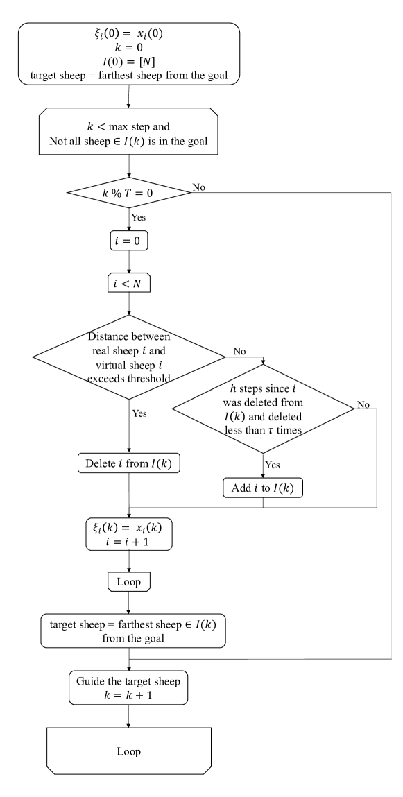
Figure 1: Flowchart of the proposed shepherding method

4 Numerical simulations

The objective of this section is to demonstrate the effectiveness of the proposed method through numerical simulations. As the performance measure for the comparison of shepherding methods, we adopt the guidance success rate, which is defined as the number of the normal sheep that could be guided to the destination area at the end of executing the algorithms. In Subsection 4.1, we first describe the setup of our simulations. We then, in Subsection 4.2, present our comparison of the proposed method with the FAT method and, furthermore, the comparison among the proposed methods (i.e., Static and Dynamic).

4.1 Simulation setting

Coefficients of normal sheep dynamics (2) Notation Description Value $K_{1}$ Separation $100$ $K_{2}$ Alignment $0.5$ $K_{3}$ Attraction $2$ $K_{4}$ Repulsion $500$ $R$ Radius of recognition range $20$ Coefficients of shepherd dynamics (22) Notation Description Value $K_{d_{1}}$ Attraction to $t(k)$th sheep $10$ $K_{d_{2}}$ Separation from $n(k)$th sheep $200$ $K_{d_{3}}$ Repulsion from goal $4$

Throughout our numerical simulations, the coefficients in the dynamic model of the normal sheep (equations (2) and (7)) and those of the shepherd (22) are set as in Tables 4.1 and 4.1, respectively. These values of the coefficients are the same as the ones used in [19]. We set the total number $N$ of the sheep to be $20$, and the maximum simulation step to be $10000$ throughout all simulations. We assumed that, at the initial time $t=0$, each sheep is randomly placed according to a uniform distribution on the open disk with center at the origin and radius $60$. The initial position of the shepherd is set to be $(-30,-50)$. On the other hand, as for the destination area, we set its center $x_{g}$ to be $(20,20)$ and its radius to be $15$. We set the period $T$ at which a shepherd can observe the position of arbitrary sheep to $10$. We have also set the time interval $h$ for re-including a sheep once discriminated to be variant into the set $I(k)$ to be $20$, and the threshold $\tau$ for permanently removing a sheep from the target of guidance to be $5$. Finally, we set the distance threshold in the Static method as $L=5$.

As for the coefficients $\beta_{1}$, $\beta_{2}$, $\beta_{3}$, and $\beta_{4}$ appearing in the estimates (10) given to the shepherd, we set $\beta_{i}=1$ for the forces received by the variant sheep, and set $\beta_{i}=0.9$ for the forces not received by a variant sheep. For example, when a variant sheep is subject to only separative and attractive forces, i.e., if $\alpha=(1,0,1,0)$, then we set $\beta=(1,0.9,1,0.9)$. In our simulations, we consider the variance types characterized by the vectors $(\alpha_{1},\alpha_{2},\alpha_{3},\alpha_{4})$ ($\alpha_{i}\in\{0,1\}$, $i=1,2,3,4$) except for the trivial cases of $(1,1,1,1)$ and $(0,0,0,0)$. Hence, there are the total of $14$ types of variant sheep considered in our simulations.

Using the settings described above, we randomly generated 100 initial arrangements of sheep and, then, performed simulations. We define the guidance success rate as the average number of normal sheep that could be guided to the destination at the end of the algorithm in these $100$ simulations.

4.2 Simulatoin results

In this subsection, we perform comparison of the proposed methods and FAT method, as well as the comparison among the proposed methods. Specifically, in Subsection 4.2.1, we compare the performance of the proposed and conventional methods by observing the dependency of their guidance success rate on the number of variant sheep. Then, in Subsection 4.2.2, we compare the two proposed methods thorough the evaluation of their frequency of misjudgement, i.e., the number of times at which a normal sheep is erroneously discriminated as variant.

4.2.1 Comparison of the proposed and conventional methods

We first demonstrate the overall behaviors of the proposed and conventional methods. In this demonstration, we use the Static method as the proposed algorithm, and also assume that the variant sheep receives only the force of separation (i.e., $\alpha=(1,0,0,0)$). We show the timeline of the guidance by the FAT method and the proposed method in Figure 2. In Figure 2a, we illustrate a typical situation in which the FAT method fails to guide the whole flock because the shepherd keeps trying to guide a variant sheep. On the other hand, as we can see from Figure 2b, the proposed method enables the shepherd to discriminate normal and variant sheep and to guide the normal sheep successfully in the goal region.

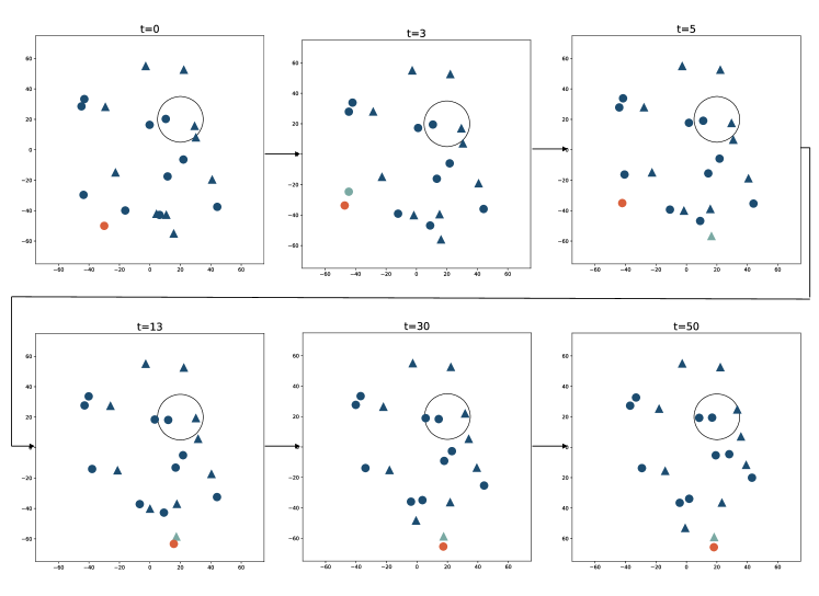
(a) FAT method. The guidance fails because the sheepdog keep trying to guide a variant sheep.

(b) Static method. The shepherd guide only normal sheep by not guiding the variant sheep.

Figure 2: Timeline of the guidance by the FAT and the Static method. The red circle indicate the sheepdog, the circles indicate normal sheep, and the triangles indicate variant sheep receive only the force of separation. The light blue represents the target sheep at the time.

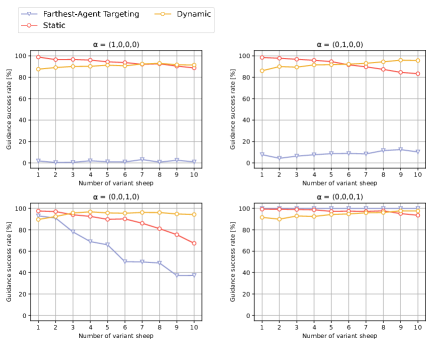
(a) The variant sheep receive one force.

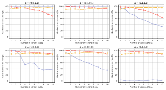
(b) The variant sheep receive two forces.

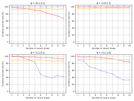
(c) The variant sheep receive three forces.

Figure 3: Guidance success rate by FAT method and two proposed shepherding methods. The blue, red, and orange lines indicate the induction rate by FAT, Static, and Virtual, respectively.

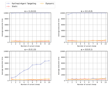
(a) The variant sheep receive one force.

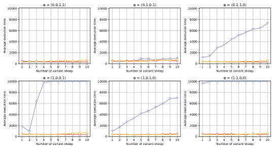
(b) The variant sheep receive two forces.

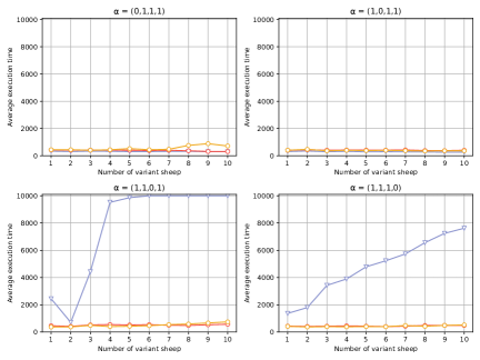
(c) The variant sheep receive three forces.

Figure 4: Average execution time by FAT method and two proposed shepherding methods. The blue, red, and orange lines indicate the average execution time by FAT, Static, and Virtual, respectively.

Let us then compare the performances of the proposed methods and the FAT method. In Figure 3, we show the guidance success rates by the proposed methods (Static and Dynamic) and the FAT method for various values of $M$ (i.e., the number of the variant sheep). The FAT method achieves 100% guidance success rate for the cases of 1) the variant sheep receives repulsion but not separation ($\alpha=(0,1,1,1),\ (0,0,1,1),\ (0,1,0,1),\ (0,0,0,1)$) and 2) receives all forces but alignment ($\alpha=(1,0,1,1)$). However, for the flock containing variant sheep that receive neither attraction nor repulsion (i.e., when $\alpha=(1,1,0,0),\ (1,0,0,0),\ (0,1,0,0)$), the FAT method frequently fails to guide the flock (guidance success rate $<13\%$). Furthermore, for the case of other types of variant sheep, the FAT method shows the trend in which the guidance success rate decreases with respect to the number of the variant sheep in the flock. On the other hand, we can observe that both of the proposed methods exhibits relatively high performance (guidance success rates $>63\%$) irrespective of the type of variant sheep, confirming their effectiveness and robustness.

In order to further investigate the difference in the performances of the proposed and the FAT methods, we compare the average execution time (i.e., the average number of steps taken by the algorithms). We show the average execution times of the algorithms in Figure 4. We can confirm that the proposed methods finish guidance relatively quickly (average execution time $<530$). On the other hand, the FAT method requires much longer execution time. This is mainly because the termination criterion of the FAT method is that all the sheep lie in the goal region, which does not often happen when the flock of the sheep contains variant ones.

4.2.2 Comparison of Static and Dynamic methods

In this subsection, we further investigate and discuss the difference in the performance of the two proposed methods (Static and Dynamic). From Figure 3, we find that the guidance success rate of the Static method tends to decrease with respect to the number $M$ of variant sheep. The reason for this characteristic can be attributed to the fact that, the more the variant sheep, the more deviated the trajectories of the virtual sheep to those of the normal sheep. This quantitative change cannot necessarily be appropriately dealt with by the fixed threshold of the Static method. On the other hand, the guidance success rate by the Dynamic method does not exhibit such trend and, furthermore, even increases with respect to $M$ for some types of variant sheep. A possible reason for this phenomenon is that, in the Dynamic method, when there are few variant sheep, its threshold would become relatively small because the difference of the overall dynamics of the flock of virtual sheep and that of actual sheep is small. This would let the threshold of the Dynamic method relatively small, which then can make it difficult for the shepherd to discriminate variant sheep. Similarly, when there are relatively many variant sheep, the Dynamic method would make its threshold high, which then would prevent the shepherd from misjudging a normal sheep as a variant sheep. These two factors can explain the trend in Figure 3 in which the Dynamic method does not perform as better as the Static method for a small $M$, but can outperform the Static method for larger $M$.

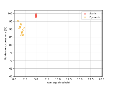
(a) $M=1$

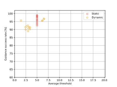
(b) $M=4$

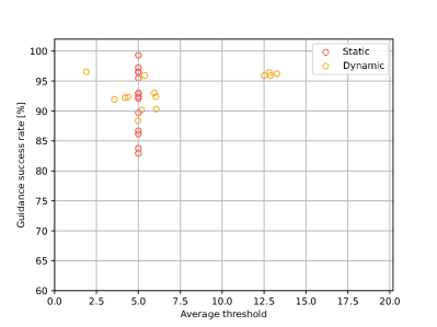
(c) $M=7$

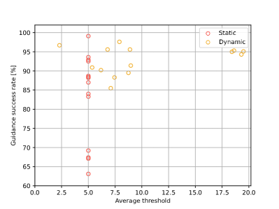
(d) $M=10$

Figure 5: Relationship between the thresholds and guidance success rate. Horizontal axis: The value of the thresholds. Vertical axis: Guidance success rate.

In order to further investigate the relationship between the guidance success rate and the thresholds, let us investigate how the guidance success rate depends on the value of the threshold. We show their relationship in Figure 5. In the figure, each plot consists of $14\times 2=28$ points resulting form all the pairs of the type of the variant sheep and the two threshold method. Therefore, each point represents the average of the threshold and the guidance success rate from the corresponding 100 simulations. The points from the static method lies on the same vertical line because the method uses a fixed threshold $5$. On the other hand, because the Dynamic method adaptatively changes its threshold in the course of the shepherding guidance, the points do not necessarily lie on the same vertical line.

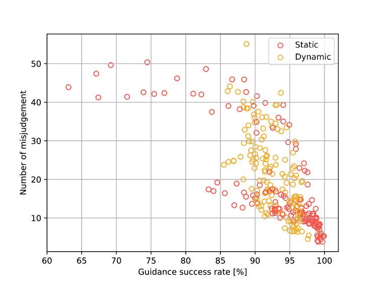
Figure 6: Relationship between guidance success rate and the number of incorrect discrimination of the normal sheep. Horizontal axis: Guidance success rate. Vertical axis: The number of times a normal sheep is mistakenly judged to be a variant one.

From Figure 5, we reconfirm that increasing $M$ can result in degradation of the performance of the Static method. On the other hand, we observe that the average threshold in the Dynamic method tends to increase with $M$, while the guidance success rate is mostly maintained for all the types of the variant sheep. This trend would be because varying the size of the threshold enabled the Dynamic method to reduce the number of times a normal sheep is mistakenly judged to be variant. These observations suggest that preventing a wrong discrimination of a normal sheep would lead to better guidance success rate.

In order to assess the validity of our hypothesis that preventing discrimination of a normal sheep as a variant sheep would lead to increase in the guidance success rate, let us examine how the guidance success rate depends on the occurrence of the incorrect discrimination. In Figure 6, we show the relationship between the guidance success rate and the number of incorrect discrimination of the normal sheep. The overall negative correlation from the plot, both in the Static and Dynamic method, confirms the validity of our hypothesis.

5 Conclusion

In this paper, we have formulated a shepherding problem for a heterogeneous flock consisting of normal and variant sheep, and then proposed a movement algorithm of the shepherd to solve the formulated shepherding problem. In this algorithm, the shepherd predicts the sheep’s trajectories using the given and estimated dynamical model of normal sheep. Then, the shepherd discriminates those sheep deviating from the predicted trajectory as variant. To the agents discriminated to be normal, the shepherd performs navigation control by using the FAT algorithm. We specifically proposed two methods having a different discrimination process; Static, in which the distance threshold for discrimination is constant, and Dynamic, in which the threshold adaptatively changes. Our numerical simulations show that both methods outperform the FAT method in its original form. We also find that the Dynamic method is robust to the change in the number of the variant sheep in the flock of agents.

There are several interesting directions of future research. One is a further comprehensive investigation of the performance of the proposed method. For example, in this paper, we have focused on the situation in which the uniformity among the variant sheep is guaranteed. Investigating how the heterogeneity within the variant sheep affects the performance of the proposed methods is necessary to further establish their effectiveness. Another direction is to validate the effectiveness of the proposed discrimination method when used in the shepherding methods other than the FAT method.

References

- [1] Gade S, Paranjape AA, Chung SJ. Herding a flock of birds approaching an airport using an unmanned aerial vehicle. In: AIAA Guidance, Navigation, and Control Conference; 2015. p. 1540.
- [2] Zahugi EMH, Shanta MM, Prasad T. Oil spill cleaning up using swarm of robots. In: Advances in computing and information technology. Springer; 2013. p. 215–224.
- [3] Pashna M, Yusof R, Ismail ZH, Namerikawa T, et al. Autonomous multi-robot tracking system for oil spills on sea surface based on hybrid fuzzy distribution and potential field approach. Ocean Engineering. 2020;207:107238.
- [4] Kegeleirs M, Grisetti G, Birattari M. Swarm slam: Challenges and perspectives. Frontiers in Robotics and AI. 2021;8:23.
- [5] Gusrialdi A, Hirche S, Hatanaka T, Fujita M, et al. Voronoi based coverage control with anisotropic sensors. In: 2008 American Control Conference; 2008. p. 736–741.
- [6] Goel R, Lewis J, Goodrich MA, Sujit PB. Leader and predator based swarm steering for multiple tasks. In: 2019 IEEE International Conference on Systems, Man and Cybernetics; 2019. p. 3791–3798.
- [7] Long NK, Sammut K, Sgarioto D, Garratt M, et al. A comprehensive review of shepherding as a bio-inspired swarm-robotics guidance approach. IEEE Transactions on Emerging Topics in Computational Intelligence. 2020;4(4):523–537.
- [8] Reynolds CW. Flocks, herds and schools: A distributed behavioral model. In: 14th Annual Conference on Computer Graphics and Interactive Techniques; 1987. p. 25–34.
- [9] Vaughan R, Sumpter N, Frost A, Cameron S. Robot sheepdog project achieves automatic flock control. In: Fifth International Conference on the Simulation of Adaptive Behaviour; Vol. 489; 1998. p. 493.
- [10] Strömbom D, Mann RP, Wilson AM, Hailes S, et al. Solving the shepherding problem: heuristics for herding autonomous, interacting agents. Journal of the Royal Society Interface. 2014;11(100).
- [11] Tsunoda Y, Sueoka Y, Sato Y, Osuka K. Analysis of local-camera-based shepherding navigation. Advanced Robotics. 2018;32(23):1217–1228.
- [12] Tsunoda Y, Ishitani M, Sueoka Y, Osuka K. Analysis of sheepdog-type navigation for a sheep model with dynamics. In: 24th International Symposium on Artificial Life and Robotics 2019; 2019. p. 499–503.
- [13] Hu J, Turgut AE, Krajník T, et al. Occlusion-based coordination protocol design for autonomous robotic shepherding tasks. IEEE Transactions on Cognitive and Developmental Systems. 2020;.
- [14] Ko D, Zuazua E. Asymptotic behavior and control of a “guidance by repulsion” model. Mathematical Models and Methods in Applied Sciences. 2020;30(04):765–804.
- [15] Hemelrijk CK, Hildenbrandt H. Self-organized shape and frontal density of fish schools. Ethology. 2008;114(3):245–254.
- [16] Sakurama K. Clique-Based distributed PI control for multiagent coordination with heterogeneous, uncertain, time-varying orientations. IEEE Transactions on Control of Network Systems. 2020;7(4):1712–1722.
- [17] Sakurama K, Nakano K. Necessary and sufficient condition for average consensus of networked multi-agent systems with heterogeneous time delays. International Journal of Systems Science. 2015;46(5):818–830.
- [18] Aotani T, Kobayashi T, Sugimoto K. Bottom-up multi-agent reinforcement learning for selective cooperation. In: 2018 IEEE International Conference on Systems, Man, and Cybernetics; 2018. p. 3590–3595.
- [19] Himo R, Ogura M, Wakamiya N. Iterative algorithm for shepherding unresponsive sheep. Mathematical Biosciences and Engineering. 2022;19(4):3509–3525.
- [20] Pan X, Han CS, Dauber K, et al. A multi-agent based framework for the simulation of human and social behaviors during emergency evacuations. Ai & Society. 2007;22(2):113–132.
- [21] Fujita A, Feliciani C, Yanagisawa D, et al. Traffic flow in a crowd of pedestrians walking at different speeds. Physical Review E. 2019;99(6):062307.
- [22] Mayne DQ. Model predictive control: Recent developments and future promise. Automatica. 2014;50(12):2967–2986.
- [23] Okajima T, Tsumura K, Hayakawa T, et al. Leader following of partially heterogeneous multi-agent systems via cooperative adaptive control. In: 21st International Symposium on Mathematical Theory of Networks and Systems; 2014. p. 1582–1588.
- [24] Kawamura S, Cai K, Kishida M. Robust output regulation of networked heterogeneous linear agents by distributed internal model principle. In: 58th IEEE Conference on Decision and Control; 2019. p. 7301–7306.
- [25] Fujioka K. Effective Herding in Shepherding Problem in V-formation Control. Transactions of the Institute of Systems, Control and Information Engineers. 2018;31(1):21–27.
- [26] El-Fiqi H, Campbell B, Elsayed S, et al. The limits of reactive shepherding approaches for swarm guidance. IEEE Access. 2020;8:214658–214671.
- [27] Zhi J, Lien JM. Learning to herd agents amongst obstacles: training robust shepherding behaviors using deep reinforcement learning. IEEE Robotics and Automation Letters. 2021;6(2):4163–4168.