Entire Space Counterfactual Learning: Tuning, Analytical Properties and Industrial Applications

Abstract

As a basic research problem for building effective recommender system, post-click conversion rate (CVR) estimation has long been plagued by data sparsity and sample selection bias issues. To mitigate the data sparsity issue, prevalent methods based on entire space multitask model construct auxiliary learning tasks by harnessing the sequential track of user behaviors, i.e., exposure $\rightarrow$ click $\rightarrow$ conversion. However, they still fall short of the two primary defects: (1) intrinsic estimation bias (IEB), where the CVR estimates are intrinsically greater than the actual values; (2) false independence prior (FIP), where the causation from click to post-click conversion might be overlooked. On this basis, this paper further proposes a model-agnostic method named entire space counterfactual multi-task model (ESCM²) that utilizes a counterfactual risk minimizer to handle both IEB and FIP issues at once. To demonstrate the superiority of ESCM², this paper explores its parameter tuning in practice, derives its analytic properties, and showcases its effectiveness in industry, where ESCM² can effectively alleviate the intrinsic IEB and FIP issues and outperform baseline models.

I Introduction

Recommendation system seeks to deliver valuable items to users to meet their interest [1, 2, 3], driving user growth in e-commerce [4], advertising [5], and social media [6]. Fig. 1 depicts a typical content-based recommendation pipeline in industry, which consists of the offline and online phases. In the offline phase, item attributes, user profiles, and their interactions are extracted from logs to train a multitask ranking model. In the online phase, the ranking model ranks all candidate items according to the estimated click-through rate (CTR), post-click conversion rate (CVR), and click-through&conversion rate (CTCVR). On this basis, items are exposed to users to meet with their personalized preferences. Finally, the performance of the ranking model would be optimized based on real-time user feedback.

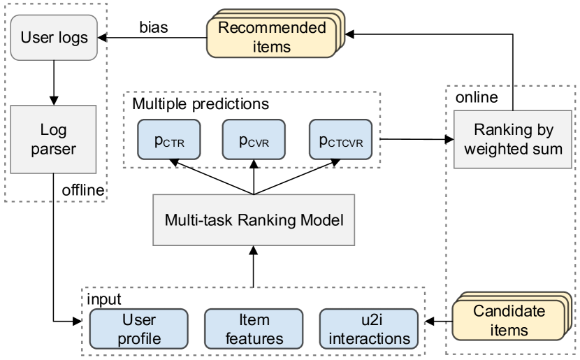
Figure 1: Overview of a two-stage recommender in industry.

One typical track of user behavior [4] in industry can be expressed as exposure $\to$ click $\to$ conversion in Fig. 2. In this context, CTR represents the transition chance from exposure space to click space; CVR represents that from click space to conversion space; and CTCVR represents that from exposure space to conversion space. The growth of large-scale database and feature interaction approaches has made CTR estimation a well-established practice and revenue source in the industry [7, 8, 9]. However, click-through feedback frequently misrepresents the actual user preferences since it is easily tainted by many factors in practice, e.g., clickbait [10, 11]. In contrast, post-click feedback, i.e., CVR, faithfully reflects user preferences and directly influences gross merchandise volume, attracting special attention in recommendation committee.

A naïve but widely selected approach [12] to constructing CVR estimators is training the estimator over the click space $\mathcal{O}$, in which conversion labels are completely observable. However, there are two key problems with this strategy. The first issue is sample selection bias i.e., the training space only consists of user-item intersections where click takes place, whereas the inference space is the entire exposure space $\mathcal{D}$. Since the intersections with lower CVR are more likely to be excluded from the training space $\mathcal{O}$ [13, 14], training data is missing not at random [12], which leads to a bias between the training space and inference space. The second issue is the sparsity of clicked samples [4, 14]. With a CTR of 4% for the Ali-CPP benchmark and 3.8% for our industrial benchmark, the amount of training data is extremely insufficient to develop a generalizable CVR estimator. In summary, both of these issues significantly hinder the generalization and online performance of the naïve approach beyond the click space.

Figure 2: Overview of CVR estimation task in recommendation, where online inference is conducted on all exposed samples, but training is only performed on clicked samples, yielding data sparsity and sample selection bias.

The entire space multitask model (ESMM) [4] is an intuitive approach to mitigate both issues by avoiding direct training of CVR estimators. The key insight is to break down the CVR estimation task into CTR and CTCVR estimation that can be trained over the exposure space. It effectively mitigates data sparsity, and yields substantial gains in industry [15, 16]. However, the unbiasedness of its CVR estimation remains not ensured, which raises serious concerns. In this study, we mainly investigate two limitations of ESMM as follows:

• Intrinsic Estimation Bias (IEB), where the CVR estimates are intrinsically biased against the actual values.

• False Independence Prior (FIP), where the CTR and CVR estimates are susceptible to conditional independence, which is undesirable since the causal dependency from click to conversion is falsely overlooked.

Inspired by causality paradigm, a model-agnostic approach named Entire Space Counterfactual Multitask Model (ESCM²) is proposed, which incorporates a counterfactual risk minimizer to regularize the CVR estimator in the ESMM framework. As discussed in Section IV, the analytical properties of the proposed regularizer successfully handle both IEB and FIP defects. The contributions of this study are threefold:

• We demonstrate that ESMM’s CVR estimates suffer from the intrinsic estimation bias, providing experimental results and mathematical analysis to support this claim.

• We demonstrate that ESMM introduces false independence prior to its CTCVR estimates, with well crafted experiments to support this claim.

• We develop ESCM², which is the first effort to suggest a causal improvement to ESMM. With ESCM², the IEB and FIP issues in ESMM are effectively handled. We back up our assertions with a plethora of real-world experiments and mathematical analysis.

This paper is an extension of our work [17] presented in SIGIR’22. Based on this prior work we have made extensions in several aspects. First, we have presented relevant theorems and proofs to demonstrate that the proposed doubly robust estimator handles IEB and FIP concerns. Then, the proposed regularizers’ statistical properties (i.e., bias and variance) have been investigated for rigor. Moreover, we have demonstrated that ESCM² is a particular Monte Carlo’s approach, which could motivate a large number of theoretical extensions. Finally, we have added details of model structure, online A/B test and emerging related works.

The remaining sections are structured as follows: Section II provides some preliminaries to better understand the proposed method. Section III investigates the IEB and FIP issues with ESMM. We introduce the proposed counterfactual regularizers in Section IV-A, analyze their theoretical effectiveness to handle the IEB and FIP issues in Section IV-B, and summarize the implementation of ESCM² in Section IV-C. To demonstrate the superiority of ESCM², real-word case studies are conducted in Section V. Section VI is an overview of related works; Section VII discusses conclusions and open questions.

II Preliminaries

II-A Notations

In this paper, uppercase letters, e.g., $O$, represent random variables; lowercase letters, e.g., $o$, represent the associated specific values; calligraphic letters such as $\mathcal{O}$ denote sample spaces; $\mathbb{P}(\cdot)$, $\mathbb{E}(\cdot)$, $\mathbb{V}(\cdot)$ represent probability distribution, expectation and variance, respectively.

II-B Problem Statement

Denote $\mathcal{U}=\{u_{1},u_{2},...,u_{m}\}$ and $\mathcal{I}=\{i_{1},i_{2},...,i_{n}\}$ as the set of users and items over exposure space, respectively. Let $\mathcal{D}=\mathcal{U}\times\mathcal{I}$ be the set of user-item intersections in the exposure space. Let $\mathbf{O}\in\{0,1\}^{m\times n}$ be the click indicators where $o_{u,i}\in\{0,1\}$ indicates whether the user $u$ clicks the item $i$; $\mathbf{R}\in\{0,1\}^{m\times n}$ be the conversion labels where $r_{u,i}\in\{0,1\}$ indicates whether the user $u$ purchases the item $i$.

If all entries $r_{u,i}\in\mathbf{R}$ are observable, the ideal learning objective for constructing CVR estimator is expressed as

$$\mathcal{P}:=\mathbb{E}_{(u,i)\in\mathcal{D}}\left[\delta\left(r_{u,i},\hat{r}_{u,i}\right)\right],$$ (1)

where $\hat{r}_{u,i}$ denotes the estimate of $r_{u,i}$, $\delta$ measures the estimation error and can be implemented with any classification loss function. Following existing works [14, 4], the binary cross-entropy is employed in this study as the loss measure:

$$\delta(r_{u,i},\hat{r}_{u,i}):=-r_{u,i}\log\hat{r}_{u,i}-(1-r_{u,i})\log(1-\hat{r}_{u,i}).$$ (2)

However, $r_{u,i}$ is non-observable for user-item intersections outside the click space $\mathcal{O}$, rendering (1) incomputable. Therefore, it is a common practice to estimate the learning objective with user-item intersections in $\mathcal{O}$:

$$\mathcal{L}_{\mathrm{naive}}:=\mathbb{E}_{(u,i)\in\mathcal{O}}(\delta_{u,i})=\frac{1}{|\mathcal{O}|}\sum_{(u,i)\in\mathcal{D}}(o_{u,i}\delta_{u,i}),$$ (3)

where $|\mathcal{O}|=\sum_{(u,i)\in\mathcal{D}}(o_{u,i})$, $\delta_{u,i}$ is short for $\delta(r_{u,i},\hat{r}_{u,i})$. Nonetheless, (3) yields biased CVR estimation [12, 18], i.e., $\mathbb{E}_{O}[\mathcal{L}_{\mathrm{naive}}]\neq\mathcal{P}$, which hinders its application in the industry.

II-C Entire Space Multitask Model Approach

ESMM [4] exploits the sequential user behavior track in Fig. 2 to estimate CVR indirectly. It decomposes CVR as

$$\mathbb{P}(r_{u,i}=1\mid o_{u,i}=1)=\frac{\mathbb{P}(r_{u,i}=1,o_{u,i}=1)}{\mathbb{P}(o_{u,i}=1)}.$$ (4)

Then, it constructs two towers to model CTR and CVR as $\mathbb{P}(o_{u,i}=1)$ and $\mathbb{P}(r_{u,i}=1\mid o_{u,i}=1)$, respectively; and estimates CTCVR as $\mathbb{P}(r_{u,i}=1,o_{u,i}=1)$ by multiplying the outputs of these two towers. In the training phase, the learning objective is to minimize the empirical risk of CTR and CTCVR estimates in $\mathcal{D}$ where feedback is fully observed:

$$\mathcal{L}_{\mathrm{CTR}} :=\mathbb{E}_{(u,i)\in\mathcal{D}}\left[\delta\left(o_{u,i},\hat{o}_{u,i}\right)\right]$$ (5)

$$\mathcal{L}_{\mathrm{CTCVR}} :=\mathbb{E}_{(u,i)\in\mathcal{D}}\left[\delta\left(o_{u,i}*r_{u,i},\hat{o}_{u,i}*\hat{r}_{u,i}\right)\right].$$

In the inference phase, the output of the CVR tower serves as its CVR estimate. This approach circumvents the selection bias via optimizing CVR estimator in an implicit way; however, as shown in Section III-A, it is still susceptible to the intrinsic bias. To properly handle the sample selection bias of CVR estimation, an unbiased CVR estimator is required.

II-D Causal Recommendation Approach

Recently, the recommendation community has placed special attention on causal inference techniques. We concentrate on those based on propensity scores because they are prevalent in estimating CVR. In the context of CVR estimation, the propensity score given a particular user-item intersection is equivalent to its click-through rate:

$$q_{u,i}:=\mathbb{P}(O=1\mid u,i).$$ (6)

To handle sample selection bias, the inverse propensity score (IPS) [12] approach balances the distributions of error terms ${\delta_{u,i}}:=\delta(r_{u,i},\hat{r}(u,i))$ between the training and inference space by re-weighting. Specifically, based on (6), it inversely weights each error term with the propensity score:

$$\mathcal{L}_{\mathrm{IPS}}:=\mathbb{E}_{(u,i)\in\mathcal{D}}\left[\frac{o_{u,i}\delta_{u,i}}{q_{u,i}}\right].$$ (7)

Since the actual $q_{u,i}$ is unavailable, it is common to estimate it using CTR estimate $\hat{o}_{u,i}$ [12]. Notably, (7) is an unbiased estimator of the ideal learning objective in (1), i.e., $\mathbb{E}_{O}(\mathcal{L}_{\mathrm{IPS}})=\mathcal{P}$, given accurate CTR estimate, i.e., $\hat{o}_{u,i}=q_{u,i}$.

Nonetheless, this method suffers from severe high variance as the CTR estimates are frequently close to zero. The doubly robust (DR) estimator [18] further mitigates this high variance via error imputation technique [19]. Specifically, it first constructs an imputation model $\hat{\delta}_{u,i}$ to impute the CVR estimation error in $\mathcal{D}$, and corrects the imputation with $\hat{e}_{u,i}=\delta_{u,i}-\hat{\delta}_{u,i}$ in $\mathcal{O}$. The learning objective can be formulated as

$$\mathcal{L}_{\mathrm{DR}}:=\mathbb{E}_{(u,i)\in\mathcal{D}}\left[\hat{\delta}_{u,i}+\frac{o_{u,i}\hat{e}_{u,i}}{q_{u,i}}\right],$$ (8)

where $q_{u,i}$ eliminates the MNAR effect for $\hat{e}_{u,i}$. As long as either the imputed error $\hat{\delta}_{u,i}$ or the CTR estimate $\hat{o}_{u,i}$ is accurate, (8) is unbiased, leading to double robustness. The accuracy of $\hat{\delta}_{u,i}$ and $\hat{q}_{u,i}$ is ensured by auxiliary tasks.

III Analysis of Entire Space Multitask Model

In this section, two primary issues of ESMM are investigated: (1) intrinsic estimation bias, where the CVR estimates are always higher against the actual values; (2) false independence prior, where the causation from click to conversion is not explicitly modeled, making the CTR and CVR estimates susceptible to independence in prior.

III-A Intrinsic Estimation Bias

The effect of ESMM’s bias for CVR estimation has been empirically observed in practice [14]. Nonetheless, a formal justification and theoretical analysis remains lacking. To this end, we formulate the intrinsic estimation bias in Proposition 1, and demonstrate its existence under proper assumptions.

Proposition 1.

Denote click, post-click conversion and click & conversion as random variables $O,R,C$; let $o_{u,i},r_{u,i},c_{u,i}$ be the associated values given user-item intersections; $\hat{o}_{u,i},\hat{r}_{u,i},\hat{c}_{u,i}$ be the estimated values of $o_{u,i},r_{u,i},c_{u,i}$. ESMM overestimates the CVR expectation over exposure space $\mathcal{D}$:

$$\mathrm{Bias}^{\mathrm{ESMM}}:=\mathbb{E}_{\mathcal{D}}\left[\hat{R}\right]-\mathbb{E}_{\mathcal{D}}\left[R\right]>0,$$ (9)

under the mild assumption that conversion is more likely to take place for user-item intersections over click space [12]:

$$\mathbb{E}_{\mathcal{O}}\left[R\right]>\mathbb{E}_{\mathcal{D}}\left[R\right].$$ (10)

Proof.

According to the learning objectives in (5), one properly trained ESMM guarantees:

$$\mathbb{E}_{\mathcal{D}}\left[O-\hat{O}\right] =\int\left(o_{u,i}-\hat{o}_{u,i}\right)\mathop{d}\!d(u,i)=0$$ (11)

$$\mathbb{E}_{\mathcal{D}}\left[C-\hat{C}\right] =\int\left(c_{u,i}-\hat{c}_{u,i}\right)\mathop{d}\!d(u,i)=0.$$

Recall that $\mathbb{E}_{\mathcal{D}}\left[R\right]$ and $\mathbb{E}_{\mathcal{D}}\left[\hat{R}\right]$ are the expected values of the true CVR and its estimates, respectively. The bias of CVR estimate can be expressed as

$$\mathrm{Bias}^{\mathrm{ESMM}} =\mathbb{E}_{\mathcal{D}}\left[\hat{R}\right]-\mathbb{E}_{\mathcal{D}}\left[R\right]$$

$$>\mathbb{E}_{\mathcal{D}}\left[\hat{R}\right]-\mathbb{E}_{\mathcal{O}}\left[R\right]$$ (12a)

$$=\mathbb{E}_{\mathcal{D}}\left[\hat{R}\right]-\frac{\mathbb{E}_{\mathcal{D}}\left[C\right]}{\mathbb{E}_{\mathcal{D}}\left[O\right]}$$ (12b)

$$=\mathbb{E}_{\mathcal{D}}\left[\frac{\hat{C}}{\hat{O}}\right]-\frac{\mathbb{E}_{\mathcal{D}}\left[C\right]}{\mathbb{E}_{\mathcal{D}}\left[O\right]},$$ (12c)

where (12a) exploits the assumption in (10); (12b) decomposes the expectation of actual CVR over $\mathcal{O}$ using the user behavior track in Fig. 2, (12c) follows the decomposition in (4).

In exposure space, denote the joint probability of $\hat{C}=\hat{c}$ and $\hat{O}=\hat{o}$ as $\mathbb{P}(\hat{c},\hat{o})$. The first term in (12c) can be rewritten as

$$\mathbb{E}_{\mathcal{D}}\left[\frac{\hat{C}}{\hat{O}}\right] =\int\frac{\hat{c}}{\hat{o}}\mathbb{P}(\hat{c},\hat{o})d(\hat{c},\hat{o})$$ (13a)

$$=\int\frac{\hat{c}}{\hat{o}}\mathbb{P}(\hat{c})\mathbb{P}(\hat{o})d(\hat{c},\hat{o})$$ (13b)

$$=\int\hat{c}\mathbb{P}(\hat{c})d\hat{c}\int\frac{1}{\hat{o}}\mathbb{P}(\hat{o})d\hat{o}$$ (13c)

$$=\mathbb{E}_{\mathcal{D}}\left[\hat{C}\right]\mathbb{E}_{\mathcal{D}}\left[\frac{1}{\hat{O}}\right]$$ (13d)

$$\geq\frac{\mathbb{E}_{\mathcal{D}}\left[\hat{C}\right]}{\mathbb{E}_{\mathcal{D}}\left[\hat{O}\right]}$$ (13e)

$$=\frac{\mathbb{E}_{\mathcal{D}}\left[C\right]}{\mathbb{E}_{\mathcal{D}}\left[O\right]}.$$ (13f)

Below is step-by-step derivation:

• (13a) expands the expectation of $\hat{C}/\hat{O}$;

• (13b) holds under a stringent assumption $\hat{O}\upmodels\hat{C}$;

• (13c) decomposes the integrals and prompts (13d);

• (13e) exploits the Jensen inequality $\mathbb{E}\left[f(X)\right]\geq f\left(\mathbb{E}\left[X\right]\right)$ for convex function $f(X)=1/X$; where the equality holds only when the variance of $X$ is zero;

• (13f) is ensured by a properly trained ESMM in (11).

As a result, ESMM’s CVR estimates are always higher than the actual values, i.e., $\mathrm{Bias}^{\mathrm{ESMM}}>0$. The proof is completed. ∎

Proposition 1 formulates and demonstrates the IEB problem with ESMM’s CVR estimate. This drives us to suggest an unbiased CVR estimator and explicitly handle the IEB problem, as opposed to circumventing this crucial issue by employing a multitask modeling technique over the entire space.

III-B False Independence Prior

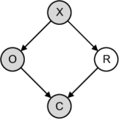
(a) ESMM Method

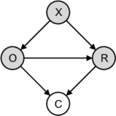
(b) Naïve Method

(c) ESCM² Method

Figure 3: Causal graphs where X, R, O, C denote the user-item intersection, conversion, click and click & conversion, respectively. Hollow and shaded nodes indicate latent and observed variables, respectively. The blue circle in (c) represents intervention, blocking the backdoor path X $\rightarrow$ O.

To estimate CTCVR, two towers are developed in ESMM to estimate CTR and CVR, and the product of their outputs are used to estimate CTCVR:

$$\mathbb{P}(o_{u,i}=1,r_{u,i}=1)=\mathbb{P}(o_{u,i}=1)*\mathbb{P}(r_{u,i}=1\mid o_{u,i}=1),$$ (14)

where the CVR estimate is click-dependent, i.e., conversion only occurs after the click, yielding a causal link O $\rightarrow$ R in the physical data generation process. However, ESMM’s learning objective (5) fails to portray this causal dependency explicitly, indicated by the missing arrow O $\rightarrow$ R in Fig. 3 (a). It poses the risk that ESMM models CVR as $\mathbb{P}(r_{u,i}=1)$ following Fig. 3 (a), as opposed to the expected $\mathbb{P}(r_{u,i}=1\mid o_{u,i}=1)$ in (14). This risk is formulated as false independence prior, as it confuses the expected $\mathbb{P}(r_{u,i}=1\mid o_{u,i}=1)$ in (14) and unexpected $\mathbb{P}(r_{u,i}=1)$, thus introducing false independent prior in CTCVR estimation.

The naïve approach [14] in (3) trains the CVR model within the click space, thus explicitly incorporating the dependency O $\rightarrow$ R as depicted in Fig. 3 (b). However, the back-door path X $\rightarrow$ O leads to sample selection bias [4, 14]. Through a causal lens, the key to solving FIP without introducing a backdoor path is formulating CVR as a causal estimand:

$$\mathbb{P}(r_{u,i}=1\mid\textit{do}(o_{u,i}=1)),$$ (15)

where ”do” represents the do-calculus [22], truncating the backdoor path X $\rightarrow$ O as shown in Fig. 3. For the clicked samples, (15) is consistent with the standard definition of CVR, but for the unclicked samples, it turns to modeling the counterfactual problem: ”How likely is a user to be converted if she clicks the item?”. On this basis, CTCVR is refined as

$$\mathbb{P}\left(o_{u,i}=1,r_{u,i}=1\right)=\mathbb{P}\left(o_{u,i}=1\right)*\mathbb{P}\left(r_{u,i}=1\mid do\left(o_{u,i}=1\right)\right),$$ (16)

which addresses both FIP and selection bias issues.

IV Methodology

In this section, ESCM² is proposed to tackle the aforementioned IEB and FIP issues. Section IV-A describes the implementations and properties of the proposed counterfactual regularizers; Section IV-B further demonstrates that the proposed regularizers could effectively handle the IEB and FIP issues; Section IV-C develops ESCM² by incorporating the regularizers in an ESMM framework, detailing the model architecture and learning objectives.

IV-A Counterfactual Risk Regularizer

ESCM² is equipped with counterfactual risk minimizers to mitigate the IEB and FIP issues with ESMM. Specifically, let $x_{u,i}$ be the embedding vector given user and item, $f$ be the neural network estimator; the estimates of CTR, CVR and imputation error are obtained with

$$\hat{o}_{u,i}(\phi_{\mathrm{CTR}}):=f(x_{u,i};\phi_{\mathrm{CTR}}),$$ (17)

$$\hat{r}_{u,i}(\phi_{\mathrm{CVR}}):=f(x_{u,i};\phi_{\mathrm{CVR}}),$$ (18)

$$\hat{\delta}_{u,i}(\phi_{\mathrm{IMP}}):=f(x_{u,i};\phi_{\mathrm{IMP}}),$$ (19)

where $\phi_{\mathrm{CTR}}$, $\phi_{\mathrm{CVR}}$ and $\phi_{\mathrm{IMP}}$ are parameters of the CTR, CVR and imputation towers in Fig. 4. For brevity, we define the CVR estimation error term as

$$\delta_{u,i}(\phi_{\mathrm{CVR}})=\delta\left(r_{u,i},\hat{r}_{u,i}\left(\phi_{\mathrm{CVR}}\right)\right),$$ (20)

which is determined by the user-item intersection and $\phi_{\mathrm{CVR}}$.

IV-A1 Inverse Propensity Score Regularizer

According to (7), IPS estimator inversely weights each error term in the click space with propensity score $q_{u,i}$, to handle the sample selection bias. In this study, we implement the IPS regularizer as

$$\mathcal{R}_{\mathrm{IPS}}(\phi_{\mathrm{CTR}},\phi_{\mathrm{CVR}}) =\mathbb{E}_{(u,i)\in\mathcal{D}}\left[\frac{o_{u,i}\delta_{u,i}(\phi_{\mathrm{CVR}})}{q_{u,i}}\right]$$ (21)

$$=\frac{1}{|\mathcal{D}|}\sum_{(u,i)\in\mathcal{D}}\frac{o_{u,i}\delta_{u,i}\left(\phi_{\mathrm{CVR}}\right)}{\hat{o}_{u,i}\left(\phi_{\mathrm{CTR}}\right)},$$

where we employ the CTR estimate $\hat{o}_{u,i}$ in (17) as a surrogate of the unavailable $q_{u,i}$ following Section II-D. The statistical properties of $\mathcal{R}_{\mathrm{IPS}}$ are theoretically investigated in Lemma 2.

Lemma 2.

Let $\mathcal{P}$ be the ideal CVR estimation error in (1), $q_{u,i}$ be the propensity score in (6), $\hat{o}_{u,i}\in\mathbb{R}_{+}$ be the CTR estimate in (17), $\delta_{u,i}$ be the CVR estimation error in (20). The bias and variance of $\mathcal{R}_{\mathrm{IPS}}$ are

$$\operatorname{Bias}_{O}\left(\mathcal{R}_{\mathrm{IPS}}\right) =\frac{1}{|\mathcal{D}|}\left|\sum_{(u,i)\in D}\delta_{u,i}\left(\frac{q_{u,i}}{\hat{o}_{u,i}}\right)\right|,$$ (22)

$$\mathbb{V}_{O}\left(\mathcal{R}_{\mathrm{IPS}}\right) =\frac{1}{|\mathcal{D}|^{2}}\sum_{(u,i)\in\mathcal{D}}\frac{q_{u,i}\left(1-q_{u,i}\right)}{\hat{o}_{u,i}^{2}}\left(\delta_{u,i}\right)^{2}.$$

According to Lemma 2, given accurate CTR estimate, i.e., $\hat{o}_{u,i}=q_{u,i}$, the proposed IPS regularizer renders an unbiased estimate of the ideal learning objective in (1), i.e., $\mathbb{E}_{O}(\mathcal{R}_{\mathrm{IPS}})=\mathcal{P}$. The main problem is that (21) suffers from huge variance [14, 12] given small $\hat{o}_{u,i}$, which makes the training process unstable. Moreover, accurate estimation of CTR is itself non-trivial; and inaccurate CTR estimates could further make (21) arbitrarily inaccurate. As a result, it is essential to expand our reach to include doubly robust estimator, with low variance and double robustness.

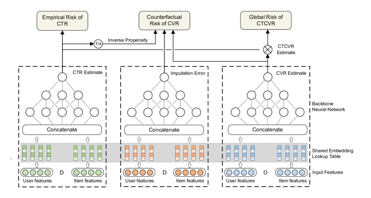
Figure 4: Overview of ESCM², where the ESCM²-IPS consists of the CTR tower and CVR tower; the ESCM²-DR is further augmented by the imputation tower. A common embedding look-up table is shared by all estimators to handle the data sparsity issue.

IV-A2 Doubly Robust Regularizer

Based on (8), the DR regularizer firstly constructs an imputation model $\hat{\delta}_{u,i}$ in (19) to impute the CVR estimation error, and then corrects its imputation with $\hat{e}_{u,i}=\delta_{u,i}-\hat{\delta}_{u,i}$. The imputation is performed in exposure space, whereas the correction is executed in click space where the actual $\delta_{u,i}$ is available. $\hat{e}_{u,i}$ is inversely weighted with the propensity score $q_{u,i}$ to mitigate sample selection bias. In this work, DR regularizer is implemented as

$$\mathcal{R}_{\mathrm{DR}}^{\mathrm{err}}(\phi_{\mathrm{CTR}},\phi_{\mathrm{CVR}},\phi_{\mathrm{IMP}})$$ (23)

$$=\mathbb{E}_{(u,i)\in\mathcal{D}}\left[\hat{\delta}_{u,i}\left(\phi_{\mathrm{IMP}}\right)+\frac{o_{u,i}\hat{e}_{u,i}\left(\phi_{\mathrm{CVR}},\phi_{\mathrm{IMP}}\right)}{q_{u,i}}\right]$$

$$=\frac{1}{|\mathcal{D}|}\sum_{(u,i)\in\mathcal{D}}\hat{\delta}_{u,i}\left(\phi_{\mathrm{IMP}}\right)+\frac{o_{u,i}\hat{e}_{u,i}\left(\phi_{\mathrm{CVR}},\phi_{\mathrm{IMP}}\right)}{\hat{o}_{u,i}\left(\phi_{\mathrm{CTR}}\right)},$$

where $\hat{o}_{u,i}$ in (17) is a surrogate of the propensity score $q_{u,i}$.

Lemma 3.

Let $\mathcal{P}$ be the ideal CVR estimation error in (1), $q_{u,i}$ be the propensity score in (6), $\hat{o}_{u,i}\in\mathbb{R}_{+}$ be the CTR estimate in (17), $\delta_{u,i}$ be the CVR estimation error in (20), $\hat{\delta}_{u,i}$ be the imputation of $\delta_{u,i}$. The bias and variance of $\mathcal{R}_{\mathrm{DR}}^{\mathrm{err}}$ are

$$\operatorname{Bias}\left(\mathcal{R}_{\mathrm{DR}}^{\mathrm{err}}\right) =\frac{1}{|\mathcal{D}|}\left|\sum_{(u,i)\in D}\left(q_{u,i}-\hat{o}_{u,i}\right)\frac{\left(\delta_{u,i}-\hat{\delta}_{u,i}\right)}{\hat{o}_{u,i}}\right|,$$ (24)

$$\mathbb{V}_{O}\left(\mathcal{R}_{\mathrm{DR}}^{\mathrm{err}}\right) =\frac{1}{|\mathcal{D}|^{2}}\sum_{(u,i)\in\mathcal{D}}q_{u,i}\left(1-q_{u,i}\right)\frac{\left(\hat{\delta}_{u,i}-\delta_{u,i}\right)^{2}}{\hat{o}_{u,i}^{2}}.$$

The statistical properties of $\mathcal{R}_{\mathrm{DR}}^{\mathrm{err}}$ are theoretically investigated in Lemma 3, with main observations as follows:

1. Comparing (22) and (24), $\mathcal{R}_{\mathrm{DR}}$ has a lower variance than $\mathcal{R}_{\mathrm{IPS}}$ does given $0<\hat{\delta}_{u,i}<2\delta_{u,i}$.

2. $\mathcal{R}_{\mathrm{DR}}$ is doubly robust since only one of the estimates needs to be accurate to ensure unbiasedness. Specifically, if the propensity estimate is correct, i.e., $\hat{o}_{u,i}=q_{u,i}$, we have $\operatorname{Bias}\left(\mathcal{R}_{\mathrm{DR}}^{\mathrm{err}}\right)=0$ even if the imputation model is wrong. On the flip side, if the imputation model is correct, i.e., $\hat{\delta}_{u,i}=\delta_{u,i}$, we have $\operatorname{Bias}\left(\mathcal{R}_{\mathrm{DR}}^{\mathrm{err}}\right)=0$ even if the propensity estimate is wrong.

The accuracy of $\hat{o}_{u,i}$ can be guaranteed by an arbitrary well-trained CTR estimator; the accuracy of $\hat{\delta}_{u,i}$ can be assured by the auxiliary learning objective as follow:

$$\mathcal{R}_{\mathrm{DR}}^{\mathrm{imp}}(\phi_{\mathrm{CTR}},\phi_{\mathrm{CVR}},\phi_{\mathrm{IMP}})$$ (25)

$$=\mathbb{E}_{(u,i)\in\mathcal{D}}\left[\frac{o_{u,i}\hat{e}^{2}_{u,i}(\phi_{\mathrm{CVR}},\phi_{\mathrm{IMP}})}{\hat{o}_{u,i}\left(\phi_{\mathrm{CTR}}\right)}\right],$$

and the final learning objective of the DR regularizer is

$$\mathcal{R}_{\mathrm{DR}}(\phi_{\mathrm{CTR}},\phi_{\mathrm{CVR}},\phi_{\mathrm{IMP}}) =\mathcal{R}_{\mathrm{DR}}^{\mathrm{err}}(\phi_{\mathrm{CTR}},\phi_{\mathrm{CVR}},\phi_{\mathrm{IMP}})$$ (26)

$$+\mathcal{R}_{\mathrm{DR}}^{\mathrm{imp}}(\phi_{\mathrm{CTR}},\phi_{\mathrm{CVR}},\phi_{\mathrm{IMP}}).$$

IV-B Analytical Properties

This section gives a theoretical demonstration that the suggested counterfactual regularizers effectively handle the IEB and FIP issues. To begin with, Proposition 4 shows that the IPS regularizer in (21) is equivalent to the ideal learning objective in (1), effectively handling the IEB issue.

Proposition 4.

Let $o_{u,i}$ be the click indicator, $\hat{o}_{u,i}$ be the CTR estimate in (17), $q_{u,i}$ be the actual propensity score in (6). Given accurate CTR estimate, i.e., $\hat{o}_{u,i}=q_{u,i}$, $\mathcal{R}_{\mathrm{IPS}}=\mathcal{P}$ holds.

Proof.

$$\mathcal{R}_{\mathrm{IPS}} =\mathbb{E}_{(u,i)\in\mathcal{D}}\left[\frac{o_{u,i}\delta\left(r_{u,i},\hat{r}_{u,i}\right)}{\hat{o}_{u,i}}\right]$$

$$=\frac{|\mathcal{O}|}{|\mathcal{D}|}\mathbb{E}_{(u,i)\in\mathcal{O}}\left[\frac{\delta\left(r_{u,i},\hat{r}_{u,i}\right)}{\hat{o}_{u,i}}\right]$$

$$=\frac{|\mathcal{O}|}{|\mathcal{D}|}\int\frac{\delta\left(r_{u,i},\hat{r}_{u,i}\right)}{\hat{o}_{u,i}}\mathbb{P}(u,i\mid O=1)\,d(u,i)$$

$$=\frac{|\mathcal{O}|}{|\mathcal{D}|}\int\frac{\delta\left(r_{u,i},\hat{r}_{u,i}\right)}{\mathbb{P}(O=1\mid u,i)}\mathbb{P}(u,i\mid O=1)\,d(u,i)$$ (27a)

$$=\int\delta\left(r_{u,i},\hat{r}_{u,i}\right)\mathbb{P}(u,i)\,d(u,i)=\mathcal{P}.$$ (27b)

where (27a) holds because we have $\hat{o}_{u,i}=q_{u,i}$; (27b) is derived by decomposing $\mathbb{P}(u,i\mid O=1)$ with the Bayesian formula. ∎

Notably, Proposition 4 reveals stronger unbiasedness than Proposition 2 through a new proof method. More importantly, it suggests a connection from $\mathcal{R}_{\mathrm{IPS}}$ to the Monte Carlo’s importance sampling [23]. Corollary 5 innovatively and rigorously indicates that $\mathcal{R}_{\mathrm{IPS}}$ is equivalent to importance sampling, which provides solid theoretical supports and inspires substantial theoretical extensions to IPS regularizer [23, 24, 25].

Corollary 5.

$\mathcal{R}_{\mathrm{IPS}}$ is a special practice of importance sampling, which computes the ideal expectation on the exposure space $\mathcal{D}$ with samples in the click space $\mathcal{O}$.

Proof.

Using Bayes’ theorem, (27a) could be reformulated as

$$\int\delta\left(r_{u,i},\hat{r}_{u,i}\right)\frac{\mathbb{P}(u,i)}{\mathbb{P}(u,i\mid O=1)}\mathbb{P}(u,i\mid O=1)\,d(u,i),$$ (28)

which is a importance sampling to estimate the expectation of $\delta(r_{u,i},\hat{r}_{u,i})$ in $\mathbb{P}(u,i)$, based on the samples from $\mathbb{P}(u,i\mid O=1)$. The importance weight is $\mathbb{P}(u,i)/\mathbb{P}(u,i\mid O=1)$. ∎

Second, $\mathcal{R}_{\mathrm{IPS}}$ handles the FIP issue with ESMM. This claim is supported by Proposition 6: it encourages to estimate CVR as $\mathbb{P}\left(r_{u,i}=1\mid do\left(o_{u,i}=1\right)\right)$ in (15), which models the dependency from click to conversion explicitly, thus mitigating the FIP issue with ESMM.

Proposition 6.

Let $\mathbb{P}\left(r_{u,i}=1\mid do\left(o_{u,i}=1\right)\right)$ be the counterfactual conversion rate assuming the user clicked the item, $\hat{r}^{\mathrm{IPS}}_{u,i}$ be the CVR estimate with $\mathcal{R}_{\mathrm{IPS}}$ in (21). For all exposed user-item intersections, (21) encourages:

$$\hat{r}_{u,i}^{\mathrm{IPS}}\rightarrow\mathbb{P}\left(r_{u,i}=1\mid do\left(o_{u,i}=1\right)\right).$$ (29)

Proof.

We start by dividing the user-item intersections in the exposure space into $K$ clusters $\{L_{k}\}_{k=1}^{\mathrm{K}}$. Since the characteristics of user-item intersections in each cluster $L_{k}$ are similar, it is reasonable to assume that conditional exchangeability [22] holds in each cluster. Formally, within the cluster $L_{k}$, the empirical distribution of clicks is independent of the distributions of counterfactual CVR estimation errors:

$$\{\delta^{(1)}_{k},\delta^{(0)}_{k}\}\upmodels O_{k},$$ (30)

where $\delta^{(1)}_{k}$ is the distribution of counterfactual CVR errors in $L_{k}$ assuming all users clicked the items, i.e., $o_{u,i}=1$ holds for all $(u,i)\in L_{k}$, $\delta^{(0)}_{k}$ is that given all users unclicked the items, i.e., $o_{u,i}=0$ holds for all $(u,i)\in L_{k}$.

Then, based on the law of iterated expectations we have

$$\mathcal{R}_{\mathrm{IPS}}=\mathbb{E}_{(u,i)\in\mathcal{D}}\left[\frac{o_{u,i}\delta_{u,i}}{\hat{o}_{u,i}}\right]=\mathbb{E}_{k}\left\{\mathbb{E}_{(u,i)\in L_{k}}\left[\frac{o_{u,i}}{\hat{o}_{u,i}}\delta_{u,i}\right]\right\},$$ (31)

and within the cluster $L_{k}$ we have:

$$\mathbb{E}_{(u,i)\in L_{k}}\left[\frac{o_{u,i}}{\hat{o}_{u,i}}\delta_{u,i}\right] =\mathbb{E}_{(u,i)\in L_{k}}\left[\frac{o_{u,i}}{\hat{o}_{u,i}}\delta_{u,i}^{(1)}\right]$$ (32a)

$$=\mathbb{E}_{(u,i)\in L_{k}}\left[\frac{o_{u,i}}{\hat{o}_{u,i}}\right]\mathbb{E}_{(u,i)\in L_{k}}\left[\delta_{u,i}^{(1)}\right]$$ (32b)

$$=\mathbb{E}_{(u,i)\in L_{k}}\left[\delta_{u,i}^{(1)}\right]\triangleq\Delta_{k},$$ (32c)

where (32a) and (32b) holds as we have (30); $\Delta_{k}$ is the expectation of $\delta_{k}^{(1)}$. According to (32c) and (31) we have

$$\mathcal{R}_{\mathrm{IPS}}=\mathbb{E}_{k}\left[\Delta_{k}\right].$$ (33)

Therefore, minimizing $\mathcal{R}_{\mathrm{IPS}}$ is equivalent to minimizing $\Delta_{k}$ in clusters $k=1,2,...,K$; and minimizing $\Delta_{k}$ encourages the convergence of the CVR estimate $\hat{r}_{u,i}^{\mathrm{IPS}}$ to the actual CVR assuming click takes place for all user-item intersections in the $k$-th cluster. The proof is completed. ∎

Finally, the proposed doubly robust regularizer $\mathcal{R}_{\mathrm{DR}}$ also mitigates the IEB and FIP issues, because these theoretical results also apply to it. The formal justification is provided in Proposition 7-8.

IV-C Architecture and learning objective

The general architecture of ESCM² in Fig. 4 exploits the sequential user behavior track, i.e., exposure$\rightarrow$click$\rightarrow$ conversion with a multitask learning framework. The learned representations are shared among tasks through a common look-up embedding table which effectively alleviates the data sparsity issue [4, 15, 16]. We utilize a CTR tower to estimate $\hat{o}_{u,i}$ in (17), a CVR tower to estimate $\hat{r}_{u,i}$ in (18), and an imputation tower to impute $\hat{\delta}_{u,i}$ in (19).

The learning objective of ESCM² includes three terms

$$\mathcal{L}_{\mathrm{ESCM^{2}}}:=\mathcal{L}_{\mathrm{CTR}}+\lambda_{\mathrm{c}}\mathcal{L}_{\mathrm{CVR}}+\lambda_{\mathrm{g}}\mathcal{L}_{\mathrm{CTCVR}},$$ (34)

where $\mathcal{L}_{\mathrm{CTR}}$ is the empirical risk of CTR estimation, $\mathcal{L}_{\mathrm{CTCVR}}$ is the global risk of CTCVR estimation; $\mathcal{L}_{\mathrm{CVR}}$ is the counterfactual risk of CVR estimation; $\lambda_{\mathrm{c}}$ and $\lambda_{\mathrm{g}}$ are weighting factors. Specifically, the empirical CTR risk $\mathcal{L}_{\mathrm{CTR}}$ is computed in the exposure space $\mathcal{D}$ as

$$\mathcal{L}_{\mathrm{CTR}}(\phi_{\mathrm{CTR}})=\mathbb{E}_{(u,i)\in\mathcal{D}}\left[\delta\left(o_{u,i},\hat{o}_{u,i}\left(x_{u,i};\phi_{\mathrm{CTR}}\right)\right)\right],$$ (35)

where $\delta$ is implemented with binary cross-entropy in this study. The global CTCVR risk $\mathcal{L}_{\mathrm{CTCVR}}$ is computed as

$$\mathcal{L}_{\mathrm{CTCVR}}(\phi_{\mathrm{CTR}},\phi_{\mathrm{CVR}})$$ (36)

$$=\mathbb{E}_{(u,i)\in\mathcal{D}}\left[\delta\left(o_{u,i}r_{u,i},\hat{o}_{u,i}\left(x_{u,i};\phi_{\mathrm{CTR}}\right)\hat{r}_{u,i}\left(x_{u,i};\phi_{\mathrm{CVR}}\right)\right)\right].$$

Finally, based on the specific formulations of $\mathcal{L}_{\mathrm{CVR}}$, two implementations of ESCM² are devised:

• ESCM²-IPS, which employs a CTR tower in (17) and a CVR tower in (18) to calculate $\mathcal{L}_{\mathrm{CVR}}$ with $\mathcal{R}_{\mathrm{IPS}}$ in (21).

• ESCM²-DR, which employs an extra imputation tower in (19), and calculates $\mathcal{L}_{\mathrm{CVR}}$ with $\mathcal{R}_{\mathrm{DR}}$ in (26).

V Experiments

In this section, extensive experiments are conducted to investigate the research questions as follows:
RQ1: How does ESCM² perform compared to the prevalent CVR and CTCVR estimators in offline and online scenarios?
RQ2: Does ESMM suffer from the inartistic estimation bias on CVR estimation? Does ESCM² effectively reduce the bias?
RQ3: Does ESMM inject false independence prior in CTCVR estimation? Does ESCM² mitigate this problem?
RQ4: How to tune the weights of learning objectives? Is the performance of ESCM² sensitive to it?

V-A Setup

V-A1 Benchmarks

• Industrial benchmark is constructed with our industrial recommendation logs in 90 days, divided for training, validation and test in a chronological order. Negative samples are downsampled in the training phase to maintain an approximate exposure:click:conversion ratio of 100:10:1.

• Public benchmark is set to Ali-CCP dataset for reproducibility consideration. Only single-valued categorical fields are employed following prevalent settings [26], and 10% of the training set are saved for validation. Details of both benchmarks are summarized in Table I.

TABLE I: Benchmark description.

Name	# Train	# Valid	# Test	# User	# Click	# Conversion
Industrial	61.58M	0.39M	24.28M	37.73M	3.73M	0.32M
Ali-CCP	33.12M	3.67M	37.64M	0.25M	1.42M	7.92K

V-A2 Baselines

Since recommender’s performance can be largely enhanced through Multi-Task Learning (MTL) [14, 16], single-task CVR estimation approaches [12, 18] are excluded from our baselines for fairness consideration. We start with two prevalent methods which co-train CTR and CVR estimators and share the embeddings between them:

• Naïve [27] optimizes the CTR estimator with (35), and the CVR estimator with the biased approach in (3).

• MTL-IMP [4] is the same as the Naïve approach, except that the unclicked samples are added as negative samples to train the CVR estimator.

• ESMM⁴ [4] avoids the direct training of CVR estimator and thus circumventing the sample selection bias.

Both methods above induce sample selection bias, which leads to sub-optimal performance of CVR and CTCVR estimation [4]. As a result, it is essential to expand our scope of baselines to debiased methods as follows:

• MTL-EIB [19] imputes the CVR estimation error for all samples and corrects its imputation with clicked samples to get theoretically unbiased CVR estimation.

• MTL-IPS [14] integrates the IPS approach [12] in a multitask learning framework, which is a theoretically unbiased CVR estimator.

• MTL-DR⁵ [14] incorporates the DR approach [18] in a multitask learning framework, which is a theoretically unbiased and robust CVR estimator.

V-A3 Training Protocol

For all methods in comparison, the multi-gate mixture of expert model [27] is employed as backbone to implement (17)-(19). The learning rate and weight decay are set to 1e^-4 and 1e^-3, respectively; with other optimizer settings consistent with Adam optimizer [28] to make the results comparable. The weighting factors $\lambda_{\mathrm{g}}$ and $\lambda_{\mathrm{c}}$ are set to 1 and 0.1, respectively, based on the parameter study in Section V-F. The embeddings of size 5 are shared across tasks to handle the data sparsity issue. The performance is checked every 1 thousand iterations over the validation dataset, and the best model is evaluated on the test dataset.

V-A4 Evaluation Protocol

We mainly use the area under roc (AUC) metric to compare the ranking performance of models. Nevertheless, it only reveals the ranking performance that is averaged at all thresholds. To better understand the performance of each model, we also report the model performance for the best threshold on the receiver operating characteristic curve and the recall and F1 scores for the best threshold on the precision-recall curve, respectively.

TABLE II: Offline comparison of CVR estimation performance (mean±std).

Benchmark	Industrial Benchmark					Ali-CCP Benchmark
Model	Recall	F1	KS	AUC		Recall	F1	KS	AUC
Naïve	0.5789±0.0071	0.3344±0.0052	0.3872±0.0043	0.7515±0.0164		0.2854±0.0050	0.0991±0.0053	0.1123±0.0056	0.5987±0.0139
ESMM	0.5742±0.0055	0.6330±0.0074	0.3856±0.0051	0.7547±0.0183		0.2968±0.0036	0.1157±0.0084	0.1267±0.0043	0.6071±0.0133
MTL-EIB	0.5121±0.0072	0.5808±0.0048	0.3371±0.0051	0.7272±0.0140		0.2372±0.0043	0.0825±0.0051	0.0717±0.0057	0.5603±0.0135
MTL-IMP	0.5841±0.0092	0.1272±0.0040	0.3974±0.0047	0.7563±0.0114		0.2962±0.0056	0.1135±0.0055	0.1163±0.0043	0.6114±0.0137
MTL-IPS	0.5651±0.0068	0.6810±0.0042	0.3960±0.0048	0.7586±0.0112		0.2975±0.0070	0.0941±0.2163	0.1177±0.0063	0.6091±0.0123
MTL-DR	0.5137±0.0081	0.6804±0.0042	0.4016±0.0046	0.7579±0.0135		0.2953±0.0178	0.1159±0.0084	0.1255±0.0141	0.6065±0.0172
ESCM2-IPS	0.5932±0.0094	0.7161±0.0089∗	0.4144±0.0051∗	0.7730±0.0150		0.3061±0.0059	0.1180±0.0047	0.1312±0.0060	0.6163±0.0151
ESCM2-DR	0.5986±0.0068∗	0.6884±0.0052	0.4119±0.0050	0.7679±0.0113		0.3095±0.0054∗	0.1315±0.0053∗	0.1393±0.0042∗	0.6142±0.0133

• 1. The underline marks the best performance for each metric across all baseline models.

• 2. “*” marks the metrics of significant improvement in ESCM² relative to the best baselines, with p-value $<$ 0.01 in the paired samples t-test.

TABLE III: Offline comparison of CTCVR estimation performance (mean±std).

Benchmark	Industrial Benchmark					Ali-CCP Benchmark
Model	Recall	F1	KS	AUC		Recall	F1	KS	AUC
Naïve	0.6602	1.0048	0.4631	0.7954		0.2921	0.0978	0.1192	0.6003
ESMM	0.6819	1.1062	0.4827	0.8153		0.3027	0.1139	0.1292	0.6081
MTL-EIB	0.5975	0.8458	0.4220	0.7912		0.2542	0.0959	0.0697	0.5699
MTL-IMP	0.5880	1.3393	0.4126	0.7752		0.2973	0.1110	0.1264	0.6087
MTL-IPS	0.6716	1.0653	0.4840	0.8044		0.2911	0.1044	0.1302	0.6138
MTL-DR	0.6684	1.1707	0.4844	0.8106		0.2980	0.1096	0.1360	0.6130
ESCM2-IPS	0.6804	1.1753	0.4991	0.8198		0.3184∗	0.1207∗	0.1436	0.6189
ESCM2-DR	0.7013∗	1.2842	0.5134∗	0.8265		0.3117	0.1180	0.1494	0.6245

• 1. The underline marks the best performance across all baselines.

• 2. “*” marks the metrics of significant improvement in ESCM² relative to the best baselines, with p-value $<$ 0.01 in the paired samples t-test.

V-B Performance Comparison

The performance of ESCM² on CVR and CTCVR estimation is compared with its competitors on both offline benchmarks. The CVR estimation performance is detailed in Table II, with mean and standard deviation reported over 10 random seeds. Notable findings are summarized as follows:

• The biased approaches show competitive performance on both benchmarks. In particular, the AUCs of ESMM and Naïve estimator reach 0.754 and 0.751, respectively, on the industrial benchmark.

• Most of the unbiased baselines outperform the biased methods on both benchmarks. In particular, MTL-IPS reaches the highest AUC and F1 scores of all baselines on the industrial benchmark, enhancing the AUC and KS scores of ESMM by 0.39% and 1.04%, respectively. These results reveal the prospect of incorporating an unbiased estimator to ESMM for better ranking performance.

• The developed ESCM² significantly enhances the performance based on the best baselines. This improvement is credited to the mitigation of the IEB and FIP issues, and the effectiveness of the entire-space modelling paradigm.

On top of CVR, a more prevalent ranking metric is CTCVR in industry, which accounts for both clicks and conversions. As a result of mitigating the IEB and FIP defects, we anticipate the improvement of CTCVR estimation and thus that of business metrics and real-world benefits. The CTCVR estimation performance is reported in Table III, and notable observations are summarized as follows⁶:

• ESMM exhibits competitive CTCVR estimation performance across all baseline methods. It achieves the advanced recall and F1 scores on the AliCCP benchmark, as well as the top recall and AUC scores on the industrial benchmark. This advance could be attributed to the explicit inclusion of training CTCVR estimator in ESMM’s learning objective. Due to the excellence in CTCVR estimation, it has been extensively employed in numerous business scenarios.

• ESCM² outperforms rivals on the CTCVR estimation task, albeit less significantly than on the CVR estimation task. In particular, ESCM²-IPS reaches the top recall and F1 scores on AliCCP, and ESCM²-DR gets the highest KS and AUC on the industrial benchmark. The superiority of ESCM² could be attributed to the incorporation of training CTCVR estimators in its learning objective (36), as well as elimination of IEB and PIP issues through regularizers (21) and (23).

V-C Online A/B Test

TABLE IV: Overview of Online A/B comparison in 3 scenarios

Scenario	# UV	# PV	# Order	# Premium	CVR	CTCVR
1	2.2M	3.1M	+2.84%	+10.85%	+5.64%	+3.92%
2	3.4M	4.9M	+4.26%	+3.88%	+0.43%	+1.75%
3	125K	136K	+40.55%	+12.69%	-	-

TABLE V: Comprehensive Online A/B results in Scenario 1

Metrics	Day 1	Day 2	Day 3	Day 4	Day 5	Day 6
# Order	-9.76%	-1.85%	-1.43%	+9.07%	+0.73%	+6.26%
# Premium	+64.53%	+37.47%	+22.09%	-12.49%	+4.26%	+11.10%
UV-CVR	+7.25%	-1.66%	+9.39%	+8.58%	+2.51%	+8.62%
UV-CTCVR	+0.20%	-3.50%	+2.50%	+9.48%	+2.75%	+6.64%

To further demonstrate the advantage of ESCM² over ESMM, online experiments are conducted on the real-world recommendation systems in Alipay. We first implement ESMM and ESCM² using our C$++$ based machine learning engine and open data processing service. The IPS regularizer (21), with better training efficiency and a smaller scale of parameters, is selected to implement ESCM² for online serving. Then, unique visitors (UV) are randomly assigned into two buckets, each of which is served by either ESMM or ESCM². Finally, we compare the model performance using our A/B experiment board, where the considered metrics mainly include UV-CVR, UV-CTCVR, order quantity (# Order) and actual premium (# Premium). We conduct the online comparison within 3 large-scale scenarios. Table IV gives an overview of experiment results, with detailed analysis as follows:

• The first scenario is the insurance recommendation from Alipay. This experiment lasts six days and encompasses about 3.1 million page views (PVs) and 2.2 million UVs. ESCM² increases actual premium by 10.85% and order quantity by 2.84%. Another noteworthy point is that UV-CVR and UV-CTCVR increased significantly by 5.64% and 3.92%, respectively. An additional daily comparison is performed in Table V, where ESCM² is always superior to ESMM in most metrics.

• The second scenario is the same but newly renovated insurance recommendation from Alipay, lasting six days, encompassing about 4.9 million PVs and 3.4 million UVs. Overall, ESCM² enhances the the premium by 3.88% and order quantity by 4.26%. A substantial rise of 0.43% for UV-CVR and 1.75% for UV-CTCVR is also observed.

• The third scenario is our Wufu campaign, which contains around 136 thousand PVs and 125 thousand UVs over the period of four days. A huge improvement of 40.55% for order quantity and 12.69% for premium is witnessed.

V-D Additional Study on Intrinsic Estimation Bias

In this section, we investigate the IEB issue with ESMM and the superiority of ESCM² to handle this issue. The field ”Label” in Table VI displays the average of the actual CVR in the click space, which upper bounds the average actual CVR in the exposure space that we care for. Comparing it with the average CVR estimates over the exposure space reveals the lower-bound of CVR estimation bias. Several meaningful observations are noted.

First, the CVR estimates provided by ESMM are consistently higher than the actual values. On the industrial trainset, for instance, the actual CVR average does not surpass 0.095, whereas the ESMM reaches 0.158. For the test set, an overestimation of 0.124 is also observed. These observations back up the existence of IEB that we detail in Proposition 1.

Second, ESCM² alleviates the IEB issue, which verifies our claims in Proposition 4. On the industrial benchmark, for instance, ESCM²-IPS decreases the average estimation error by around 0.031 (0.035) on the training (test) set; ESCM²-DR reduces the error by 0.037 (0.045) on the training (test) set.

TABLE VI: Average of the actual and estimated CVR values.

Benchmark	Subset	Label	ESMM	ESCM2-IPS	ESCM2-DR
Ali-CCP	Train	0.0055	0.0101±0.0011	0.0059±0.0005	0.0076±0.0018
Ali-CCP	Test	0.0056	0.0113±0.0008	0.0060±0.0009	0.0059±0.0009
Industry	Train	0.0953	0.1588±0.0107	0.1277±0.0053	0.1216±0.0093
Industry	Test	0.0407	0.1643±0.0095	0.1290±0.0092	0.1188±0.0022

V-E Additional Study on False Independence Prior

The FIP issue is that the model fails to portray the intrinsic causation between clicks and conversions, as represented by the missing edge O$\rightarrow$R in Fig. 3 (a). In this section, the existence of FIP issue is illustrated by calculating the strength of causation from click to conversion. Noting that the causation cannot be measured directly with statistical methods (e.g., Pearson coefficient) due to the inclusion of confounders in Fig. 3. The data is thus pre-processed with the propensity score matching technique, following the implementation details in reference [29] to handle the confounding effects. Then, it is feasible to estimate the causation strength from data with causal risk ration (CRR) [30]. Briefly, causation gets significant as CRR approaches 1, and vice versa. As a result, the causation strength is represented as the absolute deviation between 1 and CRR.

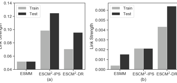
Figure 5: The strength of causal link O $\rightarrow$ R, which is measured by the absolute deviation between 1 and CRR on (a) industrial benchmark and (b) Ali-CCP.

The causation strengths between the CTR estimates and the CVR estimates from different models are compared in Fig. 5. The trivial causation strength of ESMM, such as around 0.05 (resp. 0.001) on the industrial (resp. Ali-CCP) benchmark, supports the existence of the FIP issue in Section III-B. In contrast, ESCM² augments the causation strength significantly and hence handle the FIB issue effectively, which confirms Proposition 6. The ESCM²-IPS, for instance, exceeds 0.12 (resp. 0.002) on the industrial (resp. Ali-CCP) benchmark.

V-F Hyper-parameter Tuning and Ablation Study

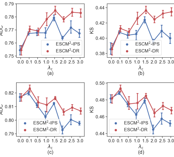
Figure 6: Performance of CVR (a-b) and CTCVR estimation (c-d) with different settings of counterfactual risk weight $\lambda_{\mathrm{c}}$.

Two crucial hyperparameters of ESCM² are the weighting factors (i.e., $\lambda_{\mathrm{c}}$ and $\lambda_{\mathrm{g}}$) in the learning objective (34). In this section, they are tuned within the range [0, 3] to investigate the impact of causal regularization and global risk minimization on the performance of CVR and CTCVR estimation.

The weighting factor $\lambda_{\mathrm{c}}$ of causal regularization is investigated in Fig. 6. Evidently, enlarging $\lambda_{\mathrm{c}}$ consistently benefits CVR estimation, which showcases the effectiveness of causal regularization. The AUC of ESCM²-DR, for instance, grows from 0.755 at $\lambda_{\mathrm{c}}=0$ where the causal regularization is invalid, to around 0.785 at $\lambda_{\mathrm{c}}=1.5$. Additionally, causal regularization also benefits CTCVR estimates. For example, the AUC of ESCM²-IPS boosts from 0.817 at $\lambda_{\mathrm{c}}=0$ to 0.821 at $\lambda_{\mathrm{c}}=0.1$. Nevertheless, the overemphasis on CVR risk has a negative impact on CTCVR estimation. For example, a drop in AUC by 0.012 is observed for ESCM²-IPS from $\lambda_{\mathrm{c}}=0.1$ to $\lambda_{\mathrm{c}}=3.0$. It is speculated to the seesaw effect in multitask learning [31], i.e., overemphasis on the CVR risk misleads the optimizer to ignore the CTR risk, thus leads to suboptimal CTR and CTCVR estimation performance. Therefore, we suggest tuning $\lambda_{\mathrm{c}}$ within the range [0, 0.1].

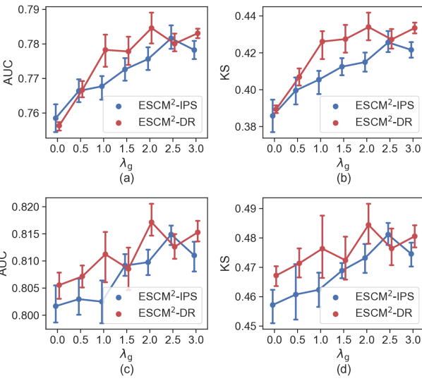
Figure 7: Performance of CVR (a-b) and CTCVR estimation (c-d) with different settings of global risk weight $\lambda_{\mathrm{g}}$.

The weighting factor $\lambda_{\mathrm{g}}$ of global risk is studied in Fig. 7. In short, increasing $\lambda_{\mathrm{g}}$ within the range [0, 3] is beneficial for both CTR and CTCVR estimation. In the CVR estimation task, for instance, increasing $\lambda_{\mathrm{g}}$ from 0 to 2.5, the KS of ESCM²-DR climbs from 0.385 to about 0.434; the AUC of ESCM²-IPS grows by 0.023, significantly. These observations verify the effectiveness of entire space multitask modelling paradigm, exploiting the sequential user behavior track as per Fig. 2.

VI Related work

Modelling the user behaviors with inter-dependency is a tough research problem in recommendation system since the dependencies inevitably lead to MNAR feedback labels [12, 32]. In terms of the methods utilized to handle the MNAR problem in CVR estimation task, current efforts in this domain can be broadly classified into two groups.

VI-A Decomposition Approach

One line of the works is performing behavior decomposition over exposure space. Initially, ESMM [4] breaks CTCVR down into CTR and CVR, and optimizes CVR estimator implicitly by optimizing the CTR and CTCVR estimators over exposure space. On the basis, ESM² [15] enhances the probability decomposition by incorporating extra post-click purchase-related actions. HEROES [33] further proposes to automatically discover the multi-scale patterns of user behaviors. As the number of user actions under consideration rises, their interactions become more complicated and cannot be depicted by Markov chain. GMCM [34] encodes user micro behaviors as graphs and establishes a graph convolution network to model their interactions. HM³ [35] considers more user behaviors and introduces a sequential behavior graph to capture the interdependence among them. Noting that these methods are model-agnostic, emerging model architectures [31, 36, 37] for effectively sharing representations among tasks. Despite their evolutionary performance in industrial user behavior modelling, these approaches circumvent the MNAR problem and thus suffers from the funneling effect and estimation bias.

VI-B Causal Recommendation Approach

Another line of the works seeks to handle the MNAR issue directly with causal inference techniques, which has attracted a great deal of interest [38]. We concentrate on methods based on propensity scores since they are prevalent in the context of CVR estimation. Initially, Schnabel et al. [12] developed an IPS-based unbiased training and evaluation method that constructs unbiased estimators with biased recommendation data, handling the MNAR problem directly. Wang et al. [18] investigates the application of doubly robust methods in recommendation and presents a thorough theoretical explanation that motivates a multitude of robust extensions [39, 40, 41, 42]. Zhang et al. [14] develops a multitask learning framework to estimate CTR and unbiased CVR simultaneously. More recently, Le et al. [43] further considers the MNAR effect of unclicked events, and constructs a dual learning architecture that re-weights both the clicked and unclicked events to handle this issue.

VII Conclusion

The entire space multitask learning paradigm is prevalent in many real-world industrial practices due to its efficacy of modeling user behavior dependency. Nevertheless, two defects, namely intrinsic estimation bias and false independence prior, have long been neglected. This study begins with demonstrating the existence of the two issues explicitly. Then, a principled approach named ESCM² is developed, which handles both problems through an additional counterfactual regularizer. Finally, real-world experiments demonstrate that ESCM² alleviates both issues to a significant degree and achieves superior performance against baseline methods.

There are two open questions that we leave for future research. First, only the sequential track of user behaviors in Fig. 2 is considered in this study; however, in many industrial scenarios, the dependency among user behaviors are more complex than Markov chains. Although some studies [15, 34] extend ESMM to describe such complex dependency, they also inevitably suffers from both IEB and FIP defects. Leveraging the counterfactual regularization techniques in ESCM², these methods coud be further enhanced by handling both defects.

Another open question is to avoid the fragility of propensity score. The unbiasedness of re-weighting methods (i.e., IPS and DR) is highly dependent on the accuracy of propensity score (i.e., CTR) model. Nonetheless, CTR estimation remains a challenging topic in recommendation system. As a result, it is tempting to replace the re-weighting paradigm in this study with adversarial training [44] and representation learning [45] to balance the exposure space and click space directly.

Acknowledgement. The Zhejiang University Team is supported by National Natural Science Foundation of China (62073288, 12075212, 12105246). We are also pleased to thank the Ant Group for providing their expertise in the data preparation, offline evaluation and online A/B test phases.

Lemma 2.

Let $\mathcal{P}$ be the ideal CVR estimation error in (1), $q_{u,i}$ be the propensity score in (6), $\hat{o}_{u,i}$ be the CTR estimate in (17), $\delta_{u,i}$ be the CVR estimation error in (20). The bias and variance of $\mathcal{R}_{\mathrm{IPS}}$ are

$$\operatorname{Bias}\left(\mathcal{R}_{\mathrm{IPS}}\right) =\frac{1}{|\mathcal{D}|}\left|\sum_{(u,i)\in D}\delta_{u,i}\left(\frac{q_{u,i}}{\hat{o}_{u,i}}\right)\right|,$$ (37)

$$\mathbb{V}_{O}\left(\mathcal{R}_{\mathrm{IPS}}\right) =\frac{1}{|\mathcal{D}|^{2}}\sum_{(u,i)\in\mathcal{D}}\frac{q_{u,i}\left(1-q_{u,i}\right)}{\hat{o}_{u,i}^{2}}\left(\delta_{u,i}\right)^{2}.$$

Proof.

$$\operatorname{Bias}\left[\mathcal{R}_{\mathrm{IPS}}\right] =\left|\mathbb{E}_{O}\left[\mathcal{R}_{\mathrm{IPS}}\right]-\mathcal{P}\right|$$ (38)

$$=\left|\frac{1}{|\mathcal{D}|}\sum_{(u,i)\in\mathcal{D}}\mathbb{E}_{O}\left[\frac{o_{u,i}\delta_{u,i}}{\hat{o}_{u,i}}\right]-\delta_{u,i}\right|$$

$$=\left|\frac{1}{|\mathcal{D}|}\sum_{(u,i)\in\mathcal{D}}\left[\frac{q_{u,i}\delta_{u,i}}{\hat{o}_{u,i}}-\delta_{u,i}\right]\right|$$

$$=\frac{1}{|\mathcal{D}|}\left|\sum_{(u,i)\in D}\delta_{u,i}\left(\frac{q_{u,i}}{\hat{o}_{u,i}}\right)\right|$$

$$\mathbb{V}_{O}\left[\mathcal{R}_{\mathrm{IPS}}\right] =\frac{1}{|\mathcal{D}|^{2}}\sum_{(u,i)\in\mathcal{D}}\mathbb{V}_{O}\left[\frac{o_{u,i}\delta_{u,i}}{\hat{o}_{u,i}}\right]$$ (39)

$$=\frac{1}{|\mathcal{D}|^{2}}\sum_{(u,i)\in\mathcal{D}}\mathbb{V}_{O}\left[o_{u,i}\right]\cdot\left(\frac{\delta_{u,i}}{\hat{o}_{u,i}}\right)^{2}$$

$$=\frac{1}{|\mathcal{D}|^{2}}\sum_{(u,i)\in\mathcal{D}}\frac{q_{u,i}\left(1-q_{u,i}\right)}{\hat{o}_{u,i}^{2}}\left(\delta_{u,i}\right)^{2}.$$

∎

Lemma 3.

Let $\mathcal{P}$ be the ideal CVR estimation error in (1), $q_{u,i}$ be the propensity score in (6), $\hat{o}_{u,i}$ be the CTR estimate in (17), $\delta_{u,i}$ be the CVR estimation error in (20), $\hat{\delta}_{u,i}$ be the imputation of $\delta_{u,i}$. The bias and variance of $\mathcal{R}_{\mathrm{DR}}^{\mathrm{err}}$ are

$$\operatorname{Bias}\left(\mathcal{R}_{\mathrm{DR}}^{\mathrm{err}}\right) =\frac{1}{|\mathcal{D}|}\left|\sum_{(u,i)\in D}\left(q_{u,i}-\hat{o}_{u,i}\right)\frac{\left(\delta_{u,i}-\hat{\delta}_{u,i}\right)}{\hat{o}_{u,i}}\right|,$$ (40)

$$\mathbb{V}_{O}\left(\mathcal{R}_{\mathrm{DR}}^{\mathrm{err}}\right) =\frac{1}{|\mathcal{D}|^{2}}\sum_{(u,i)\in\mathcal{D}}q_{u,i}\left(1-q_{u,i}\right)\frac{\left(\hat{\delta}_{u,i}-\delta_{u,i}\right)^{2}}{\hat{o}_{u,i}^{2}}.$$

Proof.

$$\begin{aligned} \operatorname{Bias}\left[\mathcal{R}_{\mathrm{DR}}^{\mathrm{err}}\right]&=\left|\mathbb{E}_{O}\left[\mathcal{R}_{\mathrm{DR}}^{\mathrm{err}}\right]-\mathcal{P}\right|\\ &=\left|\frac{1}{|\mathcal{D}|}\sum_{(u,i)\in\mathcal{D}}\mathbb{E}_{O}\left[\hat{\delta}_{u,i}+\frac{o_{u,i}\left(\delta_{u,i}-\hat{\delta}_{u,i}\right)}{\hat{o}_{u,i}}\right]-\delta_{u,i}\right|\\ &=\left|\frac{1}{|\mathcal{D}|}\sum_{(u,i)\in\mathcal{D}}\left[\hat{\delta}_{u,i}+\frac{q_{u,i}\left(\delta_{u,i}-\hat{\delta}_{u,i}\right)}{\hat{o}_{u,i}}-\delta_{u,i}\right]\right|\\ &=\frac{1}{|\mathcal{D}|}\left|\sum_{(u,i)\in D}\frac{q_{u,i}-\hat{o}_{u,i}}{\hat{o}_{u,i}}\left(\delta_{u,i}-\hat{\delta}_{u,i}\right)\right|\end{aligned}$$ (41)

$$\mathbb{V}_{O}\left[\mathcal{R}_{\mathrm{DR}}^{\mathrm{err}}\right] =\frac{1}{|\mathcal{D}|^{2}}\sum_{(u,i)\in\mathcal{D}}\mathbb{V}_{O}\left[\hat{\delta}_{u,i}+\frac{o_{u,i}\left(\delta_{u,i}-\hat{\delta}_{u,i}\right)}{\hat{o}_{u,i}}\right]$$ (42)

$$=\frac{1}{|\mathcal{D}|^{2}}\sum_{(u,i)\in\mathcal{D}}\mathbb{V}_{O}\left[o_{u,i}\right]\cdot\left(\frac{\delta_{u,i}-\hat{\delta}_{u,i}}{\hat{o}_{u,i}}\right)^{2}$$

$$=\frac{1}{|\mathcal{D}|^{2}}\sum_{(u,i)\in\mathcal{D}}\frac{q_{u,i}\left(1-q_{u,i}\right)}{\hat{o}_{u,i}^{2}}\left(\hat{\delta}_{u,i}-\delta_{u,i}\right)^{2}.$$

∎

Proposition 7.

Let $o_{u,i}$ be the click indicator, $\hat{o}_{u,i}$ be the CTR estimate in (17), $q_{u,i}$ be the actual propensity score in (6), $\hat{\delta}_{u,i}$ be the imputed CVR error in (19). Given accurate CTR estimate, i.e., $\hat{o}_{u,i}=q_{u,i}$ or imputation model, i.e., $\hat{\delta}_{u,i}=\delta_{u,i}$, we have $\mathcal{R}_{\mathrm{DR}}^{\mathrm{err}}=\mathcal{P}$.

Proof.

First, given accurate imputation model, i.e., $\hat{\delta}_{u,i}=\delta_{u,i}$ and $\hat{e}_{u,i}=0$, (23) degrades to

$$\mathcal{R}_{\mathrm{DR}}^{\mathrm{err}}=\int\delta\left(r_{u,i},\hat{r}_{u,i}\right)\mathbb{P}(u,i)\,d(u,i)=\mathcal{P}.$$ (43)

Second, given accurate propensity model, i.e., $\hat{o}_{u,i}=q_{u,i}$, following (27) we have

$$\ \ \ \mathbb{E}_{(u,i)\in\mathcal{D}}\left[\frac{o_{u,i}\hat{e}_{u,i}\left(\phi_{\mathrm{CVR}},\phi_{\mathrm{IMP}}\right)}{\hat{o}_{u,i}}\right]$$ (44)

$$=\mathbb{E}_{(u,i)\in\mathcal{D}}\left[\frac{o_{u,i}\hat{e}_{u,i}\left(\phi_{\mathrm{CVR}},\phi_{\mathrm{IMP}}\right)}{q_{u,i}}\right]$$

$$=\int\hat{e}_{u,i}\mathbb{P}(u,i)d(u,i),$$

, and (23) can be simplified as

$$\mathcal{R}_{\mathrm{DR}}^{\mathrm{err}} =\int\left(\hat{\delta}_{u,i}+\hat{e}_{u,i}\right)\mathbb{P}(u,i)d(u,i)$$ (45)

$$\mathcal{R}_{\mathrm{DR}}^{\mathrm{err}} =\int\left(\delta_{u,i}\right)\mathbb{P}(u,i)d(u,i)=\mathcal{P}.$$

As such, either $\hat{o}_{u,i}=q_{u,i}$ or $\hat{\delta}_{u,i}=\delta_{u,i}$ makes $\mathcal{R}_{\mathrm{DR}}^{\mathrm{err}}=\mathcal{P}$, the proof is completed. ∎

Proposition 8.

Let $\mathbb{P}\left(r_{u,i}=1\mid do\left(o_{u,i}=1\right)\right)$ be the counterfactual conversion rate ”assuming” the user clicked the item, $\hat{r}^{\mathrm{DR}}_{u,i}$ be the CVR estimate with DR regularizer (23). For all exposed user-item intersections, (23) encourages:

$$\hat{r}_{u,i}^{\mathrm{DR}}\rightarrow\mathbb{P}\left(r_{u,i}=1\mid do\left(o_{u,i}=1\right)\right).$$ (46)

Proof.

Following the proof of Proposition 6, we start by dividing the user-item intersections in the exposure space into $K$ clusters $\{L_{k}\}_{k=1}^{\mathrm{K}}$, such that conditional ex-changeability holds in each $L_{k}$.

$$\{\hat{e}^{(0)}_{k},\hat{e}^{(1)}_{k}\}\upmodels O_{k},$$ (47)

where $\hat{e}^{(1)}_{k}$ is the distribution of counterfactual imputation errors given $o_{u,i}=1$ for all $(u,i)\in L_{k}$, $\hat{e}^{(0)}_{k}$ is that given $o_{u,i}=0$ for all $(u,i)\in L_{k}$.

Then, based on the law of iterated expectations:

$$\mathcal{R}_{\mathrm{DR}}^{\mathrm{err}} =\mathbb{E}_{(u,i)\in\mathcal{D}}\left[\hat{\delta}_{u,i}+\frac{o_{u,i}\hat{e}_{u,i}}{\hat{o}_{u,i}}\right]$$ (48)

$$=\mathbb{E}_{k}\left\{\mathbb{E}_{(u,i)\in L_{k}}\left[\hat{\delta}_{u,i}+\frac{o_{u,i}}{\hat{o}_{u,i}}\hat{e}_{u,i}\right]\right\},$$

and within the group $L_{k}$, following (32a) we have:

$$\mathbb{E}_{(u,i)\in L_{k}}\left[\frac{o_{u,i}}{\hat{o}_{u,i}}\hat{e}_{u,i}\right] =\mathbb{E}_{(u,i)\in L_{k}}\left[\frac{o_{u,i}}{\hat{o}_{u,i}}\hat{e}_{u,i}^{(1)}\right]$$ (49a)

$$=\mathbb{E}_{(u,i)\in L_{k}}\left[\frac{o_{u,i}}{\hat{o}_{u,i}}\right]\mathbb{E}_{(u,i)\in L_{k}}\left[\hat{e}_{u,i}^{(1)}\right]$$ (49b)

$$=\mathbb{E}_{(u,i)\in L_{k}}\left[\hat{e}_{u,i}^{(1)}\right]\triangleq\Delta_{k},$$ (49c)

Then, the DR regularizer can be reformulated as

$$\mathcal{R}_{\mathrm{DR}}^{\mathrm{err}} =\mathbb{E}_{k}\left\{\mathbb{E}_{(u,i)\in L_{k}}\left[\hat{\delta}_{u,i}+\frac{o_{u,i}}{\hat{o}_{u,i}}\hat{e}_{u,i}\right]\right\}$$ (50)

$$=\mathbb{E}_{k}\left\{\mathbb{E}_{(u,i)\in L_{k}}\left[\hat{\delta}_{u,i}+\hat{e}_{u,i}^{(1)}\right]\right\}$$

$$=\mathbb{E}_{k}\left\{\mathbb{E}_{(u,i)\in L_{k}}\left[\Delta_{k}\right]\right\},$$

Therefore, minimizing $\mathcal{R}_{\mathrm{DR}}^{\mathrm{err}}$ is equivalent to minimizing $\Delta_{k}$ in clusters $k=1,...,K$. In particular, in the group $L_{k}$, $\Delta_{k}$ is the sum of imputed error and its counterfactual correction. As such, minimizing $\Delta_{k}$ encourages the CVR estimate $\hat{r}_{u,i}^{\mathrm{DR}}$ to converge to the actual CVR given click happens, for all user-item intersections in the $k$-th cluster. ∎

References

- [1] J. Lian, X. Zhou, F. Zhang, Z. Chen, X. Xie, and G. Sun, “xdeepfm: Combining explicit and implicit feature interactions for recommender systems,” in SIGKDD. ACM, 2018.
- [2] T. Liu, Z. Wang, J. Tang, S. Yang, G. Y. Huang, and Z. Liu, “Recommender systems with heterogeneous side information,” in WWW, 2019, pp. 3027–3033.
- [3] X. Fan, J. Lian, W. X. Zhao, Z. Liu, C. Li, and X. Xie, “Ada-ranker: A data distribution adaptive ranking paradigm for sequential recommendation,” in SIGIR. ACM, 2022, pp. 1599–1610.
- [4] X. Ma, L. Zhao, G. Huang, Z. Wang, Z. Hu, X. Zhu, and K. Gai, “Entire space multi-task model: An effective approach for estimating post-click conversion rate,” in SIGIR, 2018, pp. 1137–1140.
- [5] G. Zhou, X. Zhu, C. Song, Y. Fan, H. Zhu, X. Ma, Y. Yan, J. Jin, H. Li, and K. Gai, “Deep interest network for click-through rate prediction,” in SIGKDD, 2018, pp. 1059–1068.
- [6] C. Gao, T.-H. Lin, N. Li, D. Jin, and Y. Li, “Cross-platform item recommendation for online social e-commerce,” TKDE, 2021.
- [7] W. Guo, C. Zhang, Z. He, J. Qin, H. Guo, B. Chen, R. Tang, X. He, and R. Zhang, “MISS: multi-interest self-supervised learning framework for click-through rate prediction,” in ICDE, 2022, pp. 727–740.
- [8] H. Guo, B. Chen, R. Tang, W. Zhang, Z. Li, and X. He, “An embedding learning framework for numerical features in CTR prediction,” in SIGKDD, 2021, pp. 2910–2918.
- [9] W. Guo, R. Su, R. Tan, H. Guo, Y. Zhang, Z. Liu, R. Tang, and X. He, “Dual graph enhanced embedding neural network for CTR prediction,” in SIGKDD, 2021, pp. 496–504.
- [10] W. Wang, F. Feng, X. He, H. Zhang, and T. Chua, “Clicks can be cheating: Counterfactual recommendation for mitigating clickbait issue,” in SIGIR, 2021, pp. 1288–1297.
- [11] V. Kumar, D. Khattar, S. Gairola, Y. K. Lal, and V. Varma, “Identifying clickbait: A multi-strategy approach using neural networks,” in SIGIR, 2018, pp. 1225–1228.
- [12] T. Schnabel, A. Swaminathan, A. Singh, N. Chandak, and T. Joachims, “Recommendations as treatments: Debiasing learning and evaluation,” in ICML, 2016, pp. 1670–1679.
- [13] B. Marlin, R. S. Zemel, S. Roweis, and M. Slaney, “Collaborative filtering and the missing at random assumption,” arXiv:1206.5267, 2012.
- [14] W. Zhang, W. Bao, X. Liu, K. Yang, Q. Lin, H. Wen, and R. Ramezani, “Large-scale causal approaches to debiasing post-click conversion rate estimation with multi-task learning,” in WWW, 2020, pp. 2775–2781.
- [15] H. Wen, J. Zhang, Y. Wang, F. Lv, W. Bao, Q. Lin, and K. Yang, “Entire space multi-task modeling via post-click behavior decomposition for conversion rate prediction,” in SIGIR, 2020, pp. 2377–2386.
- [16] C. O’Brien, K. S. Liu, J. Neufeld, R. Barreto, and J. J. Hunt, “An analysis of entire space multi-task models for post-click conversion prediction,” in RecSys, 2021, pp. 613–619.
- [17] H. Wang, T.-W. Chang, T. Liu, J. Huang, Z. Chen, C. Yu, R. Li, and W. Chu, “Escm2: Entire space counterfactual multi-task model for post-click conversion rate estimation,” in SIGIR, 2022, p. 363–372.
- [18] X. Wang, R. Zhang, Y. Sun, and J. Qi, “Doubly robust joint learning for recommendation on data missing not at random,” in ICML, 2019, pp. 6638–6647.
- [19] H. Steck, “Training and testing of recommender systems on data missing not at random,” in SIGKDD, 2010, pp. 713–722.
- [20] T. Gu, K. Kuang, H. Zhu, J. Li, Z. Dong, W. Hu, Z. Li, X. He, and Y. Liu, “Estimating true post-click conversion via group-stratified counterfactual inference,” in ADKDD, 2021.
- [21] E. Bareinboim and J. Pearl, “Controlling selection bias in causal inference,” in AISTATS, 2012, pp. 100–108.
- [22] J. Pearl, Causality. Cambridge University Press, 2009.
- [23] E. L. Ionides, “Truncated importance sampling,” J. Comput. Graph. Stat., vol. 17, no. 2, pp. 295–311, 2008.
- [24] A. Owen and Y. Zhou, “Safe and effective importance sampling,” J. Am. Stat. Assoc., vol. 95, no. 449, pp. 135–143, 2000.
- [25] V. Elvira, L. Martino, D. Luengo, and M. F. Bugallo, “Generalized multiple importance sampling,” Stat. Sci., vol. 34, no. 1, pp. 129–155, 2019.
- [26] D. Xi, Z. Chen, P. Yan, Y. Zhang, Y. Zhu, F. Zhuang, and Y. Chen, “Modeling the sequential dependence among audience multi-step conversions with multi-task learning in targeted display advertising,” in SIGKDD, 2021, pp. 3745–3755.
- [27] J. Ma, Z. Zhao, X. Yi, J. Chen, L. Hong, and E. H. Chi, “Modeling task relationships in multi-task learning with multi-gate mixture-of-experts,” in SIGKDD, 2018, pp. 1930–1939.
- [28] D. P. Kingma and J. Ba, “Adam: A method for stochastic optimization,” in ICLR, 2015.
- [29] Garrido, “Methods for constructing and assessing propensity scores,” Health Services research, pp. 1701–1720, 2014.
- [30] R. J. Hernán MA, Causal Inference: What If. oca Raton: Chapman Hall/CRC, 2020.
- [31] Y. Huang, H. Wang, Z. Liu, L. Pan, H. Li, and X. Liu, “Modeling task relationships in multi-variate soft sensor with balanced mixture-of-experts,” IEEE Trans. Ind. Inform., 2022.
- [32] M. Yang, Q. Dai, Z. Dong, X. Chen, X. He, and J. Wang, “Top-n recommendation with counterfactual user preference simulation,” in CIKM, 2021, pp. 2342–2351.
- [33] J. Jin, X. Chen, W. Zhang, Y. Chen, Z. Jiang, Z. Zhu, Z. Su, and Y. Yu, “Multi-scale user behavior network for entire space multi-task learning,” in CIKM, 2022.
- [34] W. Bao, H. Wen, S. Li, X. Liu, Q. Lin, and K. Yang, “GMCM: graph-based micro-behavior conversion model for post-click conversion rate estimation,” in SIGIR, 2020, pp. 2201–2210.
- [35] H. Wen, J. Zhang, F. Lv, W. Bao, T. Wang, and Z. Chen, “Hierarchically modeling micro and macro behaviors via multi-task learning for conversion rate prediction,” in SIGIR, 2021, pp. 2187–2191.
- [36] H. Tang, J. Liu, M. Zhao, and X. Gong, “Progressive layered extraction (PLE): A novel multi-task learning (MTL) model for personalized recommendations,” in RecSys, 2020, pp. 269–278.
- [37] D. Li, X. Li, J. Wang, and P. Li, “Video recommendation with multi-gate mixture of experts soft actor critic,” in SIGIR, 2020, p. 1553–1556.
- [38] P. Wu, H. Li, Y. Deng, W. Hu, Q. Dai, Z. Dong, J. Sun, R. Zhang, and X.-H. Zhou, “On the opportunity of causal learning in recommendation systems: Foundation, estimation, prediction and challenges,” in IJCAI, 2022.
- [39] S. Guo, L. Zou, Y. Liu, W. Ye, S. Cheng, S. Wang, H. Chen, D. Yin, and Y. Chang, “Enhanced doubly robust learning for debiasing post-click conversion rate estimation,” in SIGIR, 2021, pp. 275–284.
- [40] Q. Dai, H. Li, P. Wu, Z. Dong, X.-H. Zhou, R. Zhang, R. Zhang, and J. Sun, “A generalized doubly robust learning framework for debiasing post-click conversion rate prediction,” in SIGKDD, 2022, p. 252–262.
- [41] H. Li, Q. Dai, Y. Li, Y. Lyu, Z. Dong, P. Wu, and X.-H. Zhou, “Multiple robust learning for recommendation,” arXiv:2207.10796, 2022.
- [42] H. Li, C. Zheng, X.-H. Zhou, and P. Wu, “Stabilized doubly robust learning for recommendation on data missing not at random,” arXiv:2205.04701, 2022.
- [43] J. Lee, S. Park, and J. Lee, “Dual unbiased recommender learning for implicit feedback,” in SIGIR, 2021, pp. 1647–1651.
- [44] E. Tzeng, J. Hoffman, K. Saenko, and T. Darrell, “Adversarial discriminative domain adaptation,” in CVPR, 2017, pp. 2962–2971.
- [45] J. Shen, Y. Qu, W. Zhang, and Y. Yu, “Wasserstein distance guided representation learning for domain adaptation,” in AAAI, 2018, pp. 4058–4065.