Neural Estimation of Submodular Functions
with Applications to Differentiable Subset Selection

Abstract

Submodular functions and variants, through their ability to characterize diversity and coverage, have emerged as a key tool for data selection and summarization. Many recent approaches to learn submodular functions suffer from limited expressiveness. In this work, we propose FlexSubNet, a family of flexible neural models for both monotone and non-monotone submodular functions. To fit a latent submodular function from (set, value) observations, FlexSubNet applies a concave function on modular functions in a recursive manner. We do not draw the concave function from a restricted family, but rather learn from data using a highly expressive neural network that implements a differentiable quadrature procedure. Such an expressive neural model for concave functions may be of independent interest. Next, we extend this setup to provide a novel characterization of monotone $\alpha$-submodular functions, a recently introduced notion of approximate submodular functions. We then use this characterization to design a novel neural model for such functions. Finally, we consider learning submodular set functions under distant supervision in the form of (perimeter-set, high-value-subset) pairs. This yields a novel subset selection method based on an order-invariant, yet greedy sampler built around the above neural set functions. Our experiments on synthetic and real data show that FlexSubNet outperforms several baselines.

1 Introduction

Owing to their strong characterization of diversity and coverage, submodular functions and their extensions, viz., weak and approximate submodular functions, have emerged as a powerful machinery in data selection tasks [46, 84, 35, 66, 91, 63, 5, 23, 75]. We propose trainable parameterized families of submodular functions under two supervision regimes. In the first setting, the goal is to estimate the submodular function based on (set, value) pairs, where the function outputs the value of an input set. This problem is hard in the worst case for $\text{poly}(n)$ value oracle queries [31]. This has applications in auction design where one may like to learn a player’s valuation function based on her bids [6]. In the second setting, the task is to learn the submodular function under the supervision of (perimeter-set, high-value-subset) pairs, where high-value-subset potentially maximizes the underlying function against all other subsets of perimeter-set. The trained function is expected to extract high-value subsets from freshly-specified perimeter sets. This scenario has applications in itemset prediction in recommendation [78, 79], data summarization [50, 2, 4, 10, 74], etc.

1.1 Our contributions

Driven by the above motivations, we propose (i) a novel family of highly expressive neural models for submodular and $\alpha$-submodular functions which can be estimated under the supervisions of both (set, value) and (perimeter-set, high-value-subset) pairs; (ii) a novel permutation adversarial training method for differentiable subset selection, which efficiently trains submodular and $\alpha$-submodular functions based on (perimeter-set, high-value-subset) pairs. We provide more details below.

Neural models for submodular functions. We design FlexSubNet, a family of flexible neural models for monotone, non-monotone submodular functions and monotone $\alpha$-submodular functions.

— Monotone submodular functions. We model a monotone submodular function using a recursive neural model which outputs a concave composed submodular function [27, 76, 52] at every step of recursion. Specifically, it first computes a linear combination of the submodular function computed in the previous step and a modular function and, then applies a concave function to the result to output the next submodular function.

— Monotone $\alpha$-submodular function. Our proposed model for submodular function rests on the principle that a concave composed submodular function is always submodular. However, to the best of our knowledge, there is no known result for an $\alpha$-submodular function. We address this gap by showing that an $\alpha$-submodular function can be represented by applying a mapping $\varphi$ on a positive modular set function, where $\varphi$ satisfies a second-order differential inequality. Subsequently, we provide a neural model representing the universal approximator of $\varphi$, which in turn is used for modeling an $\alpha$-submodular function.

— Non-monotone submodular functions. By applying a non-monotone concave function on modular function, we extend our model to non-monotone submodular functions.

Several recent models learn subclasses of submodular functions [53, 77, 79]. Bilmes and Bai [7] present a thorough theoretical characterization of the benefits of network depth with fixed concave functions, in a general framework called deep submodular functions (DSF). DSF leaves open all design choices: the number of layers, their widths, the DAG topology, and the choice of concave functions. All-to-all attention has replaced domain-driven topology design in much of NLP [18]. Set transformers [51] would therefore be a natural alternative to compare against DSF, but need more memory and computation. Here we explore the following third, somewhat extreme trade-off: we restrict the topology to a single recursive chain, thus providing an effectively plug-and-play model with no topology and minimal hyperparameter choices (mainly the length of the chain). However, we compensate with a more expressive, trainable concave function that is shared across all nodes of the chain. Our experiments show that our strategy improves ease of training and predictive accuracy beyond both set transformers and various DSF instantiations with fixed concave functions.

Permutation insensitive differentiable subset selection. It is common [77, 70, 63] to select a subset from a given dataset by sequentially sampling elements using a softmax distribution obtained from the outputs of a set function on various sets of elements. At the time of learning set functions based on (perimeter-set, high-value-subset) pairs, this protocol naturally results in order-sensitivity in the training process for learning set functions. To mitigate this, we propose a novel max-min optimization. Such a formulation sets forth a game between an adversarial permutation generator and the set function learner — where the former generates the worst-case permutations to induce minimum likelihood of training subsets and the latter keeps maximizing the likelihood function until the estimated parameters become permutation-agnostic. To this end, we use a Gumbel-Sinkhorn neural network [57, 68, 17, 69] as a neural surrogate of hard permutations, that expedites the underlying training process and allows us to avoid combinatorial search on large permutation spaces.

Experiments. We first experiment with several submodular set functions and synthetically generated examples, which show that FlexSubNet recovers the function more accurately than several baselines. Later experiments with several real datasets on product recommendation reveal that FlexSubNet can predict the purchased items more effectively and efficiently than several baselines.

2 Related work

Deep set functions. Recent years have witnessed a surge of interest in deep learning of set functions. Zaheer et al. [86] showed that any set function can be modeled using a symmteric aggregator on the feature vectors associated with the underlying set members. Lee et al. [51] proposed a transformer based neural architecture to model set functions. However, their work do not focus on modeling or learning submodular functions in particular. Deep set functions enforce permutation invariance by using symmetric aggregators [86, 65, 64], which have several applications, e.g., character counting [51], set anomaly detection [51], graph embedding design [34, 47, 80, 71], etc. However, they often suffer from limited expressiveness as shown by Wagstaff et al. [82]. Some work aims to overcome this limitations by sequence encoder followed by learning a permutation invariant network structure [62, 68]. However, none of them learns an underlying submodular model in the context of subset selection.

Learning functions with shape constraints. Our double-quadrature strategy for concavity is inspired by a series of recent efforts to fit functions with shape constraints to suit various learning tasks. Wehenkel and Louppe [83] proposed universal monotone neural networks (UMNN) was a significant early step in learning univariate monotone functions by numerical integration of a non-negative integrand returned by a ‘universal’ network — this paved the path for universal monotone function modeling. Gupta et al. [33] extended to multidimensional shape constraints for supervised learning tasks, for situations were features complemented or dominated others, or a learnt function $y=f(\bm{x})$ should be unimodal. Such constraints could be expressed as linear inequalities, and therefore possible to optimize using projected stochastic gradient descent. Gupta et al. [32] widened the scope further to situations where more general constraints had to be enforced on gradients. In the context of density estimation and variational inference, a popular technique is to transform between simple and complex distributions via invertible and differentiable mappings using normalizing flows [48], where coupling functions can be implemented as monotone networks. Our work provides a bridge between shape constraints, universal concavity and differentiable subset selection.

Deep submodular functions (DSF). Early work predominantly modeled a trainable submodular function as a mixture of fixed submodular functions [53, 77]. If training instances do not fit their ‘basis’ of hand-picked submodular functions, limited expressiveness results. In the quest for ‘universal’ submodular function networks, Bilmes and Bai [7] and Bai et al. [3] undertook a thorough theoretical inquiry into the effect of network structure on expressiveness. Specifically, they modeled submodular functions as an aggregate of concave functions of modular functions, computed in a topological order along a directed acyclic graph (DAG), driven by the fact that a concave function of a monotone submodular function is a submodular function [26, 27, 76]. But DSF provides no practical prescription for picking the concave functions. Each application of DSF will need an extensive search over these design spaces.

Subset selection. Subset selection especially under submodular or approximate submodular profit enjoys an efficient greedy maximization routine which admits an approximation guarantee. Consequently, a wide variety of set function optimization tasks focus on representing the underlying objective as an instance of a submodular function. At large, subset selection has a myriad of applications in machine learning, e.g., data summarization [4], feature selection [44], influence maximization in social networks [43, 13, 14, 87], opinion dynamics [11, 12, 14, 89, 49], efficient learning [20, 45], human assisted learning [16, 15, 60], etc. However, these works do not aim to learn the underlying submodular function from training subsets.

Set prediction. Our work is also related to set prediction. Zhang et al. [90] use a encoder-decoder architecture for set prediction. Rezatofighi et al. [67] provide a deep probabilistic model for set prediction. However, they aim to predict an output set rather than the set function.

Differentiable subset selection. Existing trainable subset selection methods [77, 50] often adopt a max-margin optimization approach. However, it requires solving one submodular optimization problem at each epoch, which renders it computationally expensive. On the other hand, Tschiatschek et al. [79] provide a probabilistic soft-greedy model which can generate and be trained on a permutation of subset elements. But then, the trained model becomes sensitive to this specific permutations. Tschiatschek et al. [79] overcome this challenge by presenting several permutations to the learner, which can be inefficient.

One sided smoothness. We would like to highlight that our characterization for $\alpha$-submodular function is a special case of one-sided smoothness (OSS) proposed in [29, 28]. However, the significance of these characterizations are different between their and our work. First, they consider $\gamma$-meta submodular function which is a different generalisation of submodular functions compared to $\alpha$-submodular functions. Second, the OSS characterization they provide is for the multilinear extension of $\gamma$-meta submodular function, whereas we provide the characterization of $\alpha$-submodular functions itself, which allows direct construction of our neural models.

Sample complexity in the context of learning submodular functions.  Goemans et al. [31] provided an algorithm which outputs a function $\hat{f}(S)$ that approximates an arbitrary monotone submodular function $f(S)$ within a factor $O(\sqrt{n}\log n)$ using poly$(n)$ queries on $f$. Their algorithm considers a powerful active probe setting where $f$ can be queried with arbitrary sets. In contrast, Balcan and Harvey [6] consider a more realistic passive setup used in a supervised learning scenario, and designed an algorithm which obtains an approximation of $f(S)$ within factor $O(\sqrt{n})$.

3 Design of FlexSubNet

In this section, we first present our notations and then propose a family of flexible neural network models for monotone and non-monotone submodular functions and $\alpha$-submodular functions.

3.1 Notation and preliminary results

We denote $V=\left\{1,2,..,|V|\right\}$ as the ground set or universal set of elements and $S,T\subseteq V$ as subsets of $V$. Each element $s\in V$ may be associated with a feature vector $\bm{z}_{s}$. Given a set function $F:2^{V}\to\mathbb{R}$, we define the marginal utility $F(s\,|\,S):=F(S\cup\left\{s\right\})-F(S)$. The function $F$ is called monotone if $F(s\,|\,S)\geq 0$ whenever $S\subset V$ and $s\in V\backslash S$; $F$ is called $\alpha$-submodular with $\alpha>0$ if $F(s\,|\,S)\geq\alpha F(s\,|\,T)$ whenever $S\subseteq T$ and $s\in V\backslash T$ [35, 88, 21]. As a special case, $F$ is submodular if $\alpha=1$ and $F$ is modular if $F(s\,|\,S)=F(s\,|\,T)$. Here, $F(\cdot)$ is called normalized if $F(\varnothing)=0$. Similarly, a real function $f:\mathbb{R}\to\mathbb{R}$ is normalized if $f(0)=0$. Unless otherwise stated, we only consider normalized set functions in this paper. We quote a key result often used for neural modeling for submodular functions [27, 76, 52].

Proposition 1.

Given the set function $F:2^{V}\to\mathbb{R}^{+}$ and a real valued function $\phi:\mathbb{R}\to\mathbb{R}$, (i) the set function $\phi(F(\cdot))$ is monotone submodular if $F$ is monotone submodular and $\phi$ is an increasing concave function; and, (ii) $\phi(F(\cdot))$ is non-monotone submodular if $F$ is positive modular and $\phi$ is non-monotone.

3.2 Monotone submodular functions

Overview. Our model for monotone submodular functions consists of a neural network which cascades the underlying functions in a recursive manner for $N$ steps. Specifically, to compute the submodular function $F^{(n)}(\cdot)$ at step $n$, it first linearly combines the submodular function $F^{(n-1)}(\cdot)$ computed in the previous step and a trainable positive modular function $m^{(n)}(\cdot)$ and then, applies a monotone concave activation function $\phi$ on it.

Recursive model. We model the submodular function $F_{\theta}(\cdot)$ as follows:

$$F^{(0)}(S)=m^{(0)}_{\theta}(S);\;F^{(n)}(S)=\phi_{\theta}\big{(}\lambda F^{(n-1)}(S)+(1-\lambda)m^{(n)}_{\theta}(S)\big{)};\;F_{\theta}(S)=F^{(N)}(S);$$ (1)

where the iterations are indexed by $1\leq n\leq N$, $\{m^{(n)}_{\theta}(\cdot)\}$ is a sequence of positive modular functions, driven by a neural network with parameter $\theta$. $\lambda\in[0,1]$ is a tunable or trained parameter. We apply a linear layer with positive weights on the each feature vector $\bm{z}_{s}$ to compute the value of $m_{\theta}^{(n)}(\cdot)$ and then compute $m^{(n)}_{\theta}(S)=\sum_{s\in S}m^{(n)}_{\theta}(s)$. Moreover, $\phi_{\theta}$ is an increasing concave function which, as we shall see later, is modeled using neural networks. Under these conditions, one can use Proposition 1(i) to easily show that $F_{\theta}(S)$ is a monotone submodular function (Appendix B).

3.3 Monotone-$\alpha$-submodular functions

Our characterization for submodular functions in Eq. (1) are based on Proposition 1(i), which implies that a concave composed submodular function is submodular. However, to the best of our knowledge, a similar characterization of $\alpha$-submodular functions is lacking in the literature. To address this gap, we first introduce a novel characterization of monotone $\alpha$-submodular functions and then use it to design a recursive model for such functions.

Novel characterization of $\alpha$-submodular function. In the following, we show how we can characterize an $\alpha$-submodular function using a differential inequality (proven in Appendix B).

Theorem 2.

Given the function $\varphi:\mathbb{R}\to\mathbb{R}^{+}$ and a modular function $m:V\to[0,1]$, the set function $F(S)=\varphi(\sum_{s\in S}m(s))$ is monotone $\alpha$-submodular for $|S|\leq k$, if $\varphi(x)$ is increasing in $x$ and $\frac{\mathrm{d}^{2}\varphi(x)}{\mathrm{d}x^{2}}\leq\frac{1}{k}\log\left(\frac{1}{\alpha}\right)\frac{\mathrm{d}\varphi(x)}{\mathrm{d}x}$.

The above theorem also implies that given $\alpha=1$, then $F(S)=\varphi(\sum_{s\in S}m(s))$ is monotone submodular if $\varphi(x)$ is concave in $x$, which reduces to a particular case of Proposition 1(i). Once we design $F(S)$ by applying $\varphi$ on a modular function, our next goal is to design more expressive and flexible modeling in a recursive manner similar to Eq. (1). To this end, we extend Proposition 1 to the case for $\alpha$-submodular functions.

Proposition 3.

Given a monotone $\alpha$-submodular function $F(\cdot)$, $\phi(F(S))$ is monotone $\alpha$-submodular, if $\phi(\cdot)$ is an increasing concave function. Here, $\alpha$ remains the same for $F$ and $\phi(F(\cdot))$.

Note that, when $F(S)$ is submodular, i.e., $\alpha=1$, the above result reduces to Proposition 1 in the context of concave composed modular functions.

Recursive model. Similar to Eq. (1) for submodular functions, our model for $\alpha$-submodular functions is also driven by an recursive model which maintains an $\alpha$-submodular function and updates its value recursively for $N$ iterations. However, in contrast to FlexSubNet, where the underlying submodular function is initialized with a positive modular function, we initialize the corresponding $\alpha$-submodular function $F^{(0)}(S)$ with $\varphi_{\theta}(m_{\theta}^{(0)}(S))$, where $\varphi_{\theta}$ is a trainable function satisfying the conditions of Theorem 2. Then we recursively apply a trainable monotone concave function on $F^{(n-1)}(S)$ for $n\in[N]$ to build a flexible model for $\alpha$-submodular function. Formally, we have:

$$F^{(0)}(S)=\varphi_{\theta}(m^{(0)}_{\theta}(S));\;F^{(n)}(S)=\phi_{\theta}\left(\lambda F^{(n-1)}(S)+(1-\lambda)m^{(n)}_{\theta}(S)\right);\;F_{\theta}(S)=F^{(N)}(S);$$ (2)

with $\lambda\in[0,1]$. Here, $m_{\theta}$, $\varphi_{\theta}$ and $\phi_{\theta}$ are realized using neural networks parameterized by $\theta$. Then, using Proposition 3 and Theorem 2, we can show that $F_{\theta}(S)$ is $\alpha$-submodular in $S$ (proven in Proposition 6 in Appendix B).

3.4 Non-monotone submodular functions

In contrast to monotone set functions, non monotone submodular functions can be built by applying concave function on top of only one modular function rather than submodular function (Proposition 1 (i) vs. (ii)). To this end, we model a non-monotone submodular function $F_{\theta}(\cdot)$ as follows:

$$F_{\theta}(S)=\psi_{\theta}(m_{\theta}(S))$$ (3)

where $m_{\theta}(\cdot)$ is positive modular function but $\psi_{\theta}(\cdot)$ can be a non-monotone concave function. Both $m_{\theta}$ and $\psi_{\theta}$ are trainable functions realized using neural networks parameterized by $\theta$. One can use Proposition 1(ii) to show that $F_{\theta}(S)$ is a non-monotone submodular function.

3.5 Neural parameterization of $m_{\theta},\phi_{\theta},\psi_{\theta},\varphi_{\theta}$

We complete the neural parameterization introduced in Sections 3.2–3.4. Each model has two types of component functions: (i) the modular set function $m_{\theta}$; and, (ii) the concave functions $\phi_{\theta}$ (Eq. (1) and (2)) and $\psi_{\theta}$ (Eq. (3)) and the non-concave function $\varphi_{\theta}$ (Eq. (2)). While modeling $m_{\theta}$ is simple and straightforward, designing neural models for the other components, i.e., $\phi_{\theta}$, $\psi_{\theta}$ and $\varphi_{\theta}$ is non-trivial. As mentioned before, because we cannot rely on the structural complexity of our ‘network’ (which is a simple linear recursion) or a judiciously pre-selected library of concave functions [7], we need to invest more capacity in the concave function, effectively making it universal.

Monotone submodular function. Our model for monotone submodular function described in Eq. (1) consists of two neural components: the sequence of modular functions $\{m^{(n)}_{\theta}\}$ and $\phi_{\theta}$.

— Parameterization of $m_{\theta}$. We model the modular function $m_{\theta}^{(n)}:2^{V}\to\mathbb{R}^{+}$ in Eq. (1) as $m_{\theta}^{(n)}(S)=\sum_{s\in S}\theta\cdot\bm{z}_{s}$, where $\bm{z}_{s}$ is the feature vector for each element $s\in S$ and both $\theta,\bm{z}_{s}$ are non-negative.

— Parameterization of $\phi_{\theta}$. Recall that $\phi_{\theta}$ is an increasing concave function. We model it using the fact that a differentiable function is concave if its second derivative is negative. We focus on capturing the second derivative of the underlying function using a complex neural network of arbitrary capacity, providing a negative output. Hence, we use a positive neural network $h_{\theta}$ to model the second derivative

$$\frac{\mathrm{d}^{2}\phi_{\theta}(x)}{\mathrm{d}x^{2}}=-h_{\theta}(x)\leq 0.$$ (4)

Now, since $\phi_{\theta}$ is increasing, we have:

$$\frac{\mathrm{d}\phi_{\theta}(x)}{\mathrm{d}x} =\int_{b=x}^{b=\infty}h_{\theta}(b)\,\mathrm{d}b\geq 0\implies\phi_{\theta}(x)=\int_{a=0}^{a=x}\int_{b=a}^{b=\infty}h_{\theta}(b)\,\mathrm{d}b\,\mathrm{d}a.$$ (5)

Here, $\phi_{\theta}(\cdot)$ is normalized, i.e., $\phi_{\theta}(0)=0$, which ensures that $\{F_{\theta}^{(n)}\}$ in Eq. (1) are also normalized. An offset in Eq. (5) allows a nonzero initial value of $\phi_{\theta}(\cdot)$, if required. Note that monotonicity and concavity of $\phi_{\theta}$ can be achieved by the restricting positivity of $h_{\theta}$. Such a constraint can be ensured by setting $h_{\theta}(\cdot)=\text{ReLU}(\Lambda^{(h)}_{\theta}(\cdot))$, where $\Lambda^{(h)}_{\theta}(\cdot)$ is any complex neural network. Hence, $\phi_{\theta}(\cdot)$ represents a class of universal approximators of normalized increasing concave functions, if $\Lambda^{(h)}_{\theta}(\cdot)$ is an universal approximator of continuous functions [36]. For a monotone submodular function of the form of concave composed modular function, we have the following result (Proven in Appendix B).

Proposition 4.

Given an universal set $V$, a constant $\epsilon>0$ and a submodular function $F(S)=\phi(\sum_{s\in S}m(\bm{z}_{s}))$ where $\bm{z}_{s}\in\mathbb{R}^{d}$, $S\subset V$, $0\leq m(\bm{z})<\infty$ for all $\bm{z}\in\mathbb{R}^{d}$. Then there exists two fully connected neural networks $m_{\theta_{1}}$ and $h_{\theta_{2}}$ of width $d+4$ and $5$ respectively, each with ReLU activation function, such that the following conditions hold:

$$\left\|F(S)-\int_{a=0}^{a=\sum_{s\in S}m_{\theta_{1}}(\bm{z}_{s})}\int_{b=a}^{b=\infty}h_{\theta_{2}}(b)\,\mathrm{d}b\,\mathrm{d}a.\right\|\leq\epsilon\quad\forall\ S\subset V$$ (6)

Monotone $\alpha$-submodular model. An $\alpha$-submodular model described in Eq. (2) has three trainable components: (i) the sequence of modular functions $\{m_{\theta}^{(n)}(\cdot)\}$, (ii) the concave function $\phi_{\theta}(\cdot)$ and (iii) $\varphi_{\theta}(\cdot)$. For the first two components, we reuse the parameterizations used for monotone submodular functions. In the following, we describe our proposed neural parameterization of $\varphi_{\theta}$.

— Parameterization of $\varphi_{\theta}(\cdot)$. From Theorem 2, we note that $\varphi_{\theta}(\cdot)$ is increasing and satisfies $\frac{\mathrm{d}^{2}\varphi_{\theta}(x)}{\mathrm{d}x^{2}}\leq\kappa(\alpha)\frac{\mathrm{d}\varphi_{\theta}(x)}{\mathrm{d}x}$ where, $\kappa(\alpha)=\frac{1}{k}\log\left({1}/{\alpha}\right)$. It implies that

$$e^{-x\kappa(\alpha)}\frac{\mathrm{d}^{2}\varphi_{\theta}(x)}{\mathrm{d}x^{2}}-\kappa(\alpha)e^{-x\kappa(\alpha)}\frac{\mathrm{d}\varphi_{\theta}(x)}{\mathrm{d}x}\leq 0\implies\frac{\mathrm{d}}{\mathrm{d}x}\left(e^{-x\kappa(\alpha)}\frac{\mathrm{d}\varphi_{\theta}(x)}{\mathrm{d}x}\right)\leq 0$$ (7)

Driven by the last inequality, we have

$$e^{-x\kappa(\alpha)}\frac{\mathrm{d}\varphi_{\theta}(x)}{\mathrm{d}x}=\int_{x}^{\infty}g_{\theta}(b)\,\mathrm{d}b\implies\varphi_{\theta}(x)=\int_{a=0}^{a=x}e^{a\kappa(\alpha)}\int_{b=a}^{b=\infty}g_{\theta}(b)\,\mathrm{d}b\,\mathrm{d}a$$ (8)

Parameterizing non-monotone submodular model. As suggested by Eq. (3), our model for non-monotone submodular function contains a non-monotone concave function $\psi_{\theta}$ and a modular function $m_{\theta}$. We model $m_{\theta}$ using the same parameterization used for the monotone set functions. We parameterize the $\psi_{\theta}$ as follows.

— Parameterization of $\psi_{\theta}$. Modeling a generic (possibly non-monotone) submodular function requires a general form of concave function $\psi_{\theta}$ which is not necessarily increasing. The trick is to design $\psi_{\theta}(\cdot)$ in such a way that its second derivative is negative everywhere, whereas its first derivative can have any sign. For $x\in[0,x_{\max}]$, we have:

$$\psi_{\theta}(x) =\int_{a=0}^{a=x}\int_{b=a}^{b=\infty}h_{\theta}(b)\,\mathrm{d}b\,\mathrm{d}a-\int_{a=x_{\max}-x}^{a=x_{\max}}\int_{b=a}^{b=\infty}g_{\theta}(b)\,\mathrm{d}b\,\mathrm{d}a,$$ (9)

where $h_{\theta},g_{\theta}\geq 0$. Moreover, we assume that $\int_{0}^{\infty}h_{\theta}(b)\,\mathrm{d}b$ and $\int_{0}^{\infty}g_{\theta}(b)\,\mathrm{d}b$ are convergent. We use $x_{\max}$ in the upper limit of the second integral to ensure that $\psi_{\theta}$ is normalized, i.e., $\psi_{\theta}(0)=0$. Next, we compute the first derivative of $\psi_{\theta}(x)$ as:

$$\frac{\mathrm{d}\psi_{\theta}(x)}{\mathrm{d}x} =\int_{b=x}^{b=\infty}h_{\theta}(b)\,\mathrm{d}b-\int_{b=x_{\max}-x}^{b=\infty}g_{\theta}(b)\,\mathrm{d}b,$$ (10)

which can have any sign, since both integrals are positive. Here, the second derivative of $\psi_{\theta}$ becomes

$$\frac{\mathrm{d}^{2}\psi_{\theta}(x)}{\mathrm{d}x^{2}}=-h_{\theta}(x)-g_{\theta}(x_{\max}-x)\leq 0$$ (11)

which implies that $\psi_{\theta}$ is concave. Similar to $h_{\theta}(\cdot)$, we can model $g_{\theta}(\cdot)=\text{ReLU}(\Lambda^{g}_{\theta}(\cdot))$. Such a representation makes $\psi_{\theta}(\cdot)$ a universal approximator of normalized concave functions. As suggested by Eq. (3), $\psi_{\theta}$ takes $m_{\theta}(S)$ as input. Therefore, in practice, we set $x_{\max}=\max_{S}m_{\theta}(S)$.

3.6 Parameter estimation from (set, value) pairs

In this section, our goal is to learn $\theta$ from a set of pairs $\left\{(S_{i},y_{i})\,|\,i\in[I]\right\}$, such that $y_{i}\approx F_{\theta}(S_{i})$. Hence, our task is to solve the following optimization problem:

$$\textstyle\min_{\theta}\sum_{i\in[I]}(y_{i}-F_{\theta}(S_{i}))^{2}$$ (12)

In the following, we discuss methods to solve this problem.

Backpropagation through double integral. Each of our proposed set function models consists of one or more double integrals. Thus computation of the gradients of the loss function in Eq. (12) requires gradients of these integrals. To compute them, we leverage the methods proposed by Wehenkel and Louppe [83], which specifically provide forward and backward procedures for neural networks involving integration. Specifically, we use the Clenshaw-Curtis (CC) quadrature or Trapezoidal Rule for numerical computation of $\phi_{\theta}(\cdot)$ and $\psi_{\theta}(\cdot)$. On the other hand, we compute the gradients $\nabla_{\theta}\,\phi_{\theta}(\cdot)$ and $\nabla_{\theta}\,\psi_{\theta}(\cdot)$ by leveraging Leibniz integral rule [24]. In practice, we replace the upper limit ($b=\infty$) of the inner integral in Eqs. (5), (8) and (9) with $b_{\max}=x_{\max}$ during training.

Decoupling into independent integrals. The aforementioned end-to-end training can be challenging in practice, since the gradients are also integrals which can make loss convergence elusive. Moreover, it is also inefficient, since for each step of CC quadrature of the outer integral, we need to perform numerical integration of the entire inner integral. To tackle this limitation, we decouple the underlying double integral into two single integrals, parameterized using two neural networks.

— Monotone submodular functions. During training our monotone submodular function model in Eq. (1), we model $\phi_{\theta}$ in Eq. (5) as:

$$\phi_{\theta}(x) =\int_{0}^{x}\phi^{\prime}_{\theta}(a)\,\mathrm{d}a,\quad\phi^{\prime}_{\theta}(x)=\int_{x}^{\infty}h_{\beta}(a)\,\mathrm{d}a$$ (13)

In contrast to end-to-end training of $\theta$ where $\phi_{\theta}$ was realized only via neural network of $h_{\theta}$, here we use two decoupled networks, i.e., $\phi^{\prime}_{\theta}$ and $h_{\beta}$. Then, we learn $\theta$ and $\beta$ by minimizing the regularized sum of squared error, i.e.,

$$\min_{\theta,\beta}\sum_{i\in[I]}\sum_{n\in[N]}\Big{[}\rho\Big{(}\phi^{\prime}_{\theta}(G^{(n)}(S_{i}))-\int_{G^{(n)}(S_{i})}^{\infty}h_{\beta}(a)\,\mathrm{d}a\Big{)}^{2}+\big{(}y_{i}-F_{\theta}(S_{i})\big{)}^{2}\Big{]}.$$ (14)

Here, $G^{(n)}(S)=\lambda F^{(n-1)}(S)+(1-\lambda)m^{(n)}_{\theta}(S)$ is the input to $\phi_{\theta}$ in the recursion (1). Recall that $N$ is the number of steps in the recursion. Since $\phi_{\theta}$ is monotone, we need $\phi^{\prime}_{\theta}\geq 0$ which is ensured by $\phi^{\prime}_{\theta}(x)=\text{ReLU}(\Lambda^{\phi^{\prime}}_{\theta}(x))$. In principle, we would like to have $\phi^{\prime}_{\theta}(x)=\int_{x}^{\infty}h_{\beta}(a)\,\mathrm{d}a$ for all $x\in\mathbb{R}$. In practice, we approximate this by penalizing the regularizer values in the domain of interest—the values which are fed as input to $\phi_{\theta}$.

While there are potential hazards to such an approximation, in our experiments, the benefits outweighed the risks. The above parameterization involves only single integrals. The use of an auxiliary network $h_{\beta}$ allows more flexibility, leading to improved robustness during training optimization. The above minimization task achieves approximate concavity of $\phi$ via training, whereas backpropagating through double integrals enforces concavity by design. Appendix C extends this method for $\alpha$-submodular and non-monotone submodular functions.

4 Differentiable subset selection

In Section 3.6, we tackled the problem of learning $F_{\theta}$ from (set, value) pairs. In this section, we consider learning $F_{\theta}$ from a given set of (perimeter-set, high-value-subset) pair instances.

4.1 Learning $F_{\theta}$ from (perimeter-set, high-value-subset)

Let us assume that the training set $\mathcal{U}$ consists of $\{(V,S)\}$ pairs, where $V$ is some arbitrary subset of the universe of element, and $S\subseteq V$ is a high-value subset of $V$. Given a set function model $F_{\theta}$, our goal is to estimate $\theta$ so that, across all possible cardinality constrained subsets in $S^{\prime}\subseteq V$ with $|S^{\prime}|=|S|$, $F_{\theta}(\cdot)$ attains its maximum value at $S$. Formally, we wish to estimate $\theta$ so that, for all possible $(V,S)\in\mathcal{U}$, we have:

$$S =\textstyle\operatorname*{argmax}_{S^{\prime}\subset V}F_{\theta}(S^{\prime}),\ \text{subject to}\ |S^{\prime}|=|S|.$$ (15)

4.2 Probabilistic greedy model

The problems of maximizing both monotone submodular and monotone $\alpha$-submodular functions rely on a greedy heuristic [59]. It sequentially chooses elements maximizing the marginal gain and hence, cannot directly support backpropagation. Tschiatschek et al. [79] tackle this challenge with a probabilistic model which greedily samples elements from a softmax distribution with the marginal gains as input. Having chosen the first $j$ elements of high-value-subset from perimeter-set $V$, it draws the $(j+1)^{\text{th}}$ element from the remaining candidates in $V$ with probability proportional to the marginal utility of the candidate. If the elements of $S$ under permutation $\pi$ are written as $\pi(S)_{j}$ for $j\in[|S|]$, then the probability of selecting the elements of the set $S$ in the sequence $\pi(S)$ is given by

$$\mathop{\mathrm{Pr}}{}_{\theta}(\pi(S)\,|\,V)=\prod_{j=0}^{|S|-1}\frac{\exp(\tau F_{\theta}(\pi(S)_{j+1}\,|\,\pi(S)_{\leq j}))}{\sum_{s\in V\backslash\pi(S)_{\leq j}}\exp(\tau F_{\theta}(s\,|\,\pi(S)_{\leq j}))}$$ (16)

Here, $F_{\theta}$ is the underlying submodular function, $\tau$ is a temperature parameter and $S_{0}=\emptyset$.

Bottleneck in estimating $\theta$. Note that, the above model (16) generates the elements in a sequential manner and is sensitive to $\pi$. Tschiatschek et al. [79] attempt to remove this sensitivity by maximizing the sum of probability (16) over all possible $\pi$:

$$\theta^{*} =\operatorname*{argmax}_{\theta}\sum_{(V,S)\in\mathcal{U}}\log\sum_{\pi\in\Pi_{|S|}}\mathop{\mathrm{Pr}}{}_{\theta}(\pi(S)\,|\,V).$$ (17)

However, enumerating all such permutations for even a medium-sized subset is expensive both in terms of time and space. They attempt to tackle this problem by approximating the mode and the mean of $\mathop{\mathrm{Pr}}(\cdot)$ over the permutation space $\Pi_{|S|}$. But, it still require searching over the entire permutation space, which is extremely time consuming.

4.3 Proposed approach

Here, we describe our proposed method of permutation adversarial parameter estimation that avoids enumerating all possible permutations of the subset elements, while ensuring that the learned parameter $\theta^{*}$ remains permutation invariant.

Max-min optimization problem. We first set up a max-min game between a permutation generator and the maximum likelihood estimator (MLE) of $\theta$, similar to other applications [68, 62]. Here, for each subset $S$, the permutation generator produces an adversarial permutation $\pi\in\Pi_{|S|}$ which induces a low value of the underlying likelihood. On the other hand, MLE learns $\theta$ in the face of these adversarial permutations. Hence, we have the following optimization problem:

$$\max_{\theta}\min_{\pi\in\Pi_{|S|}}\textstyle\sum_{(V,S)\in\mathcal{U}}\log\mathop{\mathrm{Pr}}{}_{\theta}(\pi(S)\,|\,V)$$ (18)

Differentiable surrogate for permutations. Solving the inner minimization in (18) requires searching for $\pi$ over $\Pi_{|S|}$, which appears to confer no benefit beyond (17). To sidestep this limitation, we relax the inner optimization problem by using a doubly stochastic matrix $\bm{P}\in\mathcal{P}_{|S|}$ as an approximation for the corresponding permutation $\pi$. Suppose $\bm{Z}_{S}=[\bm{z}_{s}]_{s\in S}$ is the feature matrix where each row corresponds to an element of $S$. Then $\bm{Z}_{\pi(S)}\approx\bm{P}\bm{Z}_{S}$. Thus, $\mathop{\mathrm{Pr}}_{\theta}(\pi(S)|V)$ can be evaluated by iterating down the rows of $\bm{P}\bm{Z}_{S}$ and, therefore, written in the form $\mathop{\mathrm{Pr}}_{\theta}(\bm{P},S)$. Thus, we get a continuous approximation to (18):

$$\max_{\theta}\min_{\bm{P}\in\mathcal{P}_{|S|}}\textstyle\sum_{(V,S)\in\mathcal{U}}\log\mathop{\mathrm{Pr}}{}_{\theta}(\bm{P},S\,|\,V)$$ (19)

so that we can learn $\theta$ by continuous optimization. We generate the soft permutation matrices $\bm{P}$ using a Gumbel-Sinkhorn network [57]. Given a subset $S$, it takes a seed matrix $\bm{B}_{S}$ as input and generates $\bm{P}^{S}$ in a recursive manner:

$$\bm{P}^{0}=\exp(\bm{B}_{S}/t);\quad\bm{P}^{k}=\mathbb{D}_{c}\left(\mathbb{D}_{r}\left(\bm{P}^{(k-1)}\right)\right)$$ (20)

Here, $t$ is a temperature parameter; and, $\mathbb{D}_{c}$ and $\mathbb{D}_{r}$ provide column-wise and row-wise normalization. Thanks to these two operations, $\bm{P}^{k}$ tends to a doubly stochastic matrix for sufficiently large $k$. Denoting $\bm{P}^{\infty}=\lim_{k\to\infty}\bm{P}^{k}$, one can show [57] that

$$\bm{P}^{\infty}=\operatorname*{argmax}_{\bm{P}\in\mathcal{P}_{|S|}}\text{Tr}(\bm{P}^{\top}\bm{B}_{S})-t\sum_{i,j}\bm{P}(i,j)\log\bm{P}(i,j)$$

where the temperature $t$ controls the ‘hardness’ of the “soft permutation” $\bm{P}$. As $t\to 0$, $\bm{P}$ tends to be a hard permutation matrix [9]. The above procedure demands different seeds $\bm{B}_{S}$ across different pairs of $(V,S)\in\mathcal{U}$, which makes the training computationally expensive in terms of both time and space. Therefore, we model $\bm{B}_{S}$ by feeding the feature matrix $\bm{Z}_{S}$ into an additional neural network $G_{\omega}$ which is shared across different $(V,S)$ pairs. Then the optimization (19) reduces to $\max_{\theta}\min_{\omega}\sum_{(V,S)\in\mathcal{U}}\log\mathop{\mathrm{Pr}}_{\theta}(\omega,S)$, with $\omega$ taking the place of $\bm{P}$.

5 Experiments

In this section, we first evaluate FlexSubNet  using a variety of synthesized set functions and show that it is able to fit them under the supervision of $({set},{value})$ pairs more accurately than the state-of-the-art methods. Next, we use datasets gathered from Amazon baby registry  [30] to show that FlexSubNet can learn to select data from (perimeter-set, high-value-subset) pairs more effectively than several baselines. Our code is in https://tinyurl.com/flexsubnet.

5.1 Training by (set, value) pairs

Dataset generation. We generate $|V|{=}10^{4}$ samples, where we draw the feature vector $\bm{z}_{s}$ for each sample $s{\in}V$ uniformly at random, i.e., $\bm{z}_{s}{\in}\text{Unif}[0,1]^{d}$ with $d{=}10$. Then, we generate subsets $S$ of different sizes by randomly gathering elements from the set $V$. Finally, we compute the values of $F(S)$ for different submodular functions $F$. Specifically, we consider seven planted set functions: (i) Log: $F(S){=}\log(\sum_{s\in S}\bm{1}^{\top}\bm{z}_{s})$, (ii) LogDet: $F(S)=\log\text{det}(\mathbb{I}+\sum_{s\in S}\bm{z}_{s}\bm{z}_{s}^{\top})$ [73, 8], (iii) Facility location (FL): $F(S)=\sum_{s^{\prime}\in V}\max_{s\in S}\bm{z}_{s}^{\top}\bm{z}_{s^{\prime}}/(||\bm{z}_{s}||||\bm{z}_{s^{\prime}}||)$ [58, 25, 19, 61], (iv) Monotone graph cut ($\text{Gcut}_{\sigma=0.1}$): In general, $\text{Gcut}_{\sigma}$ is computed using $F(S):=\sum_{u\in V,v\in S}\bm{z}_{u}^{\top}\bm{z}_{v}$ $-\sigma\sum_{u,v\in S}\bm{z}_{u}^{\top}\bm{z}_{v}$. It measures the weighted cut across $(S,V\backslash S)$ when the weight of the edge $(u,v)$ is computed as $\bm{z}_{u}^{\top}\bm{z}_{v}$ [37, 72, 39, 40, 41]. Here, $\sigma$ trades off between diversity and representation. We set $\sigma=0.1$. Note that $\text{Gcut}_{\sigma}$ is monotone (non-monotone) submodular when $\sigma{<}0.5$ ($\sigma{>}0.5)$. (v) Log$\times$Sqrt: $F(S)$ ${=}$ $[\log(\sum_{s\in S}\bm{1}^{\top}\bm{z}_{s})]{\cdot}[\sum_{s\in S}\bm{1}^{\top}\bm{z}_{s}]^{1/2}$, (vi) Log$\times$LogDet: $F(S)=[\log(\sum_{s\in S}\bm{1}^{\top}\bm{z}_{s})]\cdot[\log\text{det}(\mathbb{I}+\sum_{s\in S}\bm{z}_{s}\bm{z}_{s}^{\top})]$ and (vii) Non monotone graph cut ($\text{Gcut}_{\sigma=0.8}$): It is the graph cut function in (iv) with $\sigma=0.8$. Among above set functions, (i)–(iv) are monotone submodular functions, (v)–(vi) are monotone $\alpha$-submodular functions and (vii) is a non-monotone submodular function. We set the number of steps in the recursions (1), (2) as $N=2$.

Evaluation protocol. We sample $|V|{=}10000$ (set,value) instances as described above and split them into train, dev and test folds of equal size. We present the train and dev folds to the set function model and measure the performance in terms of RMSE on test fold instances. In the first four datasets, we used our monotone submodular model described in Eq. (1); in case of Log$\times$Sqrt and Log$\times$LogDet, we used our $\alpha$-submodular model described in Eq. (2); and, for $\text{Gcut}_{\sigma=0.8}$, we used our non-monotone submodular model in Eq. (3). For $\alpha$-submodular model, we tuned $\alpha$ using cross validation. Appendix D provides hyperparameter tuning details for all methods.

Baselines. We compare FlexSubNet against four state-of-the-art models, viz., Set-transformer [51], Deep-set [86], deep submodular function (DSF) [7] and mixture submodular function (SubMix) [77]. In principle, set transformer shows high expressivity due to its ability to effectively incorporate the interaction between elements. No other method including FlexSubNet is able to incorporate such interaction. Thus, given sufficient network depth and width, Set-transformer should show higher accuracy than any other method. However, Set-transformer consumes significantly higher GPU memory even with a small number of parameters. Therefore, to have a fair comparison with the rest non-interaction methods, we kept the parameters of Set-transformer to be low enough so that it consumes same amount of GPU memory, as with other non-interaction based methods.

Log LogDet FL $\text{Gcut}_{\sigma=0.1}$ Log$\times$Sqrt Log$\times$LogDet $\text{Gcut}_{\sigma=0.8}$ FlexSubNet 0.015 $\pm$ 0.000 0.013 $\pm$ 0.000 0.022 $\pm$ 0.000 0.004 $\pm$ 0.000 0.032 $\pm$ 0.000 0.025 $\pm$ 0.000 0.068 $\pm$ 0.001 Set-transformer 0.060 $\pm$ 0.001 0.029 $\pm$ 0.000 0.063 $\pm$ 0.001 0.014 $\pm$ 0.000 0.037 $\pm$ 0.000 0.051 $\pm$ 0.001 0.171 $\pm$ 0.002 Deep-set 0.113 $\pm$ 0.002 0.044 $\pm$ 0.000 0.179 $\pm$ 0.003 0.058 $\pm$ 0.001 0.079 $\pm$ 0.001 0.070 $\pm$ 0.001 0.075 $\pm$ 0.001 DSF 0.258 $\pm$ 0.003 0.684 $\pm$ 0.007 0.189 $\pm$ 0.003 0.778 $\pm$ 0.009 0.240 $\pm$ 0.003 0.274 $\pm$ 0.003 0.970 $\pm$ 0.010 SubMix 0.148 $\pm$ 0.002 0.063 $\pm$ 0.001 0.172 $\pm$ 0.002 0.018 $\pm$ 0.000 0.158 $\pm$ 0.002 0.154 $\pm$ 0.002 1.722 $\pm$ 0.015

Table 1: Performance measured in terms of RMSE on synthetically generated examples using several set functions. Number in bold font (underline) indicate the best (second best) performers.

Results. We compare the performance of FlexSubNet against the above four baselines in terms of RMSE on the test fold. Table 1 summarizes the results. We make the following observations. (1) FlexSubNetoutperforms the baselines by a substantial margin across all datasets. (2) Even with reduced number of parameters, Set-transformer outperforms all the other baselines. Set-transformer allows explicit interactions between set elements via all-to-all attention layers. As a result, it outperforms all other baselines even without explicitly using the knowledge of submodularity in its network architecture. Note that, like Deep-set, FlexSubNet does not directly model any interaction between the elements. However, it explicitly models submodularity or $\alpha$-submodularity in the network architecture, which helps it outperform the baselines. We observe improvement of the performance of Set-transformer, if we allow more number of parameters (and higher GPU memory). (3) While, in principle, DSF function family contains that of FlexSubNet, standard multilayer instantations of DSF with fixed concave functions cannot learn well from (set,value) training.

5.2 Training by (perimeter-set, high-value-subset)

Datasets. We use the Amazon baby registry dataset [30] which contains 17 product categories. Among them, we only consider those categories where $|V|>50$, where $V$ is the total number of items in the universal set. These categories are: (i) Gear, (ii) Bath, (iii) Health, (iv) Diaper, (v) Toys, (vi) Bedding, (vii) Feeding, (viii) Apparel and (ix) Media. They are also summarized in Appendix F.

Evaluation protocol. Each dataset contains a universal set $V$ and a set of subsets ${\mathcal{S}}=\left\{S\right\}$. Each item $s$ is characterized by a short textual description such as “bath: Skip Hop Moby Bathtub Elbow Rest, Blue : Bathtub Side Bumpers : Baby”. From this text, we compute $\bm{z}_{s}$ using BERT [18]. We split ${\mathcal{S}}$ into equal-sized training (${\mathcal{S}}_{\text{train}}$), dev (${\mathcal{S}}_{\text{dev}}$) and test (${\mathcal{S}}_{\text{test}}$) folds. We disclose the training and dev sets to the submodular function models, which are trained using our proposed permutation adversarial approach (Section 4). Then the trained model is used to sample item sequence $S^{\prime}$ with prefix $S^{\prime}_{\leq K}=\{s_{1},\ldots,s_{K}\}$. Here, $s_{i}$ is the item selected at the $i^{\text{th}}$ step of the greedy algorithm. We assess the quality of the sampled sequence using two metrics.

Mean Jaccard Coefficient (MJC) Mean NDCG@10 FlexSubNet DSF SubMix FL DPP DisMin FlexSubNet DSF SubMix FL DPP DisMin Gear 0.101 0.099 0.028 0.019 0.014 0.013 0.539 0.538 0.449 0.433 0.425 0.426 Bath 0.091 0.087 0.038 0.020 0.012 0.010 0.520 0.500 0.447 0.433 0.427 0.422 Health 0.153 0.142 0.022 0.084 0.011 0.015 0.597 0.549 0.449 0.540 0.425 0.435 Diaper 0.134 0.115 0.023 0.018 0.013 0.012 0.562 0.546 0.447 0.440 0.435 0.435 Toys 0.157 0.150 0.025 0.064 0.029 0.029 0.591 0.577 0.446 0.472 0.448 0.449 Bedding 0.203 0.191 0.028 0.015 0.043 0.047 0.643 0.623 0.437 0.438 0.456 0.461 Feeding 0.100 0.091 0.026 0.023 0.020 0.019 0.550 0.547 0.459 0.453 0.454 0.452 Apparel 0.101 0.093 0.036 0.022 0.016 0.016 0.558 0.550 0.459 0.452 0.446 0.444 Media 0.135 0.130 0.029 0.035 0.029 0.025 0.578 0.578 0.474 0.470 0.461 0.461

Table 2: Prediction of subsets in product recommendation task. Numbers in bold (underline) indicate best (second best) performer.

Mean Jaccard coefficient (MJC). Given a set $T$ in the test set, we first measure the overlap between $T$ and the first $|T|$ elements of $S^{\prime}$ using Jaccard coefficient, i.e., $JC(T)=|S^{\prime}_{\leq|T|}\cap T|/|S^{\prime}_{\leq|T|}\cup T|$ and then average over all subsets in the test set, i.e., $T\in{\mathcal{S}}_{\text{test}}$ to compute mean Jaccard coefficient [38].

Mean NDCG@10. The greedy sampler outputs item sequence $S^{\prime}$. For each $T\in{\mathcal{S}}_{\text{test}}$, we compute the NDCG given by the order of first $10$ elements of $S^{\prime}$, where $i\in S^{\prime}$ is assigned a gold relevance label $1$, if $i\in T$ and $0$, otherwise. Finally, we average over all test subsets to compute Mean NDCG@10.

Our method vs. baselines. We compare the subset selection ability of FlexSubNet against several baselines which include two trainable submodular models: (i) Deep submodular function (DSF) and (ii) Mixture of submodular functions (SubMix) described in Section 5.1; two popular non-trainable submodular functions which include (iii) Facility location (FL) [58, 25], (iv) Determinantal point process (DPP) [8]; and, a non-submodular function (v) Disparity Min (DisMin) which is often used in data summarization [10]. Here, we use the monotone submodular model of FlexSubNet. Appendix F contains more details about the baselines. We did not consider general purpose set functions, e.g., Set-transformer, Deep-set, etc., because they cannot be maximized using greedy-like algorithms and therefore, we cannot apply our proposed method in Section 4.

Results. Table 2 provides a comparative analysis across all candidate set functions, which shows that: (i) FlexSubNet outperforms all the baselines across all the datasets; (ii) DSF is the second best performer across all datasets; and, (iii) the performance of non-trainable set functions is poor, as they are not trained to mimic the set selection process.

6 Conclusion

We introduced FlexSubNet: a family of submodular functions, represented by neural networks that implement quadrature-based numerical integration, and supports end-to-end backpropagation through these integration operators. We designed a permutation adversarial subset selection method, which ensures that the estimated parameters are independent of greedy item selection order. On both synthetic and real datasets, FlexSubNet improves upon recent competitive formulations. Our work opens up several avenues of future work. One can extend our work for $\gamma$-weakly submodular functions [22]. Another extension of our work is to leverage other connections to convexity, e.g., the Lovasz extension [54, 1] similar to Karalias et al. [42].

Neural Estimation of Submodular Functions
with Applications to Differentiable Subset Selection
(Appendix)

Appendix A Potential limitations of our work

One of the key limitations of our work is that our neural models are limited to modeling concave composed modular functions. However the class of submodular functions are larger. One of the way to address this problem to model a submodular function using Lovasz extension [54, 85]. Another key limitation is our approach cannot model weakly submodular functions at large, which is superset of approximate submodular functions modeled here. We would like to extend our work in this context. Our differentiable subset selection method does not have access to supervision of set values. Thus training only from high value subset can lead to high bias towards a specific set of elements. An interesting direction would be to mitigate such bias.

Appendix B Proofs of the technical results for Section 3

B.1 Formal justification of the submodularity of FlexSubNet given by Eq. (1)

Proposition 5.

Let $m^{(n)}_{\theta}:2^{V}\to\mathbb{R}^{+}$ be a modular function, i.e., $m^{(n)}_{\theta}(S)=\sum_{s\in S}m^{(n)}_{\theta}(\{s\})$; $\phi_{\theta}$ be a monotone concave function. Then, $F_{\theta}(S)$ computed using Eq. (1) is monotone submodular.

Proof.

We proof this by induction. Clearly, $F^{(0)}$ is monotone submodular. Now, assume that $F^{(n-1)}(S)$ is monotone submodular. Then, $R(S)=\lambda\cdot F^{(n-1)}_{\theta}(S)+(1-\lambda)\cdot m_{\theta}^{(n)}(S)$ is monotone submodular. Hence, from Proposition 1 (i), we have $F^{(n)}_{\theta}(S)=\phi_{\theta}(R(S))$ to be submodular. ∎

B.2 Proof of Theorem 2

Theorem 2.

Given the functions $\varphi:\mathbb{R}~{}\to~{}\mathbb{R}^{+}$ and $m:V~{}\to~{}[0,1]$. Then, the set function $F(S)=\varphi(\sum_{s\in S}m(\left\{s\right\}))$ is monotone $\alpha$-submodular for $|S|\leq k$, if $\varphi(x)$ is increasing in $x$ and

$$\frac{\partial^{2}\varphi(x)}{\partial x^{2}}\leq\frac{1}{k}\log\left(\frac{1}{\alpha}\right)\frac{\partial\varphi(x)}{\partial x}$$ (21)

Proof.

Since, both $\varphi$ and $F$ is monotone, $\varphi\circ F$ is monotone. Shifting $x$ to $x+y$ with $y>0$, we have:

$$\frac{\partial^{2}\varphi(x+y)}{\partial y^{2}}\leq\kappa(\alpha)\frac{\partial\varphi(x+y)}{\partial y}$$ (22)

where, $\kappa(\alpha)=\frac{1}{k}\log\left(\frac{1}{\alpha}\right)$. Eq. (22) implies that

$$e^{-y\kappa(\alpha)}\frac{\partial^{2}\varphi(x+y)}{\partial y^{2}}-\kappa(\alpha)e^{-y\kappa(\alpha)}\frac{\partial\varphi(x+y)}{\partial y}\leq 0\implies\frac{\partial}{\partial y}\left(\frac{e^{-y\kappa(\alpha)}\partial\varphi(x+y)}{\partial y}\right)\leq 0$$ (23)

Hence, $\displaystyle\frac{e^{-y\kappa(\alpha)}\partial\varphi(x+y)}{\partial y}$ is decreasing function in $y$. Hence,

$$\frac{e^{-y\kappa(\alpha)}\partial\varphi(x+y)}{\partial y}\leq\left.\frac{e^{-y\kappa(\alpha)}\partial\varphi(x+y)}{\partial y}\right|_{y=0}=\frac{\partial\varphi(x)}{\partial x}$$ (24)

Next, we define $\varphi_{S}(\bullet)=\varphi(\bullet+m(S))$ for all $S$ and then we compute

$$\frac{\varphi(m(S\cup s))-\varphi(m(S))}{\varphi(m(T\cup s))-\varphi(m(T))} =\frac{\varphi(m({s})+m(S))-\varphi(m(S))}{\varphi(m({s})+m(T))-\varphi(m(T))}\qquad\text{(Since $m$ is modular)}$$ (25)

$$=\frac{\varphi_{S}(m({s}))-\varphi_{S}(0)}{\varphi_{T}(m({s}))-\varphi_{T}(0)}$$ (26)

$$=\dfrac{\left.\dfrac{\partial\varphi_{S}(x)}{\partial x}\right|_{x=c}}{\left.\dfrac{\partial\varphi_{T}(x)}{\partial x}\right|_{x=c}}\qquad\text{(for some $c\in(0,m({s}))$; Cauchy's mean value Theorem)}$$

$$\geq\exp(-\kappa(\alpha)[m(T)-m(S)])\qquad\text{(Using Eq.~{}\eqref{eq:inter})}$$

$$\geq\exp(-\log(1/\alpha))\qquad\text{(Since $|S|,|T|\leq k$)}$$ (27)

∎

B.3 Proof of proposition 3

Proposition 3.

Given a monotone $\alpha$-submodular function $F(\bullet)$. Then, $\phi(F(S))$ is monotone $\alpha$-submodular, if $\phi(\bullet)$ is an increasing concave function.

Proof.

Assume $S\subset T$ and $s\in V\backslash T$. Since $F(\bullet)$ is monotone, we have $F(S)\leq F(T)$ and $F(S\cup s)\leq F(T\cup s)$. Using concavity of $\varphi$ and comparing the slope of two chords, we have:

$$\frac{\varphi(F(S\cup s))-\varphi(F(S))}{F(S\cup s)-F(S)}\geq\frac{\varphi(F(T\cup s))-\varphi(F(T))}{F(T\cup s)-F(T)}$$

$$\implies \varphi(F(S\cup s))-\varphi(F(S))\geq\frac{F(S\cup s)-F(S)}{F(T\cup s)-F(T)}\left[\varphi(F(T\cup s))-\varphi(F(T))\right]$$ (28)

$F$ is monotone. Hence, the last inequality is obtained by multiply both sides by the positive quantity ${F(S\cup s)-F(S)}$ which keeps the sign of the inequality unchanged.

Now, since $\varphi$ is an increasing function and $F$ is monotone, $\varphi(F(T\cup s))-\varphi(F(T))\geq 0$. Then, since $F$ is monotone $\alpha$-submodular, we have $\frac{F(S\cup s)-F(S)}{F(T\cup s)-F(T)}\geq{\alpha}$. Hence, we have $\frac{F(S\cup s)-F(S)}{F(T\cup s)-F(T)}\left[\varphi(F(T\cup s))-\varphi(F(T))\right]\geq{\alpha}[\varphi(F(T\cup s))-\varphi(F(T))]$. Together with Eq. (28), it finally gives

$$\varphi(F(S\cup s))-\varphi(F(S))\geq\frac{F(S\cup s)-F(S)}{F(T\cup s)-F(T)}\left[\varphi(F(T\cup s))-\varphi(F(T))\right]\geq{\alpha}[\varphi(F(T\cup s))-\varphi(F(T))].$$

∎

B.4 Proof of Proposition 4

Proposition 4.

Given an universal set $V$, a constant $\epsilon>0$ and a submodular function $F(S)=\phi(\sum_{s\in S}m(\bm{z}_{s}))$ where $\bm{z}_{s}\in\mathbb{R}^{d}$, $S\subset V$, $0\leq m(\bm{z})<\infty$ for all $\bm{z}\in\mathbb{R}^{d}$. Note that here, $F$ is normalized and therefore, $F(\emptyset)=\phi(0)=0$. Then there exists two fully connected neural networks $m_{\theta_{1}}$ and $h_{\theta_{2}}$ of width $d+4$ and $5$ respectively, each with ReLU activation function, such that the following conditions hold:

$$\left|F(S)-\int_{a=0}^{a=\sum_{s\in S}m_{\theta_{1}}(\bm{z}_{s})}\int_{b=a}^{b=\infty}h_{\theta_{2}}(b)\,\mathrm{d}b\,\mathrm{d}a.\right|\leq\epsilon\quad\forall\ S\subset V$$ (29)

Proof.

Since our functions are normalized, we have $F(\emptyset)=0=\phi(0)$. Assume $d\phi(b)/db\to 0$ as $b\to\infty$. Note that the condition that $\lim_{b\to\infty}d\phi(b)/db\to 0$ is not a restriction since the maximum value of $x$ that goes as input to provide output $\phi(x)$ is $x_{\max}=\sum_{s\in V}m(\bm{z}_{s})$ which is finite. Therefore, one can always define $\phi(\bullet)$ outside that regime ($x>x_{\max}$) as constant zero. Then we can write:

$$\phi(x)=\int_{a=0}^{a=x}\int_{b=a}^{b=\infty}\left[-\frac{d^{2}\phi(b)}{db^{2}}\right]\,\mathrm{d}b\,\mathrm{d}a$$ (30)

To prove the above, one can define the RHS of Eq. (30) as say, $\phi_{1}(x)$. We note that $\phi(0)=0$ because it is normalized. Thus, we have:

$$\phi_{1}(0)=\phi(0)$$ (31)

$$\frac{d\phi_{1}(x)}{dx}=\frac{d\phi(x)}{dx}\quad\text{(Since, $\lim_{b\to\infty}d\phi(b)/db\to 0$)}$$ (32)

These two conditions give us: $\phi(x)=\phi_{1}(x)$. Now, we can write $F(S)$ as follows:

$$F(S) =\int_{a=0}^{a=\sum_{s\in S}m(\bm{z}_{s})}\int_{b=a}^{b=\infty}\left[-\frac{d^{2}\phi(b)}{db^{2}}\right]\,\mathrm{d}b\,\mathrm{d}a$$ (33)

Let us define $h(b)=-\frac{d^{2}\phi(b)}{db^{2}}$. Choose $\epsilon_{m}>0$ and $\epsilon_{h}>0$. According to [55, Theorem 1], we can say that it is possible to find ReLU neural networks $m_{\theta_{1}}$ and $h_{\theta_{2}}$ for widths $d+4$ and $5$ respectively, for which we have,

$$\int_{\mathbb{R}^{d}}|m(\bm{z})-m_{\theta_{1}}(\bm{z})|d\bm{z}<\epsilon_{m}$$ (34)

$$\int_{\mathbb{R}^{+}}|h(b)-h_{\theta_{2}}(b)|\mathrm{d}b<\epsilon_{h}$$ (35)

For continuous functions $m$, the first condition suggest that there exists $\epsilon^{\prime}_{m}$ for which $|m(\bm{z})-m_{\theta_{1}}(\bm{z})|\leq\epsilon^{\prime}_{m}$.

Then we have the following:

$$F(S)-\int_{a=0}^{a=\sum_{s\in S}m_{\theta_{1}}(\bm{z}_{s})}\int_{b=a}^{b=\infty}h_{\theta_{2}}(b)\,\mathrm{d}b\,\mathrm{d}a$$ (36)

$$=\int_{a=0}^{a=\sum_{s\in S}m(\bm{z}_{s})}\int_{b=a}^{b=\infty}h(b)\,\mathrm{d}b\,\mathrm{d}a-\int_{a=0}^{a=\sum_{s\in S}m_{\theta_{1}}(\bm{z}_{s})}\int_{b=a}^{b=\infty}h(b)\,\mathrm{d}b\,\mathrm{d}a$$ (37)

$$\quad+\int_{a=0}^{a=\sum_{s\in S}m_{\theta_{1}}(\bm{z}_{s})}\int_{b=a}^{b=\infty}h(b)\,\mathrm{d}b\,\mathrm{d}a-\int_{a=0}^{a=\sum_{s\in S}m_{\theta_{1}}(\bm{z}_{s})}\int_{b=a}^{b=\infty}h_{\theta_{2}}(b)\,\mathrm{d}b\,\mathrm{d}a$$ (38)

$$=\int_{a=\sum_{s\in S}m_{\theta_{1}}(\bm{z}_{s})}^{a=\sum_{s\in S}m(\bm{z}_{s})}\int_{b=a}^{b=\infty}h(b)\,\mathrm{d}b\,\mathrm{d}a+\int_{a=\sum_{s\in S}m(\bm{z}_{s})}^{a=\sum_{s\in S}m_{\theta_{1}}(\bm{z}_{s})}\int_{b=a}^{b=\infty}[h(b)-h_{\theta_{2}}(b)]\,\mathrm{d}b\,\mathrm{d}a$$ (39)

$$\qquad\qquad+\int_{a=\sum_{s\in S}m(\bm{z}_{s})}^{0}\int_{b=a}^{b=\infty}[h(b)-h_{\theta_{2}}(b)]\,\mathrm{d}b\,\mathrm{d}a$$ (40)

This gives us:

$$\left|F(S)-\int_{a=0}^{a=\sum_{s\in S}m_{\theta_{1}}(\bm{z}_{s})}\int_{b=a}^{b=\infty}h_{\theta_{2}}(b)\,\mathrm{d}b\,\mathrm{d}a\right|$$ (41)

$$\quad\leq|V|\epsilon^{\prime}_{m}\int_{b=0}^{b=\infty}h(b)\,\mathrm{d}b\,\mathrm{d}a+|V|\epsilon^{\prime}_{m}\epsilon_{h}++|V|m_{\max}\epsilon_{h}.$$ (42)

Here, $m_{\max}=\max_{s\in V}m(\bm{z}_{s})$. One can choose $\epsilon_{\bullet}$ in order to set the RHS to $\epsilon$. ∎

B.5 Formal result showing that $F_{\theta}$ computed using Eq. (2) is $\alpha$-submodular

Proposition 6.

Let $m^{(n)}_{\theta}:2^{V}\to\mathbb{R}^{+}$ be a modular function, i.e., $m^{(n)}_{\theta}(S)=\sum_{s\in S}m^{(n)}_{\theta}(\{s\})$; $\varphi_{\theta}(\bullet)$ satisfy the conditions of Theorem 2 with $\alpha\in(0,1)$; $\phi_{\theta}$ be a monotone concave function. Then, $F_{\theta}(S)$ computed using Eq. (2) is a monotone $\alpha$-submodular function.

Proof. We proof this by induction. From Theorem 2, $F^{(0)}$ is monotone $\alpha$-submodular. Now, assume that $F^{(n-1)}(S)$ is monotone $\alpha$-submodular. Then, we see that $R(S)=\lambda\cdot F^{(n-1)}(S)+(1-\lambda)\cdot m_{\theta}^{(n)}(S)$ is monotone. To prove $R(S)$ is $\alpha$-submodular, we proceed as follows:

$$R(s\,|\,S) =\lambda\cdot F^{(n-1)}(s\,|\,S)+(1-\lambda)\cdot m_{\theta}^{(n)}({s})$$

$$\geq\lambda\alpha\cdot F^{(n-1)}(s\,|\,T)+\alpha(1-\lambda)\cdot m_{\theta}^{(n)}({s})\ \text{ ($F(S)$ is $\alpha$-submodular, $\alpha m_{\theta}^{(n)}({s})<m_{\theta}^{(n)}({s})$)}$$

$$\geq\alpha R(s\,|\,T).$$ (43)

Applying Proposition 3 on the above leads to the final result.

Appendix C Decoupling integrals for $\alpha$-submodular and non-monotone submodular functions

— Monotone $\alpha$-submodular function. In case of monotone $\alpha$-submodular functions, we first break the double integral of $\phi_{\theta}$ used in the recursion (2) using the two single integrals described in Eq. (13). In addition, we need to model $\varphi_{\theta}$ in Eq. (8) as follows:

$$\varphi_{\theta}(x) =\int_{0}^{x}\varphi^{\prime}_{\theta}(a)\,\mathrm{d}a,\ \ \varphi^{\prime}_{\theta}(x)=\int_{x}^{\infty}e^{a\kappa(\alpha)}g_{\gamma}(a)\,\mathrm{d}a$$ (44)

Then, we apply two regularizers with the loss (12): one for $\phi^{\prime}_{\theta}$ similar to Eq. (14) and the other for the second integral equation in Eq. (44) which is computed as $\sum_{i\in[I]}\rho\left(\varphi^{\prime}_{\theta}(m_{\theta}^{(0)}(S_{i}))-\int_{m_{\theta}^{(0)}(S_{i})}^{\infty}e^{a\kappa(\alpha)}g_{\gamma}(a)\,\mathrm{d}a\right)^{2}$. Then, we minimize the regularized loss with respect to $\theta,\beta,\gamma$.

— Non-monotone submodular function. In case of non-monotone submodular function models, we decouple $\psi_{\theta}$ in Eq. (9) into the following set of intergals:

$$\psi_{\theta}(x)=\int_{0}^{x}\psi^{\prime}_{h,\theta}(a)\mathrm{d}a-\int_{x_{\max}-x}^{x_{\max}}\psi^{\prime}_{g,\theta}(a)\,\mathrm{d}a$$ (45)

$$\psi^{\prime}_{h,\theta}(x)=\int_{x}^{\infty}h_{\beta}(b),\mathrm{d}b,\quad\psi^{\prime}_{g,\theta}(x)=\int_{x}^{\infty}g_{\gamma}(b)\,\mathrm{d}b$$ (46)

Then, we add the regularizers corresponding to the last two integral equations (46) to the loss (12) and then minimize it to train $\theta,\beta,\phi$.

Appendix D Additional details about experiments on learning from (set, value) pairs

D.1 Additional details about the data generation

As mentioned in Section 5.1, we generate $|V|=10^{4}$ items. We draw the feature vector $\bm{z}_{s}$ for each item $s\in V$ uniformly at random i.e., $\bm{z}_{s}\in\text{Unif}[0,1]^{d}$, where $d=10$. Here, we use such a generative process for the features since our synthetic set functions often require positive input. Then, we generate subsets $S$ of different sizes by gathering elements from the universal set $V$ as follows. We randomly shuffle the elements of $V$ to obtain a sequence of elements $\left\{s_{1},...,s_{|V|}\right\}$. We construct $|V|$ subsets by gathering top $j$ elements for $j=1,..,|V|$, i.e., ${\mathcal{S}}=\left\{S\right\}=\left\{\left\{s_{1},...,s_{j}\right\}\,|\,j\leq|V|\right\}$.

D.2 Implementation details of FlexSubNet

We model the integrands $h_{\theta}$ of the submodular funcions using one input layer, three hidden layers and one output layer, each with width 50. Here, the input and hidden layers are built using one linear and ReLU units and the output layer is an ELU activation unit. For forward and backward passes under integration, we adapt the code provided by Wehenkel and Louppe [83] in our setup. Moreover we choose the modular function $m_{\theta}^{(n)}(\left\{s\right\})=\theta_{m}^{\top}\bm{z}_{s}$. We set the value of maximum number of steps using cross validation, which gives $N=2$ for all datasets. We set the value of weight decay as $1e-4$ and learning rate as $2e-3$.

D.3 Implementation details of the baselines

Set-transformer [51]. Our implementation of Set-transformer has one input layer, two hidden layers and one output layer. We would like to hightlight that with increased number of parameters, Set-transformer consumed large GPU memory (max GPU usage > 8GB for even 29 parameters). This is because of two reasons: (1) the set transformer performs all-to-all attention architecture and (2) the size of universe in our experiments is $|V|=10000$. Set-transformer involves several concatenation operation which blows up the intermediate tensors.

Deep set [86]. Our implementation of deep set model is similar to the integrand of FlexSubNet, i.e., it consists of one input layer, three hidden layers and one output layer, each with width 50. Here, the input and hidden layers is built of one linear and ReLU units whereas, the output layer is an ELU activation unit. Here, we set the value of weight decay as $10^{-4}$ and learning rate as $2{\times}10^{-3}$.

Deep submodular function (DSF) [7]. DSF makes no prescription about the choice of network depth, width, or concave functions. Other researchers commonly make simple choices such as fully-connected layers with arbitrary concave activation [56]. Similarly, we use the monotone concave function $\phi_{\theta}(x)=\log(x+\theta)$ with trained $\theta\in\mathbb{R}_{+}$ and the modular function $m_{\theta}(s)=\theta_{m}^{\top}\bm{z}_{s}$. Similar to our method, we use the network depth $N=2$ for DSF. In our experiments, we found that not using the offset gave unacceptably poor predictive performance. We set the value of weight decay as $10^{-4}$ and learning rate as $10^{-3}$.

Mixture submodular function (SubMix) [77]. Here, we consider $F_{\theta}(S)=\theta_{1}\log(\sum_{s\in S}\theta_{m}^{\top}\bm{z}_{s})+\theta_{2}\log\log(\sum_{s\in S}\theta_{m}^{\top}\bm{z}_{s})+\theta_{3}\log\log\log(\sum_{s\in S}\theta_{m}^{\top}\bm{z}_{s})$. Note that this design does not make sure $\log(\sum_{s\in S}\theta_{m}^{\top}\bm{z}_{s})>0$ or $\log\log(\sum_{s\in S}\theta_{m}^{\top}\bm{z}_{s})>0$. However, with valid initial conditions $\theta_{m,0}$ where $\log(\sum_{s\in S}\theta_{m,0}^{\top}\bm{z}_{s})>0$ and $\log\log(\sum_{s\in S}\theta_{m,0}^{\top}\bm{z}_{s})>0$ and the current learning rate $10^{-3}$, we observed that $\theta_{m}$ always ensured that $\log(\sum_{s\in S}\theta_{m}^{\top}\bm{z}_{s})>0$ and $\log\log(\sum_{s\in S}\theta_{m}^{\top}\bm{z}_{s})>0$ throughout our training.

Initially we started with $F_{\theta}(S)=\theta_{1}\log(1+\sum_{s\in S}\theta_{m}^{\top}\bm{z}_{s})+\theta_{2}\log(1+\log(1+\sum_{s\in S}\theta_{m}^{\top}\bm{z}_{s}))+\theta_{3}\log(1+(\log(1+\log(1+\sum_{s\in S}\theta_{m}^{\top}\bm{z}_{s}))))$, which always would ensure that $\log(\sum_{s\in S}\theta_{m}^{\top}\bm{z}_{s})>0$ and $\log\log(\sum_{s\in S}\theta_{m}^{\top}\bm{z}_{s})>0$. But we observed that the performance deteriorates than the current candidate which does not add $1$ to each log term.

Moreover, we observed that adding additional component did not improve accuracy. Here, we set the value of weight decay as $10^{-4}$ and learning rate as $10^{-3}$.

In all models, we set the initial value of the parameter vector of the modular function to be $\theta_{m}=\bm{1}$ which ensured that the final trained model $\theta_{m}\geq 0$. In all experiments, we set the batch size as $66$. For each model, we train for 400 epochs and choose the training model which shows the best performance in last 10 epochs. We choose the best initial model based on the performance of final trained model on the validation set.

D.4 Computation of $\alpha$ in synthetically planted functions

We define the curvature $F$ [81] as:

$$\text{curv}_{F}=1-\min_{S,j\not\in S}\frac{F(j\,|\,S)}{F(j\,|\,\emptyset)}$$ (47)

Define $z_{\max}={\max_{s\in V}||\boldsymbol{z}||_{\infty}},$ $z_{\text{min}}=\min_{s\in V,i\in[d]}$ and assume $z_{\min}>e^{-2}$.

Log $\times$ LogDet. First we consider $F(S)=[\log(\sum_{s\in S}\bm{1}^{\top}\bm{z}_{s})]\cdot[\log\text{det}(\mathbb{I}+\sum_{s\in S}\bm{z}_{s}\bm{z}_{s}^{\top})]$. Assume that

$$f(S)=\log(\sum_{s\in S}\bm{1}^{\top}\bm{z}_{s})$$

$$g(S)=\log\text{det}(\mathbb{I}+\sum_{s\in S}\bm{z}_{s}\bm{z}_{s}^{\top})$$ (48)

Now, we have:

$$F(S\cup k)-F(S) =f(S\cup k)\,g(S\cup k)-f(S)\,g(S)$$

$$=f(S\cup k)(g(S\cup k)-g(S))+g(S)(f(S\cup k)-f(S))$$

$$\geq f_{\min}\,\text{curv}_{g}\,g_{\min}$$ (49)

Similarly,

$$F(T\cup k)-F(T) =f(T\cup k)\,g(T\cup k)-f(T)\,g(T)$$

$$=f(T\cup k)(g(T\cup k)-g(T))+g(T)(f(T\cup k)-f(T))$$ (50)

Now, $\log\det(A)\leq\mathop{\mathrm{tr}}(A-\mathbb{I})$. Hence, we have:

$$g(T\cup k)-g(T) =\log\det\left(\mathbb{I}+\left(\mathbb{I}+\sum_{s\in T}\bm{z}_{s}\bm{z}_{s}^{\top}\right)^{-1}\bm{z}_{k}\bm{z}_{k}^{\top}\right)$$

$$\leq\bm{z}_{k}^{\top}\left(\mathbb{I}+\sum_{s\in T}\bm{z}_{s}\bm{z}_{s}^{\top}\right)^{-1}\bm{z}_{k}$$ (51)

Moreover, $f(T\cup k)=\log(\sum_{s\in T\cup k}\bm{1}^{\top}\bm{z}_{s})\leq\sum_{s\in T\cup k}\bm{1}^{\top}\bm{z}_{s}$. Hence, $f(T\cup k)(g(T\cup k)-g(T))$ satisfies:

$$f(T\cup k)(g(T\cup k)-g(T))\leq\bm{z}_{k}^{\top}\left(\frac{1}{\sum_{s\in T\cup k}\bm{1}^{\top}\bm{z}_{s}}\left(\mathbb{I}+\sum_{s\in T}\bm{z}_{s}\bm{z}_{s}^{\top}\right)\right)^{-1}\bm{z}_{k}.$$ (52)

Here, we make some crude probabilistic argument. Since $\bm{z}_{s}$ is iid uniform random variables, $\sum_{s\in T}\bm{z}_{s}\bm{z}_{s}^{\top}\approx|T|\left[\mathbb{I}/12+\bm{1}\bm{1}^{T}/4\right]$ and

$$f(T\cup k)(g(T\cup k)-g(T))\leq{24d^{3}z^{3}_{\max}}$$ (53)

The second term in Eq. (50) shows that:

$$g(T)(f(T\cup k)-f(T)) \leq\log\text{det}\left(\mathbb{I}+\sum_{s\in T}\bm{z}_{s}\bm{z}_{s}^{\top}\right)\cdot\log\left(1+\frac{\bm{1}^{\top}\bm{z}_{k}}{\sum_{s\in T}\bm{1}^{\top}\bm{z}_{s}}\right)$$

$$\leq\mathop{\mathrm{tr}}\left(\sum_{s\in T}\bm{z}_{s}\bm{z}_{s}^{\top}\right)\cdot\frac{\bm{1}^{\top}\bm{z}_{k}}{\sum_{s\in T}\bm{1}^{\top}\bm{z}_{s}}\leq d^{2}z_{\max}^{2}/z_{\min}^{2}$$ (54)

Hence, $F(S)$ is $\alpha$-submodular with

$$\alpha>\alpha^{*}=\frac{f_{\min}\,\max\{\text{curv}_{g},\text{curv}_{f}\}\,g_{\min}}{d^{2}z_{\max}^{2}/z_{\min}^{2}+24d^{3}z^{3}_{\max}}$$

Log $\times$ Sqrt.Now consider $F(S)=\sum_{s\in S}\log\left(\bm{1}^{\top}\bm{z}_{s}\right)\sqrt{\bm{1}^{\top}\bm{z}_{s}}$. By mean value theorem:

$$F(S\cup k)-F(S) =(\bm{1}^{\top}\bm{z}_{k})\frac{d}{dx}\log x\sqrt{x}\bigg{|}_{x\in(\sum_{s\in S}\bm{1}^{\top}\bm{z}_{s},\sum_{s\in S\cup k}\bm{1}^{\top}\bm{z}_{s})}$$

$$=(\bm{1}^{\top}\bm{z}_{k})\frac{2+\log x}{2\sqrt{x}}$$ (55)

Similarly ${F(T\cup k)-F(T)}=(\bm{1}^{\top}\bm{z}_{k})\max_{y}\frac{2+\log y}{2\sqrt{y}}$ where $y\in(\sum_{s\in T}\bm{1}^{\top}\bm{z}_{s},\sum_{s\in T\cup k}\bm{1}^{\top}\bm{z}_{s})$.

$$\alpha\geq\frac{\frac{2+\log x}{2\sqrt{x}}}{\frac{2+\log y}{2\sqrt{y}}}\geq\frac{2+\log z_{\min}}{2\sqrt{z_{\min}}}$$ (56)

The above is due to the fact that: $\max_{y}\frac{2+\log y}{2\sqrt{y}}=1$ at $y=1$.

Appendix E Additional experiments with synthetic data

	Log	LogDet	FL
Decoupling	0.015 $\pm$ 0.000	0.013 $\pm$ 0.000	0.022 $\pm$ 0.000
End-end	0.078 $\pm$ 0.001	0.073 $\pm$ 0.001	0.078 $\pm$ 0.001
Our ($N=1$)	0.089 $\pm$ 0.001	0.075 $\pm$ 0.001	0.089 $\pm$ 0.001

Table 3: Variants of our approach.

FlexSubNet	Set-transformer	Deep-set	DSF	SubMix
0.055	0.119	0.160	2.31	1.770

Table 4: Performance measured in terms of RMSE on synthetically generated examples using $F(S)=\min(\sum_{s\in S}\boldsymbol{1}^{\top}\boldsymbol{z}_{s},b+\min(r,\sum_{s\in S}\boldsymbol{1}^{\top}\boldsymbol{z}_{s}),a)$ We set $r=\sum_{s\in V}\boldsymbol{1}^{\top}\boldsymbol{z}_{s}/3$ , $b=\sum_{s\in V}\boldsymbol{1}^{\top}\boldsymbol{z}_{s}/6$, $a=\sum_{s\in V}\boldsymbol{1}^{\top}\boldsymbol{z}_{s}/2$. We observe that our model significantly outperforms the baselines.

Ablation study. We compare different variants of our approach: (i) FlexSubNet, trained by decoupling the double integral into independent integrals (Eq. (14)); (ii) FlexSubNet, trained using end-to-end training via backpropagation through double integrals (Section 3.6); and (iii) FlexSubNet with $N=1$, where $N$ is the number of steps of the recursions (1). Table 3 summarizes the results which reveal the following observations. (1) We achieve substantial performance gain via decoupling into independent integrals. Although decoupling integrals is an approximation of end-to-end training, it also provides a more smooth loss surface than the loss on the double integral. (2) Running FlexSubNet for only a single step significantly deteriorates performance.

Performance with additional planted synthetic function. Here, we consider a featurized form of the function used in the proof of the lower bound [31]:

$F(S)=\min(\sum_{s\in S}\boldsymbol{1}^{\top}\boldsymbol{z}_{s},b+\min(r,\sum_{s\in S}\boldsymbol{1}^{\top}\boldsymbol{z}_{s}),a)$. We set $r=\sum_{s\in V}\boldsymbol{1}^{\top}\boldsymbol{z}_{s}/3$ , $b=\sum_{s\in V}\boldsymbol{1}^{\top}\boldsymbol{z}_{s}/6$, $a=\sum_{s\in V}\boldsymbol{1}^{\top}\boldsymbol{z}_{s}/2$.

Table 4 summarizes the results in terms of RMSE. We observe that our method outperforms other methods by a substantial margin.

Scalability analysis. We report per-epoch training time of different methods in the context of training by (set, value) pairs.

FlexSubNet	Deep-set	Set-transformer	DSF	SubMix
7.2649	1.3009	2.2856	1.39	1.329

Table 5: Per epoch time (in second) for different methods.

While our method is slower than the baseline methods (mainly due to the numerical integration), it offers significantly higher accuracy than other methods.

Variation of the performance of Set-transformer against the number of parameters. Set-transformer is an excellent neural set function with very high expressive power. This expressive power comes from its ability to incorporate interaction between elements. However, it consumes significantly large memory in practice. Our method and all the other baselines do not incorporate interactions and thus consume lower memory. Thus, we reduced the number of parameters of Set-transformer so that it consumes similar memory as our method (8–10 GB) for a fair comparison. Here, we experiment with different batch size (B) and increased number (P) of parameters (as GPU memory permitted). Results are as follows.

P=29, B=66	P=139, B=40	P=321, B=40	P=321, B=17	P=439, B=17
0.063	0.069	0.056	0.054	0.055

Table 6: RMSE for different configurations of Set transformer for Facility Location dataset

As expected, the performance indeed improves if we increase the number of parameters. However, even with significantly small batch size, an increased number of parameters (otherwise accuracy drops) led to large computation graphs with excessive GPU RAM consumption. This is because, in our problem, maximum set size $|V|=10000$ and each instance in our problem is a featurized tensor of dimension $10\times 10000$. We believe that processing batches of such instances leads to the set-attention-blocks consuming huge memory. As mentioned by Lee et al. [51, Page 16], the SAB block in Set-transformer  admits a maximum size of 2000 elements, in contrast, we have 10000 elements.

Appendix F Additional details about experiments on subset selection for product recommendation

Catgories $|\mathcal{U}|$ $|V|$ $\sum|S|$ $\mathbb{E}[|S|]$ $\min_{S}|S|$ $\max_{S}|S|$ Gear 4277 100 16288 3.808 3 10 Bath 3195 100 12147 3.802 3 11 Health 2995 62 11053 3.69 3 9 Diaper 6108 100 25333 4.148 3 15 Toys 2421 62 9924 4.099 3 14 Bedding 4524 100 17509 3.87 3 12 Feeding 8202 100 37901 4.621 3 23 Apparel 4675 100 21176 4.53 3 21 Media 1485 58 6723 4.527 3 19

Table 7: Amazon baby registry statistics.

F.1 Dataset description

As mentioned in Section 5.2, each dataset contains a universal set $V$ and a set of subsets ${\mathcal{S}}=\left\{S\right\}$. We summarize the details of the categories of the Amazon baby registry [30] in Table 7. For each categories, we first filter out those subsets $S$ for which $|S|\geq 3$. Moreover, we use the $768$ dimensional BERT embedding of the description of each item $s\in V$ to compute $\bm{z}_{s}$.

F.2 Implementation details

We implemented FlexSubNet, DSF and SubMix following the procedure described in the Appendix D, except that we considered we use $F_{\theta}(S)=\theta_{1}\log(1+\sum_{s\in S}\theta_{m}^{\top}\bm{z}_{s})+\theta_{2}\log(1+\log(1+\sum_{s\in S}\theta_{m}^{\top}\bm{z}_{s}))+\theta_{3}\log(1+(\log(1+\log(1+\sum_{s\in S}\theta_{m}^{\top}\bm{z}_{s}))))$. for SubMix. Here, we train each trainable model for 30 epochs and choose the trained model that gives best mean Jaccard coefficient on the validation set in these 30 epochs. For maximizing DPP, Facility Location and Disparity Min baselines, we used the library https://github.com/decile-team/submodlib.

Computing environment. Our code was written in pytorch 1.7, running on a 16-core Intel(R) Xeon(R) Gold 6226R CPU@2.90GHz with 115 GB RAM, one Nvidia V100-32 GB GPU Card and Ubuntu 20.04 OS.

F.3 License

We collected Amazon baby registry dataset from https://code.google.com/archive/p/em-for-dpps/ which comes under BSD license.

Appendix G Additional experiments on real data

G.1 Replication of Table 2 with standard deviation

Here, we reproduce Table 2 with standard deviation. Table 8 shows the results.

Mean Jaccard Coefficient (MJC) FlexSubNet DSF SubMix FL DPP DisMin Gear 0.101 $\pm$ 0.003 0.099 $\pm$ 0.003 0.028 $\pm$ 0.002 0.019 $\pm$ 0.001 0.014 $\pm$ 0.001 0.013 $\pm$ 0.001 Bath 0.091 $\pm$ 0.004 0.087 $\pm$ 0.003 0.038 $\pm$ 0.002 0.02 $\pm$ 0.002 0.012 $\pm$ 0.001 0.01 $\pm$ 0.001 Health 0.153 $\pm$ 0.005 0.142 $\pm$ 0.004 0.022 $\pm$ 0.002 0.084 $\pm$ 0.004 0.011 $\pm$ 0.001 0.015 $\pm$ 0.001 Diaper 0.134 $\pm$ 0.004 0.115 $\pm$ 0.004 0.023 $\pm$ 0.001 0.018 $\pm$ 0.001 0.013 $\pm$ 0.001 0.012 $\pm$ 0.001 Toys 0.157 $\pm$ 0.006 0.15 $\pm$ 0.006 0.025 $\pm$ 0.002 0.064 $\pm$ 0.003 0.029 $\pm$ 0.002 0.029 $\pm$ 0.002 Bedding 0.203 $\pm$ 0.005 0.191 $\pm$ 0.004 0.028 $\pm$ 0.002 0.015 $\pm$ 0.001 0.043 $\pm$ 0.002 0.047 $\pm$ 0.002 Feeding 0.1 $\pm$ 0.002 0.091 $\pm$ 0.002 0.026 $\pm$ 0.001 0.023 $\pm$ 0.001 0.02 $\pm$ 0.001 0.019 $\pm$ 0.001 Apparel 0.101 $\pm$ 0.003 0.093 $\pm$ 0.003 0.036 $\pm$ 0.002 0.022 $\pm$ 0.001 0.016 $\pm$ 0.001 0.016 $\pm$ 0.001 Media 0.135 $\pm$ 0.006 0.13 $\pm$ 0.006 0.029 $\pm$ 0.003 0.035 $\pm$ 0.003 0.029 $\pm$ 0.002 0.025 $\pm$ 0.002 Mean Normalized Discounted Cumulative Gain@10 (Mean NDCG@10) FlexSubNet DSF SubMix FL DPP DisMin Gear 0.539 $\pm$ 0.004 0.538 $\pm$ 0.004 0.449 $\pm$ 0.003 0.433 $\pm$ 0.002 0.425 $\pm$ 0.002 0.426 $\pm$ 0.002 Bath 0.52 $\pm$ 0.004 0.5 $\pm$ 0.004 0.447 $\pm$ 0.002 0.433 $\pm$ 0.002 0.427 $\pm$ 0.002 0.422 $\pm$ 0.002 Health 0.597 $\pm$ 0.005 0.549 $\pm$ 0.004 0.449 $\pm$ 0.003 0.54 $\pm$ 0.005 0.425 $\pm$ 0.002 0.435 $\pm$ 0.002 Diaper 0.562 $\pm$ 0.004 0.546 $\pm$ 0.004 0.447 $\pm$ 0.002 0.44 $\pm$ 0.002 0.435 $\pm$ 0.002 0.435 $\pm$ 0.002 Toys 0.591 $\pm$ 0.006 0.577 $\pm$ 0.006 0.446 $\pm$ 0.003 0.472 $\pm$ 0.003 0.448 $\pm$ 0.003 0.449 $\pm$ 0.003 Bedding 0.643 $\pm$ 0.005 0.623 $\pm$ 0.004 0.437 $\pm$ 0.002 0.438 $\pm$ 0.002 0.456 $\pm$ 0.002 0.461 $\pm$ 0.002 Feeding 0.55 $\pm$ 0.003 0.547 $\pm$ 0.003 0.459 $\pm$ 0.002 0.453 $\pm$ 0.001 0.454 $\pm$ 0.001 0.452 $\pm$ 0.001 Apparel 0.558 $\pm$ 0.004 0.55 $\pm$ 0.004 0.459 $\pm$ 0.002 0.452 $\pm$ 0.002 0.446 $\pm$ 0.002 0.444 $\pm$ 0.002 Media 0.578 $\pm$ 0.007 0.578 $\pm$ 0.006 0.474 $\pm$ 0.004 0.47 $\pm$ 0.004 0.461 $\pm$ 0.004 0.461 $\pm$ 0.004

Table 8: Replica of Table 2 with standard deviation. Here, we perform prediction of subsets in product recommendation task. Performance is measured in terms of Jaccard Coefficient (JC) and Normalized Discounted Cumulative Gain@10 (NDCG@10) for nine datasets the Amazon baby registry records, for FlexSubNet, Deep submodular function (DSF), mixture of submodular functions (SubMix), Facility location (FL), Determinantal point process (DPP) and Disparity Min (DisMin). In all experiments, we use training, test, validation folds of equal size. Numbers in bold (underline) indicate best (second best) performer.

G.2 Efficiency

The key motivation of our proposed data subset selection method is to ensure that the estimated parameters are invariant to the order of the elements of the input subset. Tschiatschek et al. [79] achieve this goal by computing Monte Carlo average of the underlying likelihood over many samples. In Figure 9, we compare our method with their proposal, which shows that our method is ${\geq}4\times$ faster.

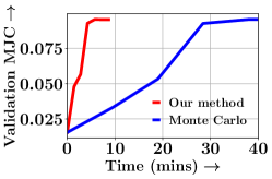
(a) Gear

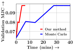
(b) Bath

Figure 9: Variation of MJC as training progresses, for Gear and Bath categories. Our proposed permutation adversarial subset selection is atleast $4\times$ faster than the Monte Carlo sampling method [79].

References

- Bach [2011] Francis Bach. Learning with submodular functions: A convex optimization perspective. arXiv preprint arXiv:1111.6453, 2011.
- Badanidiyuru et al. [2014] Ashwinkumar Badanidiyuru, Baharan Mirzasoleiman, Amin Karbasi, and Andreas Krause. Streaming submodular maximization: Massive data summarization on the fly. In Proceedings of the 20th ACM SIGKDD international conference on Knowledge discovery and data mining, pages 671–680, 2014.
- Bai et al. [2018] Wenruo Bai, William S Noble, and Jeff A Bilmes. Submodular maximization via gradient ascent: the case of deep submodular functions. Advances in neural information processing systems, 2018:7989, 2018.
- Bairi et al. [2015] Ramakrishna Bairi, Rishabh Iyer, Ganesh Ramakrishnan, and Jeff Bilmes. Summarization of multi-document topic hierarchies using submodular mixtures. In ACL, pages 553–563, 2015.
- Balcan and Harvey [2010] Maria-Florina Balcan and Nicholas JA Harvey. Submodular functions: Learnability, structure, and optimization. arXiv preprint arXiv:1008.2159, 2010.
- Balcan and Harvey [2011] Maria-Florina Balcan and Nicholas JA Harvey. Learning submodular functions. In Proceedings of the forty-third annual ACM symposium on Theory of computing, pages 793–802, 2011.
- Bilmes and Bai [2017] Jeffrey Bilmes and Wenruo Bai. Deep submodular functions. arXiv preprint arXiv:1701.08939, 2017.
- Borodin [2009] Alexei Borodin. Determinantal point processes. arXiv preprint arXiv:0911.1153, 2009.
- Cuturi [2013] Marco Cuturi. Sinkhorn distances: Lightspeed computation of optimal transport. Advances in neural information processing systems, 26:2292–2300, 2013.
- Dasgupta et al. [2013] Anirban Dasgupta, Ravi Kumar, and Sujith Ravi. Summarization through submodularity and dispersion. In Proceedings of the 51st Annual Meeting of the Association for Computational Linguistics (Volume 1: Long Papers), pages 1014–1022, 2013.
- De et al. [2016] Abir De, Isabel Valera, Niloy Ganguly, Sourangshu Bhattacharya, and Manuel Gomez Rodriguez. Learning and forecasting opinion dynamics in social networks. Advances in neural information processing systems, 29, 2016.
- De et al. [2018a] Abir De, Sourangshu Bhattacharya, and Niloy Ganguly. Demarcating endogenous and exogenous opinion diffusion process on social networks. In Proceedings of the 2018 World Wide Web Conference, pages 549–558, 2018a.
- De et al. [2018b] Abir De, Sourangshu Bhattacharya, and Niloy Ganguly. Shaping opinion dynamics in social networks. In Proceedings of the 17th international conference on autonomous agents and multiagent systems, pages 1336–1344, 2018b.
- De et al. [2019] Abir De, Sourangshu Bhattacharya, Parantapa Bhattacharya, Niloy Ganguly, and Soumen Chakrabarti. Learning linear influence models in social networks from transient opinion dynamics. ACM Transactions on the Web (TWEB), 13(3):1–33, 2019.
- De et al. [2020] Abir De, Paramita Koley, Niloy Ganguly, and Manuel Gomez-Rodriguez. Regression under human assistance. AAAI, 2020.
- De et al. [2021] Abir De, Nastaran Okati, Ali Zarezade, and Manuel Gomez-Rodriguez. Classification under human assistance. AAAI, 2021.
- [17] Indradyumna Roy Soumen Chakrabarti Abir De. Maximum common subgraph guided graph retrieval: Late and early interaction networks.
- Devlin et al. [2018] Jacob Devlin, Ming-Wei Chang, Kenton Lee, and Kristina Toutanova. Bert: Pre-training of deep bidirectional transformers for language understanding. arXiv preprint arXiv:1810.04805, 2018.
- Du et al. [2012] Donglei Du, Ruixing Lu, and Dachuan Xu. A primal-dual approximation algorithm for the facility location problem with submodular penalties. Algorithmica, 63(1):191–200, 2012.
- Durga et al. [2021] S Durga, Rishabh Iyer, Ganesh Ramakrishnan, and Abir De. Training data subset selection for regression with controlled generalization error. In International Conference on Machine Learning, pages 9202–9212. PMLR, 2021.
- El Halabi and Jegelka [2020] Marwa El Halabi and Stefanie Jegelka. Optimal approximation for unconstrained non-submodular minimization. In International Conference on Machine Learning, pages 3961–3972. PMLR, 2020.
- Elenberg et al. [2016] Ethan R Elenberg, Rajiv Khanna, Alexandros G Dimakis, and Sahand Negahban. Restricted strong convexity implies weak submodularity. arXiv preprint arXiv:1612.00804, 2016.
- Feldman and Vondrák [2016] Vitaly Feldman and Jan Vondrák. Optimal bounds on approximation of submodular and xos functions by juntas. SIAM Journal on Computing, 45(3):1129–1170, 2016.
- Flanders [1973] Harley Flanders. Differentiation under the integral sign. The American Mathematical Monthly, 80(6):615–627, 1973.
- Frieze [1974] Alan M Frieze. A cost function property for plant location problems. Mathematical Programming, 7(1):245–248, 1974.
- Fujishige [2005] Satoru Fujishige. Submodular functions and optimization. Elsevier, 2005.
- Fujishige and Iwata [1999] Satoru Fujishige and Satoru Iwata. Minimizing a submodular function arising from a concave function. Discrete applied mathematics, 92(2-3):211–215, 1999.
- Ghadiri et al. [2020] Mehrdad Ghadiri, Richard Santiago, and Bruce Shepherd. A parameterized family of meta-submodular functions. arXiv preprint arXiv:2006.13754, 2020.
- Ghadiri et al. [2021] Mehrdad Ghadiri, Richard Santiago, and Bruce Shepherd. Beyond submodular maximization via one-sided smoothness. In Proceedings of the 2021 ACM-SIAM Symposium on Discrete Algorithms (SODA), pages 1006–1025. SIAM, 2021.
- Gillenwater et al. [2014] Jennifer A Gillenwater, Alex Kulesza, Emily Fox, and Ben Taskar. Expectation-maximization for learning determinantal point processes. Advances in Neural Information Processing Systems, 27:3149–3157, 2014.
- Goemans et al. [2009] Michel X Goemans, Nicholas JA Harvey, Satoru Iwata, and Vahab Mirrokni. Approximating submodular functions everywhere. In Proceedings of the twentieth annual ACM-SIAM symposium on Discrete algorithms, pages 535–544. SIAM, 2009.
- Gupta et al. [2021] Akhil Gupta, Lavanya Marla, Ruoyu Sun, Naman Shukla, and Arinbjörn Kolbeinsson. Pender: Incorporating shape constraints via penalized derivatives. In AAAI, 2021. URL https://www.aaai.org/AAAI21Papers/AAAI-9099.GuptaA.pdf.
- Gupta et al. [2020] Maya R. Gupta, Erez Louidor Ilan, Olexander Mangylov, Nobuyuki Morioka, Taman Narayan, and Sen Zhao. Multidimensional shape constraints. In ICML, 2020. URL http://proceedings.mlr.press/v119/gupta20b/gupta20b.pdf.
- Hamilton et al. [2017] Will Hamilton, Zhitao Ying, and Jure Leskovec. Inductive representation learning on large graphs. In Advances in neural information processing systems, pages 1024–1034, 2017.
- Hashemi et al. [2019] Abolfazl Hashemi, Mahsa Ghasemi, Haris Vikalo, and Ufuk Topcu. Submodular observation selection and information gathering for quadratic models. arXiv preprint arXiv:1905.09919, 2019.
- Hornik et al. [1989] Kurt Hornik, Maxwell Stinchcombe, and Halbert White. Multilayer feedforward networks are universal approximators. Neural networks, 2(5):359–366, 1989.
- Iyer et al. [2021] Rishabh Iyer, Ninad Khargoankar, Jeff Bilmes, and Himanshu Asanani. Submodular combinatorial information measures with applications in machine learning. In Algorithmic Learning Theory, pages 722–754. PMLR, 2021.
- Jaccard [1901] Paul Jaccard. ’E comparative study of floral distribution in a portion of the alps and jura. Bull Soc Vaudoise Sci Nat, 37:547–579, 1901.
- Jegelka and Bilmes [2009] Stefanie Jegelka and Jeff Bilmes. Notes on graph cuts with submodular edge weights. In NIPS 2009 Workshop on Discrete Optimization in Machine Learning: Submodularity, Sparsity Polyhedra (DISCML), pages 1–6, 2009.
- Jegelka and Bilmes [2010] Stefanie Jegelka and Jeff Bilmes. Cooperative cuts: Graph cuts with submodular edge weights. 2010.
- Jegelka and Bilmes [2011] Stefanie Jegelka and Jeff Bilmes. Submodularity beyond submodular energies: coupling edges in graph cuts. In CVPR 2011, pages 1897–1904. IEEE, 2011.
- Karalias et al. [2021] Nikolaos Karalias, Joshua David Robinson, Andreas Loukas, and Stefanie Jegelka. Neural extensions: Training neural networks with set functions. 2021.
- Kempe et al. [2003] David Kempe, Jon Kleinberg, and Éva Tardos. Maximizing the spread of influence through a social network. In Proceedings of the ninth ACM SIGKDD international conference on Knowledge discovery and data mining, pages 137–146, 2003.
- Khanna et al. [2017] Rajiv Khanna, Ethan Elenberg, Alexandros G Dimakis, Sahand Negahban, and Joydeep Ghosh. Scalable greedy feature selection via weak submodularity. arXiv preprint arXiv:1703.02723, 2017.
- Killamsetty et al. [2021a] Krishnateja Killamsetty, Durga Sivasubramanian, Baharan Mirzasoleiman, Ganesh Ramakrishnan, Abir De, and Rishabh Iyer. Grad-match: A gradient matching based data subset selection for efficient learning. arXiv preprint arXiv:2103.00123, 2021a.
- Killamsetty et al. [2021b] Krishnateja Killamsetty, Durga Subramanian, Ganesh Ramakrishnan, and Rishabh Iyer. Glister: A generalization based data selection framework for efficient and robust learning. In AAAI, 2021b.
- Kipf and Welling [2016] Thomas N Kipf and Max Welling. Semi-supervised classification with graph convolutional networks. arXiv preprint arXiv:1609.02907, 2016.
- Kobyzev et al. [2021] Ivan Kobyzev, Simon Prince, and Marcus A. Brubaker. Normalizing flows: An introduction and review of current methods. IEEE Transactions on Pattern Analysis and Machine Intelligence, 43:3964–3979, 2021. URL http://arxiv.org/pdf/1908.09257.
- Koley et al. [2021] Paramita Koley, Avirup Saha, Sourangshu Bhattacharya, Niloy Ganguly, and Abir De. Demarcating endogenous and exogenous opinion dynamics: An experimental design approach. arXiv preprint arXiv:2102.05954, 2021.
- Kothawade et al. [2020] Suraj Kothawade, Jiten Girdhar, Chandrashekhar Lavania, and Rishabh Iyer. Deep submodular networks for extractive data summarization. arXiv preprint arXiv:2010.08593, 2020.
- Lee et al. [2019] Juho Lee, Yoonho Lee, Jungtaek Kim, Adam Kosiorek, Seungjin Choi, and Yee Whye Teh. Set transformer: A framework for attention-based permutation-invariant neural networks. In ICML, 2019.
- Lin and Bilmes [2011] Hui Lin and Jeff Bilmes. A class of submodular functions for document summarization. In Proceedings of the 49th annual meeting of the association for computational linguistics: human language technologies, pages 510–520, 2011.
- Lin and Bilmes [2012] Hui Lin and Jeff A Bilmes. Learning mixtures of submodular shells with application to document summarization. arXiv preprint arXiv:1210.4871, 2012.
- Lovász [1983] László Lovász. Submodular functions and convexity. In Mathematical programming the state of the art, pages 235–257. Springer, 1983.
- Lu et al. [2017] Zhou Lu, Hongming Pu, Feicheng Wang, Zhiqiang Hu, and Liwei Wang. The expressive power of neural networks: A view from the width. Advances in neural information processing systems, 30, 2017.
- Manupriya et al. [2022] Piyushi Manupriya, Tarun Ram Menta, Sakethanath N. Jagarlapudi, and Vineeth N. Balasubramanian. Improving attribution methods by learning submodular functions. In Gustau Camps-Valls, Francisco J. R. Ruiz, and Isabel Valera, editors, Proceedings of The 25th International Conference on Artificial Intelligence and Statistics, volume 151 of Proceedings of Machine Learning Research, pages 2173–2190. PMLR, 28–30 Mar 2022. URL https://proceedings.mlr.press/v151/manupriya22a.html.
- Mena et al. [2018] Gonzalo Mena, David Belanger, Scott Linderman, and Jasper Snoek. Learning latent permutations with gumbel-sinkhorn networks. arXiv preprint arXiv:1802.08665, 2018.
- Mirchandani and Francis [1990] Pitu B Mirchandani and Richard L Francis. Discrete location theory. 1990.
- Nemhauser et al. [1978] George L Nemhauser, Laurence A Wolsey, and Marshall L Fisher. An analysis of approximations for maximizing submodular set functions—i. Mathematical programming, 14(1):265–294, 1978.
- Okati et al. [2021] Nastaran Okati, Abir De, and Manuel Rodriguez. Differentiable learning under triage. Advances in Neural Information Processing Systems, 34:9140–9151, 2021.
- Ortiz-Astorquiza et al. [2015] Camilo Ortiz-Astorquiza, Ivan Contreras, and Gilbert Laporte. Multi-level facility location as the maximization of a submodular set function. European Journal of Operational Research, 247(3):1013–1016, 2015.
- Pabbaraju and Jain [2019] Chirag Pabbaraju and Prateek Jain. Learning functions over sets via permutation adversarial networks. arXiv preprint arXiv:1907.05638, 2019. URL https://arxiv.org/pdf/1907.05638.
- Powers et al. [2018] Thomas Powers, Rasool Fakoor, Siamak Shakeri, Abhinav Sethy, Amanjit Kainth, Abdel-rahman Mohamed, and Ruhi Sarikaya. Differentiable greedy networks. arXiv preprint arXiv:1810.12464, 2018.
- Qi et al. [2017] Charles R Qi, Hao Su, Kaichun Mo, and Leonidas J Guibas. Pointnet: Deep learning on point sets for 3d classification and segmentation. In Proceedings of the IEEE conference on computer vision and pattern recognition, pages 652–660, 2017.
- Ravanbakhsh et al. [2016] Siamak Ravanbakhsh, Jeff Schneider, and Barnabas Poczos. Deep learning with sets and point clouds. arXiv preprint arXiv:1611.04500, 2016.
- Ren et al. [2018] Mengye Ren, Wenyuan Zeng, Bin Yang, and Raquel Urtasun. Learning to reweight examples for robust deep learning. In International Conference on Machine Learning, pages 4334–4343, 2018.
- Rezatofighi et al. [2020] Hamid Rezatofighi, Roman Kaskman, Farbod T Motlagh, Qinfeng Shi, Anton Milan, Daniel Cremers, Laura Leal-Taixé, and Ian Reid. Learn to predict sets using feed-forward neural networks. arXiv preprint arXiv:2001.11845, 2020.
- Roy et al. [2021] Indradyumna Roy, Abir De, and Soumen Chakrabarti. Adversarial permutation guided node representations for link prediction. In arXiv:2012.08974, 2021.
- Roy et al. [2022] Indradyumna Roy, Venkata Sai Baba Reddy Velugoti, Soumen Chakrabarti, and Abir De. Interpretable neural subgraph matching for graph retrieval. In Proceedings of the AAAI Conference on Artificial Intelligence, volume 36, pages 8115–8123, 2022.
- Sakaue [2021] Shinsaku Sakaue. Differentiable greedy algorithm for monotone submodular maximization: Guarantees, gradient estimators, and applications. In International Conference on Artificial Intelligence and Statistics, pages 28–36. PMLR, 2021.
- Samanta et al. [2020] Bidisha Samanta, Abir De, Gourhari Jana, Vicenç Gómez, Pratim Kumar Chattaraj, Niloy Ganguly, and Manuel Gomez-Rodriguez. Nevae: A deep generative model for molecular graphs. Journal of machine learning research. 2020 Apr; 21 (114): 1-33, 2020.
- Schrijver [2003] Alexander Schrijver. Combinatorial optimization: polyhedra and efficiency, volume 24. Springer Science & Business Media, 2003.
- Shamaiah et al. [2010] Manohar Shamaiah, Siddhartha Banerjee, and Haris Vikalo. Greedy sensor selection: Leveraging submodularity. In 49th IEEE conference on decision and control (CDC), pages 2572–2577. IEEE, 2010.
- Singla et al. [2016] Adish Singla, Sebastian Tschiatschek, and Andreas Krause. Noisy submodular maximization via adaptive sampling with applications to crowdsourced image collection summarization. In AAAI, 2016.
- Sipos et al. [2012] Ruben Sipos, Pannaga Shivaswamy, and Thorsten Joachims. Large-margin learning of submodular summarization models. In Proceedings of the 13th Conference of the European Chapter of the Association for Computational Linguistics, pages 224–233, 2012.
- Stobbe and Krause [2010] Peter Stobbe and Andreas Krause. Efficient minimization of decomposable submodular functions. arXiv preprint arXiv:1010.5511, 2010.
- Tschiatschek et al. [2014] Sebastian Tschiatschek, Rishabh K Iyer, Haochen Wei, and Jeff A Bilmes. Learning mixtures of submodular functions for image collection summarization. In Advances in neural information processing systems, pages 1413–1421, 2014.
- Tschiatschek et al. [2016] Sebastian Tschiatschek, Josip Djolonga, and Andreas Krause. Learning probabilistic submodular diversity models via noise contrastive estimation. In Artificial Intelligence and Statistics, pages 770–779. PMLR, 2016.
- Tschiatschek et al. [2018] Sebastian Tschiatschek, Aytunc Sahin, and Andreas Krause. Differentiable submodular maximization. arXiv preprint arXiv:1803.01785, 2018.
- Verma et al. [2022] Tathagat Verma, Abir De, Yateesh Agrawal, Vishwa Vinay, and Soumen Chakrabarti. Varscene: A deep generative model for realistic scene graph synthesis. In International Conference on Machine Learning, pages 22168–22183. PMLR, 2022.
- [81] Jan Vondrák. Submodularity and curvature: the optimal algorithm.
- Wagstaff et al. [2019] Edward Wagstaff, Fabian Fuchs, Martin Engelcke, Ingmar Posner, and Michael A. Osborne. On the limitations of representing functions on sets. In Proceedings of the 36th International Conference on Machine Learning, 2019.
- Wehenkel and Louppe [2019] Antoine Wehenkel and Gilles Louppe. Unconstrained monotonic neural networks. NeurIPS, 2019.
- Wei et al. [2015] Kai Wei, Rishabh Iyer, and Jeff Bilmes. Submodularity in data subset selection and active learning. In International Conference on Machine Learning, pages 1954–1963, 2015.
- Yu and Blaschko [2015] Jiaqian Yu and Matthew Blaschko. Learning submodular losses with the lovász hinge. In International Conference on Machine Learning, pages 1623–1631. PMLR, 2015.
- Zaheer et al. [2017] Manzil Zaheer, Satwik Kottur, Siamak Ravanbakhsh, Barnabas Poczos, Ruslan Salakhutdinov, and Alexander Smola. Deep sets. arXiv preprint arXiv:1703.06114, 2017.
- Zarezade et al. [2017] Ali Zarezade, Abir De, Hamid Rabiee, and Manuel Gomez Rodriguez. Cheshire: An online algorithm for activity maximization in social networks. arXiv preprint arXiv:1703.02059, 2017.
- Zhang and Vorobeychik [2016] Haifeng Zhang and Yevgeniy Vorobeychik. Submodular optimization with routing constraints. In Proceedings of the AAAI conference on artificial intelligence, volume 30, 2016.
- Zhang et al. [2021] Ping Zhang, Rishabh Iyer, Ashish Tendulkar, Gaurav Aggarwal, and Abir De. Learning to select exogenous events for marked temporal point process. Advances in Neural Information Processing Systems, 34:347–361, 2021.
- Zhang et al. [2019] Yan Zhang, Jonathon Hare, and Adam Prugel-Bennett. Deep set prediction networks. Advances in Neural Information Processing Systems, 32:3212–3222, 2019.
- Zhang and Sabuncu [2018] Zhilu Zhang and Mert Sabuncu. Generalized cross entropy loss for training deep neural networks with noisy labels. In Advances in neural information processing systems, pages 8778–8788, 2018.