Maximum Common Subgraph Guided Graph Retrieval:
Late and Early Interaction Networks

Abstract

The graph retrieval problem is to search in a large corpus of graphs for ones that are most similar to a query graph. A common consideration for scoring similarity is the maximum common subgraph (MCS) between the query and corpus graphs, usually counting the number of common edges (i.e., MCES). In some applications, it is also desirable that the common subgraph be connected, i.e., the maximum common connected subgraph (MCCS). Finding exact MCES and MCCS is intractable, but may be unnecessary if ranking corpus graphs by relevance is the goal. We design fast and trainable neural functions that approximate MCES and MCCS well. Late interaction methods compute representations for the query and corpus graphs separately, and compare these representations using simple similarity functions at the last stage, leading to highly scalable systems. Early interaction methods combine information from both graphs right from the input stages, are usually considerably more accurate, but slower. We propose both late and early interaction neural MCES and MCCS formulations. They are both based on a continuous relaxation of a node alignment matrix between query and corpus nodes. For MCCS, we propose a novel differentiable ‘gossip’ network for estimating the size of the largest connected common subgraph. Extensive experiments with seven data sets show that our proposals are superior among late interaction models in terms of both accuracy and speed. Our early interaction models provide accuracy competitive with the state of the art, at substantially greater speeds.

1 Introduction

Given a query graph, the graph retrieval problem is to search for relevant or similar response graphs from a corpus of graphs [1, 2, 3, 4, 5, 6, 7, 8, 9, 10, 11, 12]. Depending on the application, the notion of relevance may involve graph edit distance (GED) [13, 14, 15], the size of the maximum common subgraph (MCS) [6, 7, 8, 9, 10], full graph or subgraph isomorphism [6, 11, 12], etc. In this work, we focus on two variations of MCS-based relevance measures: (i) maximum common edge subgraph (MCES) [16], which has applications in distributed computing [17, 16] and molecule search [18, 19, 20, 21] and (ii) maximum common connected subgraph (MCCS) [22], which has applications in keyword search over knowledge graphs [23, 24], software development [25, 26, 27], image analysis [28, 29, 30], etc.

In recent years, there has been an increasing interest in designing neural graph retrieval models [6, 7, 8, 9, 10, 11]. However, most of them learn black box relevance models which provide suboptimal performance in the context of MCS based retrieval (Section 4). Moreover, they do not provide intermediate matching evidence to justify their scores and therefore, they lack interpretability. In this context, Li et al. [6] proposed a graph matching network (GMN) [6] based on a cross-graph attention mechanism, which works extremely well in practice (Section 4). Nevertheless, it suffers from three key limitations, leaving considerable scope for the design of enhanced retrieval models. (i) Similar to other graph retrieval models, it uses a general-purpose scoring layer, which renders it suboptimal in the context of MCS based graph retrieval. (ii) As acknowledged by the authors, GMN is slow in both training and inference, due to the presence of the expensive cross-attention mechanism. (iii) MCS or any graph similarity function entails an injective mapping between nodes and edges across the graph pairs. In contrast, cross-attention induces potentially inconsistent and non-injective mappings, where a given query node can be mapped to multiple corpus nodes and vice-versa.

1.1 Our contributions

We begin by writing down (the combinatorial forms of) MCES and MCCS objectives in specific ways that facilitate subsequent adaptation to neural optimization using both late and early interaction networks. Notably, these networks are trained end-to-end, using only the distant supervision by MCES or MCCS values of query-corpus graph pairs, without explicit annotation of the structural mappings identifying the underlying common subgraph.

Late interaction models. We use a graph neural network (GNN) to first compute the node embeddings of the query and corpus graphs independently of each other and then deploy an interaction network for computing the relevance scores. This decoupling between embedding computation and interaction steps leads to efficient training and inference. We introduce LMCES and LMCCS, two late interaction neural architectures for MCES and MCCS based graph retrieval respectively. The interaction model is a differentiable graph alignment planner. It learns a Gumbel-Sinkhorn (GS) network to provide an approximate alignment plan between the query and corpus graphs. In contrast to GMN [6], it induces an approximately injective mapping between the nodes and edges of the query and corpus graphs. The MCES objective is then computed as a differentiable network applied to this mapping. For MCCS, we further develop a novel differentiable gossip network that computes the size of the largest connected component in the common subgraph estimated from the above mapping. These neural gadgets may be of independent interest.

Early interaction model. In the early interaction model, we perform the interaction step during the node embedding computation phase, which makes the query and corpus embeddings dependent on each other. This improves predictive power, at the cost of additional training and inference time. Here, we propose XMCS (cross-MCS), an early interaction model that works well for both MCES and MCCS based graph retrieval. At each propagation layer of the GNN, we first refine the alignment plan using the embeddings computed in the previous layer, then update the underlying coverage objective using the refined alignment and finally use these signals to compute the node embeddings of the current layer.

Comprehensive evaluation. We experiment with seven diverse datasets, which show that: (i) our late and early interaction models outperform the corresponding state-of-the-art methods in terms of both accuracy and inference time; (ii) in many cases, LMCES and LMCCS outperform the early interaction model of GMN [6]; and (iii) GMN’s accuracy can be significantly improved by substituting its final layer with our MCS-specific neural surrogate.

1.2 Related work

Combinatorial algorithms for MCS. Both MCES and MCCS are NP-complete [16]. Several works designed heuristics for computing MCES for specific types of graphs [19, 18, 31]. Bahiense et al. [16] formulated MCES as an integer programming problem, provided a polyhedral analysis of the underlying formulation, and finally designed a branch and cut algorithm to solve it. Such polyhedral study for MCES was also performed by others [32, 33]. Combinatorial methods for different variants of MCCS have also been thoroughly studied. Some of them provide exact MCCS [34, 35, 36]. McCreesh et al. [34] proposed McSplit, a branch and bound algorithm for maximum common induced and connected graph, which is efficient in terms of time and memory. Other works provide effective heuristics to find approximate MCCS [37, 38]. However, these methods are not differentiable and therefore not suitable for data-driven MCS estimation.

Learning models for MCS. There are some recent efforts to design machine learning models for graph similarity and search [39, 8]. Among them, Bai et al. [39, GLsearch] compute MCS between two graphs using a reinforcement learning setup. In contrast, we consider a supervised learning setting for graph retrieval. Although Bai et al. [8, GraphSim] focus on the supervised learning scenario, their relevance scoring model performs poorly for MCS based retrieval.

Graph matching for computer vision. Neural models for graph matching are used in applications of computer vision for computing image similarity, object detection, etc. However, these applications permit explicit supervision of the underlying node alignments [40, 41, 42, 43, 44, 45, 46, 47, 48, 49]. They adopt different types of losses which include permutation loss [42, 43, 44, 45], Hungarian loss [47], and displacement loss [41]. In our problem, we only use distant supervision in the form of size of the underlying MCS. Moreover, these work mostly consider graph matching problems, whereas we consider maximum common subgraph detection using distant supervision from MCS score alone.

Graph representation learning. Representation learning on graphs has been widely researched in the last decade [50, 51, 52, 53, 54, 55]. Among them, graph neural networks (GNN) are the most popular node embedding models [50, 51, 52, 53, 56, 57]. Given a node $u$, a GNN collects information from $K$-hop neighbors of the node $u$ and applies a symmetric aggregator on top of it to obtain the representation vector of the nodes. In the context of graph retrieval, the node embeddings are used in two ways. In the first approach, they are further aggregated into graph embeddings, which are then used to compute the similarity between query and corpus graphs, by comparing the embeddings in the vector space [11, 6]. The second approach consists of SimGNN [7], GOTSim [9], GraphSim [8], GEN [6] and GMN [6], which compare the node embeddings and find suitable alignments between them. Here, GMN applies cross attention based mechanism on the node embeddings given a graph neural network [50]. Recently, Chen et al. [58] designed a structure aware transformer architecture, which can represent a subgraph around a node more effectively than several other representation models.

Differentiable solvers for combinatorial algorithms. Our work attempts to find a neural surrogate for the combinatorial challenge of maximizing objective scores over a permutation space. In effect, we are attempting to solve an Optimal Transport problem, where the central challenge is to present a neural gadget which is differentiable and backpropagable, thus enabling end-to-end training. Cuturi [59] utilized iterative row and column normalization, earlier proposed by Sinkhorn [60], to approximately solve the transportation problem subject to marginal constraints. In another approach, Vlastelica et al. [61] attempted to solve combinatorial problems exactly using available black-box solvers, by proposing to use the derivative of an affine surrogate of the piece-wise constant function in the backward pass. Rolínek et al. [62] leverage this to perform deep graph matching based on explicit supervision of the ground truth node alignments. In another approach, Berthet et al. [63] perturb the inputs to the discrete solvers with random noise, so as to make them differentiable. Karalias and Loukas [64] design probabilistic loss functions for tackling the combinatorial objective of selecting a subset of nodes adhering to some given property. Finally, Kotary et al. [65] present a detailed survey of the existing neural approaches for solving constrained optimization problems on graphs.

2 Late interaction models for MCES and MCCS

In this section, we first write down the exact objectives for MCES and MCCS. These expressions are partly based upon a pairing of nodes between query and corpus graphs, and partly on typical graph algorithms. They lead naturally to our subsequent development of two late interaction models, LMCES and LMCCS. We begin with formal definitions of MCES and MCCS.

Definition 1 (MCES and MCCS)

Given query and corpus graphs $G_{q}{=}(V_{q},E_{q})$ and $G_{c}{=}(V_{c},E_{c})$.

1. The maximum common edge subgraph $\operatorname{MCES}(G_{q},G_{c})$ is the common (not necessarily induced nor connected) subgraph between $G_{q}$ and $G_{c}$, having the maximum number of edges [16].

2. The maximum common connected subgraph $\operatorname{MCCS}(G_{q},G_{c})$ is the common connected subgraph with the maximum number of nodes [22].

2.1 Combinatorial formulations for MCES and MCCS

As mentioned in Section 1.2, combinatorial algorithms for MCES and MCCS abound in the literature [35, 34, 16, 19, 18, 31]. However, it is difficult to design neural surrogates for these algorithms. Therefore, we come up with the new optimization objectives for MCES and MCCS, which allow us to design neural surrogates by gradually replacing its different components with differentiable parameterized components.

Exact MCES. Given a query graph $G_{q}=(V_{q},E_{q})$ and a corpus graph $G_{c}=(V_{c},E_{c})$, we pad the graph having fewer vertices (typically, $G_{q}$), with $||V_{c}|-|V_{q}||$ disconnected nodes. This ensures that the padded graphs have an equal number of nodes $N$. Let us denote the adjacency matrices of $G_{q}$ and $G_{c}$ (after padding) as $\bm{A}_{q}\in\{0,1\}^{N\times N}$ and $\bm{A}_{c}\in\{0,1\}^{N\times N}$. To find $\operatorname{MCES}(G_{q},G_{c})$ from the adjacency matrices $\bm{A}_{q}$ and $\bm{A}_{c}$, we first obtain the candidate common subgraph under some proposed node alignment given by permutations ${\bm{P}}$ of $\bm{A}_{c}$, which can be characterized by the adjacency matrix $\min(\bm{A}_{q},{\bm{P}}\bm{A}_{c}{\bm{P}}^{T})$. This matrix shows the overlapping edges under the proposed node alignment. Subsequently, we choose the permutation which maximizes the total number of edges in this subgraph. Formally, we compute the MCES score by solving a coverage maximization problem, as follows:

$$\textstyle\max_{{\bm{P}}\in\mathcal{P}}\ \sum_{i,j}\min\big{(}\bm{A}_{q},{\bm{P}}\bm{A}_{c}{\bm{P}}^{\top}\big{)}_{i,j}$$ (1)

where $\mathcal{P}$ is the set of permutation matrices of size $N\times N$ and the $\min$ operator is applied elementwise.

Exact MCCS. MCES does not require the common subgraph to be connected, which may be desirable in some applications. For example, in keyword search and question answering over knowledge graphs (KGs) [23, 66, 24], one may wish to have the entity nodes, forming the response, to be connected to each other. In molecule search, one may require a connected functional group to be present in both query and corpus graphs [20]. In such situations, MCCS may be more appropriate.

Given a query graph $G_{q}$ and a corpus graph $G_{c}$ and their adjacency matrices $\bm{A}_{q}$ and $\bm{A}_{c}$ after padding, we first apply a row-column permutation on $\bm{A}_{c}$ using the permutation matrix ${\bm{P}}$ and obtain the candidate common subgraph with adjacency matrix $\min(\bm{A}_{q},{\bm{P}}\bm{A}_{c}{\bm{P}}^{\top})$. Then we apply Tarjan’s algorithm [67] to return the size of the largest connected component, which we maximize w.r.t. ${\bm{P}}$:

$$\textstyle\max_{{\bm{P}}\in\mathcal{P}}\ \textsc{TarjanSCC}\left(\min\big{(}\bm{A}_{q},{\bm{P}}\bm{A}_{c}{\bm{P}}^{\top}\big{)}\right).$$ (2)

Here TarjanSCC takes the adjacency matrix as input and returns the size of the largest connected component of corresponding graph.

Bottleneck of approximating the optimization problems (1) and (2). One way of avoiding the intractability of searching through ${\bm{P}}$, is to replace the hard permutation matrix with a differentiable soft surrogate via the Gumbel-Sinkhorn (GS) network [68, also see Section B]. However, such a relaxation is not adequate on its own.

1. Most elements of $\min(\bm{A}_{q},{\bm{P}}\bm{A}_{c}{\bm{P}}^{\top})$ are binary, which deprives the learner of gradient signals.

2. In practice, the nodes or edges may have associated (noisy) features, which play an important role in determining similarity between nodes or edges across query and corpus graphs. For example, in scene graph based image retrieval, "panther" may be deemed similar to "leopard". The objectives in Eqs. (1) and (2) do not capture such phenomenon.

3. Tarjan’s algorithm first applies DFS on a graph to find the connected components and then computes the size of the largest among them, in terms of the number of nodes. Therefore, even for a fixed ${\bm{P}}$, it is not differentiable.

Next, we address the above bottlenecks by replacing the objectives (1) and (2) with two neural surrogates, which are summarized in Figure 1.

2.2 Design of LMCES

We design the neural surrogate of Eq. (1) by replacing the adjacency matrices with the corresponding continuous node embeddings computed by a GNN, and the hard permutation matrix with a soft surrogate—a doubly stochastic matrix—generated by the Gumbel-Sikhorn network [68]. These node embeddings allow us to compute non-zero gradients and approximate similarity between nodes and their local neighborhood in the continuous domain. Specifically, we compute this neural surrogate in the following two steps.

Step 1: Computing node embeddings. We use a message passing graph neural network [50, 69] ${\mathrm{GNN}}_{\theta}$ with $R$ propagation layers and trainable parameters $\theta$, to compute the node embeddings $\bm{h}_{u}(1),\ldots,\bm{h}_{u}(R)\in\mathbb{R}^{d}$, for each node $u$ in the query and corpus graphs, to which ${\mathrm{GNN}}_{\theta}$ is applied separately. Finally, we build two matrices ${\bm{H}}_{q}(r),{\bm{H}}_{c}(r)\in\mathbb{R}^{N\times d}$ for $r\in[R]$ by stacking the node embedding vectors for query and corpus graphs. Formally, we have

$${\bm{H}}_{q}(1),\ldots,{\bm{H}}_{q}(R)={\mathrm{GNN}}_{\theta}(G_{q}),\qquad{\bm{H}}_{c}(1),\ldots,{\bm{H}}_{c}(R)={\mathrm{GNN}}_{\theta}(G_{c})$$ (3)

Step 2: Interaction between ${\bm{H}}_{q}(r)$ and ${\bm{H}}_{c}(r)$. In principle, the embeddings $\bm{h}_{u}(1),\ldots,\bm{h}_{u}(R)$ of a node $u$ capture information about the neighborhood of $u$. Thus, we can view the set of embedding matrices $\{{\bm{H}}_{q}(r)\,|\,r\in[R]\}$ and $\{{\bm{H}}_{c}(r)\,|\,r\in[R]\}$ as a reasonable representation of the query and corpus graphs, respectively. To compute a smooth surrogate of the adjacency matrix of the common subgraph, i.e., $\min(\bm{A}_{q},{\bm{P}}\bm{A}_{c}{\bm{P}}^{\top})$, we seek to find the corresponding alignment between ${\bm{H}}_{q}(r)$ and ${\bm{H}}_{c}(r)$ using soft-permutation (doubly stochastic) matrices ${\bm{P}}^{(r)}$ generated through a Gumbel-Sikhorn network ${\mathrm{GS}}_{\phi}$. Here, we feed ${\bm{H}}_{q}(r)$ and ${\bm{H}}_{c}(r)$ into ${\mathrm{GS}}_{\phi}$ and obtain a doubly stochastic matrix ${\bm{P}}^{(r)}$:

$${\bm{P}}^{(r)}={\mathrm{GS}}_{\phi}({\bm{H}}_{q}(r),{\bm{H}}_{c}(r))\quad\forall\ r\in[R]$$ (4)

Finally, we replace the true relevance scoring function in Eq. (1) with the following smooth surrogate:

$$s(G_{q},G_{c}) =\sum_{r\in[R]}w_{r}\sum_{i,j}\min({\bm{H}}_{q}(r),{\bm{P}}^{(r)}{\bm{H}}_{c}(r))_{i,j}$$ (5)

Here $\{w_{r}\geq 0:r\in[R]\}$ are trainable parameters, balancing the quality of signals over all message rounds $r$. Note that the $R$ message rounds execute on the query and corpus graphs separately. The interaction between corresponding rounds, happens at the very end.

2.3 Design of LMCCS

In case of MCES, our key modification was to replace the adjacency matrices with node embeddings and design a differentiable network to generate a soft-permutation matrix. In the case of MCCS, we have to also replace the non-differentiable step of finding the size of the largest connected component of the common subgraph with a neural surrogate, for which we design a novel gossip protocol.

Differentiable gossip protocol to compute the largest connected component. Given any graph $G=(V,E)$ with the adjacency matrix $\bm{B}$, we can find its largest connected component (LCC) by using a gossip protocol. At iteration $t=0$, we start with assigning each node a message vector $\bm{x}_{u}(0)\in\mathbb{R}^{N}$, which is the one-hot encoding of the node $u$, i.e., $\bm{x}_{u}(0)[v]=1$ for $v=u$ and $0$ otherwise. In iteration $t>0$, we update the message vectors $\bm{x}_{u}(t+1)$ as $\textstyle\bm{x}_{u}(t+1)=\sum_{v\in\text{nbr}(u)\cup\left\{u\right\}}\bm{x}_{v}(t)$. Here, $\text{nbr}(u)$ is the set of neighbors of $u$. Initially we start with sparse vector $\bm{x}_{u}$ with exactly one non-zero entry. As we increase the number of iterations, $u$ would gradually collect messages from

Algorithm 1 Gossip($\bm{B}$)

1:$\mathbf{X}(0)=\mathbb{I}$  #  identity

2:for $t=1,\ldots T-1$ do

3:    $\mathbf{X}(t+1)\leftarrow\mathbf{X}(t)(\bm{B}+\mathbb{I})$

4:Return $\max_{u\in V}||\mathbf{X}(T)[\bullet,u]||_{0}$

the distant nodes which are reachable from $u$. This would increase the number of non-zero entries of $\bm{x}_{u}$. For sufficiently large value of iterations $T$ (diameter of $G$), we will attain $\bm{x}_{u}(T)[v]\neq 0$ whenever $u$ and $v$ lie in the same connected component and $\bm{x}_{u}(T)[v]=0$, otherwise. Once this stage is reached, one can easily compute the number of nodes in the largest connected component of $G$ as $\max_{u}||\bm{x}_{u}(T)||_{0}$, i.e., the maximum number of non-zero entries in a message vector. Algorithm 1 shows the gossip protocol, with the adjacency matrix $\bm{B}$ as input and the size of the largest connected component as output.

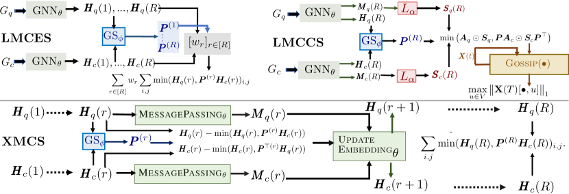
Figure 1: Proposed late (top row) and early (bottom row) interaction models. Top Left: LMCES encodes the given query-corpus graphs separately, using $R$ layers of ${\mathrm{GNN}}_{\theta}$ to compute node embedding matrices ${\bm{H}}_{q}(r),{\bm{H}}_{c}(r)$ with $r=\left\{1,\ldots,R\right\}$. For each layer $r$, the Gumbel-Sinkhorn network ${\mathrm{GS}}_{\phi}$ computes the optimal alignment ${\bm{P}}^{(r)}$ between ${\bm{H}}_{q}(r)$ and ${\bm{H}}_{c}(r)$, which is finally used compute the relevance score in Eq. (5). Top Right: LMCCS uses ${\mathrm{GNN}}_{\theta}$ to encode the $R$-hop node and edge embeddings, ${\bm{H}}_{\bullet}(R)$ and $\bm{M}_{\bullet}(R)$. The edge embeddings $\bm{M}_{\bullet}(R)$ are fed into $L_{\alpha}$ to predict edge score matrix $\bm{S}_{\bullet}(R)$ whose valid edge entries are encoded in $\bm{A}\odot\bm{S}$. As before, ${\mathrm{GS}}_{\phi}({\bm{H}}_{q}(R),{\bm{H}}_{c}(R))$ generates alignment ${\bm{P}}^{(R)}$ which is used to compute candidate MCS graph $\min(\bm{A}_{q}\odot\bm{S}_{q},{\bm{P}}(\bm{A}_{c}\odot\bm{S}_{c}){\bm{P}}^{\top})$, which is then fed into the neural Gossip module, to predict the final MCCS score. Bottom: At each layer $r$, XMCS uses the alignment matrix ${\bm{P}}^{(r)}$ to factor the cross graph influences using ${\bm{H}}_{q}(r)-\min({\bm{H}}_{q}(r),{\bm{P}}^{(r)}{\bm{H}}_{c}(r))$ for query, and ${\bm{H}}_{c}(r)-\min({\bm{H}}_{c}(r),{{\bm{P}}^{(r)}}^{T}{\bm{H}}_{q}(r))$ for corpus. This is used to update the node embeddings ${\bm{H}}_{\bullet}(r)\to{\bm{H}}_{\bullet}(r+1)$. Embeddings from the final layer are used to compute the final relevance score.

Exact MCCS computation using the gossip protocol. Given the query and corpus graphs $G_{q}$ and $G_{c}$ with their adjacency matrices $\bm{A}_{q}$ and $\bm{A}_{c}$, we can rewrite Eqn. (2) in the equivalent form

$$\max_{{\bm{P}}\in\mathcal{P}}\ \textsc{Gossip}(\min(\bm{A}_{q},{\bm{P}}\bm{A}_{c}{\bm{P}}^{\top})).$$ (6)

Recall that $\mathcal{P}$ is the set permutation matrices of size $N\times N$.

Neural surrogate. One can use a ${\mathrm{GS}}$ network to obtain a permutation matrix ${\bm{P}}$, which in principle, can support backpropagation of $\min(\bm{A}_{q},{\bm{P}}\bm{A}_{c}{\bm{P}}^{\top})$. However, as mentioned in Section 2.1 (items 1 and 2), $\bm{A}_{\bullet}$ is 0/1, and ${\bm{P}}$ often saturates, losing gradient signal for training. In response, we will design a neural surrogate for the true MCCS size given in Eq. (2), using three steps.

Step 1: Computation of edge embeddings. To tackle the above challenge, we introduce a parallel back-propagation path, in order to allow the GNNs to learn which edges are more important than others. To this end, we first use the GNNs to compute edge embedding vectors $\bm{m}_{e}(r)\in\mathbb{R}^{d_{E}}$ for edges $e\in E$, in addition to node embeddings at each propagation layer $r\in[R]$. Then, we gather the edge embeddings from the final layer $R$, into the matrices $\bm{M}_{q}(R),\bm{M}_{c}(R)\in\mathbb{R}^{|E|\times d_{E}}$ for query and corpus pairs. Next, we feed each separately into a neural network $L_{\alpha}$ with trainable parameters $\alpha$, which predicts the importance of edges based on each edge embedding. Thus, we obtain two matrices $\bm{S}_{q}\in\mathbb{R}^{N\times N}$ and $\bm{S}_{c}\in\mathbb{R}^{N\times N}$, which are composed of the edge scores between the corresponding node pairs. Formally, we have:

$${\bm{H}}_{q}(R),\bm{M}_{q}(R)={\mathrm{GNN}}_{\theta}(G_{q}),\quad {\bm{H}}_{c}(R),\bm{M}_{c}(R)={\mathrm{GNN}}_{\theta}(G_{c})$$ (7)

$$\bm{S}_{q}=L_{\alpha}\left(\bm{M}_{q}(R)\right),\quad \bm{S}_{c}=L_{\alpha}\left(\bm{M}_{c}(R)\right)$$ (8)

In our implementation, $L_{\alpha}$ consists of one linear layer, a ReLU layer and another linear layer.

Step 2: Continuous approximation of MCCS. In MCES, we approximated the MCES score in Eq. (1) directly, using the neural coverage function defined in Eq. (5) in terms of the node embeddings. Note that, here, we did not attempt to develop any continuous approximation of $\min\big{(}\bm{A}_{q},{\bm{P}}\bm{A}_{c}{\bm{P}}^{\top}\big{)}$— the adjacency matrix of the candidate common subgraph. However, in order to apply our proposed gossip protocol (or its neural approximation), we need an estimate of the adjacency matrix of the common subgraph. Therefore, we compute the noisy estimator as follows:

$${\bm{P}}={\mathrm{GS}}_{\phi}({\bm{H}}_{q}(R),{\bm{H}}_{c}(R)),\quad\ \ \bm{B}=\min\big{(}\bm{A}_{q}\odot\bm{S}_{q},{\bm{P}}(\bm{A}_{c}\odot\bm{S}_{c}){\bm{P}}^{\top}\big{)}$$ (9)

In the above expression, we replace all the non-zero entries of $\bm{A}_{q}$ and $\bm{A}_{c}$ with the corresponding edge importance scores of $\bm{S}_{q}$ and $\bm{S}_{c}$. This facilitates backpropagation more effectively, as opposed to the original 0/1 adjacency representation of the common subgraph (item 1 in Section 2.1). Here, we generate the permutation matrix ${\bm{P}}$ using Gumbel-Sinkhorn network similar to MCES, except that here we generate only one permutation matrix based on the embeddings on the final layer, whereas in MCES, we generated permutations ${\bm{P}}^{(r)}$ for each layer $r$.

Step 3: Neural implementation of gossip. Our gossip protocol in Algorithm 1 is already differentiable. However, by the virtue of the way it is designed, it would give accurate results only if the input matrix consists of 0/1 values. However, our neural estimate $\bm{B}$ contains mostly non-zero continuous values and many of them can go beyond $\pm 1$. As a result, the resultant matrix $\mathbf{X}(t)=\mathbf{X}(0)(\bm{B}+\mathbb{I})^{t}$ in Algorithm 1 may suffer from extremely poor conditioning. To tackle this problem, we use a noise filter network at the final step $T$. We first estimate a dynamic threshold $\tau\in[0,\infty)$ and then set the values of $\mathbf{X}(T)$ below that threshold to zero. Finally, we scale the non-zero entries between $(0,1)$ using a sigmoid activation $\sigma(\cdot)$. Formally, we define:

$$\tau=\textsc{Thresh}_{\beta}(\mathbf{X}(T));\qquad\mathbf{\hat{X}}(T)=2\sigma\left(\operatorname{ReLU}[\mathbf{X}(T)-\tau]/\lambda\right)-1,$$ (10)

where $\lambda$ is a temperature hyperparameter. $\textsc{Thresh}_{\beta}$ consists of a linear, a ReLU, then another linear layer. Note that $\mathbf{\hat{X}}(T)\in[0,1]$ by design, which lets us replace the $L_{0}$ norm in the final score (Algorithm 1, line 4) with the more benign $L_{1}$ norm, followed by a maxpool over nodes:

$$s(G_{q},G_{c})=\max_{u\in V}\big{\|}{\mathbf{\hat{X}}(T)}[\bullet,u]\big{\|}_{1}$$ (11)

Note that the interaction steps 2 and 3 above are completely decoupled from step 1 and do not have any contribution in computing embeddings.

3 Early/cross interaction model: XMCS

Although late interaction models offer efficient training and fast inference, prior work [6] suggests that early interaction models, while slower, may offer better accuracy. Motivated by such successes, we propose a unified early interaction model, called XMCS, which works for both MCES and MCCS. XMCS  is slower than LMCES and LMCCS, but provides significant accuracy gains (Section 4). Moreover, it is significantly faster than GMN [6]. As before, the relevance score $s(G_{q},G_{c})$ is computed using a graph neural network (GNN) with $R$ propagation layers, but each graph influences embeddings of the other graph in each layer.

Initialization of node embeddings. We start with the raw node features $\bm{z}_{u}$ for each node $u\in V_{q}\cup V_{c}$ and use them to initialize the node embeddings $\bm{h}_{u}$.

$$\bm{h}_{u}(0)=\textsc{FeatureEncoder}_{\theta}{\text{}}(\bm{z}_{u})$$ (12)

Embedding computation via interaction between $G_{q}$ and $G_{c}$. Given the node embeddings $\bm{h}_{u}(r)$ for some propagation layer $r<R$, we first encode the intra-graph influences across all edges in both query and corpus graphs. Accordingly, we obtain directed message vectors, for each pair of nodes $(u,v)\in E_{q}\cup E_{c}$, which are then aggregated using a simple sum aggregator.

$$\bm{m}_{uv}(r) =\textsc{MessagePassing}_{\theta}(\bm{h}_{u}(r),\bm{h}_{v}(r))\quad\forall\ (u,v)\in E_{q}\cup E_{c}$$ (13)

$$\overline{\bm{m}}_{u}(r) =\textstyle\sum_{v\in\text{nbr}(u)}\bm{m}_{uv}(r)\quad\forall u\in V_{q}\cup V_{c}$$ (14)

Next, we perform the interaction step across the query and corpus graphs $G_{q}$ and $G_{c}$, using a graph alignment network, which is modeled using ${\mathrm{GS}}_{\phi}$, similar to the late interaction models in Eq. (4). We build embedding matrices ${\bm{H}}_{q}(r)$ and ${\bm{H}}_{c}(r)$ by stacking $\bm{h}_{u}(r)$ from $G_{q}$ and $G_{c}$ respectively. Then, we feed them into ${\mathrm{GS}}_{\phi}$ to generate an alignment matrix, and finally compute the difference of the query and the corpus graphs from the underlying MCS in the continuous embedding space:

$${\bm{P}}^{(r)}={\mathrm{GS}}_{\phi}({\bm{H}}_{q}(r),{\bm{H}}_{c}(r));\qquad\bm{\Delta}_{q}(r) ={\bm{H}}_{q}(r)-\min({\bm{H}}_{q}(r),{\bm{P}}^{(r)}{\bm{H}}_{c}(r));$$

$$\bm{\Delta}_{c}(r) ={\bm{H}}_{c}(r)-\min({\bm{H}}_{c}(r),{\bm{P}}^{(r)\top}{\bm{H}}_{q}(r)).$$ (15)

Note that $\bm{\Delta}_{q}(r)$ in the above can also be written as $\operatorname{ReLU}[{\bm{H}}_{q}(r)-{\bm{P}}^{(r)}{\bm{H}}_{c}(r)]$ (because $\min(a,b)=a-\operatorname{ReLU}(a-b)$) and thus $\bm{\Delta}_{q}(r)$ (similarly, $\bm{\Delta}_{c}(r)$) captures the representation of a subgraph present in $G_{q}$ $(G_{c})$, which is not present in $G_{c}$ ($G_{q}$). Here, ${\bm{P}}$ provides an injective mapping from $V_{c}$ to $V_{q}$, in contrast to attention-based GMN [6], which is non-injective—it assigns one corpus node to one query node but one query node to possibly multiple corpus nodes.

Next, the node embeddings $\bm{h}_{u}$ are updated using aggregated intra-graph and cross-graph influences.

$$\bm{h}_{u}(r+1)=\textsc{UpdateEmbedding}_{\theta}\big{(}\bm{h}_{u}(r),\overline{\bm{m}}_{u}(r),\textstyle\sum_{j}\bm{\Delta}(r)[u,j]\big{)}\quad\forall\ u\in V_{q}\cup V_{c}$$ (16)

The node embeddings of $G_{q}$ explicitly depend on $G_{c}$ via the alignment ${\bm{P}}^{(\bullet)}$ and vice-versa.

Relevance score computation. Finally, we compute the relevance score using the neural surrogate:

$$s(G_{q},G_{c})=\sum_{i,j}\min({\bm{H}}_{q}(R),{\bm{P}}^{(R)}{\bm{H}}_{c}(R))_{i,j}.$$ (17)

Clearly, the above scoring function directly approximates the MCES objective (1) similar to the score given by LMCES in Eq. (5), except that here we use the embeddings at the last layer to compute the score. Although one can subsequently a combine gossip network with the above model, we found that it does not improve accuracy significantly and moreover, results in extreme slowdown.

4 Experiments

In this section, we provide a comprehensive evaluation of our models across seven datasets and show that they outperform several competitors [7, 8, 9, 11, 12, 6]. Our code is in https://tinyurl.com/mccs-xmcs.

4.1 Experimental setup

Datasets. We experiment with seven datasets, viz., MSRC-21 (MSRC), PTC-MM (MM), PTC-FR (FR), PTC-MR (MR), PTC-FM (FM), COX2 (COX) and DD. The details about them are described in Appendix C. Among these datasets, we report the results of the first six datasets in the main paper and the DD dataset in Appendix D. For every dataset, we have a corpus graph database with 800 graphs and a set of 500 query graphs, leading to 400000 query-corpus pair of graphs.

State-of-the-art methods compared. We compare our method against six state-of-the-art late interaction models, viz., (i) SimGNN [7], (ii) GraphSim [8], (iii) GOTSim [9], (iv) NeuroMatch [11], (v) IsoNet [12] and (vi) Graph embedding network (GEN) [6]; and one early interaction model, viz., (vii) Graph Matching Network (GMN) [6]. All methods use a general purpose scoring layer, except for NeuroMatch and IsoNet, which are specifcially designed for subgraph isomorphism.

Training and evaluation. Given corpus graphs $C{=}\left\{G_{c}\right\}$, query graphs $Q{=}\left\{G_{q}\right\}$ and their gold MCES and MCCS values $\left\{y_{\text{MCES}}(G_{q},G_{c})\right\}$ and $\left\{y_{\text{MCCS}}(G_{q},G_{c})\right\}$, for $G_{q}\in Q,G_{c}\in C$, we partition the query set into 60% training, 20% validation and 20% test folds. We train all methods by minimizing mean square error (MSE) loss between the predicted output and gold MCS (MCES or MCCS) values on the training split.

$$\textstyle\min_{\Lambda}\sum_{G_{q}\in Q,G_{c}\in C}(s_{\Lambda}(G_{q},G_{c})-y(G_{q},G_{c}))^{2}$$ (18)

Here $y$ can be either $y_{\text{MCES}}$ or $y_{\text{MCCS}}$ and $\Lambda$ is the set of trainable parameters for the relevance scoring function $s_{\Lambda}(G_{q},G_{c})$. In the context of our models, $\Lambda=\left\{\theta,\phi,w_{1:R}\right\}$ for LMCES, $\Lambda=\left\{\theta,\phi,\alpha,\beta\right\}$ for LMCCS and $\Lambda=\left\{\theta,\phi\right\}$ for XMCS model. We use the validation split to tune various hyperparameters. Subsequently, we use the trained models to predict MCS scores between the test query graphs and the corpus graphs. For each of the query graphs in the test split, we use the predicted outputs to compute the MSE and Kendall-Tau rank correlation (KTau) values. Finally, we report the average MSE and mean KTau values across all the test query graphs.

4.2 Results

Comparison with state-of-the-art methods. In Table 1, we compare the performance of LMCES and XMCS (LMCCS and XMCS) against the state-of-the-art methods on both MCES (MCCS) based retrieval tasks. We observe: (1) For MCES and MCCS tasks, LMCES  and LMCCS outperform all late interaction models by a substantial margin in terms of MSE and KTau across all datasets. (2) XMCSconsistently outperforms GMN, the only early interaction baseline model. Suprisingly, GMN is also outperformed by our late interaction models, except in COX for the MCCS task. The likely reason is that GMN uses a general purpose scoring function and a cross attention mechanism that induces a non-injective mapping between the nodes and edges of the query corpus pairs. (3) XMCSoutperforms both LMCES and LMCCS, as expected. (4) For both MCES and MCCS tasks, IsoNet is consistently second-best with respect to MSE. IsoNet is a subgraph isomorphism based retrieval model and its scoring function is proportional to $\sum_{i,j}\operatorname{ReLU}(\bm{M}_{q}(R)-{\bm{P}}^{(R)}\bm{M}_{c}(R))_{i,j}$, which can be re-written as $\sum_{i,j}[\bm{M}_{q}(R)-\min(\bm{M}_{q}(R),{\bm{P}}^{(R)}\bm{M}_{c}(R))_{i,j}]$ (since $\min(a,b)=a-\operatorname{ReLU}(a-b)$). Thus, the second term captures MCES score. During training, IsoNet is also able to shift and scale the above score to offset the additional term involving $\bm{M}_{q}(R)$, which likely allows it to outperform other baselines. (5) Neuromatch is excellent with respect to KTau, where it is the second best performer in six out of twelve settings. This is due to NeuroMatch’s order-embedding training objective, which translates well to the KTau rank correlation scores.

MCES MSE (lower is better) KTau (higher is better) MSRC MM FR MR FM COX MSRC MM FR MR FM COX Late {7.1mm SimGNN 0.910 0.302 0.355 0.337 0.331 0.281 0.232 0.368 0.358 0.354 0.372 0.394 GraphSim 0.629 0.274 0.282 0.274 0.261 0.249 0.461 0.432 0.458 0.454 0.500 0.403 GOTSim 0.496 0.343 0.326 0.320 0.359 0.328 0.564 0.464 0.448 0.516 0.496 0.374 NeuroMatch 0.582 0.308 0.282 0.795 0.604 0.269 0.632 0.488 0.516 0.548 0.535 0.514 IsoNet 0.276 0.225 0.220 0.209 0.253 0.182 0.669 0.506 0.504 0.537 0.532 0.522 GEN 0.426 0.311 0.273 0.284 0.324 0.277 0.627 0.416 0.468 0.456 0.456 0.466 LMCES 0.232 0.167 0.170 0.162 0.163 0.140 0.691 0.577 0.588 0.598 0.610 0.574 Early {2.1mm GMN 0.269 0.184 0.181 0.178 0.189 0.155 0.670 0.544 0.567 0.568 0.569 0.555 XMCS 0.226 0.154 0.162 0.154 0.160 0.132 0.699 0.582 0.594 0.612 0.606 0.580 MCCS MSE (lower is better) KTau (higher is better) MSRC MM FR MR FM COX MSRC MM FR MR FM COX Late {7.1mm SimGNN 0.100 0.360 0.337 0.233 0.316 0.289 0.125 0.281 0.308 0.313 0.299 0.366 GraphSim 0.088 0.283 0.290 0.221 0.255 0.325 0.153 0.336 0.337 0.315 0.366 0.292 GOTSim 0.165 0.416 0.340 0.330 0.321 0.318 -0.088 0.320 0.327 0.307 0.380 0.416 NeuroMatch 0.352 0.376 0.326 0.351 0.295 0.984 0.125 0.376 0.365 0.370 0.406 0.440 IsoNet 0.086 0.237 0.244 0.191 0.218 0.253 0.185 0.381 0.388 0.351 0.402 0.406 GEN 0.171 0.366 0.344 0.290 0.356 0.309 0.111 0.325 0.332 0.305 0.326 0.391 LMCCS 0.068 0.174 0.179 0.134 0.173 0.177 0.248 0.451 0.438 0.406 0.457 0.487 Early {2.1mm GMN 0.101 0.200 0.216 0.156 0.193 0.176 0.174 0.416 0.405 0.379 0.431 0.479 XMCS 0.071 0.168 0.163 0.131 0.168 0.153 0.198 0.452 0.451 0.412 0.453 0.501

Table 1: Performance measured using mean square error (MSE) (left half) and Kendall-Tau Rank Correlation (Ktau) (right half) of our models and state-of-the-art baselines, viz., SimGNN [7], GraphSim [8], GOTSim [9], Neuromatch [11], IsoNet [12], GEN [6], GMN [6] on 20% test set. Top-half and bottom-half report results for MCES and MCCS respectively. Except GMN, all SOTA methods are late interaction models. Numbers in green (blue) indicate the best performers among early (late) interaction models. Numbers in yellow indicate second best performers for late interaction models.

MCES MSRC MM FR MR Late {5.1mm GEN 0.426 0.311 0.273 0.284 GEN (MCS) 0.284 0.181 0.179 0.169 IsoNet 0.276 0.225 0.220 0.209 IsoNet (MCS) 0.260 0.187 0.178 0.173 LMCES 0.232 0.167 0.170 0.162 Early {3.1mm GMN 0.269 0.184 0.181 0.178 GMN (MCS) 0.228 0.155 0.158 0.157 XMCS 0.226 0.154 0.162 0.154

MCCS MSRC MM FR MR Late {5.1mm GEN 0.171 0.366 0.344 0.290 GEN (MCS) 0.076 0.226 0.195 0.161 IsoNet 0.086 0.237 0.244 0.191 IsoNet (MCS) 0.088 0.230 0.225 0.161 LMCCS 0.068 0.174 0.179 0.134 Early {3.1mm GMN 0.101 0.200 0.216 0.156 GEN (MCS) 0.070 0.178 0.173 0.125 XMCS 0.071 0.168 0.163 0.131

Table 2: Effect of replacing the general-purpose scoring layers with new layers customized to MCS on most competitive baselines, viz., GEN and IsoNet (late interaction models) and GMN, across first four datasets (MSE). Numbers in green (red) indicate the best (second best) performers for early interaction models. Numbers in blue (yellow) indicate the best (second best) performers for late interaction models. The proposed modification improves performance of all baselines. However our models outperform them, even after modifying their layers, in most cases.

Effect of replacing general purpose scoring layers with MCS customized layer. The state-of-the-art methods use a general purpose scoring functions, whereas those of our models are tailored to MCS based retrieval. In order to probe the effect of such custom MCS scoring layers, we modify the three most competitive baselines, viz., IsoNet, GEN, GMN, where we replace their scoring layers with a layer tailored for MCS. Specifically, for IsoNet, we set $s(G_{q},G_{c})=\sum_{i,j}\min(\bm{M}_{q}(R),{\bm{P}}^{(R)}\bm{M}_{c}(R))_{i,j}$ and for GEN and GMN, we use $s(G_{q},G_{c})=\sum_{i}\min(\bm{h}_{q}(R),\bm{h}_{c}(R))_{i}$. Table 2 summarizes the results, which show that: (1) All three baselines enjoy a significant accuracy boost from the MCS-tailored scoring layer. (2) LMCESand LMCCS continue to outperform MCS-tailored variants of late interaction baselines. XMCS outperforms MCS-tailored GMN in a majority of cases.

Ablation study. We consider four additional variants: (i) LMCES (final layer) where the relevance score is computed using only the embeddings of the $R^{\text{th}}$ layer, (ii) LMCCS

MCES MSRC MM FR Late {2.1mm LMCES  (final layer) 0.237 0.175 0.170 LMCES 0.232 0.167 0.170 Early {2.1mm XMCS (all layers) 0.224 0.154 0.165 XMCS 0.226 0.154 0.162 MCCS MSRC MM FR Late {3.1mm LMCCS (no gossip) 0.166 0.241 0.240 LMCCS (no Noise Filter) 0.068 0.194 0.206 LMCCS 0.068 0.174 0.179 Early {2.1mm XMCS (all layers) 0.069 0.181 0.171 XMCS 0.071 0.168 0.163

Table 3: Ablation study (MSE).

(no gossip), where we remove the gossip network and compute $s(G_{q},G_{c})=\sum_{i,j}\min(\bm{A}_{q}\odot\bm{M}_{q},{\bm{P}}^{(R)}\bm{A}_{c}\odot\bm{M}_{c}{\bm{P}}^{(R)})_{i,j}$, (iii) LMCCS (no Noise Filter) where we set $\tau_{t}=0$ in Eq. (10) and (iv) XMCS (all layers) where we compute the relevance score in Eq. (17) using embeddings from all $R$ layers. Table 3 summarizes the results where the numbers in green (red) for early interaction models, and blue (yellow) for late interaction models, indicate the best (second best) performers. We observe: (1) The scoring function of LMCES computed using Eq. (5) improves the performance for MSRC and MM datasets. (2) The gossip component is the most critical part of LMCCS. Upon removal of this component, the MSE of LMCCS significantly increases—for MSRC, it more than doubles. (3) The noise filter unit described in Eq. (10) is also an important component of LMCCS. Removal of this unit renders noticeable rise in MSE in MM and FR datasets. (4) Given an already high modeling power of XMCS, we do not observe any clear advantage if we use embeddings $\left\{{\bm{H}}_{q}(r),{\bm{H}}_{c}(r),r\in[R]\right\}$ from all $R$ layers to compute the final score in Eq. (17).

Recovering latent linear combinations of MCES and MCCS scores. In some applications, the ground truth relevance scores may be unknown or equal to a noisy latent function MCCS and MCES size. To simulate this scenario, here, we evaluate the performance when the ground truth relevance label is a convex combination of MCCS and MCES scores, i.e., $a\cdot\text{MCCS-size}+(1-a)\cdot\text{MCES-size}$. We experiment with our late (LMCES and LMCCS) and early (XMCS) interaction models, as well as the baseline late (GEN) and early(GMN) interaction models equipped with our custom MCS layer. Additionally, we implement a new model COMBO, whose relevance score $s(G_{q},G_{c})=\sum w_{1}s_{\textsc{LMCCS}}(G_{q},G_{c})+w_{2}s_{\textsc{LMCES}}(G_{q},G_{c})$. Here,$\{w_{r}\geq 0:r\in[2]\}$ are trainable parameters, which attempt to balance the signals from the LMCCS and LMCES scoring functions, in order to predict any given combination of ground truths. In Table 4, we report the performance in terms of MSE and KTau with standard error, for two latent (hidden from the learner) values of $a$, viz., $a=0.3$ and $a=0.7$. We make the following observations:

1. GEN (MCS) is consistently outperformed in all cases, by one of our late interaction variants LMCES, LMCCS, or COMBO.

2. LMCCS is seen to be very susceptible to noise. It does not perform well even for $a=0.7$ (30% MCES noise). In fact, its performance deteriorates rapidly for MCES dataset, due to the noisy MCES signals, with the performance for $a=0.3$ being significantly worse than $a=0.7$.

3. LMCES is seen to be more robust to noise, and is the best performer in six out of eight cases.

4. COMBO is overall seen to be the most well-balanced in terms of performance. Although it is the best performer in two out of eight cases, it is the second best close behind LMCES, for the remaining cases.

5. XMCS is seen to be able to adapt well to this noisy setup, and performs better than GMN (MCS) in five out of eight cases.

It is encouraging to see that XMCS does not need customization based on connectedness of the MCS, but we remind the reader that late interaction methods are substantially faster and may still have utility.

Combined MSE (lower is better) KTau (higher is better) MSRC MM MSRC MM $a=0.3$ $a=0.7$ $a=0.3$ $a=0.7$ $a=0.3$ $a=0.7$ $a=0.3$ $a=0.7$ Late {4.1mm GEN (MCS) 0.150$\pm$0.004 0.071$\pm$0.008 0.146$\pm$0.005 0.165$\pm$0.012 0.664$\pm$0.004 0.644$\pm$0.004 0.567$\pm$0.005 0.549$\pm$0.005 LMCES 0.125$\pm$0.004 0.066$\pm$0.008 0.143$\pm$0.006 0.177$\pm$0.013 0.692$\pm$0.004 0.675$\pm$0.004 0.587$\pm$0.005 0.565$\pm$0.005 LMCCS 1.044$\pm$0.069 0.230$\pm$0.011 0.172$\pm$0.007 0.166$\pm$0.011 0.553$\pm$0.010 0.528$\pm$0.011 0.561$\pm$0.006 0.554$\pm$0.006 COMBO 0.130$\pm$0.004 0.068$\pm$0.008 0.145$\pm$0.006 0.140$\pm$0.012 0.687$\pm$0.004 0.665$\pm$0.004 0.580$\pm$0.005 0.578$\pm$0.005 Early {2.1mm GMN (MCS) 0.124$\pm$0.003 0.060$\pm$0.007 0.129$\pm$0.005 0.130$\pm$0.009 0.692$\pm$0.004 0.677$\pm$0.004 0.587$\pm$0.005 0.574$\pm$0.005 XMCS 0.121$\pm$0.003 0.063$\pm$0.008 0.124$\pm$0.005 0.129$\pm$0.009 0.695$\pm$0.004 0.671$\pm$0.004 0.593$\pm$0.005 0.572$\pm$0.005

Table 4: Performance when the ground truth is the convex combination of MCES and MCCS sizes, i.e., $a\cdot\text{MCCS-size}+(1-a)\cdot\text{MCES-size}$, for two values of $a$ viz., $a\in\left\{0.3,0.7\right\}$. Performance measured using mean square error (MSE) (left half) and Kendall-Tau Rank Correlation (Ktau) (right half) with standard error, of our models and the baselines GEN and GMN, for two datasets. Numbers in green (red) indicate the best (second best) performers for early interaction models. Numbers in blue (yellow) indicate the best (second best) performers for late interaction models.

Inference times. Tables 1 and 2 suggest that GMN is the most competitive baseline. Here, we compare the inference time, on our entire test fold, taken by GMN against our late and early interaction models. Table 5 shows the results. We observe: (1) XMCS is 3$\times$ faster than GMN. This is because GMN’s cross interaction demands processing one query-corpus pair

LMCCS LMCCS (no gossip) LMCES XMCS GMN 13.78 13.96 28.13 31.10 99.54

Table 5: Inference time (s), increasing from left to right.

at a time to account for variable graph sizes. In contrast, our Gumbel-Sinkhorn permutation network allows us to pad the adjacency matrices for batched processing, which results in significant speedup along with accuracy improvements. (2) LMCES is 2$\times$ slower than LMCCS (no gossip), as it has to compute the permutation matrices for all $R$ layers. Furthermore, LMCCS and LMCCS (no gossip) require comparable inference times.

5 Conclusion

We proposed late (LMCES, LMCCS) and early (XMCS) interaction networks for scoring corpus graphs with respect to query graphs under a maximum common (connected) subgraph consideration. Our formulations depend on the relaxation of a node alignment matrix between the two graphs, and a neural ‘gossip’ protocol to measure the size of connected components. LMCES and LMCCS are superior with respect to both speed and accuracy among late interaction models. XMCS is comparable to the best early interaction models, while being much faster. Our work opens up interesting avenues for future research. It would be interesting to design neural MCS models which can also factor in similarity between attributes of nodes and edges. Another interesting direction is to design neural models for MCS detection across multiple graphs.

Acknowledgement. Indradyumna acknowledges PMRF fellowship and Qualcomm Innovation Fellowship. Soumen Chakrabarti acknowledges IBM AI Horizon grant and CISCO research grant. Abir De acknowledges DST Inspire grant and IBM AI Horizon grant.

Maximum Common Subgraph Guided Graph Retrieval:
Late and Early Interaction Networks
(Appendix)

Appendix A Potential limitations of our work

(1) In this paper, we have considered only the structural information encoded in the graphs. Consequently, all the nodes and edges are assigned the same label. However, in practice the graph nodes and edges may contain rich features, which must be taken into account when computing MCS scores. For example, certain applications may prohibit matching of graph components with different labels, which would potentially disallow many of the alignments currently proposed by our model. Additionally, in many real world applications involving knowledge graphs, we observe hierarchical relationships amongst entity types, which can further constraint the space of possible alignments. While our current formulations do allow for the encoding of node and edge features, this is insufficient as is to ensure such constraint-based matching. (2) We consider MCS between two graphs. Some applications in chemical science [70] involve the computation of maximum common subgraph between three or more graphs.

Appendix B Neural parameterizations of GNN and Sinkhorn

We have already described the GNN network ${\mathrm{GNN}}_{\theta}$ which was used for early interaction model (Section 3). Here, we describe the neural architecture of ${\mathrm{GNN}}_{\theta}$ used in our late interaction models (Section 2) and ${\mathrm{GS}}_{\phi}$ modules, used in both our late and early interaction models.

B.1 Neural parameterization of ${\mathrm{GNN}}_{\theta}$

Our GNN ${\mathrm{GNN}}_{\theta}$ module is used in both LMCES and LMCCS. Given a graph $G=(V,E)$ ($G$ can be either a query $G_{q}$ and $G_{c}$), it uses $R=5$ recurrent propagation layers to encode the node and edge embeddings. It consists of three modules, as follows.

(1) $\textsc{FeatureEncoder}_{\theta}$: This converts the input node features $\bm{z}_{u}$ into the initial node embeddings $\bm{h}_{u}$. In this work, we have focused solely on the structural aspects of MCS scoring. Hence, all nodes are assigned the same initial feature $\bm{z}_{u}=[1]$ (a single-element vector with a 1 — we want it to be oblivious to local features). The initial features are mapped to a $\text{dim}(\bm{h}_{u}(0))=10$ dimensional embedding vector using a single $\mathbb{R}^{1\times 10}$ linear layer.

$$\bm{h}_{u}(0) =\textsc{FeatureEncoder}_{\theta}{\text{}}(\bm{z}_{u})\quad\forall\ u\in V$$ (19)

Having computed the initial embedding $\bm{h}_{u}(0)$, it computes the embeddings $\left\{\bm{h}_{u}(r)\,|\,r\in[R]\right\}$ described as follows:

(2) $\textsc{MessagePassing}_{\theta}$: Given a pair of node embedding vectors $\bm{h}_{u}(r),\bm{h}_{v}(r)$ as input, this generates a message vector $\bm{m}_{uv}(r)$ of dimension $20$ using a linear layer. A simple sum aggregation is used on the incoming messages to any node, to obtain $\overline{\bm{m}}_{uv}(r)$.

$$\bm{m}_{uv}(r) =\textsc{MessagePassing}_{\theta}(\bm{h}_{u}(r),\bm{h}_{v}(r))\quad\forall\ (u,v)\in E$$ (20)

$$\overline{\bm{m}}_{u}(r) =\textstyle\sum_{v\in\text{nbr}(u)}\bm{m}_{uv}(r)\quad\forall u\in V$$ (21)

(3) $\textsc{UpdateEmbedding}_{\theta}$: This uses the aggregated incoming messages $\overline{\bm{m}}$, to update the current node embedding using a Gated Recurrent Unit (GRU), as proposed in [71]. Here, the current node embeddings are treated as the hidden context of the GRU, which are updated using input $\overline{\bm{m}}$.

$$\bm{h}_{u}(r+1) =\textsc{UpdateEmbedding}_{\theta}(\bm{h}_{u}(r),\overline{\bm{m}}_{u}(r))\quad\forall\ u\in V$$ (22)

Furthermore, in our early cross interaction model XMCS, the cross graph signal $\bm{\Delta}$ is concatenated to the message aggregation $\overline{\bm{m}}$, while being provided as GRU input. Given this framework, we obtain the node embedding matrices ${\bm{H}}_{\bullet}(r)$, used in LMCES, by gathering all the node embeddings $\bm{h}_{u}(r)\forall\ u\in V$. Similarly, we obtain the edge embedding matrices $\bm{M}_{\bullet}(R)$, used in LMCCS, by gathering the message vectors $\bm{m}_{uv}(R)\forall\ (u,v)\in E$.

B.2 Neural parameterization of ${\mathrm{GS}}_{\phi}$

The Gumbel-Sinkhorn network is used to generate soft-permutation matrices (or doubly stochastic matrices) based on some input matrix. (One may regard the input as analogous to logits and the output as analogous to a softmax.) In principle, the input matrix is driven by some neural network and then it is fed into an iterative GumbelSinkhorn operator. Given a matrix $\bm{U}$, $\mathrm{\textsc{GumbelSinkhorn}}(\cdot)$ returns a soft-permutation matrix using following differentiable iterative process:

$$\mathrm{\textsc{GumbelSinkhorn}}^{0}(\bm{U}) =\exp(\bm{U}/\zeta)$$ (23)

$$\mathrm{\textsc{GumbelSinkhorn}}^{(t+1)}(\bm{U}) =\operatorname{ColDivide}\Big{(}\operatorname{RowDivide}\big{(}\mathrm{\textsc{GumbelSinkhorn}}^{t}(\bm{U})\big{)}\Big{)}$$ (24)

$$\mathrm{\textsc{GumbelSinkhorn}}(\bm{U}) =\lim_{t\to\infty}\mathrm{\textsc{GumbelSinkhorn}}^{t}(\bm{U})$$ (25)

$\operatorname{ColDivide}$ and $\operatorname{RowDivide}$ depict the iterative (row and column) normalization across columns and rows, i.e., $[\operatorname{ColDivide}(\mathbf{X})]_{i,j}=X_{i,j}/\sum_{k}X_{i,k}$ and $[\operatorname{RowDivide}(\mathbf{X})]_{i,j}=X_{i,j}/\sum_{k}X_{k,j}$. The final output in Eq. (25) is also given by the solution of the following optimization problem:

$$\mathrm{\textsc{GumbelSinkhorn}}(\bm{U})=\mathop{\mathrm{argmax}}_{{\bm{P}}\in\mathcal{B}}\left<{\bm{P}},\bm{U}\right>-\zeta\sum_{i,j}P_{i,j}\log P_{i,j}$$ (26)

where $\mathcal{B}$ is the set of doubly stochastic matrices lying in a Birkhoff polytope and $\zeta$ is the temperature parameter. As $\zeta\to 0$, one can show that $\mathrm{\textsc{GumbelSinkhorn}}(C)$ approaches a hard-permutation matrix.

We use ${\mathrm{GS}}_{\phi}({\bm{H}}_{q}(r),{\bm{H}}_{c}(r))=\mathrm{\textsc{GumbelSinkhorn}}(FF_{\phi}({\bm{H}}_{q}(r))FF_{\phi}({\bm{H}}_{c}(r))^{T})$ in both our late (Eqs. (4), (9)) and early interaction (Eq. (9)) models. Here, $FF_{\phi}$ is linear-ReLU-linear network which consists of a $10\times 16$ linear layer, a ReLU activation function, and a final $16\times 10$ linear layer. We perform 20 iterations of row and column normalizations, with a temperature of $\zeta=0.1$.

Appendix C Additional details about experimental setup

In this section, we provide further details about the experimental setup, including the baseline models, hyperparameters, datasets and computing resources.

C.1 Dataset generation

We obtain our seven datasets from the repository of graphs maintained by TUDatasets [72], for the purpose of benchmarking GNNs. Amongst them, MSRC is a computer vision dataset, DD is a Bioinformatics dataset, and the remaining are Small Molecules datasets.

We sample the corpus graphs $G_{c}$ and some seed query graphs $G^{\prime}_{q}$ independently of each other using the Breadth First Search (BFS) sampling strategy used in previous works [73, 12]. To sample $G_{c}$ or $G^{\prime}_{q}$, we first randomly choose a starting node $u$ in a graph present in the dataset, drawn uniformly at random. We implement a randomized BFS traversal to obtain node sets of size $|V|\in[10,15]$ in the vicinity of the starting node $u$. Finally, the subgraph induced by this set of nodes, gives us the sampled seed query or corpus graph. Using this process we generate first generate $800$ , corpus graphs. Subsequently, we sample $500$ seed query graphs under the constraint that it should be subgraph isomorphic to a fraction $\eta$ of the available set of corpus graphs. We set $\eta\in[0.1,0.4]$ similar to prior works [73, 12]. Here we used the Networkx implementation of VF2 algorithm [74] for determining subgraph isomorphism. Subsequently, we augment the seed query graph $G^{\prime}_{q}$, with randomly connected nodes and edges, which gives us the final query graph $G_{q}$ for MCS computation. This procedure ensures that we have a significant variation in MCS sizes across the set of corpus graphs, which is a desirable condition for any retrieval setup.

The corresponding ground truth MCS values for each of the 400000 query-corpus pairs, are generated using the combinatorial formulations for exact MCCS and MCES, as described in Section 2.1. We split the set of 500 query graphs into 60% training, 20% test and 20% validation splits.

C.2 Baseline Implementations

We use the available PyTorch implementations of all the baselines, viz., SimGNN, GraphSim, GOTSim, NeuroMatch, GEN and GMN. In order to ensure a fair comparison between our models and the baselines, we have ensured the following:

1. Across all models, the node embedding dimension is fixed to 10.

2. The exact same dataset is fed as input to all models, and the same early stopping mechanism used for best model selection.

3. NeuroMatch uses anchor node annotations, which are excluded so as to ensure fair comparison with other models.

4. GEN and GMN compute the Euclidean distance between the query and corpus graph vectors, which is incompatible with MCS scoring. Therefore, we add an additional linear layer on top of their outputs, so as to help them better predict the MCS ground truths.

Furthermore, SimGNN, GraphSim and GOTSim implement their neural scoring function on one graph pair at a time. This is prohibitively slow during training. Therefore, similar to previous work [12], we implement a batched version of the available implementations of these three baselines, so as to achieve the requisite speedup.

C.3 Hyperparameter details

The node embedding size is specified as 10 across all models. During training our model and all the baselines model use early stopping with patience parameter $n_{p}=50$. This means that if the Mean Squared Error (MSE) loss on the validation set does not decrease for $50$ epochs, then the training process is terminated and the model with the least validation MSE is returned. In all cases, we train with a batch size of $128$, using an Adam optimizer with learning rate $10^{-3}$ and weight decay $5{\times}10^{-4}$.

For LMCCS computation as mentioned in Eq. (10), we tune the model across a range of temperature values $\lambda\in[0.05,50]$ using cross-validation on the validation set. For each dataset, the temperatures resulting in the best performance, are reported in Tables 6.

MCCS MM MR FM FR DD COX2 MSRC $\lambda$ 0.7 0.1 0.8 1.4 10 1.1 1

Table 6: Values of best temperature $\lambda$ for each dataset.

C.4 Evaluation Metrics

Given corpus graphs $C{=}\left\{G_{c}\right\}$, query graphs $Q{=}\left\{G_{q}\right\}$ and their gold MCES and MCCS values $\left\{y_{\text{MCES}}(G_{q},G_{c})\right\}$ and $\left\{y_{\text{MCCS}}(G_{q},G_{c})\right\}$. For each query graph, $G_{q}$, we compute three evaluation metrics based on the model predictions $\left\{s_{\Lambda}(G_{q},G_{c})\right\}$ with $\Lambda$ being the set of trainable parameters and the ground truth MCS scores $\left\{y(G_{q},G_{c})\right\}$ ($y$ can be either $y_{\text{MCES}}$ or $y_{\text{MCCS}}$).

Mean Square Error (MSE):

It evaluates how close the model predictions are to the ground truth, and a lower MSE value indicates a better performing model.

MSE $$=\frac{1}{|Q|}{\sum_{G_{q}\in Q}}\frac{1}{|C|}{\sum_{G_{c}\in C}}(y(G_{q},G_{c})-s_{\Lambda}(G_{q},G_{c}))^{2}$$ (27)

Kendall-Tau correlation (Ktau) [75]:

Here, we track the number of concordant pairs $N_{q}^{+}$ where the model and ground truth rankings agree, and the number of discordant pairs $N_{q}^{-}$ where they disagree. A better performing model will have a larger number of concordant predictions, which results in a higher correlation score.

KTau $$=\frac{1}{|Q|}{\sum_{G_{q}\in Q}}\frac{N^{+}_{q}-N^{-}_{q}}{\binom{|C|}{2}}$$ (28)

In practice we use scipy implementation of KTau to report all the numbers in our paper.

Pairwise Ranking Reward (PairRank):

Here, we track the number of concordant pairs, and normalize by the maximum number of possible concordant ranking $N_{q,\max}^{+}$ in an ideal case. Hence, a higher value of indicates a more accurate model, with a maximum achievable value of 1. The final reported values are computed, across the set of query graphs $Q{=}\left\{G_{q}\right\}$, as follows:

PairRank $$=\frac{1}{|Q|}{\sum_{G_{q}\in Q}}\frac{N_{q}^{+}}{N_{q,\max}^{+}}$$ (29)

Furthermore, for each of the evaluation metrics, along with the average across query graphs, we also report the standard error.

C.5 Hardware and Software details

We implement our models using Python 3.8.5 and PyTorch 1.10.2. Training of our models and the baselines, was performed across servers containing Xeon E5-2620 2.10GHz CPUs, Nvidia Titan Xp-12 GB GPUs, Nvidia T4-16 GB GPUs, and Nvidia Quadro RTX 6000-48 GB GPUs. Running times are compared on the same GPU, averaged over 10 runs of each method.

C.6 License details

SimGNN repository is available under GNU license, while GEN, GMN and GOTSim are available under MIT license.

Appendix D Additional experiments

D.1 Results on comparison with SOTA methods along with standard error

MCES MSE (lower is better) MSRC MM FR MR FM COX DD Late {7.1mm SimGNN 0.910$\pm$0.044 0.302$\pm$0.009 0.355$\pm$0.021 0.337$\pm$0.015 0.331$\pm$0.014 0.281$\pm$0.012 1.210$\pm$0.073 GraphSim 0.629$\pm$0.028 0.274$\pm$0.010 0.282$\pm$0.012 0.274$\pm$0.010 0.261$\pm$0.009 0.249$\pm$0.009 0.881$\pm$0.081 GOTSim 0.496$\pm$0.020 0.343$\pm$0.046 0.326$\pm$0.020 0.320$\pm$0.031 0.359$\pm$0.047 0.328$\pm$0.015 0.628$\pm$0.037 NeuroMatch 0.582$\pm$0.082 0.308$\pm$0.059 0.282$\pm$0.055 0.795$\pm$0.606 0.604$\pm$0.322 0.269$\pm$0.072 2.827$\pm$2.281 IsoNet 0.276$\pm$0.007 0.225$\pm$0.009 0.220$\pm$0.008 0.209$\pm$0.007 0.253$\pm$0.017 0.182$\pm$0.007 0.333$\pm$0.059 GEN 0.426$\pm$0.020 0.311$\pm$0.017 0.273$\pm$0.012 0.284$\pm$0.013 0.324$\pm$0.023 0.277$\pm$0.021 0.568$\pm$0.110 LMCES 0.232$\pm$0.008 0.167$\pm$0.005 0.170$\pm$0.005 0.162$\pm$0.005 0.163$\pm$0.004 0.140$\pm$0.004 0.223$\pm$0.006 Early {2.1mm GMN 0.269$\pm$0.006 0.184$\pm$0.004 0.181$\pm$0.005 0.178$\pm$0.004 0.189$\pm$0.005 0.155$\pm$0.006 0.273$\pm$0.008 XMCS 0.226$\pm$0.007 0.154$\pm$0.003 0.162$\pm$0.005 0.154$\pm$0.004 0.160$\pm$0.003 0.132$\pm$0.004 0.220$\pm$0.005 MCES MSE (lower is better) MSRC MM FR MR FM COX DD Late {7.1mm SimGNN 0.100$\pm$0.020 0.360$\pm$0.032 0.337$\pm$0.036 0.233$\pm$0.026 0.316$\pm$0.033 0.289$\pm$0.021 0.136$\pm$0.023 GraphSim 0.088$\pm$0.018 0.283$\pm$0.023 0.290$\pm$0.029 0.221$\pm$0.019 0.255$\pm$0.024 0.325$\pm$0.027 0.123$\pm$0.020 GOTSim 0.165$\pm$0.025 0.416$\pm$0.044 0.340$\pm$0.034 0.330$\pm$0.034 0.321$\pm$0.028 0.318$\pm$0.023 0.202$\pm$0.027 NeuroMatch 0.352$\pm$0.088 0.376$\pm$0.052 0.326$\pm$0.042 0.351$\pm$0.191 0.295$\pm$0.085 0.984$\pm$0.689 0.624$\pm$0.205 IsoNet 0.086$\pm$0.015 0.237$\pm$0.016 0.244$\pm$0.019 0.191$\pm$0.017 0.218$\pm$0.018 0.253$\pm$0.018 0.124$\pm$0.019 GEN 0.171$\pm$0.025 0.366$\pm$0.029 0.344$\pm$0.033 0.290$\pm$0.030 0.356$\pm$0.030 0.309$\pm$0.022 0.197$\pm$0.025 LMCCS 0.068$\pm$0.012 0.174$\pm$0.015 0.179$\pm$0.016 0.134$\pm$0.012 0.173$\pm$0.017 0.177$\pm$0.012 0.097$\pm$0.016 Early {2.1mm GMN 0.101$\pm$0.015 0.200$\pm$0.015 0.216$\pm$0.020 0.156$\pm$0.015 0.193$\pm$0.018 0.176$\pm$0.011 0.137$\pm$0.016 XMCS 0.071$\pm$0.014 0.168$\pm$0.014 0.163$\pm$0.018 0.131$\pm$0.013 0.168$\pm$0.017 0.153$\pm$0.009 0.102$\pm$0.017

Table 7: Performance measured using mean square error (MSE) with standard error, of our models and state-of-the-art baselines on 20% test set, for all seven datasets. Top-half and bottom-half report results for MCES and MCCS respectively. Numbers in green (blue) indicate the best performers among early (late) interaction models. Numbers in red1 (yellow) indicate second best performers for early (late) interaction models.

MCES KTau (higher is better) MSRC MM FR MR FM COX DD Late {7.1mm SimGNN 0.232$\pm$0.003 0.368$\pm$0.007 0.358$\pm$0.007 0.354$\pm$0.007 0.372$\pm$0.005 0.394$\pm$0.011 0.215$\pm$0.004 GraphSim 0.461$\pm$0.004 0.432$\pm$0.008 0.458$\pm$0.006 0.454$\pm$0.005 0.500$\pm$0.006 0.403$\pm$0.009 0.570$\pm$0.003 GOTSim 0.564$\pm$0.004 0.464$\pm$0.009 0.448$\pm$0.007 0.516$\pm$0.006 0.496$\pm$0.006 0.374$\pm$0.013 0.608$\pm$0.003 NeuroMatch 0.632$\pm$0.005 0.488$\pm$0.010 0.516$\pm$0.007 0.548$\pm$0.008 0.535$\pm$0.007 0.514$\pm$0.011 0.667$\pm$0.008 IsoNet 0.669$\pm$0.004 0.506$\pm$0.010 0.504$\pm$0.008 0.537$\pm$0.007 0.532$\pm$0.007 0.522$\pm$0.012 0.698$\pm$0.005 GEN 0.627$\pm$0.005 0.416$\pm$0.013 0.468$\pm$0.011 0.456$\pm$0.012 0.456$\pm$0.015 0.466$\pm$0.014 0.635$\pm$0.010 LMCES 0.691$\pm$0.004 0.577$\pm$0.006 0.588$\pm$0.006 0.598$\pm$0.005 0.610$\pm$0.004 0.574$\pm$0.009 0.724$\pm$0.004 Early {2.1mm GMN 0.670$\pm$0.003 0.544$\pm$0.006 0.567$\pm$0.007 0.568$\pm$0.006 0.569$\pm$0.006 0.555$\pm$0.009 0.701$\pm$0.004 XMCS 0.699$\pm$0.004 0.582$\pm$0.006 0.594$\pm$0.006 0.612$\pm$0.005 0.606$\pm$0.005 0.580$\pm$0.009 0.724$\pm$0.004 MCES KTau (higher is better) MSRC MM FR MR FM COX DD Late {7.1mm SimGNN 0.125$\pm$0.008 0.281$\pm$0.006 0.308$\pm$0.007 0.313$\pm$0.008 0.299$\pm$0.006 0.366$\pm$0.008 0.115$\pm$0.009 GraphSim 0.153$\pm$0.009 0.336$\pm$0.008 0.337$\pm$0.008 0.315$\pm$0.009 0.366$\pm$0.007 0.292$\pm$0.006 0.146$\pm$0.010 GOTSim -0.088$\pm$0.007 0.320$\pm$0.008 0.327$\pm$0.008 0.307$\pm$0.009 0.380$\pm$0.008 0.416$\pm$0.009 -0.092$\pm$0.007 NeuroMatch 0.125$\pm$0.011 0.376$\pm$0.010 0.365$\pm$0.009 0.370$\pm$0.012 0.406$\pm$0.010 0.440$\pm$0.009 0.142$\pm$0.014 IsoNet 0.185$\pm$0.013 0.381$\pm$0.012 0.388$\pm$0.012 0.351$\pm$0.014 0.402$\pm$0.011 0.406$\pm$0.009 0.168$\pm$0.015 GEN 0.111$\pm$0.013 0.325$\pm$0.011 0.332$\pm$0.012 0.305$\pm$0.011 0.326$\pm$0.011 0.391$\pm$0.011 0.137$\pm$0.015 LMCCS 0.248$\pm$0.013 0.451$\pm$0.012 0.438$\pm$0.014 0.406$\pm$0.014 0.457$\pm$0.012 0.487$\pm$0.012 0.212$\pm$0.015 Early {2.1mm GMN 0.174$\pm$0.013 0.416$\pm$0.010 0.405$\pm$0.012 0.379$\pm$0.013 0.431$\pm$0.011 0.479$\pm$0.011 0.173$\pm$0.014 XMCS 0.198$\pm$0.014 0.452$\pm$0.012 0.451$\pm$0.014 0.412$\pm$0.014 0.453$\pm$0.012 0.501$\pm$0.011 0.201$\pm$0.015

Table 8: Performance measured using Kendall Tau Rank Correlation (KTau) with standard error, of our models and state-of-the-art baselines on 20% test set, for all seven datasets. Top-half and bottom-half report results for MCES and MCCS respectively. Numbers in green (blue) indicate the best performers among early (late) interaction models. Numbers in red (yellow) indicate second best performers for early (late) interaction models.

MCES PairRank (higher is better) MSRC MM FR MR FM COX DD Late {7.1mm SimGNN 0.644$\pm$0.002 0.768$\pm$0.005 0.756$\pm$0.005 0.754$\pm$0.005 0.764$\pm$0.004 0.796$\pm$0.007 0.631$\pm$0.003 GraphSim 0.785$\pm$0.003 0.814$\pm$0.005 0.828$\pm$0.004 0.824$\pm$0.003 0.852$\pm$0.004 0.803$\pm$0.005 0.846$\pm$0.002 GOTSim 0.848$\pm$0.002 0.837$\pm$0.006 0.821$\pm$0.005 0.868$\pm$0.004 0.850$\pm$0.004 0.781$\pm$0.008 0.868$\pm$0.001 NeuroMatch 0.891$\pm$0.002 0.854$\pm$0.006 0.870$\pm$0.005 0.890$\pm$0.005 0.877$\pm$0.005 0.887$\pm$0.005 0.904$\pm$0.004 IsoNet 0.913$\pm$0.001 0.867$\pm$0.006 0.861$\pm$0.006 0.883$\pm$0.004 0.875$\pm$0.005 0.893$\pm$0.007 0.923$\pm$0.002 GEN 0.887$\pm$0.003 0.801$\pm$0.009 0.835$\pm$0.008 0.825$\pm$0.008 0.821$\pm$0.010 0.851$\pm$0.009 0.885$\pm$0.005 LMCES 0.927$\pm$0.001 0.921$\pm$0.003 0.921$\pm$0.004 0.927$\pm$0.003 0.930$\pm$0.002 0.933$\pm$0.003 0.939$\pm$0.001 Early {2.1mm GMN 0.914$\pm$0.001 0.896$\pm$0.003 0.906$\pm$0.004 0.905$\pm$0.003 0.901$\pm$0.004 0.919$\pm$0.004 0.925$\pm$0.001 XMCS 0.932$\pm$0.001 0.925$\pm$0.003 0.926$\pm$0.004 0.937$\pm$0.002 0.927$\pm$0.002 0.938$\pm$0.003 0.939$\pm$0.001 MCES PairRank (higher is better) MSRC MM FR MR FM COX DD Late {7.1mm SimGNN 0.752$\pm$0.016 0.772$\pm$0.009 0.804$\pm$0.008 0.843$\pm$0.008 0.791$\pm$0.009 0.812$\pm$0.008 0.698$\pm$0.015 GraphSim 0.810$\pm$0.017 0.810$\pm$0.007 0.828$\pm$0.007 0.841$\pm$0.008 0.843$\pm$0.007 0.748$\pm$0.006 0.774$\pm$0.017 GOTSim 0.311$\pm$0.010 0.802$\pm$0.009 0.818$\pm$0.008 0.839$\pm$0.010 0.855$\pm$0.007 0.850$\pm$0.007 0.312$\pm$0.012 NeuroMatch 0.716$\pm$0.021 0.844$\pm$0.007 0.849$\pm$0.006 0.892$\pm$0.007 0.875$\pm$0.006 0.869$\pm$0.006 0.724$\pm$0.020 IsoNet 0.849$\pm$0.017 0.845$\pm$0.009 0.866$\pm$0.006 0.865$\pm$0.009 0.869$\pm$0.006 0.844$\pm$0.007 0.775$\pm$0.020 GEN 0.667$\pm$0.020 0.801$\pm$0.009 0.823$\pm$0.010 0.831$\pm$0.009 0.804$\pm$0.009 0.829$\pm$0.008 0.671$\pm$0.023 LMCCS 0.863$\pm$0.019 0.904$\pm$0.004 0.909$\pm$0.005 0.915$\pm$0.005 0.912$\pm$0.004 0.903$\pm$0.005 0.831$\pm$0.018 Early {2.1mm GMN 0.818$\pm$0.017 0.878$\pm$0.006 0.881$\pm$0.006 0.895$\pm$0.006 0.893$\pm$0.005 0.898$\pm$0.005 0.805$\pm$0.017 XMCS 0.863$\pm$0.019 0.903$\pm$0.004 0.919$\pm$0.004 0.925$\pm$0.005 0.910$\pm$0.004 0.916$\pm$0.005 0.854$\pm$0.017

Table 9: Performance measured using Pairwise Ranking Reward (PairRank) with standard error, of our models and state-of-the-art baselines on 20% test set, for all seven datasets. Top-half and bottom-half report results for MCES and MCCS respectively. Numbers in green (blue) indicate the best performers among early (late) interaction models. Numbers in red1 (yellow) indicate second best performers for early (late) interaction models.

In Tables 7– 8, we report results with standard error on all seven datsets. Here, the standard error is computed over the variation across all test queries. Moreover, in Table 9, we also report results of PairRank metric. They reveal similar observations as in Table 1.

MCES MSE (lower is better) MSRC MM FR MR FM COX DD Late {5.1mm GEN 0.426$\pm$0.020 0.311$\pm$0.017 0.273$\pm$0.012 0.284$\pm$0.013 0.324$\pm$0.023 0.277$\pm$0.021 0.568$\pm$0.110 GEN (MCS) 0.284$\pm$0.008 0.181$\pm$0.005 0.179$\pm$0.005 0.169$\pm$0.004 0.177$\pm$0.004 0.153$\pm$0.006 0.298$\pm$0.008 IsoNet 0.276$\pm$0.007 0.225$\pm$0.009 0.220$\pm$0.008 0.209$\pm$0.007 0.253$\pm$0.017 0.182$\pm$0.007 0.333$\pm$0.059 IsoNet (MCS) 0.260$\pm$0.011 0.187$\pm$0.012 0.178$\pm$0.005 0.173$\pm$0.005 0.175$\pm$0.004 0.148$\pm$0.005 0.256$\pm$0.011 LMCES 0.232$\pm$0.008 0.167$\pm$0.005 0.170$\pm$0.005 0.162$\pm$0.005 0.163$\pm$0.004 0.140$\pm$0.004 0.223$\pm$0.006 Early {3.1mm GMN 0.269$\pm$0.006 0.184$\pm$0.004 0.181$\pm$0.005 0.178$\pm$0.004 0.189$\pm$0.005 0.155$\pm$0.006 0.273$\pm$0.008 GMN (MCS) 0.228$\pm$0.005 0.155$\pm$0.003 0.158$\pm$0.004 0.157$\pm$0.003 0.162$\pm$0.003 0.134$\pm$0.003 0.217$\pm$0.004 XMCS 0.226$\pm$0.007 0.154$\pm$0.003 0.162$\pm$0.005 0.154$\pm$0.004 0.160$\pm$0.003 0.132$\pm$0.004 0.220$\pm$0.005 MCES MSE (lower is better) MSRC MM FR MR FM COX DD Late {5.1mm GEN 0.171$\pm$0.025 0.366$\pm$0.029 0.344$\pm$0.033 0.290$\pm$0.030 0.356$\pm$0.030 0.309$\pm$0.022 0.197$\pm$0.025 GEN (MCS) 0.076$\pm$0.014 0.226$\pm$0.020 0.195$\pm$0.018 0.161$\pm$0.014 0.204$\pm$0.021 0.180$\pm$0.012 0.108$\pm$0.019 IsoNet 0.086$\pm$0.015 0.237$\pm$0.016 0.244$\pm$0.019 0.191$\pm$0.017 0.218$\pm$0.018 0.253$\pm$0.018 0.124$\pm$0.019 IsoNet (MCS) 0.088$\pm$0.016 0.230$\pm$0.020 0.225$\pm$0.019 0.161$\pm$0.014 0.206$\pm$0.021 0.195$\pm$0.014 0.119$\pm$0.018 LMCCS 0.068$\pm$0.012 0.174$\pm$0.015 0.179$\pm$0.016 0.134$\pm$0.012 0.173$\pm$0.017 0.177$\pm$0.012 0.097$\pm$0.016 Early {3.1mm GMN 0.101$\pm$0.015 0.200$\pm$0.015 0.216$\pm$0.020 0.156$\pm$0.015 0.193$\pm$0.018 0.176$\pm$0.011 0.137$\pm$0.016 GMN (MCS) 0.070$\pm$0.014 0.178$\pm$0.016 0.173$\pm$0.018 0.125$\pm$0.011 0.164$\pm$0.018 0.154$\pm$0.011 0.098$\pm$0.016 XMCS 0.071$\pm$0.014 0.168$\pm$0.014 0.163$\pm$0.018 0.131$\pm$0.013 0.168$\pm$0.017 0.153$\pm$0.009 0.102$\pm$0.017

Table 10: Performance measured using mean square error (MSE) with standard error, showing effect of replacing the general-purpose scoring layers with new layers customized to MCS on most competitive baselines, viz., GEN and IsoNet (late interaction models) and GMN, across all seven datasets. Numbers in green (red) indicate the best (second best) performers for early interaction models. Numbers in blue (yellow) indicate the best (second best) performers for late interaction models.

MCES KTau (higher is better) MSRC MM FR MR FM COX DD Late {5.1mm GEN 0.627$\pm$0.005 0.416$\pm$0.013 0.468$\pm$0.011 0.456$\pm$0.012 0.456$\pm$0.015 0.466$\pm$0.014 0.635$\pm$0.010 GEN (MCS) 0.666$\pm$0.004 0.556$\pm$0.006 0.565$\pm$0.007 0.584$\pm$0.006 0.590$\pm$0.005 0.555$\pm$0.010 0.690$\pm$0.004 IsoNet 0.669$\pm$0.004 0.506$\pm$0.010 0.504$\pm$0.008 0.537$\pm$0.007 0.532$\pm$0.007 0.522$\pm$0.012 0.698$\pm$0.005 IsoNet (MCS) 0.677$\pm$0.004 0.569$\pm$0.006 0.570$\pm$0.007 0.585$\pm$0.005 0.589$\pm$0.005 0.565$\pm$0.009 0.708$\pm$0.004 LMCES 0.691$\pm$0.004 0.577$\pm$0.006 0.588$\pm$0.006 0.598$\pm$0.005 0.610$\pm$0.004 0.574$\pm$0.009 0.724$\pm$0.004 Early {3.1mm GMN 0.670$\pm$0.003 0.544$\pm$0.006 0.567$\pm$0.007 0.568$\pm$0.006 0.569$\pm$0.006 0.555$\pm$0.009 0.701$\pm$0.004 GMN (MCS) 0.693$\pm$0.004 0.583$\pm$0.006 0.592$\pm$0.006 0.598$\pm$0.005 0.606$\pm$0.005 0.573$\pm$0.010 0.727$\pm$0.004 XMCS 0.699$\pm$0.004 0.582$\pm$0.006 0.594$\pm$0.006 0.612$\pm$0.005 0.606$\pm$0.005 0.580$\pm$0.009 0.724$\pm$0.004 MCES KTau (higher is better) MSRC MM FR MR FM COX DD Late {5.1mm GEN 0.111$\pm$0.013 0.325$\pm$0.011 0.332$\pm$0.012 0.305$\pm$0.011 0.326$\pm$0.011 0.391$\pm$0.011 0.137$\pm$0.015 GEN (MCS) 0.223$\pm$0.013 0.421$\pm$0.011 0.418$\pm$0.013 0.385$\pm$0.014 0.424$\pm$0.011 0.477$\pm$0.010 0.218$\pm$0.015 IsoNet 0.185$\pm$0.013 0.381$\pm$0.012 0.388$\pm$0.012 0.351$\pm$0.014 0.402$\pm$0.011 0.406$\pm$0.009 0.168$\pm$0.015 IsoNet (MCS) 0.187$\pm$0.013 0.440$\pm$0.011 0.404$\pm$0.011 0.386$\pm$0.013 0.434$\pm$0.011 0.480$\pm$0.011 0.182$\pm$0.014 LMCCS 0.248$\pm$0.013 0.451$\pm$0.012 0.438$\pm$0.014 0.406$\pm$0.014 0.457$\pm$0.012 0.487$\pm$0.012 0.212$\pm$0.015 Early {3.1mm GMN 0.174$\pm$0.013 0.416$\pm$0.010 0.405$\pm$0.012 0.379$\pm$0.013 0.431$\pm$0.011 0.479$\pm$0.011 0.173$\pm$0.014 GMN (MCS) 0.192$\pm$0.014 0.450$\pm$0.011 0.443$\pm$0.014 0.408$\pm$0.014 0.458$\pm$0.012 0.499$\pm$0.011 0.198$\pm$0.016 XMCS 0.198$\pm$0.014 0.452$\pm$0.012 0.451$\pm$0.014 0.412$\pm$0.014 0.453$\pm$0.012 0.501$\pm$0.011 0.201$\pm$0.015

Table 11: Performance measured using Kendall Tau Rank Correlation (KTau) with standard error, showing effect of replacing the general-purpose scoring layers with new layers customized to MCS on most competitive baselines, viz., GEN and IsoNet (late interaction models) and GMN, across all seven datasets. Numbers in green (red) indicate the best (second best) performers for early interaction models. Numbers in blue (yellow) indicate the best (second best) performers for late interaction models. The proposed modification improves performance of all baselines. However our models outperform them, even after modifying their layers, in most cases.

D.2 Effect of MCS layer

In Table 2, we reported MSE on four datasets. In Tables 10– 11, we report results with standard error, on all seven datsets, which probe the effect of substituting the general purpose scoring layer with MCS customized scoring layer. Here, the standard error is computed over the variation across all test queries. They reveal similar insights as in Table 2.

MCES MSE (lower is better) MSRC MM FR MR FM COX DD Late {2.1mm LMCES  (final layer) 0.237$\pm$0.008 0.175$\pm$0.005 0.170$\pm$0.005 0.166$\pm$0.004 0.167$\pm$0.004 0.140$\pm$0.004 0.226$\pm$0.005 LMCES 0.232$\pm$0.008 0.167$\pm$0.005 0.170$\pm$0.005 0.162$\pm$0.005 0.163$\pm$0.004 0.140$\pm$0.004 0.223$\pm$0.006 Early {2.1mm XMCS (all layers) 0.224$\pm$0.008 0.154$\pm$0.004 0.165$\pm$0.004 0.152$\pm$0.004 0.155$\pm$0.003 0.128$\pm$0.003 0.223$\pm$0.004 XMCS 0.226$\pm$0.007 0.154$\pm$0.003 0.162$\pm$0.005 0.154$\pm$0.004 0.160$\pm$0.003 0.132$\pm$0.004 0.220$\pm$0.005 MCES MSE (lower is better) MSRC MM FR MR FM COX DD Late {3.1mm LMCCS (no gossip) 0.166$\pm$0.017 0.241$\pm$0.017 0.240$\pm$0.017 0.187$\pm$0.014 0.237$\pm$0.019 0.224$\pm$0.015 0.293$\pm$0.027 LMCCS (no Noise Filter) 0.068$\pm$0.012 0.194$\pm$0.016 0.206$\pm$0.024 0.140$\pm$0.013 0.177$\pm$0.016 0.205$\pm$0.018 0.104$\pm$0.018 LMCCS 0.068$\pm$0.012 0.174$\pm$0.015 0.179$\pm$0.016 0.134$\pm$0.012 0.173$\pm$0.017 0.177$\pm$0.012 0.097$\pm$0.016 Early {2.1mm XMCS (all layers) 0.069$\pm$0.014 0.181$\pm$0.016 0.171$\pm$0.016 0.129$\pm$0.013 0.172$\pm$0.017 0.156$\pm$0.010 0.103$\pm$0.017 XMCS 0.071$\pm$0.014 0.168$\pm$0.014 0.163$\pm$0.018 0.131$\pm$0.013 0.168$\pm$0.017 0.153$\pm$0.009 0.102$\pm$0.017

Table 12: Performance measured using mean square error (MSE) with standard error, on the four variants of our models considered for Ablation study. (i) LMCES (final layer) where the relevance score is computed using only the embeddings of the $R^{\text{th}}$ layer, (ii) LMCCS (no gossip), where we remove the gossip network and compute $s(G_{q},G_{c})=\sum_{i,j}\min(\bm{A}_{q}\odot\bm{M}_{q},{\bm{P}}^{(R)}\bm{A}_{c}\odot\bm{M}_{c}{\bm{P}}^{(R)})_{i,j}$, (iii) LMCCS (no Noise Filter) where we set $\tau_{t}=0$ in Eq. (10) and (iv) XMCS (all layers) where we compute the relevance score in Eq. (17) using embeddings from all $R$ layers. Numbers in green (red) indicate the best (second best) performers for early interaction models. Numbers in blue (yellow) indicate the best (second best) performers for late interaction models.

MCES KTau (higher is better) MSRC MM FR MR FM COX DD Late {2.1mm LMCES  (final layer) 0.692$\pm$0.004 0.562$\pm$0.006 0.581$\pm$0.006 0.594$\pm$0.005 0.599$\pm$0.005 0.566$\pm$0.009 0.720$\pm$0.004 LMCES 0.691$\pm$0.004 0.577$\pm$0.006 0.588$\pm$0.006 0.598$\pm$0.005 0.610$\pm$0.004 0.574$\pm$0.009 0.724$\pm$0.004 Early {2.1mm XMCS (all layers) 0.700$\pm$0.004 0.587$\pm$0.006 0.580$\pm$0.006 0.610$\pm$0.005 0.613$\pm$0.005 0.582$\pm$0.010 0.722$\pm$0.004 XMCS 0.699$\pm$0.004 0.582$\pm$0.006 0.594$\pm$0.006 0.612$\pm$0.005 0.606$\pm$0.005 0.580$\pm$0.009 0.724$\pm$0.004 MCES KTau (higher is better) MSRC MM FR MR FM COX DD Late {3.1mm LMCCS (no gossip) 0.132$\pm$0.011 0.418$\pm$0.011 0.380$\pm$0.012 0.360$\pm$0.013 0.415$\pm$0.011 0.476$\pm$0.011 0.091$\pm$0.008 LMCCS (no Noise Filter) 0.241$\pm$0.013 0.436$\pm$0.011 0.433$\pm$0.013 0.392$\pm$0.014 0.446$\pm$0.011 0.477$\pm$0.011 0.213$\pm$0.015 LMCCS 0.248$\pm$0.013 0.451$\pm$0.012 0.438$\pm$0.014 0.406$\pm$0.014 0.457$\pm$0.012 0.487$\pm$0.012 0.212$\pm$0.015 Early {2.1mm XMCS (all layers) 0.201$\pm$0.014 0.455$\pm$0.012 0.448$\pm$0.014 0.410$\pm$0.015 0.453$\pm$0.012 0.500$\pm$0.011 0.196$\pm$0.015 XMCS 0.198$\pm$0.014 0.452$\pm$0.012 0.451$\pm$0.014 0.412$\pm$0.014 0.453$\pm$0.012 0.501$\pm$0.011 0.201$\pm$0.015

Table 13: Performance measured using Kendall Tau correlation (KTau) with standard error, on the four variants of our models considered for Ablation study mentioned in Table 12. Numbers in green (red) indicate the best (second best) performers for early interaction models. Numbers in blue (yellow) indicate the best (second best) performers for late interaction models.

D.3 Ablation Study

In Table 3, we reported MSE for an ablation study on three datasets. In Tables 12–13, we report results with standard error, on all seven datasets. Here, the standard error is computed over the variation across all test queries. We make the following observations:

1. LMCES (final layer), where the relevance score is computed using only the embeddings of the $R^{\text{th}}$ layer, is outperformed by LMCES in 12 out of 14 cases across MSE and KTau.

2. LMCCS (no gossip), where we remove the gossip network and compute $s(G_{q},G_{c})=\sum_{i,j}\min(\bm{A}_{q}\odot\bm{M}_{q},{\bm{P}}^{(R)}\bm{A}_{c}\odot\bm{M}_{c}{\bm{P}}^{(R)})_{i,j}$, is consistently the worst performed amongst all three MCCS late interaction variants.

3. LMCCS (no Noise Filter) where we set $\tau_{t}=0$ in Eq. (10), is outperformed by LMCES in 12 out of 14 cases across MSE and KTau.

4. There is no clear winner between XMCS, and XMCS (all layers) where we compute the relevance score in Eq. (17) using embeddings from all $R$ layers. We observe that the performance scores of both variants are quite close to each other in most cases, with XMCS gaining a slight edge over XMCS (all layers) in 14 out of 28 cases.

D.4 Interpretabilty

For both MCES and MCES, our models propose a soft alignment between the nodes of the query-corpus pair. We use the Hungarian algorithm on top of it to obtain an injective mapping ${\bm{P}}$, which is depicted by matching node colors in the example graph pairs in Figure 2 and Figure 3. Subsequently, we compute the adjacency matrix of the MCS graph under the proposed alignment as $\min(\bm{A}_{q},{\bm{P}}\bm{A}_{c}{\bm{P}}^{\top})$. For LMCES, we indicate the edges of the proposed MCS graph in thick black. For LMCCS, we further apply TarjanSCC, to identify the largest connected component, whose edges are again indicated in thick black. In Figure 2, we present one example each, of the proposed alignments in the MCES and MCCS settings. For MCES, there are 10 overlapping edges under the proposed node alignment, which are in two disconnected components of 7 and 3 edges. For MCCS, the proposed node alignment identifies a set of connected 8 connected nodes, common to both graphs, which are connected by thick black edges.

In Figure 3, we present an example graph pair, where XMCS is able to identify a larger common connected component, as compared to LMCCS. In the alignment shown on the left, we see that there are 6 nodes in the connected component, identified under the node alignment proposed by LMCCS. On the other hand, on the right we observe that XMCS is able to propose a node alignment, which leads to the emergence of a connected component with 10 nodes.

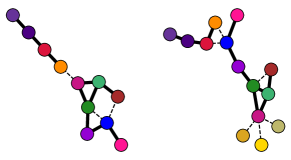
(a) LMCES

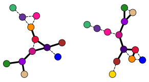
(b) LMCCS

Figure 2: Example graph pairs with node colors indicating the proposed alignments by our models. In Panel (a), we show MCES setup. Here, Nodes are aligned to maximize the number of overlapping edges (indicated as thick black edges). We observe two disconnected components in the MCES setup. In Panel (b), we show MCCS setup. Here, Nodes are aligned to identify largest connected component (identified by thick black edges).

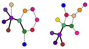
(a) LMCCS

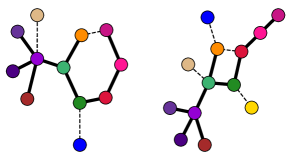
(b) XMCS

Figure 3: Example graph pairs with node colors indicating the proposed alignments by our models LMCCS and XMCS, for the MCCS setup. In Panel (a), LMCCS proposes an alignment which results in an MCCS score of 6. In Panel (b), XMCS proposes an alignment on the same query-corpus pair, which results in an MCCS score of 10. The connected nodes in both cases are identified by thick black edges.

D.5 Training and inference times

Here, we report both the training and inference time (in seconds). The training time is computed for each batch of size 128 (which is the fixed hyperparameter used for the numbers reported in the paper). Inference time is computed for the entire test set of 100 query graphs and 800 corpus graphs, with the maximum possible batch size allowed by our GPU - Nvidia TITAN X (Pascal).

Method	Training Time per batch (in secs)	Inference time on test(in secs)
GEN	0.037	5.937
SimGNN	0.073	24.671
GraphSim	0.125	23.284
NeuroMatch	0.027	6.532
GOTSim	0.259	72.590
IsoNet	0.069	13.956
GMN	0.426	99.542
LMCES	0.109	28.129
LMCCS	0.074	13.776
XMCS	0.159	31.101

Table 14: Training and inference time

We observe that: (1) Among the late interaction models, both LMCCS and LMCES are significantly faster than GOTSim. This is because GOTSim uses a combinatorial solver, which does not allow for batched processing and results in significant slowdown. (2) LMCES is comparable to GraphSim and SimGNN, in both training and inference times, while affording significantly better performance. (3) LMCCS is comparable to IsoNet in training and inference times, and is significantly faster than SimGNN, GraphSim and GOTSim. (4) GEN and NeuroMatch are significantly faster than all late interaction models in terms of training and inference times. However, as shown in Table 1 of the main paper, both these models are outperformed by LMCCS,LMCES and IsoNet in most of the datasets. (5) Among the early interaction models, XMCS is 3X faster than GMN. The reason for this is explained in lines 338-344 in our main paper.

It is true that we performed experiments on graphs of size < 20, driven by the needs of practical graph retrieval applications like molecular fingerprint detection, object detection in images, etc. However, our method can easily scale beyond $|V|=20$, as follows:

Inference Time (in sec)	Current Size	$|V|=30$	$|V|=50$	$|V|=70$	$|V|=100$
LMCES	0.036	0.048	0.052	0.071	0.106
LMCCS	0.022	0.031	0.039	0.042	0.064
XMCS	0.067	0.071	0.085	0.095	0.131

Table 15: Scalability for large graphs

References

- Goyal et al. [2020] Kunal Goyal, Utkarsh Gupta, Abir De, and Soumen Chakrabarti. Deep neural matching models for graph retrieval. In Proceedings of the 43rd International ACM SIGIR Conference on Research and Development in Information Retrieval, pages 1701–1704, 2020.
- Cereto-Massagué et al. [2015] Adrià Cereto-Massagué, María José Ojeda, Cristina Valls, Miquel Mulero, Santiago Garcia-Vallvé, and Gerard Pujadas. Molecular fingerprint similarity search in virtual screening. Methods, 71:58–63, 2015.
- Ohlrich et al. [1993] Miles Ohlrich, Carl Ebeling, Eka Ginting, and Lisa Sather. Subgemini: Identifying subcircuits using a fast subgraph isomorphism algorithm. In Proceedings of the 30th International Design Automation Conference, pages 31–37, 1993.
- Wong [1992] Edward K Wong. Model matching in robot vision by subgraph isomorphism. Pattern Recognition, 25(3):287–303, 1992.
- Johnson et al. [2015] Justin Johnson, Ranjay Krishna, Michael Stark, Li-Jia Li, David Shamma, Michael Bernstein, and Li Fei-Fei. Image retrieval using scene graphs. In Proceedings of the IEEE conference on computer vision and pattern recognition, pages 3668–3678, 2015.
- Li et al. [2019] Yujia Li, Chenjie Gu, Thomas Dullien, Oriol Vinyals, and Pushmeet Kohli. Graph matching networks for learning the similarity of graph structured objects. In International conference on machine learning, pages 3835–3845. PMLR, 2019.
- Bai et al. [2019] Yunsheng Bai, Hao Ding, Song Bian, Ting Chen, Yizhou Sun, and Wei Wang. Simgnn: A neural network approach to fast graph similarity computation. In Proceedings of the Twelfth ACM International Conference on Web Search and Data Mining, pages 384–392, 2019.
- Bai et al. [2020] Yunsheng Bai, Hao Ding, Ken Gu, Yizhou Sun, and Wei Wang. Learning-based efficient graph similarity computation via multi-scale convolutional set matching. In Proceedings of the AAAI Conference on Artificial Intelligence, volume 34, pages 3219–3226, 2020.
- Doan et al. [2021] Khoa D Doan, Saurav Manchanda, Suchismit Mahapatra, and Chandan K Reddy. Interpretable graph similarity computation via differentiable optimal alignment of node embeddings. pages 665–674, 2021.
- Peng et al. [2021] Yun Peng, Byron Choi, and Jianliang Xu. Graph edit distance learning via modeling optimum matchings with constraints. 2021.
- Lou et al. [2020a] Zhaoyu Lou, Jiaxuan You, Chengtao Wen, Arquimedes Canedo, Jure Leskovec, et al. Neural subgraph matching. arXiv preprint arXiv:2007.03092, 2020a.
- Roy et al. [2022] Indradyumna Roy, Venkata Sai Velugoti, Soumen Chakrabarti, and Abir De. Interpretable neural subgraph matching for graph retrieval. AAAI, 2022.
- Zeng et al. [2009] Zhiping Zeng, Anthony KH Tung, Jianyong Wang, Jianhua Feng, and Lizhu Zhou. Comparing stars: On approximating graph edit distance. Proceedings of the VLDB Endowment, 2(1):25–36, 2009.
- Myers et al. [2000] Richard Myers, RC Wison, and Edwin R Hancock. Bayesian graph edit distance. IEEE Transactions on Pattern Analysis and Machine Intelligence, 22(6):628–635, 2000.
- Gao et al. [2010] Xinbo Gao, Bing Xiao, Dacheng Tao, and Xuelong Li. A survey of graph edit distance. Pattern Analysis and applications, 13(1):113–129, 2010.
- Bahiense et al. [2012] Laura Bahiense, Gordana Manić, Breno Piva, and Cid C De Souza. The maximum common edge subgraph problem: A polyhedral investigation. Discrete Applied Mathematics, 160(18):2523–2541, 2012.
- Bokhari [1981] Shahid H. Bokhari. On the mapping problem. IEEE Trans. Computers, 30(3):207–214, 1981.
- Raymond et al. [2002a] John W Raymond, Eleanor J Gardiner, and Peter Willett. Rascal: Calculation of graph similarity using maximum common edge subgraphs. The Computer Journal, 45(6):631–644, 2002a.
- Raymond et al. [2002b] John W Raymond, Eleanor J Gardiner, and Peter Willett. Heuristics for similarity searching of chemical graphs using a maximum common edge subgraph algorithm. Journal of chemical information and computer sciences, 42(2):305–316, 2002b.
- Raymond and Willett [2002] John W Raymond and Peter Willett. Maximum common subgraph isomorphism algorithms for the matching of chemical structures. Journal of computer-aided molecular design, 16(7):521–533, 2002.
- Ehrlich and Rarey [2011] Hans-Christian Ehrlich and Matthias Rarey. Maximum common subgraph isomorphism algorithms and their applications in molecular science: a review. Wiley Interdisciplinary Reviews: Computational Molecular Science, 1(1):68–79, 2011.
- Vismara and Valery [2008] Philippe Vismara and Benoît Valery. Finding maximum common connected subgraphs using clique detection or constraint satisfaction algorithms. In International Conference on Modelling, Computation and Optimization in Information Systems and Management Sciences, pages 358–368. Springer, 2008.
- Bryson et al. [2020] Spencer Bryson, Heidar Davoudi, Lukasz Golab, Mehdi Kargar, Yuliya Lytvyn, Piotr Mierzejewski, Jaroslaw Szlichta, and Morteza Zihayat. Robust keyword search in large attributed graphs. Information Retrieval Journal, pages 1–23, 2020. URL https://doi.org/10.1007/s10791-020-09379-9.
- Zhu et al. [2022] Yuanyuan Zhu, Qian Zhang, Lu Qin, Lijun Chang, and Jeffrey Xu Yu. Cohesive subgraph search using keywords in large networks. IEEE Transactions on Knowledge and Data Engineering, 34:178–191, 2022. URL http://ieeexplore.ieee.org/stamp/stamp.jsp?tp=&arnumber=9028268.
- Englert and Kovács [2015] Péter Englert and Péter Kovács. Efficient heuristics for maximum common substructure search. Journal of chemical information and modeling, 55(5):941–955, 2015.
- Blindell et al. [2015] Gabriel Hjort Blindell, Roberto Castañeda Lozano, Mats Carlsson, and Christian Schulte. Modeling universal instruction selection. In Principles and Practice of Constraint Programming - 21st International Conference, CP 2015, pages 609–626, 2015.
- Sevegnani and Calder [2015] Michele Sevegnani and Muffy Calder. Bigraphs with sharing. Theoretical Computer Science, 577:43–73, 2015.
- Jiang and Ngo [2003] Hui Jiang and Chong-Wah Ngo. Image mining using inexact maximal common subgraph of multiple args. In International conference on visual information system, volume 2, page 3, 2003.
- Hati et al. [2016] Avik Hati, Subhasis Chaudhuri, and Rajbabu Velmurugan. Image co-segmentation using maximum common subgraph matching and region co-growing. In Computer Vision - ECCV 2016 - 14th European Conference, pages 736–752, 2016.
- Shearer et al. [2001] Kim Shearer, Horst Bunke, and Svetha Venkatesh. Video indexing and similarity retrieval by largest common subgraph detection using decision trees. Pattern Recognition, 34(5):1075–1091, 2001.
- Ercal et al. [1990] Fikret Ercal, J Ramanujam, and P Sadayappan. Task allocation onto a hypercube by recursive mincut bipartitioning. Journal of Parallel and Distributed Computing, 10(1):35–44, 1990.
- Marenco [2002] Javier Marenco. A generalization of independent set inequalities for the mapping polytope. Proceedings of CLAIO, 2002.
- Marenco [2006] Javier Marenco. New facets of the mapping polytope. Proceedings of CLAIO, 2006.
- McCreesh et al. [2017] Ciaran McCreesh, Patrick Prosser, and James Trimble. A partitioning algorithm for maximum common subgraph problems. In The Twenty-Sixth International Joint Conference on Artificial Intelligence, IJCAI 2017, pages 712–719, 2017.
- McCreesh et al. [2016] Ciaran McCreesh, Samba Ndojh Ndiaye, Patrick Prosser, and Christine Solnon. Clique and constraint models for maximum common (connected) subgraph problems. In International Conference on Principles and Practice of Constraint Programming, pages 350–368. Springer, 2016.
- Hoffmann et al. [2017] Ruth Hoffmann, Ciaran McCreesh, and Craig Reilly. Between subgraph isomorphism and maximum common subgraph. In Proceedings of the AAAI Conference on Artificial Intelligence, volume 31, 2017.
- Bonnici et al. [2013] Vincenzo Bonnici, Rosalba Giugno, Alfredo Pulvirenti, Dennis Shasha, and Alfredo Ferro. A subgraph isomorphism algorithm and its application to biochemical data. BMC bioinformatics, 14(7):1–13, 2013.
- Duesbury et al. [2017] Edmund Duesbury, John D Holliday, and Peter Willett. Maximum common subgraph isomorphism algorithms. MATCH Communications in Mathematical and in Computer Chemistry, 77(2):213–232, 2017.
- Bai et al. [2021] Yunsheng Bai, Derek Xu, Yizhou Sun, and Wei Wang. Glsearch: Maximum common subgraph detection via learning to search. In The 38th International Conference on Machine Learning, ICML 2021, pages 588–598, 2021.
- Nowak et al. [2018] Alex Nowak, Soledad Villar, Afonso S Bandeira, and Joan Bruna. Revised note on learning quadratic assignment with graph neural networks. In 2018 IEEE Data Science Workshop (DSW), pages 1–5. IEEE, 2018.
- Zanfir and Sminchisescu [2018] Andrei Zanfir and Cristian Sminchisescu. Deep learning of graph matching. In Proceedings of the IEEE conference on computer vision and pattern recognition, pages 2684–2693, 2018.
- Wang et al. [2019] Runzhong Wang, Junchi Yan, and Xiaokang Yang. Learning combinatorial embedding networks for deep graph matching. In Proceedings of the IEEE/CVF International Conference on Computer Vision, pages 3056–3065, 2019.
- Tan et al. [2021] Hao-Ru Tan, Chuang Wang, Si-Tong Wu, Tie-Qiang Wang, Xu-Yao Zhang, and Cheng-Lin Liu. Proxy graph matching with proximal matching networks. In Proceedings of the AAAI Conference on Artificial Intelligence, volume 35, pages 9808–9815, 2021.
- Zhao et al. [2021] Kaixuan Zhao, Shikui Tu, and Lei Xu. Ia-gm: A deep bidirectional learning method for graph matching. In Proceedings of the AAAI Conference on Artificial Intelligence, volume 35, pages 3474–3482, 2021.
- Fey et al. [2020] Matthias Fey, Jan E Lenssen, Christopher Morris, Jonathan Masci, and Nils M Kriege. Deep graph matching consensus. arXiv preprint arXiv:2001.09621, 2020.
- Yu et al. [2019] Tianshu Yu, Runzhong Wang, Junchi Yan, and Baoxin Li. Learning deep graph matching with channel-independent embedding and hungarian attention. In International conference on learning representations, 2019.
- Yu et al. [2021] Tianshu Yu, Runzhong Wang, Junchi Yan, and Baoxin Li. Deep latent graph matching. In International Conference on Machine Learning, pages 12187–12197. PMLR, 2021.
- Liu et al. [2021] Linfeng Liu, Michael C Hughes, Soha Hassoun, and Li-Ping Liu. Stochastic iterative graph matching. arXiv preprint arXiv:2106.02206, 2021.
- Qu et al. [2021] Jingwei Qu, Haibin Ling, Chenrui Zhang, Xiaoqing Lyu, and Zhi Tang. Adaptive edge attention for graph matching with outliers. 2021.
- Gilmer et al. [2017] Justin Gilmer, Samuel S Schoenholz, Patrick F Riley, Oriol Vinyals, and George E Dahl. Neural message passing for quantum chemistry. In International conference on machine learning, pages 1263–1272. PMLR, 2017.
- Hamilton et al. [2017] William L Hamilton, Rex Ying, and Jure Leskovec. Inductive representation learning on large graphs. In Proceedings of the 31st International Conference on Neural Information Processing Systems, pages 1025–1035, 2017.
- Kipf and Welling [2016] Thomas N Kipf and Max Welling. Semi-supervised classification with graph convolutional networks. arXiv preprint arXiv:1609.02907, 2016.
- Veličković et al. [2017] Petar Veličković, Guillem Cucurull, Arantxa Casanova, Adriana Romero, Pietro Lio, and Yoshua Bengio. Graph attention networks. arXiv preprint arXiv:1710.10903, 2017.
- Perozzi et al. [2014] Bryan Perozzi, Rami Al-Rfou, and Steven Skiena. Deepwalk: Online learning of social representations. In KDD, pages 701–710, 2014.
- Grover and Leskovec [2016] Aditya Grover and Jure Leskovec. node2vec: Scalable feature learning for networks. In SIGKDD, 2016.
- Verma et al. [2022] Tathagat Verma, Abir De, Yateesh Agrawal, Vishwa Vinay, and Soumen Chakrabarti. Varscene: A deep generative model for realistic scene graph synthesis. In International Conference on Machine Learning, pages 22168–22183. PMLR, 2022.
- Samanta et al. [2020] Bidisha Samanta, Abir De, Gourhari Jana, Vicenç Gómez, Pratim Kumar Chattaraj, Niloy Ganguly, and Manuel Gomez-Rodriguez. Nevae: A deep generative model for molecular graphs. Journal of machine learning research. 2020 Apr; 21 (114): 1-33, 2020.
- Chen et al. [2022] Dexiong Chen, Leslie O’Bray, and Karsten Borgwardt. Structure-aware transformer for graph representation learning. ICML, 2022.
- Cuturi [2013] Marco Cuturi. Sinkhorn distances: Lightspeed computation of optimal transport. Advances in neural information processing systems, 26:2292–2300, 2013.
- Sinkhorn and Knopp [1967] Richard Sinkhorn and Paul Knopp. Concerning nonnegative matrices and doubly stochastic matrices. Pacific Journal of Mathematics, 21(2):343–348, 1967.
- Vlastelica et al. [2019] Marin Vlastelica, Anselm Paulus, Vít Musil, Georg Martius, and Michal Rolínek. Differentiation of blackbox combinatorial solvers. arXiv preprint arXiv:1912.02175, 2019.
- Rolínek et al. [2020] Michal Rolínek, Paul Swoboda, Dominik Zietlow, Anselm Paulus, Vít Musil, and Georg Martius. Deep graph matching via blackbox differentiation of combinatorial solvers. In European Conference on Computer Vision, pages 407–424. Springer, 2020.
- Berthet et al. [2020] Quentin Berthet, Mathieu Blondel, Olivier Teboul, Marco Cuturi, Jean-Philippe Vert, and Francis Bach. Learning with differentiable pertubed optimizers. Advances in neural information processing systems, 33:9508–9519, 2020.
- Karalias and Loukas [2020] Nikolaos Karalias and Andreas Loukas. Erdos goes neural: an unsupervised learning framework for combinatorial optimization on graphs. Advances in Neural Information Processing Systems, 33:6659–6672, 2020.
- Kotary et al. [2021] James Kotary, Ferdinando Fioretto, Pascal Van Hentenryck, and Bryan Wilder. End-to-end constrained optimization learning: A survey. arXiv preprint arXiv:2103.16378, 2021.
- Pramanik et al. [2021] Soumajit Pramanik, Jesujoba Oluwadara Alabi, Rishiraj Saha Roy, and Gerhard Weikum. Uniqorn: Unified question answering over rdf knowledge graphs and natural language text. ArXiv, abs/2108.08614, 2021. URL https://arxiv.org/pdf/2108.08614.pdf.
- Cormen et al. [2009] Thomas H. Cormen, Charles E. Leiserson, Ronald L. Rivest, and Clifford Stein. Introduction to Algorithms, 3rd Edition. 2009.
- Mena et al. [2018] Gonzalo Mena, David Belanger, Scott Linderman, and Jasper Snoek. Learning latent permutations with gumbel-sinkhorn networks. arXiv preprint arXiv:1802.08665, 2018. URL https://arxiv.org/pdf/1802.08665.pdf.
- Liu et al. [2020] Yanli Liu, Chu-Min Li, Hua Jiang, and Kun He. A learning based branch and bound for maximum common subgraph related problems. In Proceedings of the AAAI Conference on Artificial Intelligence, volume 34, pages 2392–2399, 2020.
- Hariharan et al. [2011] Ramesh Hariharan, Anand Janakiraman, Ramaswamy Nilakantan, Bhupender Singh, Sajith Varghese, Gregory Landrum, and Ansgar Schuffenhauer. Multimcs: a fast algorithm for the maximum common substructure problem on multiple molecules. Journal of chemical information and modeling, 51(4):788–806, 2011.
- Li et al. [2015] Yujia Li, Daniel Tarlow, Marc Brockschmidt, and Richard Zemel. Gated graph sequence neural networks. arXiv preprint arXiv:1511.05493, 2015.
- Morris et al. [2020] Christopher Morris, Nils M. Kriege, Franka Bause, Kristian Kersting, Petra Mutzel, and Marion Neumann. Tudataset: A collection of benchmark datasets for learning with graphs. In ICML 2020 Workshop on Graph Representation Learning and Beyond (GRL+ 2020), 2020. URL www.graphlearning.io.
- Lou et al. [2020b] Zhaoyu Lou, Jiaxuan You, Chengtao Wen, Arquimedes Canedo, Jure Leskovec, et al. Neural subgraph matching. arXiv preprint arXiv:2007.03092, 2020b.
- Hagberg et al. [2008] Aric Hagberg, Pieter Swart, and Daniel S Chult. Exploring network structure, dynamics, and function using networkx. Technical report, Los Alamos National Lab.(LANL), Los Alamos, NM (United States), 2008.
- Kendall [1938] Maurice G Kendall. A new measure of rank correlation. Biometrika, 30(1/2):81–93, 1938.