Synthetic Blip Effects:
Generalizing Synthetic Controls for the
Dynamic Treatment Regime

Abstract

We propose a generalization of the synthetic control and synthetic interventions methodology to the dynamic treatment regime. We consider the estimation of unit-specific treatment effects from panel data collected via a dynamic treatment regime and in the presence of unobserved confounding. That is, each unit receives multiple treatments sequentially, based on an adaptive policy, which depends on a latent endogenously time-varying confounding state of the treated unit. Under a low-rank latent factor model assumption and a technical overlap assumption we propose an identification strategy for any unit-specific mean outcome under any sequence of interventions. The latent factor model we propose admits linear time-varying and time-invariant dynamical systems as special cases. Our approach can be seen as an identification strategy for structural nested mean models under a low-rank latent factor assumption on the blip effects. Our method, which we term “synthetic blip effects”, is a backwards induction process, where the blip effect of a treatment at each period and for a target unit is recursively expressed as linear combinations of blip effects of a carefully chosen group of other units that received the designated treatment. Our work avoids the combinatorial explosion in the number of units that would be required by a vanilla application of prior synthetic control and synthetic intervention methods in such dynamic treatment regime settings.

1 Introduction

In many observational studies, units undergo multiple treatments over a period of time; patients are treated with multiple therapies, customers are exposed to multiple advertising campaigns, governments implement multiple policies, sequentially. Many times these interventions happen in a data adaptive manner, where treatment assignment depends on the current state of the treated unit and on past treatments. A common policy question that arises is what would have been the expected outcome under an alternative policy or course of action. Performing counterfactual analysis from such observational data with multiple sequentially and adaptively assigned treatments is the topic of a long literature on causal inference, known as the dynamic treatment regime.

Dynamic treatment effects with unobserved confounding. Typical approaches for identification in the dynamic treatment regime require a strong sequential exogeneity assumption, where the treatment decision at each period, essentially only depends on an observable state. This assumption is a generalization of the standard conditional exogeneity assumption in the static treatment regime. However, most observational datasets are plagued with unobserved confounding. Many techniques exist for dealing with unobserved confounding in static treatment regimes (such as instrumental variables, differences-in-differences, regression discontinuity designs, synthetic controls). However, approaches to dealing with unobserved confounding in the dynamic treatment regime is a much less explored area. Recent work, for instance, explores an extension of the differences-in-differences approach to the dynamic treatment regime Shahn et al., (2022).

Synthetic controls/interventions in the dynamic treatment regime. In this work, we present the first extension of the synthetic controls literature to the dynamic treatment regime. Synthetic controls method Abadie and Gardeazabal, (2003); Abadie et al., (2010) —and its generalization to synthetic interventions Agarwal et al., 2020b —is a commonly used empirical approach to dealing with unobserved confounding from observational panel data. However, the existing literature assumes that units are treated only once or in a non-adaptive manner. This limits the applicability of the technique to policy relevant settings where multiple interventions occur sequentially over a period of time. Our work proposes an extension of the synthetic controls and synthetic interventions method, that allows the identification of mean counterfactual outcomes under any treatment sequence, even when the observational data came from an adaptive dynamic treatment policy. Similar to the synthetic interventions framework, our work assumes that the panel data stem from a low-rank data generation model and that the latent factors capture the unobserved confounding signals. In the static regime, the low rank assumption together with a technical overlap assumption allows one to express each unit’s mean outcomes under any sequence of interventions as linear combinations of the observed outcomes of a carefully chosen sub-group of other units. We extend this idea to the dynamic treatment regime under a low-rank linear structural nested mean model assumption. Our work can also be viewed as extending the g-estimation framework for structural nested mean models Robins, (2004); Vansteelandt and Joffe, (2014); Lewis and Syrgkanis, (2020) to handle unobserved confounding under a low-rank structure. Thus our work helps connect the literature on synthetic controls with that of structural nested mean models.

Overview of methodology. The key idea of our identification strategy is to express the mean outcome for a unit under a sequence of interventions as an additive function of “blip” effects for that sequence. The blip effect of an intervention at a given period can be thought of as the treatment effect of that intervention compared to a baseline intervention for that specific period, assuming a common sequence of interventions for all other time periods. Subsequently, our low-rank assumption and a recursive argument allows us to identify the blip effect of each treatment for each unit and time period. Our procedure can be viewed as a dynamic programming method where a synthetic control type procedure is used to compute “synthetic blip effects” at each step of the dynamic program to identify time period specific causal quantities, which are subsequently used to build the overall counterfactual quantity of estimating the outcome of any unit under any sequence of interventions.

1.1 Related Work

Panel data methods in econometrics. This is a setting where one gets repeated measurements of multiple heterogeneous units over say $T$ time steps. Prominent frameworks include differences-in-differences Ashenfelter and Card, (1984); Bertrand et al., (2004); Angrist and Pischke, (2009) and synthetic controls Abadie and Gardeazabal, (2003); Abadie et al., (2010); Hsiao et al., (2012); Doudchenko and Imbens, (2016); Athey et al., (2021); Li and Bell, (2017); Xu, (2017); Amjad et al., (2018, 2019); Li, (2018); Arkhangelsky et al., (2020); Bai and Ng, (2020); Ben-Michael et al., (2020); Chan and Kwok, (2020); Chernozhukov et al., (2020); Fernández-Val et al., (2020); Agarwal et al., 2021b ; Agarwal et al., 2020a . These frameworks estimate what would have happened to a unit that undergoes an intervention (i.e., a “treated” unit) if it had remained under control (i.e., no intervention), in the potential presence of unobserved confounding. That is, they estimate the counterfactual if a treated unit remains under control for all $T$ time steps. This is a restricted case of what we consider in this paper, which is to estimate what happens to a unit under any sequence of interventions over the $T$ time steps. A critical aspect that enables the methods above is the structure between units and time under control. One elegant encoding of this structure is through a latent factor model (also known as an interactive fixed effect model), Chamberlain, (1984); Liang and Zeger, (1986); Arellano and Honore, (2000); Bai, (2003, 2009); Pesaran, (2006); Moon and Weidner, (2015, 2017). In such models, it is posited that there exist low-dimensional latent unit and time factors that capture unit and time specific heterogeneity, respectively, in the potential outcomes. Since the goal in these works is to estimate outcomes under control, no structure is imposed on the potential outcomes under intervention.

In Agarwal et al., 2020b ; Agarwal et al., 2021a , the authors extend this latent factor model to incorporate latent factorization across interventions as well, which allows for identification and estimation of counterfactual mean outcomes under intervention rather than just under control. In Section 3, we do a detailed comparison with the synthetic interventions framework introduced in Agarwal et al., 2020b . This framework was designed for the static regime and has two key limitations for the dynamic treatment regime: (i) The framework does not allow for adaptivity in how treatments are chosen over time. (ii) If there are $A$ possible interventions that can be chosen for each of the $T$ time steps, the synthetic interventions estimator has sample complexity scaling as $A^{T}$ to estimate all possible interventional sequences. The non-adaptivity requirement and the exponential dependence on $T$ makes this estimator not well-suited for dynamic treatments, especially as $T$ grows. We show that by imposing that an intervention at a given time step has an additive effect on future outcomes, i.e., an additive latent factor model, it leads to significant gain in what can be identified and estimated. We study two variants, a time-varying and time-invariant version, which nest the classical linear time-varying and linear time-invariant dynamical system models as special cases, respectively. We establish an identification result and a propose an associated estimator to infer all $A^{T}$ counterfactual trajectories per unit. Importantly, our identification result allow the interventions to be selected in an adaptive manner, and the sample complexity of the estimator no longer has an exponential dependence on $T$.

Another extension of such factor models are “dynamic factor models”, originally proposed in Geweke, (1976). We refer the reader to Stock and Watson, (2011); Chamberlain, (2022) for extensive surveys, and see Imbens et al., (2021) for a recent analysis of such time-varying factor models in the context of synthetic controls. These models are similar in spirit to our setting in that they allow outcomes for a given time period to be dependent on the outcome for lagged time periods in an autoregressive manner. To model this phenomenon, dynamic factor models explicitly express the time-varying factor as an autoregressive process. However, the target causal parameter in these works is significantly different—they focus on identifying the latent factors and/or forecasting. There is less emphasis on estimating counterfactual mean outcomes for a given unit under different sequences of interventions.

Linear dynamical systems. Linear dynamical systems are an extensively studied class of models in control and systems theory, and are used as linear approximations to many non–linear systems that nevertheless work well in practice. A seminar work in the study of linear dynamical systems is Kalman, (1960), which introduced the Kalman filter as a robust solution to identifying and estimating the linear parameters that defined the system. We refer the reader to the classic and more recent survey of the analysis of such systems in Ljung, (1999) and Hardt et al., (2016), respectively. Previous works generally assume that (i) the system is driven through independent, and identically distributed (i.i.d) mean-zero sub-Gaussian noise at each time step, and (ii) access to both the outcome variable and a meaningful per-time step state, which are both used in estimation. In comparison, we allow for confounding, i.e., the per time step actions chosen can be correlated with the state of the system in an unknown manner, and we do not assume access to a per-time step state, just the outcome variable. To tackle this setting, we show that linear dynamical systems, both time-varying and time-invariant versions, are special cases of the latent factor model that we propose. The recursive “synthetic blip effects” identification strategy allows to estimate mean counterfactual outcomes under any sequence of interventions without first having to do system identification, and despite unobserved confounding.

1.2 Setting & Notation

Notation. $[R]$ denotes $\{1,\dots,R\}$ for $R\in\mathbb{N}$. $[R_{1},R_{2}]$ denotes $\{R_{1},\dots,R_{2}\}$ for $R_{1},R_{2}\in\mathbb{N}$, with $R_{1}<R_{2}$. $[R]_{0}$ denotes$\{0,\dots,R\}$ for $R\in\mathbb{N}$. For vectors $a,b\in\mathbb{R}^{d}$, $\left\langle a,b\right\rangle$ denotes the inner product of $a$ and $b$. For a vector $a$, we define $a^{\prime}$ as its transpose.

Setup. Let there be $N$ heterogeneous units. We collect data over $T$ time steps for each unit.

Observed outcomes. For each unit and time period $n,t$, we observe $Y_{n,t}\in\mathbb{R}$, which is the outcome of interest.

Actions. For each $n\in[N]$ and $t\in[T]$, we observe actions $A_{n,t}\in[\mathcal{A}]$, where $\mathcal{A}\in\mathbb{N}$. Importantly, we allow $A_{n,t}$ to be categorical, i.e., it can simply serve as a unique identifier for the action chosen. We note that traditionally in dynamical systems, it is assumed we know the exact action vector in $\mathbb{R}^{p}$, where $p$ is the dimension of the action space, rather than just a unique identifier for it. For a sequence of actions $(a_{1},\dots,a_{t})$, denote it by $\bar{a}^{t}\in[\mathcal{A}]^{t}$; denote $(a_{t},\dots,a_{T})$ by $\underline{a}^{t}\in[\mathcal{A}]^{T-t}$. Define $\bar{A}_{n}^{t},\underline{A}_{n}^{t}$ analogously to $\bar{a}^{t},\underline{a}^{t}$, respectively, but now with respect to the observed sequence of actions $A_{n,t}$.

Control & interventional period. For each unit $n$, we assume there exists $t^{*}_{n}\in[1,T]$ before which it is in “control”. We denote the control action at time step $t$ as $0_{t}\in[\mathcal{A}]$. Note $0_{\ell}$ and $0_{t}$ for $\ell\neq t$, do not necessarily have to equal each other. For $t\in[T]$, denote $\bar{0}^{t}=(0_{1},\dots,0_{t})$ and $\underline{0}^{t}=(0_{t},\dots,0_{T})$. For $t<t^{*}_{n}$, we assume $A_{n,t}=0_{t}$, i.e., $\bar{A}_{n}^{t^{*}_{n}-1}=\bar{0}^{t^{*}_{n}-1}$. That is, during the control period all units are under a common sequence of actions, but for $t\geq t^{*}_{n}$, each unit $n$ can undergo a possibly different sequence of actions from all other units, denoted by $\underline{A}^{t^{*}_{n}}_{n}$. Note that if $t^{*}_{n}=1$, then unit $n$ is never in the control period.

Counterfactual outcomes. As stated earlier, for each unit and time period $n,t$, we observe $Y_{n,t}\in\mathbb{R}$, which is the outcome of interest. We denote the potential outcome if unit $n$ had instead undergone $\bar{a}^{t}$ as $Y_{n,t}^{(\bar{a}^{t})}$. More generally, we denote the potential outcome $Y_{n,t}^{(\bar{A}^{\ell}_{n},\underline{a}^{\ell+1})}$ if unit $n$ receives the observed sequence of actions $\bar{A}^{\ell}_{n}$ till time step $\ell$, and then instead undergoes $\underline{a}^{\ell+1}$ for the remaining $t-\ell$ time steps.

We make the standard “stable unit treatment value assumption” (SUTVA) as follows.

Assumption 1 (Sequential Action SUTVA).

For all $n\in[N],t\in[T],\ell\in[t],\bar{a}^{t}\in[\mathcal{A}]^{t}$:

$$Y^{(\bar{A}^{\ell}_{n},\underline{a}^{\ell+1})}_{n,t}=\sum_{\bar{\alpha}^{\ell}\in[\mathcal{A}]^{\ell}}Y^{(\bar{\alpha}^{\ell},\underline{a}^{\ell+1})}_{n,t}\cdot\mathds{1}(\bar{A}^{\ell}_{n}=\bar{\alpha}^{\ell})$$

Further, for all $\bar{A}^{t}_{n}\in[\mathcal{A}]^{t}$:

$$Y^{(\bar{A}^{t}_{n})}_{n,t}=Y_{n,t}.$$

As an immediate implication, $Y^{(\bar{\alpha}^{\ell},\bar{a}^{\ell+1})}_{n,t}\mid\bar{A}^{\ell}_{n}=\bar{\alpha}^{\ell}$ equals $Y^{(\bar{A}^{\ell}_{n},\underline{a}^{\ell+1})}_{n,t}\mid\bar{A}^{\ell}_{n}=\bar{a}^{\ell}$, and $Y^{(\bar{a}^{t})}_{n,t}\mid\bar{A}^{t}_{n}=\bar{a}^{t}$ equals $Y_{n,t}\mid\bar{A}^{t}_{n}=\bar{a}^{t}$.

Goal. Our goal is to accurately estimate the potential outcome if a given unit $n$ had instead undergone $\bar{a}^{T}$ (instead of the actual observed sequence $\bar{A}_{n}^{T}$), for any given sequence of actions $\bar{a}^{T}$ over $T$ times steps. That is, for all $n\in[N]$ $\bar{a}^{T}\in[\mathcal{A}]^{T}$, our goal is to estimate $Y_{n,T}^{(\bar{a}^{T})}.$ We more formally define the target causal parameter in Section 2.

2 Latent Factor Model in the Dynamic Treatment Regime

We now present a novel latent factor model for causal inference with dynamic treatments. Towards that, we first define the collection of latent factors that are of interest.

Definition 1 (Latent factors).

For a given unit $n$ and time step $t$, denote its latent factor as $v_{n,t}$. For a given sequence of actions over $t$ time steps, $\bar{a}^{t}$, denote its associated latent factor as $w_{\bar{a}^{t}}$. Denote the collection of latent factors as

$$\mathcal{LF}\coloneqq\left\{v_{n,t}\right\}_{n\in[N],t\in[T]}\cup\left\{w_{\bar{a}^{t}}\right\}_{\bar{a}^{t}\in[\mathcal{A}]^{t},\ t\in[T]}.$$

Here $v_{n,t},w_{\bar{a}^{t}}\in\mathbb{R}^{d(t)}$, where $d(t)$ is allowed to depend on $t$.

Assumption 2 (General factor model).

Assume $\forall\ n\in[N]$, $t\in[T],\bar{a}^{t}\in[\mathcal{A}]^{t}$,

$$Y^{(\bar{a}^{t})}_{n,t} =\left\langle v_{n,t},w_{\bar{a}^{t}}\right\rangle+\varepsilon^{(\bar{a}^{t})}_{n,t}.$$ (1)

Further,

$$\mathbb{E}[\varepsilon^{(\bar{a}^{t})}_{n,t}\mid\mathcal{LF}]=0$$ (2)

In (1), the key assumption made is that $v_{n,t}$ does not depend on the action sequence $\bar{a}^{t}$, while $w_{\bar{a}^{t}}$ does not depend on unit $n$. That is, $v_{n,t}$ captures the unit $n$ specific latent heterogeneity in determining the expected conditional potential outcome $\mathbb{E}[Y^{(\bar{a}^{t})}_{n,t}\mid\mathcal{LF}]$; $w_{\bar{a}^{t}}$ follows a similar intuition but with respect to the action sequence $\bar{a}^{t}$. This latent factorization will be key in all our identification and estimation algorithms, and the associated theoretical results. An interpretation of $\varepsilon^{(\bar{a}^{t})}_{n,t}$ is that it represents the component of the potential outcome $Y^{(\bar{a}^{T})}_{n,T}$ that is not factorizable into the latent factors represented by $\mathcal{LF}$; alternatively, it helps model the inherent randomness in the potential outcomes $Y^{(\bar{a}^{T})}_{n,T}$. In Sections 4 and 5 below, we show how various standard models of dynamical systems are a special case of our proposed factor model in Assumption 2.

Target Causal Parameter

Our target causal parameter is to estimate for all units $n\in[N]$ and any action sequence $\bar{a}^{T}\in[\mathcal{A}]^{T}$,

$$\mathbb{E}[Y^{(\bar{a}^{T})}_{n,T}~{}|~{}\mathcal{LF}],$$ (target causal parameter)

i.e., the expected potential outcome conditional on the latent factors, $\mathcal{LF}$. In total this amounts to estimating $N\times|\mathcal{A}|^{T}$ different (expected) potential outcomes, which we note grows exponentially in $T$.

3 Limitations of Synthetic Interventions Approach

Given that our goal is to bring to bear a novel factor model perspective to the dynamic treatment effects literature, we first exposit on some of the limitations of the current methods from the factor model literature that were designed for the static interventions regime, i.e., where an intervention is done only once at a particular time step. We focus on the synthetic interventions (SI) framework Agarwal et al., 2020b , which is a recent generalization of the popular synthetic controls framework from econometrics. In particular, we provide an identification argument which builds upon the SI framework Agarwal et al., 2020b and then discuss its limitations.

3.1 Identification Strategy via SI Framework

3.1.1 Notation and Assumptions

Donor units. To explain the identification strategy, we first need to define a collection of subsets of units based on: (i) the action sequence they receive; (ii) the correlation between their potential outcomes and the chosen actions. These subsets are defined as follows.

Definition 2 (SI donor units).

For $\bar{a}^{T}\in[\mathcal{A}]^{T}$,

$$\mathcal{I}^{\bar{a}^{T}} \coloneqq\{j\in[N]:(i)\ \bar{A}^{T}_{j}=\bar{a}^{T},\ (ii)\ \ \forall\ \bar{\alpha}^{T}\in[\mathcal{A}]^{T},\ \ \mathbb{E}[\varepsilon^{(\bar{\alpha}^{T})}_{j,T}\mid\bar{A}^{T}_{j},\mathcal{LF}]=0\}.$$ (3)

$\mathcal{I}^{\bar{a}^{T}}$ refers to units that receive exactly the sequence $\bar{a}^{T}$. Further, we require that for these particular units, the action sequence was chosen such that $\forall\ \bar{\alpha}^{T}\in[\mathcal{A}]^{T},\ \mathbb{E}[\varepsilon^{(\bar{\alpha}^{T})}_{j,T}\mid\bar{A}^{T}_{j},\mathcal{LF}]=\mathbb{E}[\varepsilon^{(\bar{\alpha}^{T})}_{j,T}\mid\mathcal{LF}]=0$, i.e., $\varepsilon^{(\bar{\alpha}^{T})}_{j,T}$ is conditionally mean independent of the action sequence $\bar{A}^{T}_{j}$ unit $j$ receives. Note a sufficient condition for property (ii) above is that $\forall\ \bar{\alpha}^{T}\in[\mathcal{A}]^{T},\ \ Y^{(\bar{\alpha}^{T})}_{j,T}\perp\bar{A}^{T}_{j}\mid\mathcal{LF}$. That is, for these units, the action sequence for the entire time period $T$ is chosen at $t=0$ conditional on the latent factors, i.e., the policy for these units is not adaptive (cannot depend on observed outcomes $Y_{j,t}$ for $t\in[T]$).

Assumption 3.

$\forall n\in[N],\bar{a}^{T}\in[\mathcal{A}]^{T}$ suppose that $v_{n,T}$ satisfies a well-supported condition, i.e., there exists linear weights $\beta^{n,\mathcal{I}^{\bar{a}^{T}}}\in\mathbb{R}^{|\mathcal{I}^{\bar{a}^{T}}|}$ such that:

$$v_{n,T}=\sum_{j\in\mathcal{I}^{\bar{a}^{T}}}\beta_{j}^{n,\mathcal{I}^{\bar{a}^{T}}}v_{j,T}.$$ (well-supported factors)

Assumption 3 essentially states that for a given sequence of interventions $\bar{a}^{T}\in[\mathcal{A}]^{T}$, the latent factor for the target unit $v_{n,T}$ lies in the linear span of the latent factors $v_{j,T}$ associated with the “donor” units in $\mathcal{I}^{\bar{a}^{T}}$. Note by Theorem 4.6.1 of Vershynin, (2018), if the $\{v_{j,T}\}_{j\in[N]}$ are sampled as independent, mean zero, sub-Gaussian vectors,then $\text{span}(\{v_{j}:j\in\mathcal{I}^{\bar{a}^{T}})\})=\mathbb{R}^{d(T)}$ with high probability as $|\mathcal{I}^{\bar{a}^{T}}|$ grows, and if $|\mathcal{I}^{\bar{a}^{T}}|\gg d(T)$ (recall $d(T)$ is the dimension of $v_{n,T}$).

3.1.2 Identification Result

We then have an identification theorem, which states that the (target causal parameter) can expressed as a function of observed outcomes. It is an adaptation of the identification argument in Agarwal et al., 2020b .

Theorem 1 (SI Identification Strategy).

Let Assumptions 1, 2, and 3 hold. Then, for $\forall n\in[N],\bar{a}^{T}\in[\mathcal{A}]^{T}$, the mean counterfactual outcome can be expressed as:

$$\mathbb{E}[Y_{n,T}^{(\bar{a}^{T})}\mid\mathcal{LF}]=~{} \mathbb{E}\left[\sum_{j\in\mathcal{I}^{\bar{a}^{T}}}\beta_{j}^{n,\mathcal{I}^{\bar{a}^{T}}}Y_{j,T}\mid\mathcal{LF},\mathcal{I}^{\bar{a}^{T}}\right].$$

Interpretation of identification result.

Theorem 1 establishes that to estimate the mean counterfactual outcome of unit $n$ under the action sequence $\bar{a}^{T}$, select all donors that received that sequence, i.e., $\bar{A}^{T}=\bar{a}^{T}$, and for whom we know that their action sequence was not adaptive. The target causal parameter then is simply a linear re-weighting of the observed outcomes $(Y_{j,T})_{j\in\mathcal{I}^{\bar{a}^{T}}}$, where these linear weights $\beta_{j}^{n,\mathcal{I}^{\bar{a}^{T}}}$ express the latent factor $v_{n,T}$ for unit $n$ as a linear combination of $\{v_{j,T}\}_{j\in\in\mathcal{I}^{\bar{a}^{T}}}$.

3.1.3 SI Identification Strategy: Donor Sample Complexity & Exogeneity Conditions

Donor sample complexity. To estimate $\mathbb{E}[Y^{(\bar{a}^{T})}_{n,T}~{}|~{}\mathcal{LF}]$ for all units $n\in[N]$ and any action sequence $\bar{a}^{T}\in[\mathcal{A}]^{T}$, this SI identification strategy requires the existence of a sufficiently large subset of donor units $\mathcal{I}^{\bar{a}^{T}}$ for every $\bar{a}^{T}\in[\mathcal{A}]^{T}$. That is, the number of donor units we require will need to scale at the order of $|\mathcal{A}|^{T}$, which grows exponentially in $T$.

Donor exogeneity conditions. Further, the actions picked for these donor units cannot be adaptive as we require $\forall\ \bar{\alpha}^{T}\in[\mathcal{A}]^{T},\ \ \mathbb{E}[\varepsilon^{(\bar{\alpha}^{T})}_{j,T}\mid\bar{A}^{T}_{j},\mathcal{LF}]=0$ for them. See Figure 1 for a directed acyclic graph (DAG) that is consistent with the exogeneity conditions implied by the definition of $\mathcal{I}^{\bar{a}^{T}}$ in (3).

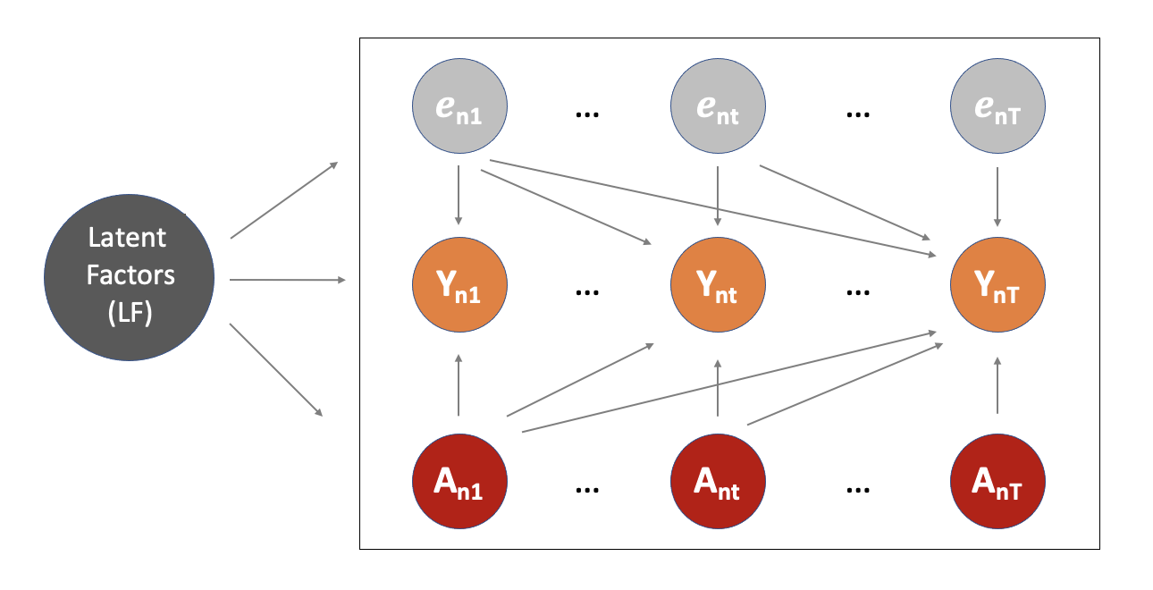
Figure 1: DAG that is consistent with the exogeneity conditions implied by the definition of $\mathcal{I}^{\bar{a}^{T}}$.

Overcoming limitations of SI identification strategy. Given this combinatorial explosion in the number of donor units and the stringent non-adaptivity requirements on these donor units, in the following sections we study how additional structure on the latent factor model gives rise to novel identification strategies, which allows us to reduce the donor sample complexity, and the exogeneity requirements between the chosen actions and the donor units.

4 Linear Time-Varying Latent Factor Model

Motivated by the limitation of the identification strategy in Section 3, we now impose additional structure on the latent factor model as described below. In Section 4.1, we show that a linear time-varying dynamical system is a special case of this factor model. We now state the latent factor model assumption.

Assumption 4 (Linear time-varying (LTV) factor model).

Assume $\forall\ n\in[N]$, $t\in[T],\bar{a}^{t}\in[\mathcal{A}]^{t}$,

$$Y^{(\bar{a}^{t})}_{n,t} =\sum^{t}_{\ell=1}\left\langle\psi^{t,\ell}_{n},w_{a_{\ell}}\right\rangle+\varepsilon^{(\bar{a}^{t})}_{n,t}.$$ (4)

where $\psi^{t,\ell}_{n},w_{a_{\ell}}\in\mathbb{R}^{d}$ for $\ell\in[t]$. Further, let $\mathcal{LF}=\{\psi^{t,\ell}_{n}\}_{n\in[N],t\in[T],\ell\in[t]}\cup\{w_{a}\}_{a\in[\mathcal{A}]}$. Assume,

$$\mathbb{E}[\varepsilon^{(\bar{a}^{t})}_{n,t}\mid\mathcal{LF}]=0$$ (5)

Remark.

Note Assumption 4 implies Assumption 2 holds with

$$v_{n,t}=[\psi^{t,1}_{n},\dots,\psi^{t,t}_{n}],\ w_{\bar{a}^{t}}=[w_{a_{1}},\dots,w_{a_{t}}].$$

Further $d(t)=d\times t$ for $d(t)$ in Definition 1.

We see that there is additional structure in the latent factors. In particular, the effect of action $a_{\ell}$ on $Y^{(\bar{a}^{t})}_{n,t}$ for $\ell\in[t]$ is additive, given by $\langle\psi^{t,\ell}_{n},w_{a_{\ell}}\rangle$. Intuitively, $\psi_{n}^{t,\ell}$ captures the latent unit specific heterogeneity in the potential outcome for unit $n$ at a given time step $t$ for an action taken at time step $\ell\leq t$; analogously $w_{a_{\ell}}$ captures the latent effect of action $a_{\ell}$. This additional structure along will be crucial in the identification strategy we employ in Section 4.2.

4.1 Motivating Example

We show that the classical linear time-varying dynamical system model satisfies Assumption 2. Suppose for all $t\in[T]$, all units $n\in[N]$ obey the following dynamical system for a sequence of actions $\bar{A}^{t}_{n}$ (assume $z_{n,0},w_{A_{n,0}}=0$):

$$A_{n,t} =f_{n}(w_{A_{n,t-1}},\ z^{(\bar{A}_{n}^{t-1})}_{n,t-1}),$$

$$z^{(\bar{A}_{n}^{t})}_{n,t} =\boldsymbol{B}_{n,t}\ z^{(\bar{A}_{n}^{t-1})}_{n,t-1}+\boldsymbol{C}_{n,t}\ w_{A_{n,t}}+\eta_{n,t}$$

$$Y^{(\bar{A}_{n}^{t})}_{n,t} =\left\langle\theta_{n,t},z^{(\bar{A}_{n}^{t})}_{n,t}\right\rangle+\left\langle\tilde{\theta}_{n,t},w_{A_{n,t}}\right\rangle+\tilde{\eta}_{n,t}.$$

Here, $z_{n,t}\in\mathbb{R}^{d}$ is the latent state associated with unit $n$ at time $t$ and $w_{A_{n,t-1}}\in\mathbb{R}^{d}$ is the chosen action at time $t-1$. $\eta_{n,t}\in\mathbb{R}^{d}$ and $\tilde{\eta}_{n,t}\in\mathbb{R}$ represent independent mean-zero random innovations at each time step $t$. $\boldsymbol{B}_{n,t},\boldsymbol{C}_{n,t}\in\mathbb{R}^{d\times d}$ are matrices governing the linear dynamics of $z^{(\bar{A}_{n}^{t})}_{n,t}$. Note $\boldsymbol{B}_{n,t},\boldsymbol{C}_{n,t}$ are specific to time step $t$ and this is what makes this model a time-varying dynamical system. In contrast, in the classic linear time-invariant dynamical system described in Section 5.1 below, $\boldsymbol{B}_{n,t}=\boldsymbol{B}_{n}$ and $\boldsymbol{C}_{n,t}=\boldsymbol{C}_{n}$ for all $t\in[T]$. $\theta_{n,t},\tilde{\theta}_{n,t}\in\mathbb{R}^{d}$ are parameters governing how the outcome of interest $Y^{(\bar{A}_{n}^{t})}_{n,t}$ is a linear function of $z^{(\bar{A}_{n}^{t})}_{n,t}$ and $w_{a_{t}}$, respectively. $f_{n}(\cdot)$ is a function which decides how the next action $w_{A_{n,t}}$ is chosen as a function of the previous action $w_{A_{n,t-1}}$, and current state $z_{n,t}$. We see that due to the input of $z^{(\bar{A}_{n}^{t})}_{n,t}$ in $f_{n}(\cdot)$, i.e., the action sequence is adaptive. As a result, $\eta_{n,\ell}$ is correlated with $A_{n,t}$ for $\ell<t$.

Proposition 1.

Suppose the linear time-varying dynamical system above holds. Assume $z_{n,0},\ w_{a_{0}}=0$. Then we have the following representation,

$$Y^{(\bar{a}^{t})}_{n,t}=\sum^{t}_{\ell=1}\Big{(}\left\langle\psi^{t,\ell}_{n},w_{a_{\ell}}\right\rangle+\varepsilon_{n,t,\ell}\Big{)},$$ (6)

where $\psi^{t,\ell}_{n},w_{a_{\ell}}\in\mathbb{R}^{d}$ for $\ell\in[t]$; here,

$$\psi^{t,\ell}_{n} =\left(\left(\prod^{t}_{k=\ell+1}\boldsymbol{B}_{n,k}\right)\boldsymbol{C}_{n,{\ell}}\right)^{\prime}\theta_{n,t}\quad\text{for}\quad\ell\in[t-1],$$

$$\psi^{t,t}_{n} =\boldsymbol{C}_{n,{t}}^{\prime}\theta_{n,t}+\tilde{\theta}_{n,t},$$

$$\varepsilon_{n,t,\ell} =\left(\left(\prod^{t}_{k=\ell+1}\boldsymbol{B}_{n,k}\right)\eta_{n,\ell}\right)^{\prime}\theta_{n,t}\quad\text{for}\quad\ell\in[t-1],$$

$$\varepsilon_{n,t,t} =\theta_{n,t}^{\prime}\eta_{n,t}+\tilde{\eta}_{n,t}.$$

Therefore, Assumption 4 holds with the additional structure that $\varepsilon^{(\bar{a}^{t})}_{n,t}$ has an additive factorization as $\sum^{t}_{\ell=1}\varepsilon_{n,t,\ell}$, and it is not a function of $a_{\ell}$.

In this example, our target parameter $\mathbb{E}[Y^{(\bar{a}^{T})}_{n,T}~{}|~{}\mathcal{LF}]$ defined in (target causal parameter) translates to the expected potential once we condition on the latent parameters $\psi^{t,\ell}_{n},w_{a_{\ell}}$, which are a function of $\boldsymbol{B}_{n,t},\boldsymbol{C}_{n,t},\theta_{n,t},\tilde{\theta}_{n,t}$. Here the expectation is take with respect to the per-step independent mean-zero random innovations, $\varepsilon_{n,t,\ell}$, which are a function of $[\eta_{n,q},\tilde{\eta}_{n,q}]_{q\geq\ell}$ (and $\boldsymbol{B}_{n,t},\boldsymbol{C}_{n,t},\theta_{n,t},\tilde{\theta}_{n,t}$).

Note that once we re-write this linear time-varying dynamical system in terms of the latent factor representation, we do not need to observe the parameters $z^{(\bar{A}_{n}^{t})}_{n,t}$ and $w_{a_{\ell}}$ to express the potential outcomes in terms of them. The only information we need about $w_{a_{\ell}}$ is a unique identifier, given by $a_{\ell}$. Traditionally, state-based models of linear dynamical systems literature require that both $z^{(\bar{A}_{n}^{t})}_{n,t}$ and $w_{a_{\ell}}$ are perfectly observed. Input-output models for dynamical systems assume that $w_{a_{\ell}}$ is perfectly observed.

4.2 LTV Identification Strategy

In this section we identify $\mathbb{E}[Y_{n,T}^{(\bar{a}^{T})}\mid\mathcal{LF}]$, i.e., represent this expected potential outcome for a target unit $n$ and action sequence $\bar{a}^{T}$ as some function of observed outcomes.

4.2.1 Notation and Assumptions

Notation. We define the following useful notation for any unit $n\in[N]$:

$$\gamma_{n,T,t}(a^{t}):=\left\langle\psi^{T,t}_{n},w_{a_{t}}-w_{0_{t}}\right\rangle$$

$\gamma_{n,T,t}(a^{t})$ can be interpreted as a “blip effect”, i.e., the expected difference in potential outcomes if unit $n$ undergoes the sequence $(\bar{a}^{t},\underline{0}^{t+1})$ instead of $(\bar{a}^{t-1},\underline{0}^{t})$. In particular, note that Assumption 4 implies

$$\mathbb{E}\left[Y^{(\bar{a}^{t},\underline{0}^{t+1})}_{n,T}-Y^{(\bar{a}^{t-1},\underline{0}^{t})}_{n,T}\mid\mathcal{LF}\right] =\mathbb{E}\left[\left\langle\psi^{T,t}_{n},w_{a_{t}}-w_{0_{t}}\right\rangle+\varepsilon^{(\bar{a}^{t},\underline{0}^{t+1})}_{n,T}-\varepsilon^{(\bar{a}^{t-1},\underline{0}^{t})}_{n,T}\mid\mathcal{LF}\right]$$

$$=\left\langle\psi^{T,t}_{n},w_{a_{t}}-w_{0_{t}}\right\rangle\mid\mathcal{LF}.$$

Further, let

$$b_{n,T} :=\sum^{T}_{t=1}\left\langle\psi^{T,t}_{n},w_{0_{t}}\right\rangle.$$

This can be interpreted as the expected potential outcome if unit $j$ remains under the control sequence $\bar{0}^{T}$ till time step $T$. Again, Assumption 4 implies

$$\mathbb{E}\left[Y^{(\bar{0}^{T})}_{n,T}\mid\mathcal{LF}\right] =\mathbb{E}\left[\sum^{T}_{t=1}\left\langle\psi^{T,t}_{n},w_{0_{t}}\right\rangle+\varepsilon^{(\bar{0}^{T})}_{n,T}\mid\mathcal{LF}\right]=\sum^{T}_{t=1}\left\langle\psi^{T,t}_{n},w_{0_{t}}\right\rangle\mid\mathcal{LF}$$ (7)

Assumptions. We now state the various assumptions we need for the identification strategy that we propose next.

Donor sets. We define different subsets of units based on the action sequence they receive that is necessary for our result.

$$\mathcal{I}^{a}_{t}\coloneqq\{j\in[N]: \ (i)\ \bar{A}^{t}_{j}=(0_{1},\dots,0_{t-1},a),$$

$$(ii)\ \forall\ \bar{\alpha}^{T}\in[\mathcal{A}]^{T},\ \mathbb{E}[Y^{(\bar{\alpha}^{T})}_{j,T}\mid\mathcal{LF},\bar{A}^{t}_{j}]=\mathbb{E}[Y^{(\bar{\alpha}^{T})}_{j,T}\mid\mathcal{LF}]\},$$ (8)

$\mathcal{I}^{a}_{t}$ refers to units that remain under the control sequence $(0_{1},\dots,0_{t-1})$ till time step $t-1$, and at time step $t$ receive action $a$ (i.e., $t^{*}_{n}\geq t-1$). Further, we require that for these particular units, the action sequence, $\bar{A}^{t}_{j}$, till time step $t$ was chosen such that $\mathbb{E}[Y^{(\bar{\alpha}^{T})}_{j,T}\mid\mathcal{LF},\bar{A}^{t}_{j}]=\mathbb{E}[Y^{(\bar{\alpha}^{T})}_{j,T}\mid\mathcal{LF}]$, i.e., the potential outcomes are conditionally mean independent of the action sequence $\bar{A}^{t}_{j}$ unit $j$ receives till time step $t$. Of course, a sufficient condition for property (ii) above is that $\forall\ \bar{\alpha}^{T}\in[\mathcal{A}]^{T},\ \ Y^{(\bar{\alpha}^{T})}_{j,T}\perp\bar{A}^{t}_{j}\mid\mathcal{LF}$. That is, for these units, the action sequence till time step $t$ is chosen at $t=0$ conditional on the latent factors, i.e., the policy for these units can only be adaptive from time step $t+1$. Note, given Assumption 4, this property (ii) can be equivalently stated as $\mathbb{E}[\varepsilon^{(\bar{\alpha}^{T})}_{j,T}\mid\mathcal{LF},\bar{A}^{t}_{j}]=\mathbb{E}[\varepsilon^{(\bar{\alpha}^{T})}_{j,T}\mid\mathcal{LF}]=0$.

Assumption 5.

For $n\in[N]$, let $v_{n,T}:=[\psi^{T,1}_{n},\dots,\psi^{T,T}_{n}]$. We assume that for all $n\in[N]$, $v_{n,T}$ satisfies a well-supported condition with respect to the various donor sets, i.e., for all $a\in[\mathcal{A}]$ and $t\in[T]$, there exists $\beta^{n,\mathcal{I}_{t}^{a}}\in\mathbb{R}^{|\mathcal{I}_{t}^{a}|}$ such that

$$v_{n,T}=\sum_{k\in\mathcal{I}_{t}^{a}}\beta_{k}^{n,\mathcal{I}_{t}^{a}}v_{k,T}$$ (LTV well-supported factors)

Assumption 5 requires that for units $n\in[N]$, their latent factors $[\psi^{T,1}_{n},\dots,\psi^{T,T}_{n}]$ are expressible as a linear combination of the units in the donor sets $\mathcal{I}_{t}^{a}$. See the discussion under Assumption 3 in Section 3 justifying such an assumption for settings when $\mathcal{I}_{t}^{a}$ is sufficiently large.

Assumption 6.

For all $n\in[N],t\in[T],\bar{a}^{t}\in[\mathcal{A}]^{t}$,

$$\mathbb{E}\left[Y_{n,T}^{(\bar{a}^{t},\underline{0}^{t+1})}-Y_{n,T}^{(\bar{a}^{t-1},\underline{0}^{t})}\mid\bar{A}_{n}^{t}=\bar{a}^{t},\mathcal{LF}\right]=\gamma_{n,T,t}(a_{t})\mid\mathcal{LF}$$

Note that given Assumption 4, this condition can be equivalently written as

$$\mathbb{E}\left[\varepsilon_{n,T}^{(\bar{a}^{t},\underline{0}^{t+1})}-\varepsilon_{n,T}^{(\bar{a}^{t-1},\underline{0}^{t})}\mid\bar{A}_{n}^{t}=\bar{a}^{t},\mathcal{LF}\right]=0$$

Below we give two sufficient conditions under which Assumption 6 holds.

1. Sufficient condition: Non-action dependent noise. Assumption 6 holds if $\varepsilon_{n,T}^{(\bar{a}^{t},\underline{0}^{t+1})}=\varepsilon_{n,T}^{(\bar{a}^{t-1},\underline{0}^{t})}$, which occurs if $\varepsilon_{n,T}^{(\bar{a}^{t},\underline{0}^{t+1})}$ and $\varepsilon_{n,T}^{(\bar{a}^{t-1},\underline{0}^{t})}$ are not a function of $(\bar{a}^{t},\underline{0}^{t+1})$, and $(\bar{a}^{t-1},\underline{0}^{t})$, respectively. The motivating example of a classic linear time-varying dynamical system given in Section 4.1 satisfies this property.

2. Sufficient condition: Additive action-dependent noise. We now relax the sufficient condition above that $\varepsilon_{n,T}^{(\bar{a}^{t},\underline{0}^{t+1})}$ and $\varepsilon_{n,T}^{(\bar{a}^{t-1},\underline{0}^{t})}$ are not a function of the action sequence. Instead, suppose for all $\bar{a}^{T}\in[\mathcal{A}]^{T}$, $\varepsilon_{n,T}^{(\bar{a}^{T})}=\sum^{T}_{t=1}\eta^{(a_{t})}_{n,t}$, where we assume that conditional on $\mathcal{LF}$, $\eta^{(a_{t})}_{n,t}$ are mutually independent for all $t\in[T]$, and $a_{t}\in[\mathcal{A}]$. Then $\varepsilon_{n,T}^{(\bar{a}^{t},\underline{0}^{t+1})}-\varepsilon_{n,T}^{(\bar{a}^{t-1},\underline{0}^{t})}=\eta^{(a_{t})}_{n,t}-\eta^{(0_{t})}_{n,t}$. In this case, a sufficient condition for Assumption 6 is that

$$\eta^{(a_{t})}_{n,t},\eta^{(0_{t})}_{n,t}\ \mathbin{\mathchoice{\hbox to0.0pt{\hbox{\set@color$\displaystyle\perp$}\hss}\kern 3.46875pt\kern 3.46875pt\hbox{\set@color$\displaystyle\perp$}}{\hbox to0.0pt{\hbox{\set@color$\textstyle\perp$}\hss}\kern 3.46875pt\kern 3.46875pt\hbox{\set@color$\textstyle\perp$}}{\hbox to0.0pt{\hbox{\set@color$\scriptstyle\perp$}\hss}\kern 2.36812pt\kern 2.36812pt\hbox{\set@color$\scriptstyle\perp$}}{\hbox to0.0pt{\hbox{\set@color$\scriptscriptstyle\perp$}\hss}\kern 1.63437pt\kern 1.63437pt\hbox{\set@color$\scriptscriptstyle\perp$}}}\ A_{n,t}\mid\mathcal{LF}.$$

That is, conditional on the latent factors, the action $A_{n,t}$ at time step $t$ is independent of the additional noise $\eta^{(a_{t})}_{n,T,t},\eta^{(0_{t})}_{n,T,t}$ generated at time step $t$. Note, however that $\varepsilon_{n,t}^{(\bar{a}^{t})}\ \mathbin{\mathchoice{\hbox to0.0pt{\hbox{\set@color$\displaystyle\perp$}\hss}\kern 3.46875pt\hbox to10.55551pt{\hss$\displaystyle/$\hss}\kern-10.55551pt\kern 3.46875pt\hbox{\set@color$\displaystyle\perp$}}{\hbox to0.0pt{\hbox{\set@color$\textstyle\perp$}\hss}\kern 3.46875pt\hbox to10.55551pt{\hss$\textstyle/$\hss}\kern-10.55551pt\kern 3.46875pt\hbox{\set@color$\textstyle\perp$}}{\hbox to0.0pt{\hbox{\set@color$\scriptstyle\perp$}\hss}\kern 2.36812pt\hbox to8.22217pt{\hss$\scriptstyle/$\hss}\kern-8.22217pt\kern 2.36812pt\hbox{\set@color$\scriptstyle\perp$}}{\hbox to0.0pt{\hbox{\set@color$\scriptscriptstyle\perp$}\hss}\kern 1.63437pt\hbox to6.66661pt{\hss$\scriptscriptstyle/$\hss}\kern-6.66661pt\kern 1.63437pt\hbox{\set@color$\scriptscriptstyle\perp$}}}\ A_{n,t}\mid\mathcal{LF}$. This is because $\varepsilon_{n,t-1}^{(\bar{a}^{t-1})}$ and $\varepsilon_{n,t}^{(\bar{a}^{t})}$ remain auto-correlated, i.e., . $\varepsilon_{n,t}^{(\bar{a}^{t-1})}\ \mathbin{\mathchoice{\hbox to0.0pt{\hbox{\set@color$\displaystyle\perp$}\hss}\kern 3.46875pt\hbox to10.55551pt{\hss$\displaystyle/$\hss}\kern-10.55551pt\kern 3.46875pt\hbox{\set@color$\displaystyle\perp$}}{\hbox to0.0pt{\hbox{\set@color$\textstyle\perp$}\hss}\kern 3.46875pt\hbox to10.55551pt{\hss$\textstyle/$\hss}\kern-10.55551pt\kern 3.46875pt\hbox{\set@color$\textstyle\perp$}}{\hbox to0.0pt{\hbox{\set@color$\scriptstyle\perp$}\hss}\kern 2.36812pt\hbox to8.22217pt{\hss$\scriptstyle/$\hss}\kern-8.22217pt\kern 2.36812pt\hbox{\set@color$\scriptstyle\perp$}}{\hbox to0.0pt{\hbox{\set@color$\scriptscriptstyle\perp$}\hss}\kern 1.63437pt\hbox to6.66661pt{\hss$\scriptscriptstyle/$\hss}\kern-6.66661pt\kern 1.63437pt\hbox{\set@color$\scriptscriptstyle\perp$}}}\varepsilon_{n,t}^{(\bar{a}^{t})}\mid\mathcal{LF}$. Also, $\varepsilon_{n,t}^{(\bar{a}^{t-1})}\ \mathbin{\mathchoice{\hbox to0.0pt{\hbox{\set@color$\displaystyle\perp$}\hss}\kern 3.46875pt\hbox to10.55551pt{\hss$\displaystyle/$\hss}\kern-10.55551pt\kern 3.46875pt\hbox{\set@color$\displaystyle\perp$}}{\hbox to0.0pt{\hbox{\set@color$\textstyle\perp$}\hss}\kern 3.46875pt\hbox to10.55551pt{\hss$\textstyle/$\hss}\kern-10.55551pt\kern 3.46875pt\hbox{\set@color$\textstyle\perp$}}{\hbox to0.0pt{\hbox{\set@color$\scriptstyle\perp$}\hss}\kern 2.36812pt\hbox to8.22217pt{\hss$\scriptstyle/$\hss}\kern-8.22217pt\kern 2.36812pt\hbox{\set@color$\scriptstyle\perp$}}{\hbox to0.0pt{\hbox{\set@color$\scriptscriptstyle\perp$}\hss}\kern 1.63437pt\hbox to6.66661pt{\hss$\scriptscriptstyle/$\hss}\kern-6.66661pt\kern 1.63437pt\hbox{\set@color$\scriptscriptstyle\perp$}}}\ A_{n,t}\mid\mathcal{LF}$, as the action $A_{n,t}$ can be a function of the observed outcomes $Y_{n,t-1}$.

Sequential conditional exogeneity, SNMMs and MSMs.

We now connect our assumptions more closely to the notation and assumptions used in the structural nested mean model (SNMM) and the marginal structural model (MSM) literatures. A typical assumption in these literatures is sequential conditional exogeneity, which states that for some sequence of random state variables $S_{n,t}$, the treatments are sequentially conditionally exogenous, i.e.:

$$\forall\bar{a}\in[A]^{T}:Y_{n,T}^{(\bar{a})}\mathbin{\mathchoice{\hbox to0.0pt{\hbox{\set@color$\displaystyle\perp$}\hss}\kern 3.46875pt\kern 3.46875pt\hbox{\set@color$\displaystyle\perp$}}{\hbox to0.0pt{\hbox{\set@color$\textstyle\perp$}\hss}\kern 3.46875pt\kern 3.46875pt\hbox{\set@color$\textstyle\perp$}}{\hbox to0.0pt{\hbox{\set@color$\scriptstyle\perp$}\hss}\kern 2.36812pt\kern 2.36812pt\hbox{\set@color$\scriptstyle\perp$}}{\hbox to0.0pt{\hbox{\set@color$\scriptscriptstyle\perp$}\hss}\kern 1.63437pt\kern 1.63437pt\hbox{\set@color$\scriptscriptstyle\perp$}}}\ A_{n,t}\mid\bar{S}^{t-1}_{n},\bar{A}^{t}_{n}=\bar{a}_{t},\mathcal{LF},$$ (9)

where $\bar{S}^{t-1}_{n}=(S_{n,0},\ldots,S_{n,t-1})$. Moreover, assume that the blip effects admit the following factor model representation:

$$\mathbb{E}\left[Y_{n,T}^{(\bar{a}^{t},\underline{0}^{t+1})}-Y_{n,T}^{(\bar{a}^{t-1},\underline{0}^{t})}\mid\bar{S}^{t-1}_{n},\bar{A}_{n}^{t}=\bar{a}^{t},\mathcal{LF}\right]=\left\langle\psi^{T,t}_{n},w_{a_{t}}-w_{0_{t}}\right\rangle\mid\mathcal{LF}.$$ (10)

(10) implies that the conditional mean of the blip effect is invariant of the past states and actions. Lastly, assume that the baseline potential outcome has a factor model representation, i.e.:

$$\mathbb{E}\left[Y^{(\bar{0}^{T})}_{n,T}\mid\mathcal{LF}\right]=\sum^{T}_{t=1}\left\langle\psi^{T,t}_{n},w_{0_{t}}\right\rangle\mid\mathcal{LF}$$ (11)

Then we have the following proposition,

Proposition 2.

Let (9), (10) and (11) hold. This implies Assumption 4 and Assumption 6 hold.

The proof of Proposition 2 can be found in Appendix B. The proof, which is an inductive argument, is in essence known in the literature, i.e., SNMM models that are past action and state independent also imply a marginal structural model, i.e. Assumption 4, (see e.g. Technical Point 21.4 of Hernán and Robins, (2020)). We include it in our appendix for completeness and to abide to our notation. Thus instead of Assumption 4 and Assumption 6, one could impose the above two assumptions in this paragraph, which are more inline with the dynamic treatment regime literature. Our identification argument would then immediately apply. However, our assumptions are more permissive and flexible in their current form. For instance, unlike a full SNMM specification, our blip definition in Assumption 6 only requires that the blip effect is not modified by past actions, but potentially allows for modification conditional on past states that confound the treatment. However, the full SNMM model presented in this paragraph, precludes such effect modifications.

4.2.2 Identification Result

Given these assumptions, we now present our identification theorem.

Theorem 2.

Let Assumptions 1,4, 5, and 6 hold. Then, for any unit $n\in[N]$ and action sequence $\bar{a}^{T}\in[\mathcal{A}]^{T}$, the expected counterfactual outcome can be expressed as:

$$\mathbb{E}[Y_{n,T}^{(\bar{a}^{T})}\mid\mathcal{LF}]=~{} \sum_{t=1}^{T}\gamma_{n,T,t}(a_{t})+b_{n,T}\mid\mathcal{LF}.$$ (identification)

We have the following representations of the baseline outcomes

$$\forall\ j\in\mathcal{I}^{0}_{T}~{}:~{}b_{j,T}\mid\mathcal{LF}=\mathbb{E}[Y_{j,T}\mid\mathcal{LF},\ j\in\mathcal{I}^{0}_{T}],$$ (observed control)

$$\forall\ i\notin\mathcal{I}^{0}_{T}~{}:~{}b_{i,T}\mid\mathcal{LF}=\sum_{j\in\mathcal{I}^{0}_{T}}\beta_{j}^{i,\mathcal{I}^{0}_{T}}\ b_{j,T}\mid\mathcal{LF},\mathcal{I}^{0}_{T}.$$ (synthetic control)

We have the following representations of the blip effect at time $T$ for $\forall a\in[\mathcal{A}]$:

$$\forall\ j\in\mathcal{I}^{a}_{T}~{}:~{} \gamma_{j,T,T}(a)\mid\mathcal{LF}=~{}\mathbb{E}[Y_{j,T}\mid\mathcal{LF},\ j\in\mathcal{I}^{a}_{T}]-b_{j,T}\mid\mathcal{LF}, T$$ (observed blip at time )

$$\forall\ i\notin\mathcal{I}^{a}_{T}~{}:~{} \gamma_{i,T,T}(a)\mid\mathcal{LF}=~{}\sum_{j\in\mathcal{I}^{a}_{T}}\beta_{j}^{i,\mathcal{I}^{a}_{T}}\gamma_{j,T,T}(a)\mid\mathcal{LF},\mathcal{I}^{a}_{T}. T$$ (synthetic blip at time )

We have the following recursive representations of the blip effect $\forall\ t<T,\ a\in[\mathcal{A}]$:

$$\forall\ j\in\mathcal{I}^{a}_{t} ~{}:~{}\gamma_{j,T,t}(a)\mid\mathcal{LF}=~{}\mathbb{E}[Y_{j,T}\mid\mathcal{LF},\mathcal{I}^{a}_{t}]-b_{j,T}\mid\mathcal{LF}-\sum_{\ell=t+1}^{T}\gamma_{j,T,\ell}(A_{j,\ell})\mid\mathcal{LF}, t$$ (observed blip at time )

$$\forall\ i\notin\mathcal{I}^{a}_{t} ~{}:~{}\gamma_{i,T,t}(a)\mid\mathcal{LF}=~{}\sum_{j\in\mathcal{I}^{a}_{t}}\beta_{j}^{i,\mathcal{I}^{a}_{t}}\gamma_{j,T,t}(a)\mid\mathcal{LF},\mathcal{I}^{a}_{t}. t$$ (synthetic blip at time )

Interpretation of identification result. (identification) states that our target causal parameter of interest can be written as an additive function of $b_{n,T}$ and $\gamma_{n,T,t}(a_{t})$ for $t\in[T]$ and $a_{t}\in[\mathcal{A}]$. Theorem 2 establishes that these various quantities are expressible as functions of observed outcomes$\{Y_{j,T}\}_{j\in[N]}$. We give an interpretation below.

Identifying baseline outcomes. For units $j\in\mathcal{I}^{0}_{T}$, (observed control) states that their baseline outcome $b_{j,T}$ is simply their expected observed outcome at time step $T$, i.e., $Y_{j,T}$. For units $i\notin\mathcal{I}^{0}_{T}$, (synthetic control) states that we can identify $b_{i,T}$ by appropriately re-weighting the baseline outcomes $b_{j,T}$ of the units $j\in\mathcal{I}_{T}^{0}$ (identified via (observed control)).

Identifying blip effects at time $T$. For any given $a\in[\mathcal{A}]$: For units $j\in\mathcal{I}^{a}_{T}$, (observed blip at time $T$) states that their blip effect $\gamma_{j,T,T}(a)$ is equal to their observed outcome $Y_{j,T}$ minus the baseline outcome $b_{j,T}$ (identified via (synthetic control)). For units $i\notin\mathcal{I}^{a}_{T}$, (synthetic blip at time $T$) states that we can identify $\gamma_{i,T,T}(a)$ by appropriately re-weighting the blip effects $\gamma_{j,T,T}(a)$ of units $j\in\mathcal{I}^{a}_{T}$ (identified via (observed blip at time $T$)).

Identifying blip effects at time $t<T$. Suppose by induction $\gamma_{n,T,\ell}(a)$ is identified for every $\ell\in[t+1,T]$, $n\in[N]$, $a\in[\mathcal{A}]$, i.e., can be expressed in terms of observed outcomes. Then for any given $a\in[\mathcal{A}]$: For units $j\in\mathcal{I}^{a}_{t}$, (observed blip at time $t$) states that their blip effect $\gamma_{j,T,t}(a)$ is equal to their their observed outcome $Y_{j,T}$ minus the baseline outcome $b_{j,T}$ (identified via (synthetic control)) minus the sum of blip effects $\sum_{\ell=t+1}^{T}\gamma_{j,T,\ell}(A_{j,t})$ (identified via the inductive hypothesis). For units $i\notin\mathcal{I}^{a}_{t}$, (synthetic blip at time $t$) states that we can identify $\gamma_{i,T,t}(a)$ by appropriately re-weighting the blip effects $\gamma_{j,T,t}(a)$ of units $j\in\mathcal{I}^{a}_{T}$ (identified via (observed blip at time $t$)).

4.3 Synthetic Blip Effects Algorithm - LTV Setting

We now show how the identification strategy laid out above naturally leads to an estimation algorithm, which we call synthetic blip effects.. For this section, we assume we have oracle knowledge of $\beta^{n,\mathcal{I}_{t}^{a}}\in\mathbb{R}^{|\mathcal{I}_{t}^{a}|}$ for $n\in[N]$, $a\in[\mathcal{A}],t\in[T]$. Refer to Appendix A for how to estimate $\beta^{n,\mathcal{I}^{a}},\beta^{n,\mathcal{I}_{t}^{a}}$.

Step 1: Estimate baseline outcomes.

1. For $j\in\mathcal{I}^{0}_{T}$

   $$\hat{b}_{j,T}=Y_{j,T}$$

2. For $i\notin\mathcal{I}^{0}_{T}$

   $$\hat{b}_{i,T}=\sum_{j\in\mathcal{I}^{0}_{T}}\beta_{j}^{i,\mathcal{I}^{0}_{T}}Y_{j,T}$$

Step 2: Estimate blip effects at time $T$.

For $a\in[\mathcal{A}]$:

1. For $j\in\mathcal{I}^{a}_{T}$

   $$\hat{\gamma}_{j,T,T}(a)=Y_{j,T}-\hat{b}_{j,T}$$

2. For $i\notin\mathcal{I}^{a}_{T}$

   $$\hat{\gamma}_{i,T,T}(a)=\sum_{j\in\mathcal{I}^{a}_{T}}\beta_{j}^{i,\mathcal{I}^{a}_{T}}\hat{\gamma}_{j,T,T}(a)$$

Step 3: Recursively estimate blip effects for time $t<T$.

For $a\in[\mathcal{A}]$ and $t\in\{T-1,\dots,1\}$, recursively estimate as follows:

1. For $j\in\mathcal{I}^{a}_{t}$

   $$\hat{\gamma}_{j,T,t}(a)=Y_{j,t}-\hat{b}_{j,T}-\sum_{\ell=t+1}^{T}\hat{\gamma}_{j,T,\ell}(A_{n,\ell})$$

2. For $i\notin\mathcal{I}^{a}_{t}$

   $$\hat{\gamma}_{i,T,t}(a)=\sum_{j\in\mathcal{I}^{a}_{\ell}}\beta_{j}^{i,\mathcal{I}^{a}_{t}}\hat{\gamma}_{j,T,t}(a)$$

Step 4: Estimate target causal parameter. For $n\in[N]$, and $\bar{a}^{T}\in[\mathcal{A}]^{T}$, estimate the causal parameter as follows:

$$\widehat{\mathbb{E}}[Y_{n,T}^{(\bar{a}^{T})}\mid\mathcal{LF}]=~{} \sum_{t=1}^{T}\hat{\gamma}_{n,T,t}(a_{t})+\hat{b}_{n,T}.$$ (12)

4.3.1 LTV Identification Strategy: Donor Sample Complexity & Exogeneity Conditions

Donor sample complexity. To estimate $\mathbb{E}[Y^{(\bar{a}^{T})}_{n,T}~{}|~{}\mathcal{LF}]$ for all units $n\in[N]$ and any action sequence $\bar{a}^{T}\in[\mathcal{A}]^{T}$, the LTV identification strategy requires the existence of a sufficiently large subset of donor units $\mathcal{I}^{a}_{t}$ for every $a\in[\mathcal{A}]$ and $t\in[T]$. That is, the number of donor units we require will need to scale at the order of $|\mathcal{A}|\times T$, which grows linearly in both $|\mathcal{A}|$ and $T$ increases. Thus we see the the additional structure imposed by the time-varying factor model introduced in Assumption 4 leads to a decrease in sample complexity from $|\mathcal{A}|^{T}$ to $|\mathcal{A}|\times T$, when compared with the general factor model introduced in Assumption 2.

Donor exogeneity conditions. Further, for $j\in\mathcal{I}^{a}_{t}$, we require that $\forall\ \alpha^{T}\in[\mathcal{A}]^{T},\ \mathbb{E}[\varepsilon^{(\bar{\alpha}^{T})}_{j,T}\mid\mathcal{LF},\bar{A}^{t}_{j}]=0$. That is, the actions picked for these donor units are only required to be non-adaptive till time step $t$ as opposed to being non-adaptive for the entire time period $T$, which was required for the SI identification strategy in Section 3. See Figure 2 for a DAG that is consistent with the exogeneity conditions implied by the definition of $\mathcal{I}^{a}_{t}$ in (8).

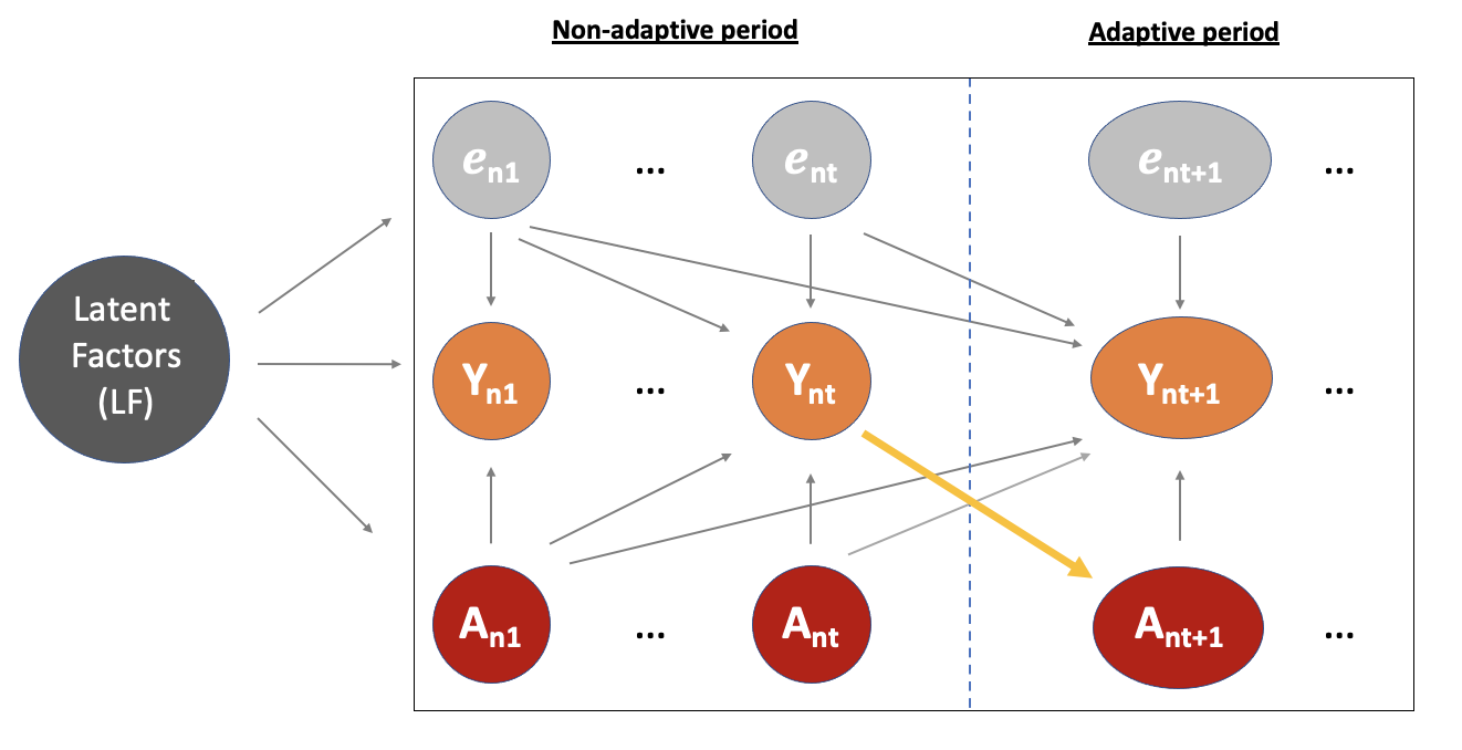
Figure 2: DAG that is consistent with the exogeneity conditions implied by the definition of $\mathcal{I}^{a}_{t}$. From time step $t+1$, the action sequence$[A_{n,t+1},\dots,A_{n,T}]$ can be adaptive, i.e., dependent on the observed outcomes $[Y_{n,t}]_{t\in[T]}$.

Overcoming limitations of LTV identification strategy. We see this additional linear time-varying latent factor structure, motivated by a linear time-varying dynamical system, buys us a lot in terms of the number of donor units required and how adaptive their action sequence can be. This begs the question how much more can be gained if we instead had a linear time-invariant latent factor structure, motivated by linear time-invariant dynamical system. In Section 5, we show this additional structure surprisingly implies far better donor sample complexity and less stringent exogeneity conditions on these donor units.

5 Linear Time-Invariant Latent Factor Model

Below we introduce a linear time-invariant factor model which is analogous to the factor model introduced in Assumption 4.

Assumption 7 (Linear time-invariant (LTI) factor model).

Assume $\forall\ n\in[N]$, $t\in[T],\bar{a}^{t}\in[\mathcal{A}]^{t}$,

$$Y^{(\bar{a}^{t})}_{n,t} =\sum^{t}_{\ell=1}\left\langle\psi^{t-\ell}_{n},w_{a_{\ell}}\right\rangle+\varepsilon^{(\bar{a}^{t})}_{n,t}.$$ (13)

where $\psi^{t-\ell}_{n},w_{a_{\ell}}\in\mathbb{R}^{d}$ for $\ell\in[t]$. Further, let $\mathcal{LF}=\{\psi^{t-\ell}_{n}\}_{n\in[N],t\in[T],\ell\in[0,t-1]}\cup\{w_{a}\}_{a\in[\mathcal{A}]}$. Assume,

$$\mathbb{E}[\varepsilon^{(\bar{a}^{t})}_{n,t}\mid\mathcal{LF}]=0$$ (14)

Remark.

Note Assumption 7 implies Assumption 2 holds with

$$v_{n,t}=[\psi^{t-1}_{n},\dots,\psi^{t-t}_{n}],\ w_{\bar{a}^{t}}=[w_{a_{1}},\dots,w_{a_{t}}].$$

Further $d(t)=d\times t$ for $d(t)$ in Definition 1.

We see that the effect of action $a_{\ell}$ on $Y^{(\bar{a}^{t})}_{n,t}$ for $\ell\in[t]$ is additive, given by $\langle\psi^{t-\ell}_{n},w_{a_{\ell}}\rangle$. Intuitively, $\psi_{n}^{t-\ell}$ captures the latent unit specific heterogeneity in the potential outcome for unit $n$, at a given time step $t$, for an action taken at time step $\ell\leq t$; analogously $w_{a_{\ell}}$ captures the latent effect of action $a_{\ell}$. Further, compared to Assumption 4, we now have the additional structure that rather than being dependent on the specific time steps $\ell$ and $t$, $\psi^{t-\ell}_{n}$ is only dependent on the lag $t-\ell$. As a result, the effect of action taken at time $\ell$ on the outcome at time $t$ is only a function of the lag $t-\ell$. Hence we call this a “time-invariant” latent factor model, as opposed to a “time-varying” latent factor model. This additional structure along will be crucial in the identification strategy we employ in Section 5.2.

Non-varying control sequence. For this identification strategy, we make the additional assumption that the control sequence is also time invariant.

Assumption 8.

There exists $\tilde{0}\in[\mathcal{A}]$ such that the control sequence $0_{t}=\tilde{0}$ for all $t\in[T]$.

5.1 Motivating Example

We show that the classical linear time-varying dynamical system model satisfies Assumption 2. Suppose for all $t\in[T]$, all units $n\in[N]$ obey the following dynamical system for a sequence of actions $\bar{A}^{t}_{n}$ (assume $z_{n,0},w_{A_{n,0}}=0$):

$$A_{n,t} =f_{n}(w_{A_{n,t-1}},\ z^{(\bar{A}_{n}^{t-1})}_{n,t-1}),$$

$$z^{(\bar{A}_{n}^{t})}_{n,t} =\boldsymbol{B}_{n}\ z^{(\bar{A}_{n}^{t-1})}_{n,t-1}+\boldsymbol{C}_{n}\ w_{A_{n,t}}+\eta_{n,t}$$

$$Y^{(\bar{A}_{n}^{t})}_{n,t} =\left\langle\theta_{n},z^{(\bar{A}_{n}^{t})}_{n,t}\right\rangle+\left\langle\tilde{\theta}_{n},w_{A_{n,t}}\right\rangle+\tilde{\eta}_{n,t}.$$

Here, $z^{(\bar{A}_{n}^{t})}_{n,t}\in\mathbb{R}^{d}$ is the latent state associated with unit $n$ at time $t$ and $w_{A_{n,t-1}}\in\mathbb{R}^{d}$ is the chosen action at time $t-1$. $\eta_{n,t}\in\mathbb{R}^{d}$ and $\tilde{\eta}_{n,t}\in\mathbb{R}$ represent independent mean-zero random innovations at each time step $t$. $\boldsymbol{B}_{n},\boldsymbol{C}_{n}\in\mathbb{R}^{d\times d}$ are matrices governing the linear dynamics of $z^{(\bar{A}_{n}^{t})}_{n,t}$. In contrast, in the linear time-varying dynamical system described in Section 4.1 above, these transition matrices are invariant across all $t\in[T]$. $\theta_{n},\tilde{\theta}_{n}\in\mathbb{R}^{d}$ are parameters governing how the outcome of interest $Y^{(\bar{A}_{n}^{t})}_{n,t}$ is a linear function of $z^{(\bar{A}_{n}^{t})}_{n,t}$ and $w_{a_{t}}$, respectively. $f_{n}(\cdot)$ is a function which decides how the next action $w_{A_{n,t}}$ is chosen as a function of the previous action $w_{A_{n,t-1}}$, and current state $z^{(\bar{A}_{n}^{t})}_{n,t}$. We see that due to the input of $z^{(\bar{A}_{n}^{t})}_{n,t}$ in $f_{n}(\cdot)$, i.e., the action sequence is adaptive. As a result, $\eta_{n,\ell}$ is correlated with $A_{n,t}$ for $\ell<t$.

Proposition 3.

Suppose the linear time-varying dynamical system above holds. Assume $z_{n,0},\ w_{a_{0}}=0$. Then we have the following representation,

$$Y^{(\bar{a}^{t})}_{n,t}=\sum^{t}_{\ell=1}\Big{(}\left\langle\psi^{t-\ell}_{n},w_{a_{\ell}}\right\rangle+\varepsilon_{n,t,\ell}\Big{)},$$ (15)

where $\psi^{t,\ell}_{n},w_{a_{\ell}}\in\mathbb{R}^{d}$ for $\ell\in[t]$; here,

$$\psi^{t-\ell}_{n} =\left(\boldsymbol{B}^{t-\ell}_{n}\boldsymbol{C}_{n}\right)^{\prime}\theta_{n}\quad\text{for}\quad\ell\in[t-1],$$

$$\psi^{0}_{n} =(\boldsymbol{C}_{n})^{\prime}\theta_{n}+\tilde{\theta_{n}},$$

$$\varepsilon_{n,t,\ell} =\left(\boldsymbol{B}^{t-\ell}_{n}\eta_{n,\ell}\right)^{\prime}\theta_{n}\quad\text{for}\quad\ell\in[t-1],$$

$$\varepsilon_{n,t,t} =\left(\eta_{n,t}\right)^{\prime}\theta_{n}+\tilde{\eta}_{n,t}.$$

Therefore, Assumption 7 holds with the additional structure that $\varepsilon^{(\bar{a}^{t})}_{n,t}$ has an additive factorization as $\sum^{t}_{\ell=1}\varepsilon_{n,t,\ell}$, and it is not a function of $a_{\ell}$.

In this example, our target parameter $\mathbb{E}[Y^{(\bar{a}^{T})}_{n,T}~{}|~{}\mathcal{LF}]$ defined in (target causal parameter) translates to the expected potential once we condition on the latent parameters $\psi^{t,\ell}_{n},w_{a_{\ell}}$, which are a function of $\boldsymbol{B}_{n},\boldsymbol{C}_{n},\theta_{n},\tilde{\theta}_{n}$, and we take the average over the per-step independent mean-zero random innovations, $\varepsilon_{n,t,\ell}$, which is a function of $\eta_{n,\ell}$ (and $\boldsymbol{B}_{n},\boldsymbol{C}_{n},\theta_{n}$).

Note that once we re-write this linear time-varying dynamical system in terms of the latent factor representation, we do not need to observe the parameters $z^{(\bar{A}_{n}^{t})}_{n,t}$ and $w_{a_{\ell}}$ to express the potential outcomes in terms of them. The only information we need about $w_{a_{\ell}}$ is a unique identifier, given by $a_{\ell}$. Traditionally, state-based models of linear dynamical systems literature require that both $z^{(\bar{A}_{n}^{t})}_{n,t}$ and $w_{a_{\ell}}$ are perfectly observed. Input-output models for dynamical systems assume that $w_{a_{\ell}}$ is perfectly observed.

5.2 Identification Strategy

Recall out goal in this section is to identify $\mathbb{E}[Y_{n,T}^{(\bar{a}^{T})}\mid\mathcal{LF}]$, i.e., represent this expected potential outcome for a target unit $n$ and action sequence $\bar{a}^{T}$ as some function of observed outcomes.

5.2.1 Notation and Assumptions

Notation. We define the following useful notation for any unit $n\in[N]$ and $t\in[T]$:

$$\gamma_{n,T-t}(a):=\left\langle\psi^{T-t}_{n},w_{a}-w_{\tilde{0}}\right\rangle$$

$\gamma_{n,T-t}(a)$ can be interpreted as a “blip effect”, i.e., the expected difference in potential outcomes if unit $n$ undergoes the sequence $(\bar{a}^{T-t},\underline{0}^{T-t+1})$ instead of $(\bar{a}^{T-t-1},\underline{0}^{T-t})$. That is, Assumption 7 and 8 imply

$$\mathbb{E}\left[Y^{(\bar{a}^{T-t},\underline{0}^{T-t+1})}_{n,T}-Y^{(\bar{a}^{T-t-1},\underline{0}^{T-t})}_{n,T}\mid\mathcal{LF}\right] =\mathbb{E}\left[\left\langle\psi^{T-t}_{n},w_{a_{t}}-w_{\tilde{0}}\right\rangle+\varepsilon^{(\bar{a}^{T-t},\underline{0}^{T-t+1})}_{n,T}-\varepsilon^{(\bar{a}^{T-t-1},\underline{0}^{T-t})}_{n,T}\mid\mathcal{LF}\right]$$

$$=\left\langle\psi^{T-t}_{n},w_{a_{t}}-w_{\tilde{0}}\right\rangle\mid\mathcal{LF}.$$

Further, let

$$b_{n,t} :=\sum^{t}_{\ell=1}\left\langle\psi^{t-\ell}_{n},w_{\tilde{0}}\right\rangle.$$

This can be interpreted as the expected potential outcome if unit $j$ remains under the control sequence $\bar{0}^{T}$ till time step $T$. Again, Assumption 7 and 8 imply

$$\mathbb{E}\left[Y^{(\bar{0}^{T})}_{n,T}\mid\mathcal{LF}\right] =\mathbb{E}\left[\sum^{T}_{t=1}\left\langle\psi^{T,t}_{n},w_{\tilde{0}}\right\rangle+\varepsilon^{(\bar{0}^{T})}_{n,t}\mid\mathcal{LF}\right]=\sum^{T}_{t=1}\left\langle\psi^{T,t}_{n},w_{\tilde{0}}\right\rangle\mid\mathcal{LF}$$ (16)

Assumptions. We now state the various assumptions we need for the identification strategy that we propose next.

Donor sets. We define different subsets of units based on the action sequence they receive.

$$\mathcal{I}^{a}\coloneqq\{j\in[N]: \ (i)\ \bar{A}^{t^{*}_{j}}_{j}=(\tilde{0},\dots,\tilde{0},a),$$

$$(ii)\ \forall\ \bar{\alpha}^{t}\in[\mathcal{A}]^{t},t\in[T],\ \mathbb{E}[Y^{(\bar{\alpha}^{t})}_{j,t}\mid\mathcal{LF},\bar{A}^{t^{*}_{j}}_{j}]=\mathbb{E}[Y^{(\bar{\alpha}^{t})}_{j,t}\mid\mathcal{LF}]\},$$ (17)

$$\mathcal{I}^{0}_{t}\coloneqq\{j\in[N]: \ (i)\ \bar{A}^{t}_{j}=(\tilde{0},\dots,\tilde{0}),$$

$$(ii)\ \forall\ \alpha^{\ell}\in[\mathcal{A}]^{\ell},\ell\in[T],\ \mathbb{E}[Y^{(\bar{\alpha}^{\ell})}_{j,\ell}\mid\mathcal{LF},\bar{A}^{t}_{j}]=\mathbb{E}[Y^{(\bar{\alpha}^{\ell})}_{j,\ell}\mid\mathcal{LF}]\},$$ (18)

$\mathcal{I}^{a}$ refers to units that remain under the control sequence $(\tilde{0},\dots,\tilde{0})$ till time step $t^{*}_{j}-1$, and at time step $t^{*}_{j}$ receive action $a$. Further, we require that for these particular units, the action sequence, $\bar{A}^{t^{*}_{j}}_{j}$, till time step $t^{*}_{j}$ was chosen such that $\mathbb{E}[Y^{(\bar{\alpha}^{t})}_{j,t}\mid\mathcal{LF},\bar{A}^{t^{*}_{j}}_{j}]=\mathbb{E}[Y^{(\bar{\alpha}^{t})}_{j,t}\mid\mathcal{LF}]$ for all $\bar{\alpha}^{t}\in[\mathcal{A}]^{t}$, i.e., the potential outcomes are conditionally mean independent of the action sequence $\bar{A}^{t^{*}_{j}}_{j}$ unit $j$ receives till time step $t^{*}_{j}$. Of course, a sufficient condition for property (ii) above is that $\forall\ \bar{\alpha}^{t}\in[\mathcal{A}]^{t},\ \ Y^{(\bar{\alpha}^{t})}_{j,t}\perp\bar{A}^{t^{*}_{j}}_{j}\mid\mathcal{LF}$. That is, for these units, the action sequence till time step $t^{*}_{j}$ is chosen at $t=0$ conditional on the latent factors, i.e., the policy for these units can only be adaptive from time step $t^{*}_{j}+1$. Note, given Assumption 7, (17) can be equivalently stated as $\mathbb{E}[\varepsilon^{(\bar{\alpha}^{t})}_{j,t}\mid\mathcal{LF},\bar{A}^{t^{*}_{j}}_{j}]=\mathbb{E}[\varepsilon^{(\bar{\alpha}^{t})}_{j,t}\mid\mathcal{LF}]=0$. $\mathcal{I}^{0}_{t}$ follows a similar intuition to that of $\mathcal{I}^{a}$.

Assumption 9.

For $n\in[N]$, let $v_{n,T}:=[\psi^{0}_{n},\dots,\psi^{T-1}_{n}]$. We assume that for all $n\in[N]$, $v_{n,T}$ satisfies a well-supported condition with respect to the various donor sets, i.e., for all $a\in[\mathcal{A}]$ there exists $\beta^{n,\mathcal{I}^{a}}\in\mathbb{R}^{|\mathcal{I}^{a}|}$, and $\beta^{n,\mathcal{I}^{0}_{t}}\in\mathbb{R}^{|\mathcal{I}^{0}_{t}|}$ such that

$$v_{n,T}=\sum_{k\in\mathcal{I}^{a}}\beta_{k}^{n,\mathcal{I}^{a}}v_{k,T},\quad v_{n,T}=\sum_{k\in\mathcal{I}^{0}_{t}}\beta_{k}^{n,\mathcal{I}^{0}_{t}}v_{k,T}$$ (LTI well-supported factors)

Assumption 9 essentially states that for the various units $n\in[N]$, their latent factors $[\psi^{T-1}_{n},\dots,\psi^{T-T}_{n}]$ are expressible as a linear combination of the units in the donor sets $\mathcal{I}^{a}$ and $\mathcal{I}^{0}_{t}$. See the discussion under Assumption 3 in Section 3 justifying such an assumption for settings when $\mathcal{I}^{a},\mathcal{I}^{0}_{t}$ is sufficiently large.

Assumption 10.

For all $n\in[N],t\in[T]$, $\bar{\alpha}^{t}\in[\mathcal{A}]^{t}$,

$$\mathbb{E}\left[\varepsilon_{n,t}^{(\bar{\alpha}^{t})}-\varepsilon_{n,t}^{(\bar{\alpha}^{t-1},\tilde{0})}\mid\bar{A}^{t}_{n}=\bar{\alpha}^{t},\ \mathcal{LF}\right]=0.$$ (19)

For sufficient conditions under which Assumption 10 holds, see the discussion under Assumption 6 in Section 4.2—an analogous argument holds here. Also an analogous version of Proposition 2 holds for the linear time-invariant setting using an identical argument.

5.2.2 Identification Result

Given these assumptions, we now present our identification theorem.

Theorem 3.

Let Assumptions 1, 7, 8, 9, and 10 hold. Then, for any unit $n\in[N]$ and action sequence $\bar{a}^{T}\in[\mathcal{A}]^{T}$, the expected counterfactual outcome can be expressed as:

$$\mathbb{E}[Y_{n,T}^{(\bar{a}^{T})}\mid\mathcal{LF}]=~{} \sum_{t=1}^{T}\gamma_{n,T-t}(a_{t})+b_{n,T}\mid\mathcal{LF}.$$ (identification)

We have the following representations of the baseline outcomes for all $t\in[T]$

$$\forall\ j\in\mathcal{I}^{0}_{t}~{}:~{}b_{j,t}\mid\mathcal{LF}=\mathbb{E}[Y_{j,t}\mid\mathcal{LF},\ j\in\mathcal{I}^{0}_{t}],$$ (observed control)

$$\forall\ i\notin\mathcal{I}^{0}_{t}~{}:~{}b_{i,t}\mid\mathcal{LF}=\sum_{j\in\mathcal{I}^{0}_{t}}\beta_{j}^{i,\mathcal{I}^{0}_{t}}\ b_{j,t}\mid\mathcal{LF},\mathcal{I}^{0}_{T}.$$ (synthetic control)

We have the following representations of the blip effect with $0$ lag, for $\forall a\in[\mathcal{A}]$:

$$\forall\ j\in\mathcal{I}^{a}~{}:~{} \gamma_{j,0}(a)\mid\mathcal{LF}=~{}\mathbb{E}[Y_{j,t^{*}_{j}}\mid\mathcal{LF},\ j\in\mathcal{I}^{a}]-b_{j,t^{*}_{j}}\mid\mathcal{LF}, 0$$ (observed lag blip)

$$\forall\ i\notin\mathcal{I}^{a}~{}:~{} \gamma_{i,0}(a)\mid\mathcal{LF}=~{}\sum_{j\in\mathcal{I}^{a}}\beta_{j}^{i,\mathcal{I}^{a}}\gamma_{j,0}(a)\mid\mathcal{LF},\mathcal{I}^{a}. 0$$ (synthetic lag blip)

We have the following recursive representations of the blip effect $\forall\ t\in[T-1],\ a\in[\mathcal{A}]$:

$$\forall\ j\in\mathcal{I}^{a} ~{}:~{}\gamma_{j,t}(a)\mid\mathcal{LF}=~{}\mathbb{E}[Y_{j,t^{*}_{j}+t}\mid\mathcal{LF},\mathcal{I}^{a}]-b_{j,t^{*}_{j}+t}\mid\mathcal{LF}-\sum^{t-1}_{\ell=0}\gamma_{j,\ell}(A_{j,t^{*}_{j}+t-\ell})\mid\mathcal{LF}, t$$ (observed lag blip)

$$\forall\ i\notin\mathcal{I}^{a} ~{}:~{}\gamma_{i,t}(a)\mid\mathcal{LF}=~{}\sum_{j\in\mathcal{I}^{a}}\beta_{j}^{i,\mathcal{I}^{a}}\gamma_{j,t}(a)\mid\mathcal{LF},\mathcal{I}^{a}. t$$ (synthetic lag blip)

Interpretation of identification result. (identification) states that our target causal parameter of interest can be written as an additive function of $b_{n,T}$ and $\gamma_{n,T-t}(a_{t})$ for $t\in[T]$ and $a_{t}\in[\mathcal{A}]$. Theorem 3 establishes that these various quantities are expressible as functions of observed outcomes$\{Y_{j,t}\}_{j\in[N],t\in[T]}$. We give an interpretation below.

Identifying baseline outcomes. Similar to the intuition for Theorem 2, for units $j\in\mathcal{I}^{0}_{t}$, (observed control) states that their baseline outcome $b_{j,t}$ is simply their expected observed outcome at time step $t$, i.e., $Y_{j,t}$. For units $i\notin\mathcal{I}^{0}_{t}$, (synthetic control) states that we can identify $b_{i,t}$ by appropriately re-weighting the baseline outcomes $b_{j,t}$ of the units $j\in\mathcal{I}_{t}^{0}$ (identified via (observed control)).

Identifying blip effects for lag $0$. For any given $a\in[\mathcal{A}]$: For units $j\in\mathcal{I}^{a}$, (observed lag $0$ blip) states that their blip effect $\gamma_{j,0}(a)$ is equal to their observed outcome $Y_{j,t^{*}_{j}}$ minus the baseline outcome $b_{j,t^{*}_{j}}$ (identified via (synthetic control)). Recall $t^{*}_{j}$ is equal to the first time step that unit $j$ is no longer in the control sequence. For units $i\notin\mathcal{I}^{a}$, (synthetic lag $0$ blip) states that we can identify $\gamma_{i,0}(a)$ by appropriately re-weighting the blip effects $\gamma_{j,0}(a)$ of units $j\in\mathcal{I}^{a}$ (identified via (observed lag $0$ blip)).

Identifying blip effects for lag $t$ with $t\in[T-1]$. Suppose by induction $\gamma_{n,\ell}(a)$ is identified for every lag $\ell<t$, $n\in[N]$, $a\in[\mathcal{A}]$, i.e., can be expressed in terms of observed outcomes. Then for any given $a\in[\mathcal{A}]$: For units $j\in\mathcal{I}^{a}$, (observed lag $t$ blip) states that their blip effect $\gamma_{j,t}(a)$ is equal to their their observed outcome at time step $t^{*}_{j}+t$, $Y_{j,t^{*}_{j}+t}$, minus the baseline outcome $b_{j,t^{*}_{j}+t}$ (identified via (synthetic control)) minus the sum of blip effects for smaller lags, $\sum_{\ell=0}^{t-1}\gamma_{j,\ell}(A_{j,t^{*}_{j}+t-\ell})$ (identified via the inductive hypothesis). For units $i\notin\mathcal{I}^{a}$, (synthetic lag $t$ blip) states that we can identify $\gamma_{i,t}(a)$ by appropriately re-weighting the blip effects $\gamma_{j,t}(a)$ of units $j\in\mathcal{I}^{a}$ (identified via (observed lag $t$ blip)).

5.3 Synthetic Blip Effects Algorithm - LTI Setting

We now show how the identification strategy laid out above naturally leads to an estimation algorithm. For this section, we assume we have oracle knowledge of $\beta^{n,\mathcal{I}^{a}}\in\mathbb{R}^{|\mathcal{I}^{a}|},\ \beta^{n,\mathcal{I}^{0}_{t}}\in\mathbb{R}^{|\mathcal{I}^{0}_{t}|}$ for $n\in[N]$, $a\in[\mathcal{A}],t\in[T]$. Refer to Appendix A for how to estimate $\beta^{n,\mathcal{I}^{a}},\beta^{n,\mathcal{I}^{0}_{t}}$.

Step 1: Estimate baseline outcomes.

For $t\in[T]$:

1. For $j\in\mathcal{I}^{0}_{t}$

   $$\hat{b}_{j,t}=Y_{j,t}$$

2. For $i\notin\mathcal{I}^{0}_{t}$

   $$\hat{b}_{i,t}=\sum_{j\in\mathcal{I}^{0}_{t}}\beta_{j}^{i,\mathcal{I}^{0}_{t}}Y_{j,t}$$

Step 2: Estimate blip effects for lag $0$.

For $a\in[\mathcal{A}]$:

1. For $j\in\mathcal{I}^{a}$

   $$\hat{\gamma}_{j,0}(a)=Y_{j,t^{*}_{j}}-\hat{b}_{j,t^{*}_{j}}$$

2. For $i\notin\mathcal{I}^{a}$

   $$\hat{\gamma}_{i,0}(a)=\sum_{j\in\mathcal{I}^{a}}\beta_{j}^{i,\mathcal{I}^{a}}\hat{\gamma}_{j,0}(a)$$

Step 3: Recursively estimate blip effects for time $t<T$.

For $a\in[\mathcal{A}]$ and $t\in\{1\dots,T-1\}$, recursively estimate as follows:

1. For $j\in\mathcal{I}^{a}$

   $$\hat{\gamma}_{j,t}(a)=Y_{j,t^{*}_{j}+t}-\hat{b}_{j,t^{*}_{j}+t}-\sum_{\ell=0}^{t-1}\hat{\gamma}_{j,\ell}(A_{n,t^{*}_{j}+t-\ell})$$

2. For $i\notin\mathcal{I}^{a}$

   $$\hat{\gamma}_{i,t}(a)=\sum_{j\in\mathcal{I}^{a}}\beta_{j}^{i,\mathcal{I}^{a}}\hat{\gamma}_{j,t}(a)$$

Step 4: Estimate target causal parameter. For $n\in[N]$, and $\bar{a}^{T}\in[\mathcal{A}]^{T}$, estimate the causal parameter as follows:

$$\widehat{\mathbb{E}}[Y_{n,T}^{(\bar{a}^{T})}\mid\mathcal{LF}]=~{} \sum_{t=1}^{T}\hat{\gamma}_{n,T-t}(a_{t})+\hat{b}_{n,T}.$$ (20)

5.3.1 LTV Identification Strategy: Donor Sample Complexity & Exogeneity Conditions

Donor sample complexity. To estimate $\mathbb{E}[Y^{(\bar{a}^{T})}_{n,T}~{}|~{}\mathcal{LF}]$ for all units $n\in[N]$ and any action sequence $\bar{a}^{T}\in[\mathcal{A}]^{T}$, the LTI identification strategy requires the existence of a sufficiently large subset of donor units $\mathcal{I}^{a}$ for every $a\in[\mathcal{A}]$ and $\mathcal{I}^{0}_{t}$ for $t\in[T]$. That is, the number of donor units we require will need to scale at the order of $|\mathcal{A}|$ to ensure sufficient number of units for the donor sets $\{\mathcal{I}^{a}\}_{a\in|\mathcal{A}|}$. To ensure that we have sufficient number of donors units for $\mathcal{I}^{0}_{t}$ for $t\in[T]$. But notice from the definition of $\mathcal{I}^{0}_{t}$ that for all $t\in[T-1]$, $\mathcal{I}^{0}_{t}\subset\mathcal{I}^{0}_{T}$. Hence, we just require that $\mathcal{I}^{0}_{T}$ is sufficiently large. As a result the total donor sample complexity needs to scale at the order of $|\mathcal{A}|+1$. Thus we see the the additional structure imposed by the time-invariant factor model introduced in Assumption 7 leads to a decrease in sample complexity from $|\mathcal{A}|\times T$ to $|\mathcal{A}|+1$, when compared with the time-varying factor model factor model introduced in Assumption 4. The other major assumption made is that the control sequence is also not time varying, see Assumption 8.

Donor exogeneity conditions. Further, for $j\in\mathcal{I}^{a}$, we require that $\forall\ \bar{\alpha}^{t}\in[\mathcal{A}]^{t},t\in[T],\ \mathbb{E}[Y^{(\bar{\alpha}^{t})}_{j,t}\mid\mathcal{LF},\bar{A}^{t^{*}_{j}}_{j}]=\mathbb{E}[Y^{(\bar{\alpha}^{t})}_{j,t}\mid\mathcal{LF}]$. That is, the actions picked for these donor units are only required to be non-adaptive till time step $t^{*}_{j}$. As a special case, if we restrict ourselves to units

$$\tilde{\mathcal{I}}^{a}\coloneqq\{j\in\mathcal{I}^{a}:t^{*}_{j}=1\},$$ (21)

then we actually impose no exogeneity conditions. That is, for these donor units, their entire action sequence can be adaptive. In contrast for the identification strategy in Section 4, we require that the donor units in $\mathcal{I}^{a}_{t}$ are non-adaptive till time step $t$. See Figure 3 for a DAG that is consistent with the exogeneity conditions implied by the definition of $\tilde{\mathcal{I}}^{a}$ in (8).

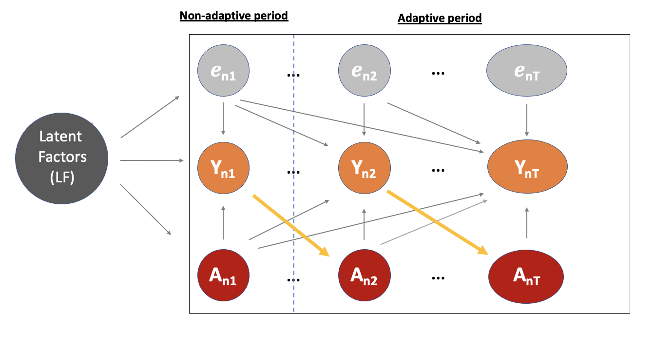
Figure 3: DAG that is consistent with the exogeneity conditions implied by the definition of $\tilde{\mathcal{I}}^{a}$. From time step $2$, the action sequence$[A_{n,2},\dots,A_{n,T}]$ can be adaptive, i.e., dependent on the observed outcomes $[Y_{n,t}]_{t\in[T]}$. Hence, there is no non-adaptive period for these units

6 Conclusion

In this work, we formulate a causal framework for linear dynamical systems, a popular model in across many fields to study dynamics. We propose a latent factor model, which admits linear time-varying and time-invariant dynamical systems as special cases. Depending on the structure placed on this factor model, we quantify the trade-off on the sample complexity and the level of adaptivity allowed in the intervention policy, for estimating counterfactual mean outcomes. We hope this work spurs further research connecting the growing fields of synthetic controls and panel data methods with dynamic treatment models studied in econometrics, and potentially sequential learning methods such as reinforcement learning studied in computer science.

Appendix A Computing Linear Weights

The estimation algorithms in Sections 4.3 and 5.3 assume oracle knowledge of the linear weights $\beta^{n,\mathcal{I}}$ such that the latent unit factor for unit $n$ can be written as a linear combination of the latent factors $\{v_{j}\}_{j\in\mathcal{I}}$, where $\mathcal{I}$ is the relevant donor set. Recall, in Section 4.3, the donor sets are of the form $\mathcal{I}^{a}_{t}$ for $a\in[\mathcal{A}],t\in[T]$; in Section 5.3 they are of the form $\mathcal{I}^{a}$ for $a\in[\mathcal{A}]$ (and $\mathcal{I}^{0}_{t}$ for $t\in[T]$).

We now discuss how these linear weights can be estimated from data. To do so, we make an additional assumption that we have access to covariates for each unit that also have a latent factorization.

Assumption 11.

For each unit $n\in[N]$, we assume access to covariates $X_{n}\in\mathbb{R}^{p}$ such that

$$X_{nj}=\left\langle v_{n,T},\rho_{j}\right\rangle+\varepsilon_{nj},$$ (22)

where $v_{n,T}$ is the unit latent factor defined in Assumption 2, 4 and 7. And $\varepsilon_{nj}$ is mean-zero noise.

Note that if $\min_{n\in[N]}t^{*}_{n}=p$, then we can take $X_{n}$ to be the observations of the various units under the control sequence. That is, $X_{nj}=Y_{nj}$ for $j\in\min_{n\in[N]}$. In this case $\rho_{j}=w_{0_{j}}$, the latent factor associated with the control action at time $j$. However, Assumption 11 also allows for access to auxiliary covariates, as long as they share the same latent factor structure.

A.1 Linear Weight Estimation Algorithm

Below, we detail the algorithm to estimate $\beta^{n,\mathcal{I}}$. Define $\boldsymbol{X}=[X_{ij}]_{i\in[N],j\in\mathcal{I}}\in\mathbb{R}^{|\mathcal{I}|\times p}$. Let $\boldsymbol{X}^{\prime}$ be the transpose of $\boldsymbol{X}$. Define the singular value decomposition (SVD) of $\boldsymbol{X}^{\prime}$ as follows:

$$\boldsymbol{X}^{\prime}=\sum^{\min(n,\mathcal{I})}_{\ell=1}\sigma_{\ell}u_{\ell}v^{\prime}_{\ell},$$ (23)

where the singular values $\sigma_{\ell}$ are ordered by magnitude and $u_{\ell}\in\mathbb{R}^{p},v^{\prime}_{\ell}\in\mathbb{R}^{|\mathcal{I}|}$ are the associated left and right singular vectors of $\boldsymbol{X}^{\prime}$. Then $\beta^{n,\mathcal{I}}$ can be estimated via principal component regression (PCR). Specifically, with $k\in\min(n,\mathcal{I})$ is a hyper-parameter,

$$\widehat{\beta}^{n,\mathcal{I}}=\Big{(}\sum^{k}_{\ell=1}(\sigma_{\ell})^{-1}v_{j\ell}u_{i\ell}\Big{)}X^{\prime}_{n}$$ (24)

For justification of why to use PCR in this setting, refer to Agarwal et al., 2021b ; Agarwal et al., 2020a .

Appendix B Connection to SNMM and MSM - Proof of Proposition 2

Verifying Assumption  4 holds. In what follows, all the conditional expectations are also conditioned on the latent factors $\mathcal{LF}$. However, for shorthand notation, we omit that conditioning. Note that:

$$\mathbb{E}\left[Y_{n,t}^{(\bar{a}^{t})}-Y_{n,t}^{(\bar{0}_{t})}\right]=~{} \sum_{\ell=1}^{t}\mathbb{E}\left[Y_{n,t}^{(\bar{a}^{\ell},\underline{0}^{\ell+1})}-Y_{n,t}^{(\bar{a}^{\ell-1},\underline{0}^{\ell})}\right]$$ (25)

We now prove that:

$$Q_{n,t}\coloneqq\mathbb{E}\left[Y_{n,t}^{(\bar{a}^{\ell},\underline{0}^{\ell+1})}-Y_{n,t}^{(\bar{a}^{\ell-1},\underline{0}^{\ell})}\right]=\left\langle\psi_{n}^{t,\ell},w_{a^{\ell}}-w_{0^{\ell}}\right\rangle$$

We establish this via a nested mean argument. Note

$$Q_{n,t}=~{} \mathbb{E}\left[\mathbb{E}\left[Y_{n,t}^{(\bar{a}_{n}^{\ell},\underline{0}^{\ell+1})}-Y_{n,t}^{(\bar{a}_{n}^{\ell-1},\underline{0}^{\ell})}\mid S_{n}^{0}\right]\right]$$

$$=~{} \mathbb{E}\left[\mathbb{E}\left[Y_{n,t}^{(\bar{a}_{n}^{\ell},\underline{0}^{\ell+1})}-Y_{n,t}^{(\bar{a}_{n}^{\ell-1},\underline{0}^{\ell})}\mid S_{n}^{0},A_{n}^{1}=a^{1}\right]\right]$$ (26)

where in (26), we have used (9). Now as our inductive step, suppose that we have shown:

$$Q_{n,t}=~{} \mathbb{E}\left[\mathbb{E}\left[\ldots\mathbb{E}\left[Y_{n,t}^{(\bar{a}^{\ell},\underline{0}^{\ell+1})}-Y_{n,t}^{(\bar{a}^{\ell-1},\underline{0}^{\ell})}\mid\bar{S}_{n}^{q-1},\bar{A}_{n}^{q}=\bar{a}^{q}\right]\ldots\mid S_{n}^{0},A_{n}^{1}=a^{1}\right]\right]$$

Then,

$$Q_{n,t}=~{} \mathbb{E}\left[\mathbb{E}\left[\ldots\mathbb{E}\left[\mathbb{E}\left[Y_{n,t}^{(\bar{a}^{\ell},\underline{0}^{\ell+1})}-Y_{n,t}^{(\bar{a}^{\ell-1},\underline{0}^{\ell})}\mid\bar{S}_{n}^{q},\bar{A}_{n}^{q}=\bar{a}^{q}\right]\mid\bar{S}_{n}^{q-1},\bar{A}_{n}^{q}=\bar{a}^{q}\right]\ldots\mid S_{n}^{0},A_{n}^{1}=a^{1}\right]\right]$$

$$=~{} \mathbb{E}\left[\mathbb{E}\left[\ldots\mathbb{E}\left[\mathbb{E}\left[Y_{n,t}^{(\bar{a}^{\ell},\underline{0}^{\ell+1})}-Y_{n,t}^{(\bar{a}^{\ell-1},\underline{0}^{\ell})}\mid\bar{S}_{n}^{q},\bar{A}_{n}^{q+1}=\bar{a}^{q+1}\right]\mid\bar{S}_{n}^{q-1},\bar{A}_{n}^{q}=\bar{a}^{q}\right]\ldots\mid S_{n}^{0},A_{n}^{1}=a^{1}\right]\right],$$ (27)

where in (27), we have again used (9). This concludes the inductive proof. Thus, we have

$$Q_{n,t}=~{} \mathbb{E}\left[\mathbb{E}\left[\ldots\mathbb{E}\left[Y_{n,t}^{(\bar{a}^{\ell},\underline{0}^{\ell+1})}-Y_{n,t}^{(\bar{a}^{\ell-1},\underline{0}^{\ell})}\mid\bar{S}_{n}^{\ell-1},\bar{A}_{n}^{\ell}=\bar{a}^{\ell}\right]\ldots\mid S_{n}^{0},A_{n}^{1}=a^{1}\right]\right]$$

$$=~{} \mathbb{E}\left[\mathbb{E}\left[\ldots\gamma_{n,t,\ell}(a^{\ell})\ldots\mid S_{n}^{0},A_{n}^{1}=a^{1}\right]\right]=\left\langle\psi_{n}^{t,\ell},w_{a^{\ell}}-w_{0^{\ell}}\right\rangle$$ (28)

where in (28), we have used (10) and the fact that $\left\langle\psi_{n}^{t,\ell},w_{a^{\ell}}-w_{0^{\ell}}\right\rangle$ is independent of $S^{\ell}_{n}$ and $\bar{A}^{\ell-1}_{n}$. Re-arranging (25) and (28), we have:

$$\mathbb{E}\left[Y_{n,t}^{(\bar{a}^{t})}\right]=\mathbb{E}\left[Y_{n,t}^{(\bar{0}^{t})}\right]+\sum_{\ell=1}^{t}\gamma_{n,t,\ell}({a}^{\ell}).$$ (29)

Combining (29) and (11) implies Assumption 4 holds.

Verifying Assumption  6 holds. Assumption 6 is immediately implied by (10) and a simple application of the tower law of expectations. In particular, we integrate $\bar{S}_{n,t-1}$ out of both sides of (10).

Appendix C Proof of Theorem 1

By Assumption 2,

$$\mathbb{E}\left[Y_{n,T}^{(\bar{a}^{T})}\mid\mathcal{LF}\right] =\mathbb{E}\left[\left\langle v_{n,T},\ w_{\bar{a}^{T}}\right\rangle+\varepsilon^{(\bar{a}^{T})}_{n,t}\mid\mathcal{LF}\right]$$

$$=\mathbb{E}\left[\left\langle v_{n,T},\ w_{\bar{a}^{T}}\right\rangle\mid\mathcal{LF}\right]$$

$$=\left\langle v_{n,T},\ w_{\bar{a}^{T}}\right\rangle\mid\mathcal{LF}$$ (30)

$$=\left\langle v_{n,T},\ w_{\bar{a}^{T}}\right\rangle\mid\mathcal{LF},\mathcal{I}^{\bar{a}^{T}}$$ (31)

(30) and (31) follow since $v_{n,T},w_{\bar{a}^{T}}$ are deterministic conditional on the latent factors.

Then by Assumption 3,

$$\left\langle v_{n,T},\ w_{\bar{a}^{T}}\right\rangle\mid\mathcal{LF},\mathcal{I}^{\bar{a}^{T}} =\sum_{j\in\mathcal{I}^{\bar{a}^{T}}}\beta^{n,\mathcal{I}^{\bar{a}^{T}}}_{j}\left\langle v_{j,T},\ w_{\bar{a}^{T}}\right\rangle\mid\mathcal{LF},\mathcal{I}^{\bar{a}^{T}}$$

Then by appealing to the conditional mean exogeneity of $\varepsilon_{j,T}^{(\bar{a}^{T})}$ in Definition 2, we have

$$\sum_{j\in\mathcal{I}^{\bar{a}^{T}}}\beta^{n,\mathcal{I}^{\bar{a}^{T}}}_{j}\left\langle v_{j,T},\ w_{\bar{a}^{T}}\right\rangle\mid\mathcal{LF},\mathcal{I}^{\bar{a}^{T}}$$

$$=\sum_{j\in\mathcal{I}^{\bar{a}^{T}}}\beta^{n,\mathcal{I}^{\bar{a}^{T}}}_{j}\left\langle v_{j,T},\ w_{\bar{a}^{T}}\right\rangle\mid\mathcal{LF},\mathcal{I}^{\bar{a}^{T}}+\sum_{j\in\mathcal{I}^{\bar{a}^{T}}}\beta^{n,\mathcal{I}^{\bar{a}^{T}}}_{j}\mathbb{E}[\varepsilon_{j,T}^{(\bar{a}^{T})}\mid\mathcal{LF},\mathcal{I}^{\bar{a}^{T}}]$$

$$=\sum_{j\in\mathcal{I}^{\bar{a}^{T}}}\beta^{n,\mathcal{I}^{\bar{a}^{T}}}_{j}\mathbb{E}[Y_{j,T}^{(\bar{a}^{T})}\mid\mathcal{LF},\mathcal{I}^{\bar{a}^{T}}],$$ (32)

$$=\sum_{j\in\mathcal{I}^{\bar{a}^{T}}}\beta^{n,\mathcal{I}^{\bar{a}^{T}}}_{j}\mathbb{E}[Y_{j,T}\mid\mathcal{LF},\mathcal{I}^{\bar{a}^{T}}],$$ (33)

where (32) follows from Assumption 2; (33) follows from Assumption 1 and Definition 2.

This completes the proof.

Appendix D Proof Time-Varying Linear Dynamical System

D.1 Proof of Proposition 1

Recall $z_{n,t}$ is the latent state of unit $n$ if it undergoes action sequence $\bar{a}^{t}$. By a simple recursion we have

$$z^{(\bar{a}^{t})}_{n,t} =\sum^{t-1}_{\ell=1}\left(\prod^{t}_{k=\ell+1}\boldsymbol{B}_{n,k}\right)\boldsymbol{C}_{n,{\ell}}\ w_{a^{\ell}}+\boldsymbol{C}_{n,{t}}\ w_{a^{t}}+\sum^{t-1}_{\ell=1}\left(\prod^{t}_{k=\ell+1}\boldsymbol{B}_{n,k}\right)\eta_{n,\ell}+\eta_{n,t}$$

Hence,

$$Y^{(\bar{a}^{t})}_{n,t}$$

$$=\left\langle\theta_{n,t},\ \sum^{t-1}_{\ell=1}\left(\prod^{t}_{k=\ell+1}\boldsymbol{B}_{n,k}\right)\boldsymbol{C}_{n,{\ell}}\ w_{a^{\ell}}+\boldsymbol{C}_{n,{t}}\ w_{a^{t}}+\sum^{t-1}_{\ell=1}\left(\prod^{t}_{k=\ell+1}\boldsymbol{B}_{n,k}\right)\eta_{n,\ell}+\eta_{n,t}\right\rangle+\langle\tilde{\theta}_{n,t},w_{a^{t}}\rangle+\tilde{\eta}_{n,t}$$

$$=\sum^{t}_{\ell=1}\Big{(}\left\langle\psi^{t,\ell}_{n},w_{a_{\ell}}\right\rangle+\varepsilon_{n,t,\ell}\Big{)},$$

where in the last line we use the definitions of $\psi^{t,\ell}_{n}$ and $\varepsilon_{n,t,\ell}$ in the proposition statement. This completes the proof.

D.2 Proof of Theorem 2

For simplicity, we omit the conditioning on $\mathcal{LF}$ in all derivations; all expectations are conditioned on $\mathcal{LF}$.

1. Verifying (identification). First, we verify (identification) holds, which allows us to express the counterfactual outcomes, in terms of the blips and the baseline. For all $n\in[N]$, using Assumption 4 we have:

$$\mathbb{E}[Y^{(\bar{a}^{T})}_{n,T}\mid\mathcal{LF}] =\mathbb{E}[Y^{(\bar{a}^{T})}_{n,T}-Y^{(\bar{0}^{T})}_{n,T}\mid\mathcal{LF}]+\mathbb{E}[Y^{(\bar{0}^{T})}_{n,T}\mid\mathcal{LF}]$$

$$=\mathbb{E}\left[\sum^{T}_{t=1}\left\langle\psi^{T,t}_{n},w_{a_{t}}-w_{0_{t}}\right\rangle+\varepsilon^{(\bar{a}^{T})}_{n,T}-\varepsilon^{(\bar{0}^{T})}_{n,T}\mid\mathcal{LF}\right]+\mathbb{E}\left[\sum^{T}_{t=1}\left\langle\psi^{T,t}_{n},w_{0_{t}}\right\rangle+\varepsilon^{(\bar{0}^{T})}_{n,T}\mid\mathcal{LF}\right]$$

$$=\sum^{T}_{t=1}\gamma_{n,T,t}(a_{t})\mid\mathcal{LF}+b_{n,T}\mid\mathcal{LF}$$

2. Verifying (observed control) & (synthetic control):

We first show (observed control) holds. For $j\in\mathcal{I}^{0}_{T}$:

$$b_{j,T}\mid\mathcal{LF} =\sum^{T}_{t=1}\left\langle\psi^{T,t}_{j},w_{0_{t}}\right\rangle\mid\mathcal{LF}=\mathbb{E}\left[\sum^{T}_{t=1}\left\langle\psi^{T,t}_{j},w_{0_{t}}\right\rangle+\varepsilon^{(\bar{0}^{T})}_{j,T}\mid\mathcal{LF}\right]$$ (34)

$$=\mathbb{E}\left[\sum^{T}_{t=1}\left\langle\psi^{T,t}_{j},w_{0_{t}}\right\rangle+\varepsilon^{(\bar{0}^{T})}_{j,T}\mid\mathcal{LF},\mathcal{I}^{0}_{T}\right]$$ (35)

$$=\mathbb{E}\left[Y_{j,T}^{(\bar{0}^{T})}\mid\mathcal{LF},j\in\mathcal{I}^{0}_{T}\right]$$ (36)

$$=\mathbb{E}\left[Y_{j,T}\mid\mathcal{LF},j\in\mathcal{I}^{0}_{T}\right],$$ (37)

where (34) and (36) follow from Assumption 4; (35) follows from the fact that $\left\langle\psi^{T,t}_{j},w_{0_{t}}\right\rangle$ is deterministic conditional on $\mathcal{LF}$, and that $\mathbb{E}[\varepsilon^{(\bar{0}^{T})}_{j,T}\mid\mathcal{LF},\mathcal{I}^{0}_{T}]=\mathbb{E}[\varepsilon^{(\bar{0}^{T})}_{j,T}\mid\mathcal{LF}]$ as seen in the definition of $\mathcal{I}^{0}_{T}$; (37) follows from Assumption 1.

Next we show (synthetic control) holds. For $i\notin\mathcal{I}^{0}_{T}$:

$$b_{i,T}\mid\mathcal{LF} =\sum^{T}_{t=1}\left\langle\psi^{T,t}_{i},w_{0_{t}}\right\rangle\mid\mathcal{LF}$$

$$=\sum^{T}_{t=1}\left\langle\psi^{T,t}_{i},w_{0_{t}}\right\rangle\mid\mathcal{LF},\mathcal{I}^{0}_{T}$$ (38)

$$=\sum^{T}_{t=1}\sum_{j\in\mathcal{I}^{0}_{T}}\beta_{j}^{i,\mathcal{I}^{0}_{T}}\left\langle\psi^{T,t}_{j},w_{0_{t}}\right\rangle\mid\mathcal{LF},\mathcal{I}^{0}_{T}$$ (39)

$$=\sum_{j\in\mathcal{I}^{0}_{T}}\beta_{j}^{i,\mathcal{I}^{0}_{T}}b_{j,T}\mid\mathcal{LF},\mathcal{I}^{0}_{T}$$

where (38) follows from the fact that $\left\langle\psi^{T,t}_{i},w_{0_{t}}\right\rangle$ is deterministic conditional on $\mathcal{LF}$; (39) follows from Assumption 5;

3. Verifying (observed blip at time $T$) & (synthetic blip at time $T$):

We first show (observed blip at time $T$) holds. For all $a\in[\mathcal{A}]$ and $j\in\mathcal{I}^{a}_{T}$:

$$\gamma_{j,T,T}(a)\mid\mathcal{LF}=\left\langle\psi^{T,T}_{j},w_{a}-w_{0_{T}}\right\rangle\mid\mathcal{LF}$$

$$=\mathbb{E}\left[\left\langle\psi_{j}^{T,T},w_{a}-w_{0_{T}}\right\rangle+\varepsilon^{(\underline{0}^{T-1},a)}_{j,T}\pm\sum^{T-1}_{t=1}\left\langle\psi_{j}^{T,t},w_{0_{t}}\right\rangle\mid\mathcal{LF}\right]$$ (40)

$$=\mathbb{E}\left[\left\langle\psi_{j}^{T,T},w_{a}\right\rangle+\varepsilon^{(\underline{0}^{T-1},a)}_{j,T}+\sum^{T-1}_{t=1}\left\langle\psi_{j}^{T,t},w_{0_{t}}\right\rangle\mid\mathcal{LF}\right]-\sum^{T}_{t=1}\left\langle\psi_{j}^{T,t},w_{0_{t}}\right\rangle\mid\mathcal{LF}$$ (41)

$$=\mathbb{E}\left[\left\langle\psi_{j}^{T,T},w_{a}\right\rangle+\varepsilon^{(\underline{0}^{T-1},a)}_{j,T}+\sum^{T-1}_{t=1}\left\langle\psi_{j}^{T,t},w_{0_{t}}\right\rangle\mid\mathcal{LF},j\in\mathcal{I}^{a}_{T}\right]-b_{j,T}\mid\mathcal{LF}$$

$$=\mathbb{E}[Y^{(\bar{A}^{T}_{j})}_{j,T}\mid\mathcal{LF},\ j\in\mathcal{I}^{a}_{T}]-b_{j,T}\mid\mathcal{LF}$$ (42)

$$=\mathbb{E}[Y_{j,T}\mid\mathcal{LF},\ j\in\mathcal{I}^{a}_{T}]-b_{j,T}\mid\mathcal{LF}$$ (43)

where (40), (41) follow from Assumption 4; (42) follows from the definition of $\mathcal{I}^{a}_{t}$ and Assumption 4; (43) follows from Assumption 1.

Next we show (synthetic blip at time $T$) holds. For $i\notin\mathcal{I}^{a}_{T}$

$$\gamma_{i,T,T}(a)\mid\mathcal{LF} =\left\langle\psi^{T,T}_{i},w_{a}-w_{0_{T}}\right\rangle\mid\mathcal{LF}=\left\langle\psi^{T,T}_{i},w_{a}-w_{0_{T}}\right\rangle\mid\mathcal{LF},\mathcal{I}^{a}_{T}$$ (44)

$$=\sum_{j\in\mathcal{I}^{a}_{T}}\beta^{i,\mathcal{I}^{a}_{T}}_{j}\left\langle\psi_{j}^{T,T},w_{a}-w_{0_{T}}\right\rangle\mid\mathcal{LF},\mathcal{I}^{a}_{T}$$ (45)

$$=\sum_{j\in\mathcal{I}^{a}_{T}}\beta^{i,\mathcal{I}^{a}_{T}}_{j}\gamma_{j,T,T}(a)\mid\mathcal{LF},\mathcal{I}^{a}_{T}$$

(44) follows from the fact that $\left\langle\psi^{T,T}_{i},w_{a}-w_{0_{T}}\right\rangle$ is deterministic conditional on $\mathcal{LF}$; (45) follows from Assumption 5.

4. Verifying (observed blip at time $t$) & (synthetic blip at time $t$):

We first show (observed blip at time $t$) holds. For all $a\in[\mathcal{A}]$, $t<T$, $j\in\mathcal{I}^{a}_{t}$:

$$\mathbb{E}\left[Y_{j,T}-Y^{(\bar{0}_{T})}_{j,T}\mid\mathcal{LF},j\in\mathcal{I}^{a}_{t}\right]=\mathbb{E}\left[Y^{(\bar{A}^{T}_{j})}_{j,T}-Y^{(\bar{0}_{T})}_{j,T}\mid\mathcal{LF},j\in\mathcal{I}^{a}_{t}\right]$$ (46)

$$=\mathbb{E}\left[Y^{(\bar{A}^{T}_{j})}_{j,T}-Y^{(\bar{A}^{t-1},\underline{0}^{t})}_{j,T}\mid\mathcal{LF},j\in\mathcal{I}^{a}_{t}\right]$$ (47)

$$=\sum^{T}_{\ell=t}\mathbb{E}\left[Y^{(\bar{A}^{\ell}_{j},\underline{0}^{\ell+1})}_{j,T}-Y^{(\bar{A}^{\ell-1}_{j},\underline{0}^{\ell})}_{j,T}\mid\mathcal{LF},j\in\mathcal{I}^{a}_{t}\right]$$ (48)

where (46) follows from Assumption 1; (47) uses that for $j\in\mathcal{I}^{a}_{t}$, $\bar{A}^{t}_{n}=(0_{1},\dots,0_{t-1},a_{t})$, and Assumption 1. Then,

$$\sum^{T}_{\ell=t}\mathbb{E}\left[Y^{(\bar{A}^{\ell}_{j},\underline{0}^{\ell+1})}_{j,T}-Y^{(\bar{A}^{\ell-1}_{j},\underline{0}^{\ell})}_{j,T}\mid\mathcal{LF},j\in\mathcal{I}^{a}_{t}\right]$$

$$=\sum^{T}_{\ell=t}\mathbb{E}\left[\left\langle\psi^{T,\ell}_{j},w_{A_{j,\ell}}-w_{0_{\ell}}\right\rangle+\varepsilon^{(\bar{A}^{\ell}_{j},\underline{0}^{\ell+1})}_{j,T}-\varepsilon^{(\bar{A}^{\ell-1}_{j},\underline{0}^{\ell})}_{j,T}\mid\mathcal{LF},j\in\mathcal{I}^{a}_{t}\right]$$ (49)

$$=\mathbb{E}\left[\left\langle\psi^{T,t}_{j},w_{A_{j,t}}-w_{0_{t}}\right\rangle+\varepsilon^{(\bar{A}^{\ell}_{j},\underline{0}^{\ell+1})}_{j,T}-\varepsilon^{(\bar{A}^{\ell-1}_{j},\underline{0}^{\ell})}_{j,T}\mid\mathcal{LF},j\in\mathcal{I}^{a}_{t}\right]+\sum^{T}_{\ell=t+1}\mathbb{E}\left[\left\langle\psi^{T,\ell}_{j},w_{A_{j,\ell}}-w_{0_{\ell}}\right\rangle\mid\mathcal{LF},j\in\mathcal{I}^{a}_{t}\right]$$

$$=\mathbb{E}\left[\left\langle\psi^{T,t}_{j},w_{a}-w_{0_{t}}\right\rangle+\varepsilon^{(\bar{A}^{\ell}_{j},\underline{0}^{\ell+1})}_{j,T}-\varepsilon^{(\bar{A}^{\ell-1}_{j},\underline{0}^{\ell})}_{j,T}\mid\mathcal{LF},j\in\mathcal{I}^{a}_{t}\right]+\sum^{T}_{\ell=t+1}\mathbb{E}\left[\left\langle\psi^{T,\ell}_{j},w_{A_{j,\ell}}-w_{0_{\ell}}\right\rangle\mid\mathcal{LF},j\in\mathcal{I}^{a}_{t}\right]$$ (50)

$$=\left\langle\psi^{T,t}_{j},w_{a}-w_{0_{t}}\right\rangle\mid\mathcal{LF}+\sum^{T}_{\ell=t+1}\mathbb{E}\left[\left\langle\psi^{T,\ell}_{j},w_{A_{j,\ell}}-w_{0_{\ell}}\right\rangle\mid\mathcal{LF},j\in\mathcal{I}^{a}_{t}\right]$$

$$\quad\quad+\mathbb{E}\left[\varepsilon^{(\bar{A}^{\ell}_{j},\underline{0}^{\ell+1})}_{j,T}-\varepsilon^{(\bar{A}^{\ell-1}_{j},\underline{0}^{\ell})}_{j,T}\mid\mathcal{LF},j\in\mathcal{I}^{a}_{t}\right]$$

$$=\left\langle\psi^{T,t}_{j},w_{a}-w_{0_{t}}\right\rangle\mid\mathcal{LF}+\sum^{T}_{\ell=t+1}\mathbb{E}\left[\left\langle\psi^{T,\ell}_{j},w_{A_{j,\ell}}-w_{0_{\ell}}\right\rangle\mid\mathcal{LF},j\in\mathcal{I}^{a}_{t}\right]$$

$$\quad\quad+\mathbb{E}\left[\mathbb{E}\left[\varepsilon^{(\bar{\alpha}^{\ell},\underline{0}^{\ell+1})}_{j,T}-\varepsilon^{(\bar{\alpha}^{\ell-1},\underline{0}^{\ell})}_{j,T}\mid\bar{A}^{\ell}_{j}=\bar{\alpha}^{\ell},\mathcal{LF},j\in\mathcal{I}^{a}_{t}\right]\right]$$

$$=\left\langle\psi^{T,t}_{j},w_{a}-w_{0_{t}}\right\rangle\mid\mathcal{LF}+\sum^{T}_{\ell=t+1}\left\langle\psi^{T,\ell}_{j},w_{A_{j,\ell}}-w_{0_{\ell}}\right\rangle\mid\mathcal{LF},j\in\mathcal{I}^{a}_{t}$$ (51)

$$=\gamma_{j,T,t}(a)\mid\mathcal{LF}+\sum^{T}_{\ell=t+1}\gamma_{j,T,\ell}(A_{j,\ell})\mid\mathcal{LF}$$ (52)

where (49) follows from Assumption 4; (50) follows from the definition of $\mathcal{I}^{a}_{t}$, i.e., for $j\in\mathcal{I}^{a}_{t}$, $\bar{A}^{t}_{j}=(\bar{0}^{t-1},a)$ and that $\forall\ \alpha\in[\mathcal{A}],\ell\in[T],\ \mathbb{E}[\varepsilon^{(\alpha)}_{j,T,\ell}\mid\mathcal{LF},\bar{A}^{t}_{j}]=\mathbb{E}[\varepsilon^{(\alpha)}_{j,T,\ell}\mid\mathcal{LF}]$; (51) follows from Assumption 6.

Re-arranging (52) we have that,

$$\gamma_{j,T,t}(a)\mid\mathcal{LF} =\mathbb{E}\left[Y_{j,t}-Y^{(\bar{0}_{T})}_{j,T}\mid\mathcal{LF},j\in\mathcal{I}^{a}_{t}\right]-\sum^{T}_{\ell=t+1}\gamma_{j,T,\ell}(A_{j,\ell})\mid\mathcal{LF}$$

$$=\mathbb{E}\left[Y_{j,t}\mid\mathcal{LF},j\in\mathcal{I}^{a}_{t}\right]-\mathbb{E}\left[Y^{(\bar{0}_{T})}_{j,T}\mid\mathcal{LF}\right]-\sum^{T}_{\ell=t+1}\gamma_{j,T,\ell}(A_{j,\ell})\mid\mathcal{LF}$$ (53)

$$=\mathbb{E}\left[Y_{j,t}\mid\mathcal{LF},j\in\mathcal{I}^{a}_{t}\right]-b_{j,T}\mid\mathcal{LF}-\sum^{T}_{\ell=t+1}\gamma_{j,T,\ell}(A_{j,\ell})\mid\mathcal{LF}$$ (54)

where (53) follows from the definition of $\mathcal{I}^{a}_{t}$; (54) follows from Assumption 4.

Next we show (synthetic blip at time $t$) holds. For all $a\in[\mathcal{A}]$, $t<T$, $i\notin\mathcal{I}^{a}_{t}$:

$$\gamma_{i,T,t}(a)\mid\mathcal{LF} =\left\langle\psi^{T,t}_{i},w_{a}-w_{0_{t}}\right\rangle\mid\mathcal{LF}$$ (55)

$$=\left\langle\psi^{T,t}_{i},w_{a}-w_{0_{t}}\right\rangle\mid\mathcal{LF},\mathcal{I}^{a}_{t}$$ (56)

$$=\sum_{j\in\mathcal{I}^{a}_{t}}\beta^{i,\mathcal{I}^{a}_{t}}_{j}\left\langle\psi_{j}^{T,t},w_{a}-w_{0_{t}}\right\rangle\mid\mathcal{LF},\mathcal{I}^{a}_{T}$$ (57)

$$=\sum_{j\in\mathcal{I}^{a}_{t}}\beta^{i,\mathcal{I}^{a}_{t}}_{j}\gamma_{j,T,t}(a)\mid\mathcal{LF},\mathcal{I}^{a}_{t}$$

where (56) follows from the the fact that $\left\langle\psi^{T,t}_{i},w_{a}-w_{0_{t}}\right\rangle$ is deterministic conditional on $\mathcal{LF}$; (57) follows from Assumption 5;

Appendix E Proof Time-Invariant Linear Dynamical System

E.1 Proof of Proposition 3

Recall $z_{n,t}$ is the latent state of unit $n$ if it undergoes action sequence $\bar{a}^{t}$. By a simple recursion we have

$$z^{(\bar{a}^{t})}_{n,t} =\sum^{t}_{\ell=1}\boldsymbol{B}^{t-\ell}_{n}\boldsymbol{C}_{n}\ w_{a^{\ell}}+\sum^{t}_{\ell=1}\boldsymbol{B}^{t-\ell}_{n}\eta_{n,\ell}+\eta_{n,t}$$

Hence,

$$Y^{(\bar{a}^{t})}_{n,t} =\left\langle\theta_{n},\ \sum^{t}_{\ell=1}\boldsymbol{B}^{t-\ell}_{n}\boldsymbol{C}_{n}\ w_{a^{\ell}}+\sum^{t}_{\ell=1}\boldsymbol{B}^{t-\ell}_{n}\eta_{n,\ell}\right\rangle+\langle\tilde{\theta}_{n},w_{a^{t}}\rangle+\tilde{\eta}_{n,t}$$

$$=\sum^{t}_{\ell=1}\Big{(}\left\langle\psi^{t-\ell}_{n},w_{a_{\ell}}\right\rangle+\varepsilon_{n,t,\ell}\Big{)},$$

where in the last line we use the definitions of $\psi^{t-\ell}_{n}$ and $\varepsilon_{n,t,\ell}$ in the proposition statement. This completes the proof.

E.2 Proof of Theorem 3

For simplicity, we omit the conditioning on $\mathcal{LF}$ in all derivations; all expectations are conditioned on $\mathcal{LF}$.

1. Verifying (identification). First, we verify (identification) holds, which allows us to express the counterfactual outcomes, in terms of the blips and the baseline. For all $n\in[N]$, using Assumption 7 we have:

$$\mathbb{E}[Y^{(\bar{a}^{T})}_{n,T}\mid\mathcal{LF}] =\mathbb{E}[Y^{(\bar{a}^{T})}_{n,T}-Y^{(\bar{0}^{T})}_{n,T}\mid\mathcal{LF}]+\mathbb{E}[Y^{(\bar{0}^{T})}_{n,T}\mid\mathcal{LF}]$$

$$=\mathbb{E}\left[\sum^{T}_{t=1}\left\langle\psi^{T-t}_{n},w_{a_{t}}-w_{\tilde{0}}\right\rangle+\varepsilon^{(\bar{a}^{T})}_{n,T}-\varepsilon^{(\bar{0}^{T})}_{n,T}\mid\mathcal{LF}\right]+\mathbb{E}\left[\sum^{T}_{t=1}\left\langle\psi^{T-t}_{n},w_{\tilde{0}}\right\rangle+\varepsilon^{(\bar{0}^{T})}_{n,T}\mid\mathcal{LF}\right]$$

$$=\sum^{T}_{t=1}\gamma_{n,T-t}(a_{t})\mid\mathcal{LF}+b_{n,T}\mid\mathcal{LF}$$

2. Verifying (observed control) & (synthetic control):

We first show (observed control) holds. For $j\in\mathcal{I}^{0}_{t}$:

$$b_{j,t}\mid\mathcal{LF} =\sum^{t}_{\ell=1}\left\langle\psi^{t-\ell}_{j},w_{\tilde{0}}\right\rangle\mid\mathcal{LF}=\mathbb{E}\left[\sum^{t}_{\ell=1}\left\langle\psi^{t-\ell}_{j},w_{\tilde{0}}\right\rangle+\varepsilon^{(\bar{0}^{t})}_{j,t}\mid\mathcal{LF}\right]$$ (58)

$$=\mathbb{E}\left[\sum^{t}_{\ell=1}\left\langle\psi^{t-\ell}_{j},w_{\tilde{0}}\right\rangle+\varepsilon^{(\bar{0}^{t})}_{j,t}\mid\mathcal{LF},\mathcal{I}^{0}_{t}\right]$$ (59)

$$=\mathbb{E}\left[Y_{j,t}^{(\bar{0}^{t})}\mid\mathcal{LF},j\in\mathcal{I}^{0}_{t}\right]$$ (60)

$$=\mathbb{E}\left[Y_{j,t}\mid\mathcal{LF},j\in\mathcal{I}^{0}_{t}\right],$$ (61)

where (58) and (60) follow from Assumption 7; (59) follows from the fact that $\left\langle\psi^{t-\ell}_{j},w_{\tilde{0}}\right\rangle$ is deterministic conditional on $\mathcal{LF}$, and that $\mathbb{E}[\varepsilon^{(\bar{0}^{t})}_{j,t}\mid\mathcal{LF},\mathcal{I}^{0}_{t}]=\mathbb{E}[\varepsilon^{(\bar{0}^{t})}_{j,t}\mid\mathcal{LF}]$ as seen in the definition of $\mathcal{I}^{0}_{t}$; (61) follows from Assumption 1.

Next we show (synthetic control) holds. For $i\notin\mathcal{I}^{0}_{t}$:

$$b_{i,t}\mid\mathcal{LF} =\sum^{t}_{\ell=1}\left\langle\psi^{t-\ell}_{i},w_{\tilde{0}}\right\rangle\mid\mathcal{LF}$$

$$=\sum^{t}_{\ell=1}\left\langle\psi^{t-\ell}_{i},w_{\tilde{0}}\right\rangle\mid\mathcal{LF},\mathcal{I}^{0}_{t}$$ (62)

$$=\sum^{t}_{\ell=1}\sum_{j\in\mathcal{I}^{0}_{t}}\beta_{j}^{i,\mathcal{I}^{0}_{t}}\left\langle\psi^{t-\ell}_{j},w_{\tilde{0}}\right\rangle\mid\mathcal{LF},\mathcal{I}^{0}_{t}$$ (63)

$$=\sum_{j\in\mathcal{I}^{0}_{t}}\beta_{j}^{i,\mathcal{I}^{0}_{t}}b_{j,t}\mid\mathcal{LF},\mathcal{I}^{0}_{t}$$

where (62) follows from the fact that $\left\langle\psi^{T-t}_{i},w_{\tilde{0}}\right\rangle$ is deterministic conditional on $\mathcal{LF}$; (63) follows from Assumption 9;

3. Verifying (observed lag $\mathrm{𝟎}$ blip) & (synthetic lag $\mathrm{𝟎}$ blip):

We first show (observed lag $0$ blip) holds. For all $a\in[\mathcal{A}]$ and $j\in\mathcal{I}^{a}$:

$$\gamma_{j,0}(a)\mid\mathcal{LF}=\left\langle\psi^{0}_{j},w_{a}-w_{\tilde{0}}\right\rangle\mid\mathcal{LF}$$

$$=\mathbb{E}\left[\left\langle\psi_{j}^{0},w_{a}-w_{\tilde{0}}\right\rangle+\varepsilon^{(\bar{0}^{t^{*}_{j}-1},a)}_{j,t^{*}_{j}}\pm\sum^{t^{*}_{j}-1}_{\ell=1}\left\langle\psi_{j}^{\ell},w_{\tilde{0}}\right\rangle\mid\mathcal{LF}\right]$$ (64)

$$=\mathbb{E}\left[\left\langle\psi_{j}^{0},w_{a}\right\rangle+\varepsilon^{(\bar{0}^{t^{*}_{j}-1},a)}_{j,t^{*}_{j}}+\sum^{t^{*}_{j}-1}_{\ell=1}\left\langle\psi_{j}^{\ell},w_{\tilde{0}}\right\rangle\mid\mathcal{LF}\right]-\sum^{t^{*}_{j}-1}_{\ell=0}\left\langle\psi_{j}^{\ell},w_{\tilde{0}}\right\rangle\mid\mathcal{LF}$$

$$=\mathbb{E}\left[\left\langle\psi_{j}^{0},w_{a}\right\rangle+\varepsilon^{(\bar{0}^{t^{*}_{j}-1},a)}_{j,t^{*}_{j}}+\sum^{t^{*}_{j}-1}_{t=1}\left\langle\psi_{j}^{\ell},w_{\tilde{0}}\right\rangle\mid\mathcal{LF}\right]-b_{j,t^{*}_{j}}\mid\mathcal{LF}$$

$$=\mathbb{E}[Y^{(\bar{A}^{t^{*}_{j}}_{j})}_{j,t^{*}_{j}}\mid\mathcal{LF},\ j\in\mathcal{I}^{a}]-b_{j,t^{*}_{j}}\mid\mathcal{LF}$$ (65)

$$=\mathbb{E}[Y_{j,t^{*}_{j}}\mid\mathcal{LF},\ j\in\mathcal{I}^{a}]-b_{j,t^{*}_{j}}\mid\mathcal{LF}$$ (66)

where (64) follows from Assumption 7; (65) follows from the definition of $\mathcal{I}^{a}$ and Assumption 7; (66) follows from Assumption 1.

Next we show (synthetic lag $0$ blip) holds. For $i\notin\mathcal{I}^{a}$

$$\gamma_{i,0}(a)\mid\mathcal{LF} =\left\langle\psi^{0}_{i},w_{a}-w_{\tilde{0}}\right\rangle\mid\mathcal{LF}=\left\langle\psi^{0}_{i},w_{a}-w_{\tilde{0}}\right\rangle\mid\mathcal{LF},\mathcal{I}^{a}$$ (67)

$$=\sum_{j\in\mathcal{I}^{a}}\beta^{i,\mathcal{I}^{a}}_{j}\left\langle\psi_{j}^{0},w_{a}-w_{\tilde{0}}\right\rangle\mid\mathcal{LF},\mathcal{I}^{a}$$ (68)

$$=\sum_{j\in\mathcal{I}^{a}}\beta^{i,\mathcal{I}^{a}}_{j}\gamma_{j,0}(a)\mid\mathcal{LF},\mathcal{I}^{a}$$

(67) follows from the fact that $\left\langle\psi^{0}_{i},w_{a}-w_{\tilde{0}}\right\rangle$ is deterministic conditional on $\mathcal{LF}$; (68) follows from Assumption 9.

4. Verifying (observed lag $t$ blip) & (synthetic lag $t$ blip):

We first show (observed lag $t$ blip) holds. For all $a\in[\mathcal{A}]$, $t\in[T-1]$, $j\in\mathcal{I}^{a}$:

$$\mathbb{E}\left[Y_{j,t^{*}_{j}+t}-Y^{(\bar{0}_{t^{*}_{j}+t})}_{j,t^{*}_{j}+t}\mid\mathcal{LF},j\in\mathcal{I}^{a}\right]=\mathbb{E}\left[Y^{(\bar{A}^{t^{*}_{j}+t}_{j})}_{j,t^{*}_{j}+t}-Y^{(\bar{0}_{t^{*}_{j}+t})}_{j,t^{*}_{j}+t}\mid\mathcal{LF},j\in\mathcal{I}^{a}\right]$$ (69)

$$=\mathbb{E}\left[Y^{(\bar{A}^{t^{*}_{j}+t}_{j})}_{j,t^{*}_{j}+t}-Y^{(\bar{A}^{t^{*}_{j}-1}_{j},\underline{0}^{t^{*}_{j}})}_{j,t^{*}_{j}+t}\mid\mathcal{LF},j\in\mathcal{I}^{a}\right]$$ (70)

$$=\sum^{t}_{\ell=0}\mathbb{E}\left[Y^{(\bar{A}^{t^{*}_{j}+t-\ell}_{j},\underline{0}^{t^{*}_{j}+t-\ell+1})}_{j,t^{*}_{j}+t}-Y^{(\bar{A}^{t^{*}_{j}+t-\ell-1}_{j},\underline{0}^{t^{*}_{j}+t-\ell})}_{j,t^{*}_{j}+t}\mid\mathcal{LF},j\in\mathcal{I}^{a}\right]$$ (71)

where (69) follows from Assumption 1; (70) uses that for $j\in\mathcal{I}^{a}$, $\bar{A}^{t^{*}_{j}-1}_{n}=(\tilde{0},\dots,\tilde{0})$, and Assumption 1. Then,

$$\sum^{t}_{\ell=0}\mathbb{E}\left[Y^{(\bar{A}^{t^{*}_{j}+t-\ell}_{j},\underline{0}^{t^{*}_{j}+t-\ell+1})}_{j,t^{*}_{j}+t}-Y^{(\bar{A}^{t^{*}_{j}+t-\ell-1}_{j},\underline{0}^{t^{*}_{j}+t-\ell})}_{j,t^{*}_{j}+t}\mid\mathcal{LF},j\in\mathcal{I}^{a}\right]$$

$$=\sum^{t}_{\ell=0}\mathbb{E}\left[\left\langle\psi^{\ell}_{j},w_{A_{j,t^{*}_{j}+t-\ell}}-w_{\tilde{0}}\right\rangle+\varepsilon^{(\bar{A}^{t^{*}_{j}+t-\ell}_{j},\underline{0}^{t^{*}_{j}+t-\ell+1})}_{j,t^{*}_{j}+t}-\varepsilon^{(\bar{A}^{t^{*}_{j}+t-\ell-1}_{j},\underline{0}^{t^{*}_{j}+t-\ell})}_{j,t^{*}_{j}+t}\mid\mathcal{LF},j\in\mathcal{I}^{a}\right]$$ (72)

$$=\mathbb{E}\left[\left\langle\psi^{t}_{j},w_{A_{j,t^{*}_{j}+t}}-w_{\tilde{0}}\right\rangle\mid\mathcal{LF},j\in\mathcal{I}^{a}\right]$$

$$\quad\quad+\sum^{t-1}_{\ell=0}\mathbb{E}\left[\left\langle\psi^{\ell}_{j},w_{A_{j,t^{*}_{j}+t-\ell}}-w_{\tilde{0}}\right\rangle+\varepsilon^{(\bar{A}^{t^{*}_{j}+t-\ell}_{j},\underline{0}^{t^{*}_{j}+t-\ell+1})}_{j,t^{*}_{j}+t}-\varepsilon^{(\bar{A}^{t^{*}_{j}+t-\ell-1}_{j},\underline{0}^{t^{*}_{j}+t-\ell})}_{j,t^{*}_{j}+t}\mid\mathcal{LF},j\in\mathcal{I}^{a}\right]$$

$$=\left\langle\psi^{t}_{j},w_{a}-w_{\tilde{0}}\right\rangle\mid\mathcal{LF}$$

$$\quad\quad+\sum^{t-1}_{\ell=0}\mathbb{E}\left[\left\langle\psi^{\ell}_{j},w_{A_{j,t^{*}_{j}+t-\ell}}-w_{\tilde{0}}\right\rangle+\varepsilon^{(\bar{A}^{t^{*}_{j}+t-\ell}_{j},\underline{0}^{t^{*}_{j}+t-\ell+1})}_{j,t^{*}_{j}+t}-\varepsilon^{(\bar{A}^{t^{*}_{j}+t-\ell-1}_{j},\underline{0}^{t^{*}_{j}+t-\ell})}_{j,t^{*}_{j}+t}\mid\mathcal{LF},j\in\mathcal{I}^{a}\right]$$ (73)

$$=\left\langle\psi^{t}_{j},w_{a}-w_{\tilde{0}}\right\rangle\mid\mathcal{LF}+\sum^{t-1}_{\ell=0}\mathbb{E}\left[\left\langle\psi^{\ell}_{j},w_{A_{j,t^{*}_{j}+t-\ell}}-w_{\tilde{0}}\right\rangle\mid\mathcal{LF},j\in\mathcal{I}^{a}\right].$$

$$\quad\quad+\sum^{t-1}_{\ell=0}\mathbb{E}\left[\mathbb{E}\left[\varepsilon^{(\bar{\alpha}^{t^{*}_{j}+t-\ell},\underline{0}^{t^{*}_{j}+t-\ell+1})}_{j,t^{*}_{j}+t}-\varepsilon^{(\bar{\alpha}^{t^{*}_{j}+t-\ell-1},\underline{0}^{t^{*}_{j}+t-\ell})}_{j,t^{*}_{j}+t}\mid\bar{A}_{j}^{t^{*}_{j}+t-\ell}=\bar{\alpha}^{t^{*}_{j}+t-\ell}\right]\mid\mathcal{LF},j\in\mathcal{I}^{a}\right]$$

$$=\left\langle\psi^{t}_{j},w_{a}-w_{\tilde{0}}\right\rangle\mid\mathcal{LF}+\sum^{t-1}_{\ell=0}\left\langle\psi^{\ell}_{j},w_{A_{j,t^{*}_{j}+t-\ell}}-w_{\tilde{0}}\right\rangle\mid\mathcal{LF},j\in\mathcal{I}^{a}$$ (74)

$$=\gamma_{j,t}(a)\mid\mathcal{LF}+\sum^{t-1}_{\ell=0}\gamma_{j,t}(A_{j,t^{*}_{j}+t-\ell})\mid\mathcal{LF}$$ (75)

where (72) follows from Assumption 7; (73) follows from the definition of $\mathcal{I}^{a}$, i.e., for $j\in\mathcal{I}^{a}$, $\bar{A}^{t^{*}_{j}}_{j}=(\bar{0}^{t^{*}_{j}-1},a)$; (74) follows from Assumption 10. Re-arranging (75) we have that,

$$\gamma_{j,t}(a)\mid\mathcal{LF} =\mathbb{E}\left[Y_{j,t^{*}_{j}+t}-Y^{(\bar{0}_{t^{*}_{j}+t})}_{j,t^{*}_{j}+t}\mid\mathcal{LF},j\in\mathcal{I}^{a}\right]-\sum^{t-1}_{\ell=0}\gamma_{j,t}(A_{j,t^{*}_{j}+t-\ell})\mid\mathcal{LF}$$

$$=\mathbb{E}\left[Y_{j,t^{*}_{j}+t}\mid\mathcal{LF},j\in\mathcal{I}^{a}\right]-\mathbb{E}\left[Y^{(\bar{0}_{t^{*}_{j}+t})}_{j,t^{*}_{j}+t}\mid\mathcal{LF}\right]-\sum^{t-1}_{\ell=0}\gamma_{j,t}(A_{j,t^{*}_{j}+t-\ell})\mid\mathcal{LF}$$ (76)

$$=\mathbb{E}\left[Y_{j,t^{*}_{j}+t}\mid\mathcal{LF},j\in\mathcal{I}^{a}\right]-b_{j,t^{*}_{j}+t}\mid\mathcal{LF}-\sum^{t-1}_{\ell=0}\gamma_{j,t}(A_{j,t^{*}_{j}+t-\ell})\mid\mathcal{LF}$$ (77)

where (76) follows from the definition of $\mathcal{I}^{a}$; (77) follows from Assumption 7.

Next we show (synthetic lag $t$ blip) holds. For all $a\in[\mathcal{A}]$, $t<T$, $i\notin\mathcal{I}^{a}$:

$$\gamma_{i,t}(a)\mid\mathcal{LF} =\left\langle\psi^{t}_{i},w_{a}-w_{\tilde{0}}\right\rangle\mid\mathcal{LF}$$ (78)

$$=\left\langle\psi^{t}_{i},w_{a}-w_{\tilde{0}}\right\rangle\mid\mathcal{LF},\mathcal{I}^{a}$$ (79)

$$=\sum_{j\in\mathcal{I}^{a}}\beta^{i,\mathcal{I}^{a}}_{j}\left\langle\psi_{j}^{t},w_{a}-w_{\tilde{0}}\right\rangle\mid\mathcal{LF},\mathcal{I}^{a}$$ (80)

$$=\sum_{j\in\mathcal{I}^{a}}\beta^{i,\mathcal{I}^{a}}_{j}\gamma_{j,t}(a)\mid\mathcal{LF},\mathcal{I}^{a}$$

where (79) follows from the the fact that $\left\langle\psi^{t}_{i},w_{a}-w_{\tilde{0}}\right\rangle$ is deterministic conditional on $\mathcal{LF}$; (80) follows from Assumption 9;

References

- Abadie et al., (2010) Abadie, A., Diamond, A., and Hainmueller, J. (2010). Synthetic control methods for comparative case studies: Estimating the effect of californiaâs tobacco control program. Journal of the American Statistical Association.
- Abadie and Gardeazabal, (2003) Abadie, A. and Gardeazabal, J. (2003). The economic costs of conflict: A case study of the basque country. American Economic Review.
- (3) Agarwal, A., Dahleh, M., Shah, D., and Shen, D. (2021a). Causal matrix completion. arXiv preprint arXiv:2109.15154.
- (4) Agarwal, A., Shah, D., and Shen, D. (2020a). On principal component regression in a high-dimensional error-in-variables setting. arXiv preprint arXiv:2010.14449.
- (5) Agarwal, A., Shah, D., and Shen, D. (2020b). Synthetic interventions. arXiv preprint arXiv:2006.07691.
- (6) Agarwal, A., Shah, D., Shen, D., and Song, D. (2021b). On robustness of principal component regression. Journal of the American Statistical Association, 116(536):1731–1745.
- Amjad et al., (2019) Amjad, M., Mishra, V., Shah, D., and Shen, D. (2019). mrsc: Multi-dimensional robust synthetic control. Proceedings of the ACM on Measurement and Analysis of Computing Systems, 3(2).
- Amjad et al., (2018) Amjad, M. J., Shah, D., and Shen, D. (2018). Robust synthetic control. Journal of Machine Learning Research, 19:1–51.
- Angrist and Pischke, (2009) Angrist, J. D. and Pischke, J.-S. (2009). Mostly Harmless Econometrics: An Empiricist’s Companion. Princeton University Press.
- Arellano and Honore, (2000) Arellano, M. and Honore, B. (2000). Panel data models: Some recent developments. Handbook of Econometrics.
- Arkhangelsky et al., (2020) Arkhangelsky, D., Athey, S., Hirshberg, D. A., Imbens, G. W., and Wager, S. (2020). Synthetic difference in differences.
- Ashenfelter and Card, (1984) Ashenfelter, O. C. and Card, D. (1984). Using the longitudinal structure of earnings to estimate the effect of training programs.
- Athey et al., (2021) Athey, S., Bayati, M., Doudchenko, N., Imbens, G., and Khosravi, K. (2021). Matrix completion methods for causal panel data models. Journal of the American Statistical Association, 116(536):1716–1730.
- Bai, (2003) Bai, J. (2003). Inferential theory for factor models of large dimensions. Econometrica, 71(1):135–171.
- Bai, (2009) Bai, J. (2009). Panel data models with interactive fixed effects. Econometrica, 77(4):1229–1279.
- Bai and Ng, (2020) Bai, J. and Ng, S. (2020). Matrix completion, counterfactuals, and factor analysis of missing data.
- Ben-Michael et al., (2020) Ben-Michael, E., Feller, A., and Rothstein, J. (2020). The augmented synthetic control method.
- Bertrand et al., (2004) Bertrand, M., Duflo, E., and Mullainathan, S. (2004). How much should we trust differences-in-differences estimates? The Quarterly journal of economics, 119(1):249–275.
- Chamberlain, (1984) Chamberlain, G. (1984). Panel data. In Griliches†, Z. and Intriligator, M. D., editors, Handbook of Econometrics, volume 2, chapter 22, pages 1247–1318. Elsevier, 1 edition.
- Chamberlain, (2022) Chamberlain, G. (2022). Feedback in panel data models. Journal of Econometrics, 226(1):4–20. Annals Issue in Honor of Gary Chamberlain.
- Chan and Kwok, (2020) Chan, M. K. and Kwok, S. (2020). The PCDID Approach: Difference-in-Differences when Trends are Potentially Unparallel and Stochastic. Working Papers 2020-03, University of Sydney, School of Economics.
- Chernozhukov et al., (2020) Chernozhukov, V., Wuthrich, K., and Zhu, Y. (2020). Practical and robust -test based inference for synthetic control and related methods.
- Doudchenko and Imbens, (2016) Doudchenko, N. and Imbens, G. (2016). Balancing, regression, difference-in-differences and synthetic control methods: A synthesis. NBER Working Paper No. 22791.
- Fernández-Val et al., (2020) Fernández-Val, I., Freeman, H., and Weidner, M. (2020). Low-rank approximations of nonseparable panel models.
- Geweke, (1976) Geweke, J. (1976). The Dynamic Factor Analysis of Economic Time Series Models. Workshop series / Social Systems Research Institute, University of Wisconsin. University of Wisconsin.
- Hardt et al., (2016) Hardt, M., Ma, T., and Recht, B. (2016). Gradient descent learns linear dynamical systems. arXiv preprint arXiv:1609.05191.
- Hernán and Robins, (2020) Hernán, M. and Robins, J. (2020). Causal inference: What if. Boca Raton: Chapman & Hill/CRC.
- Hsiao et al., (2012) Hsiao, C., Steve Ching, H., and Ki Wan, S. (2012). A panel data approach for program evaluation: Measuring the benefits of political and economic integration of hong kong with mainland china. Journal of Applied Econometrics, 27(5):705–740.
- Imbens et al., (2021) Imbens, G., Kallus, N., and Mao, X. (2021). Controlling for unmeasured confounding in panel data using minimal bridge functions: From two-way fixed effects to factor models. arXiv preprint arXiv:2108.03849.
- Kalman, (1960) Kalman, R. E. (1960). A New Approach to Linear Filtering and Prediction Problems. Journal of Basic Engineering, 82(1):35–45.
- Lewis and Syrgkanis, (2020) Lewis, G. and Syrgkanis, V. (2020). Double/debiased machine learning for dynamic treatment effects via g-estimation. arXiv preprint arXiv:2002.07285.
- Li, (2018) Li, K. T. (2018). Inference for factor model based average treatment effects. Available at SSRN 3112775.
- Li and Bell, (2017) Li, K. T. and Bell, D. R. (2017). Estimation of average treatment effects with panel data: Asymptotic theory and implementation. Journal of Econometrics, 197(1):65 – 75.
- Liang and Zeger, (1986) Liang, K.-Y. and Zeger, S. L. (1986). Longitudinal data analysis using generalized linear models. Biometrika, 73(1):13–22.
- Ljung, (1999) Ljung, L. (1999). System Identification: Theory for the User. Prentice Hall information and system sciences series. Prentice Hall PTR.
- Moon and Weidner, (2015) Moon, H. R. and Weidner, M. (2015). Linear regression for panel with unknown number of factors as interactive fixed effects. Econometrica, 83(4):1543–1579.
- Moon and Weidner, (2017) Moon, H. R. and Weidner, M. (2017). Dynamic linear panel regression models with interactive fixed effects. Econometric Theory, 33(1):158–195.
- Pesaran, (2006) Pesaran, M. H. (2006). Estimation and inference in large heterogeneous panels with a multifactor error structure. Econometrica, 74(4):967–1012.
- Robins, (2004) Robins, J. M. (2004). Optimal Structural Nested Models for Optimal Sequential Decisions, pages 189–326. Springer New York, New York, NY.
- Shahn et al., (2022) Shahn, Z., Dukes, O., Richardson, D., Tchetgen, E. T., and Robins, J. (2022). Structural nested mean models under parallel trends assumptions. arXiv preprint arXiv:2204.10291.
- Stock and Watson, (2011) Stock, J. H. and Watson, M. W. (2011). Dynamic Factor Models. In The Oxford Handbook of Economic Forecasting. Oxford University Press.
- Vansteelandt and Joffe, (2014) Vansteelandt, S. and Joffe, M. (2014). Structural Nested Models and G-estimation: The Partially Realized Promise. Statistical Science, 29(4):707 – 731.
- Vershynin, (2018) Vershynin, R. (2018). High-dimensional probability: An introduction with applications in data science, volume 47. Cambridge University Press.
- Xu, (2017) Xu, Y. (2017). Generalized synthetic control method: Causal inference with interactive fixed effects models. Political Analysis, 25(1):57–76.