Geodesic path for the optimal nonequilibrium transition: Momentum-independent protocol

Abstract

Accelerating controlled thermodynamic processes requires an auxiliary Hamiltonian to steer the system into instantaneous equilibrium states. An extra energy cost is inevitably needed in such finite-time operation. We recently develop a geodesic approach to minimize such energy cost for the shortcut to isothermal process. The auxiliary control typically contains momentum-dependent terms, which are hard to be experimentally implemented due to the requirement of constantly monitoring the speed. In this work, we employ a variational auxiliary control without the momentum-dependent force to approximate the exact control. Following the geometric approach, we obtain the optimal control protocol with variational minimum energy cost. We demonstrate the construction of such protocol via an example of Brownian motion with a controllable harmonic potential.

I Introduction

The quest to accelerate a system evolving toward a target equilibrium state is ubiquitous in various applications (Ogbunugafor et al., 2016; Ahmad and Mukhtar, 2017; Iram et al., 2020; Ilker et al., 2022; Albash and Lidar, 2018; Takahashi, 2019; Guéry-Odelin et al., 2019, 2022). In the biological pharmacy, pathogens are expected to evolve to an optimum state with maximal drug sensitivity (Ogbunugafor et al., 2016; Ahmad and Mukhtar, 2017; Iram et al., 2020; Ilker et al., 2022). Controlling the evolution of pathogens towards the target state with a considerable rate is critically relevant to confronting the threat of increasing antibiotic resistance and determining optimal therapies for infectious disease and cancer. In adiabatic quantum computation, the solution of the optimization problem is transformed to the ground state of the problem Hamiltonian (Albash and Lidar, 2018; Takahashi, 2019; Guéry-Odelin et al., 2019, 2022). Speeding up the computation requires to steer the system evolving from a trivial ground state to another nontrivial ground state within finite time. These examples require to tune the system from one equilibrium state to another one within finite time.

The scheme of shortcuts to isothermality was developed as such a control strategy to maintain the system in instantaneous equilibrium states during evolution processes (Li et al., 2017; Patra and Jarzynski, 2017; Dann et al., 2019). Relevant results have been applied in accelerating state-to-state transformations (Albay et al., 2019, 2020a, 2020b; Jun and Lai, 2021), raising the efficiency of free-energy landscape reconstruction (Li and Tu, 2019, 2021), designing the nano-sized heat engine (Martínez et al., 2017; Plata et al., 2020; Tu, 2021; Chen, 2022), and steering biological evolutions (Iram et al., 2020; Ilker et al., 2022). Additional energy cost is required due to the irreversibility in the finite-time driving processes. Much effort has been devoted to find the minimum energy requirement in the driving processes (Schmiedl and Seifert, 2007a; Gomez-Marin et al., 2008; Seifert, 2012; Bonança and Deffner, 2014; Plata et al., 2019; Deffner and Bonança, 2020; Chen et al., 2021). We recently proved that the optimal path for the shortcut scheme is equivalent to the geodesic path in the geometric space spanned by control parameters (Li et al., 2022). Such an equivalence allows us to find the optimal path through methods developed in geometry.

Implementing such shortcut scheme remains a challenge task since the driving force required in the shortcut scheme is typically momentum-dependent (Guéry-Odelin et al., 2019; Jun and Lai, 2021; Guéry-Odelin et al., 2022). One solution is to use an approximate scheme (Sels and Polkovnikov, 2017; Li and Tu, 2021) to replace the exact one. Such scheme has been applied in the underdamped case to obtain a driving force without any momentum terms. The key idea is to use an approximate auxiliary control without the momentum-dependent terms.

In this work, we employ the variational method and the geometric approach to find an experimental protocol with minimum dissipation for realizing the shortcut scheme. In Sec. II, we briefly introduce the shortcut scheme and the geometric approach for finding the optimal control protocol with minimum energy cost. In Sec. III, we apply a variational method to overcome the difficulty of the momentum-dependent terms in the driving force. As illustrated in Fig.  1, the variational method is separated into two steps. In step I, a variational shortcut scheme is used to obtain an approximate auxiliary control without high-order momentum-dependent terms. In step II, a gauge transformation scheme is used to remove the linear momentum-dependent terms and an experimentally testable protocol is obtained. In Sec. IV, we demonstrate our protocol through a Brownian particle moving in the harmonic potential with two controllable parameters. In Sec. V, we conclude the paper with additional discussions.

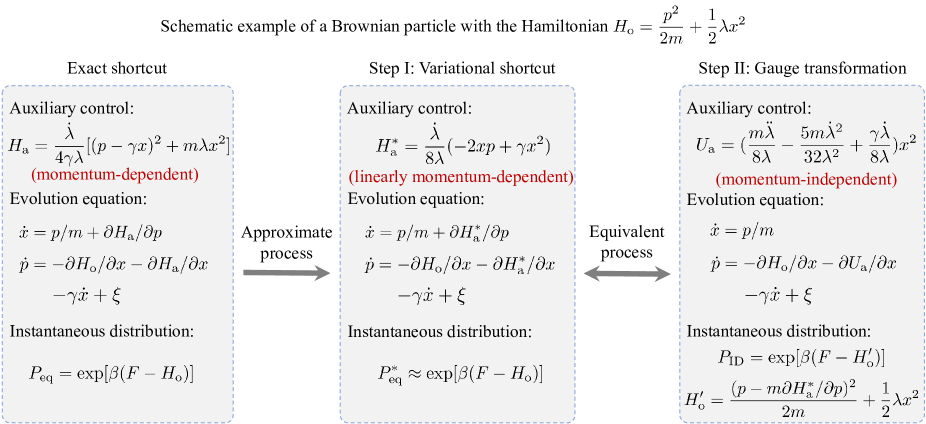
Figure 1: (Color online) Schematic example of a Brownian particle with the Hamiltonian $H_{\mathrm{o}}=p^{2}/(2m)+\lambda x^{2}/2$. The dynamical evolution of the system is governed by the Langevin equation, where $\gamma$ is the dissipation coefficient. In the shortcut scheme, a momentum-dependent auxiliary control $H_{\mathrm{a}}$ is added to escort the system distribution in the instantaneous equilibrium distribution $P_{\mathrm{eq}}$. In step I, a variational shortcut scheme is used to obtain an approximate auxiliary control $H_{\mathrm{a}}^{*}$ which can keep the system in the approximate equilibrium distribution $P_{\mathrm{eq}}^{*}$. In step II, a gauge transformation scheme is used to obtain a momentum-independent auxiliary control $U_{\mathrm{a}}$ which can maintain the system distribution in $P_{\mathrm{ID}}$.

II Geometric approach and the auxiliary Hamiltonian

In this section, we briefly review our geodesic approach of the shortcut to isothermality and show the possible experimental difficulties to apply the obtained auxiliary Hamiltonian.

Consider a system with the Hamiltonian $H_{\mathrm{o}}(\vec{x},\vec{p},\vec{\lambda})=\sum_{i}p_{i}^{2}/(2m)+U_{\mathrm{o}}(\vec{x},\vec{\lambda})$ immersed in a thermal reservoir with a constant temperature $T$. Here $\vec{x}\equiv(x_{1},x_{2},\cdots,x_{N})$ are coordinates, $\vec{p}\equiv(p_{1},p_{2},\cdots,p_{N})$ are momentum, $m$ is mass, and $\vec{\lambda}(t)\equiv(\lambda_{1},\lambda_{2},\cdots,\lambda_{M})$ are time-dependent control parameters. In the shortcut scheme, an auxiliary Hamiltonian $H_{\mathrm{a}}(\vec{x},\vec{p},t)$ is added to steer the evolution of the system along the instantaneous equilibrium states $P_{\mathrm{eq}}=\exp[\beta(F-H_{\mathrm{o}})]$ in the finite-time interval $t\in[0,\tau]$ with the boundary conditions $H_{\mathrm{a}}(0)=H_{\mathrm{a}}(\tau)=0.$ Here $F\equiv-\beta^{-1}\ln[\iint d\vec{x}d\vec{p}\exp(-\beta H_{\mathrm{o}})]$ is the free energy and $\beta=1/(k_{\mathrm{B}}T)$ is the inverse temperature with the Boltzmann constant $k_{\mathrm{B}}$. The probability distribution of the system’s microstate $P(\vec{x},\vec{p},t)$ evolves according to the Kramers equation

$$\frac{\partial P}{\partial t}=\sum_{i}[-\frac{\partial}{\partial x_{i}}(\frac{\partial H}{\partial p_{i}}P)+\frac{\partial}{\partial p_{i}}(\frac{\partial H}{\partial x_{i}}P+\gamma\frac{\partial H}{\partial p_{i}}P)+\frac{\gamma}{\beta}\frac{\partial^{2}P}{\partial p_{i}^{2}}],$$ (1)

where $H\equiv H_{\mathrm{o}}+H_{\mathrm{a}}$ is the total Hamiltonian, and $\gamma$ is the dissipation coefficient. The auxiliary Hamiltonian is proved to have the form $H_{\mathrm{a}}(\vec{x},\vec{p},t)=\dot{\vec{\lambda}}\cdot\vec{f}(\vec{x},\vec{p},\vec{\lambda})$ with $\vec{f}(\vec{x},\vec{p},\vec{\lambda})$ depending on

$$\sum_{i}[\frac{\gamma}{\beta}\frac{\partial^{2}H_{\mathrm{a}}}{\partial p_{i}^{2}}-\gamma p_{i}\frac{\partial H_{\mathrm{a}}}{\partial p_{i}}+\frac{\partial H_{\mathrm{a}}}{\partial p_{i}}\frac{\partial H_{\mathrm{o}}}{\partial x_{i}}-p_{i}\frac{\partial H_{\mathrm{a}}}{\partial x_{i}}]=\frac{dF}{dt}-\frac{\partial H_{\mathrm{o}}}{\partial t}.$$ (2)

The boundary conditions for the auxiliary Hamiltonian $H_{\mathrm{a}}(t)$ are presented explicitly as $\dot{\vec{\lambda}}(0)=\dot{\vec{\lambda}}(\tau)=0.$ The irreversible energy cost $W_{\mathrm{irr}}\equiv W-\Delta F$ in the shortcut scheme follows as (Li et al., 2022)

$$W_{\mathrm{irr}}=\sum_{\mu\nu}\int_{0}^{\tau}dt\dot{\lambda}_{\mu}\dot{\lambda}_{\nu}g_{\mu\nu},$$ (3)

where the positive semi-definite metric is $g_{\mu\nu}=\gamma\sum_{i}\langle(\partial f_{\mu}/\partial p_{i})(\partial f_{\nu}/\partial p_{i})\rangle_{\mathrm{eq}}$ with $\langle\cdot\rangle_{\mathrm{eq}}=\iint d\vec{x}d\vec{p}[\cdot]P_{\mathrm{eq}}.$ Here $W\equiv\langle\int_{0}^{\tau}dt\partial_{t}H\rangle$ is the mean work with $\langle\cdot\rangle$ representing the ensemble average over stochastic trajectories and $\Delta F\equiv F(\vec{\lambda}(\tau))-F(\vec{\lambda}(0))$ is the free energy difference. The metric $g_{\mu\nu}$ endows a Riemannian manifold in the space of thermodynamic equilibrium states marked by the control parameters $\vec{\lambda}.$ Minimizing the irreversible work in Eq.  (3) is equivalent to finding the geodesic path in the geometric space with the metric $g_{\mu\nu}$. This property allows us to obtain the optimal control protocol in the shortcut scheme by using methods developed in geometry (Berger, 2007).

Generally, the auxiliary Hamiltonian $H_{\mathrm{a}}$ are momentum-dependent that are hard to be implemented. For example, the auxiliary Hamiltonian for a one-dimensional harmonic system $H_{\mathrm{o}}=p^{2}/(2m)+\lambda x^{2}/2$ is obtained as (Li et al., 2017, 2022) $H_{\mathrm{a}}=\dot{\lambda}[(p-\gamma x)^{2}+m\lambda x^{2}]/(4\gamma\lambda).$ The quadratic momentum-dependent term $p^{2}$ and the linear momentum-dependent term $xp$ in the auxiliary Hamiltonian are hard to be realized in experiment due to the requirement of constantly monitoring the momentum (Guéry-Odelin et al., 2022).

III Approximate shortcut scheme

The variational shortcut scheme is an approximation of the exact shortcut scheme. The auxiliary Hamiltonian $H_{\mathrm{a}}$ in the exact shortcut scheme is replaced by the approximate auxiliary Hamiltonian $H_{\mathrm{a}}^{*}$. We define a semi-positive functional as (Li and Tu, 2021)

$$\mathcal{G}(H_{\mathrm{a}}^{*}) = \int d\vec{x}d\vec{p}[\sum_{i}(\frac{\gamma}{\beta}\frac{\partial^{2}H_{\mathrm{a}}^{*}}{\partial p_{i}^{2}}-\gamma p_{i}\frac{\partial H_{\mathrm{a}}^{*}}{\partial p_{i}}+\frac{\partial H_{\mathrm{o}}}{\partial x_{i}}\frac{\partial H_{\mathrm{a}}^{*}}{\partial p_{i}}$$ (4)

$$-p_{i}\frac{\partial H_{\mathrm{a}}^{*}}{\partial x_{i}})+\frac{\partial H_{\mathrm{o}}}{\partial t}-\frac{\mathrm{d}F}{\mathrm{d}t}]^{2}\mathrm{e}^{-\beta H_{\mathrm{o}}}\geqslant 0.$$

Finding the exact auxiliary Hamiltonian $H_{\mathrm{a}}^{*}=H_{\mathrm{a}}$ is equivalent to solving the variational equation (Li and Tu, 2021)

$$\frac{\delta\mathcal{G}(H_{\mathrm{a}}^{*})}{\delta H_{\mathrm{a}}^{*}}=0.$$ (5)

Instead of finding the exact solution, we use the above variational equation in Eq.$\ (\ref{seq:gaussvar})$ to solve for the possible approximate Hamiltonian $H_{\mathrm{a}}^{*}$ by finding the minimum value of $\mathcal{G}(H_{\mathrm{a}}^{*})$ in Eq.  (4). With the current variational method, we are able to neglect the quadratic term $p^{2}$ and remove the linear term $p$. The procedure is divided into two steps to remove the $p^{2}$ term with approximation and $p$ terms with gauge transformation, illustrated in Fig.  1 with the example Hamiltonian. The details are presented as follows.

Step I: Approximate auxiliary control without the quadratic term $p^{2}$. The first task is to remove the quadratic term $p^{2}$, by assuming the form of the auxiliary Hamiltonian

$$H_{\mathrm{a}}^{*}=\sum_{\mu i}\dot{\lambda}_{\mu}B_{\mu}(\vec{\lambda})x_{i}p_{i}+\sum_{\mu i}\dot{\lambda}_{\mu}C_{\mu i}(\vec{\lambda})p_{i}+\sum_{\mu}\dot{\lambda}_{\mu}D_{\mu}(\vec{x},\vec{\lambda}),$$ (6)

where $\vec{B}(\vec{\lambda}),$ $C(\vec{\lambda}),$ and $\vec{D}(\vec{x},\vec{\lambda})$ are functions determined by the variational equation  (5). Such approximation is valid for the case where the kinetic energy is negligible in the total energy. We illustrate how such approximation works with an example in the Appendix  A.

With such approximation, a distribution $P_{\mathrm{eq}}^{*}$ is reached as an approximation of the instantaneous equilibrium distribution $P_{\mathrm{eq}}$ with the variational shortcut scheme under the total Hamiltonian $H^{*}=H_{\mathrm{o}}+H_{\mathrm{a}}^{*}$, i.e., $P_{\mathrm{eq}}^{*}\approx P_{\mathrm{eq}}$. The mean work in the variational shortcut scheme follows as

$$W = \langle\int_{0}^{\tau}dt\frac{\partial H_{\mathrm{o}}}{\partial t}\rangle_{\mathrm{eq}}^{*}+\langle\int_{0}^{\tau}dt\frac{\partial H_{\mathrm{a}}^{*}}{\partial t}\rangle_{\mathrm{eq}}^{*}$$ (7)

$$\approx \Delta F^{*}+\gamma\sum_{i}\int_{0}^{\tau}dt\iint d\vec{x}d\vec{p}(\frac{\partial H_{\mathrm{a}}^{*}}{\partial p_{i}})^{2}P_{\mathrm{eq}}^{*},$$

where $\langle\cdot\rangle_{\mathrm{eq}}^{*}=\iint d\vec{x}d\vec{p}[\cdot]P_{\mathrm{eq}}^{*}.$ The free energy difference $\Delta F^{*}=\langle\int_{0}^{\tau}dt\partial_{t}H_{\mathrm{o}}\rangle_{\mathrm{eq}}^{*}$ is treated as an approximation to the free energy difference $\Delta F$ with high precision (Li and Tu, 2021). The additional energy cost of the variational shortcut scheme is evaluated by the irreversible work as

$$W_{\mathrm{irr}} \equiv W-\Delta F$$ (8)

$$\approx \gamma\sum_{\mu\nu i}\int_{0}^{\tau}dt\dot{\lambda}_{\mu}\dot{\lambda}_{\nu}\langle\frac{\partial f_{\mu}^{*}}{\partial p_{i}}\frac{\partial f_{\nu}^{*}}{\partial p_{i}}\rangle_{\mathrm{eq}}^{*},$$

where $H_{\mathrm{a}}^{*}=\dot{\vec{\lambda}}\cdot\vec{f}^{*}$ with $\vec{f}^{*}$ representing an approximation to the function $\vec{f}$ in Eq  (2). With a rescaling of the time $s=t/\tau,$ the irreversible work in Eq.  (8) is proved to follow the $1/\tau$ scaling which has been widely investigated in finite-time studies (Curzon and Ahlborn, 1975; Salamon and Berry, 1983; den Broeck, 2005; Schmiedl and Seifert, 2007b; Esposito et al., 2010; Wang and Tu, 2012; Ryabov and Holubec, 2016; Ma et al., 2018a, b, 2020; Tu, 2021). With the definition of a positive semi-definite metric

$$g_{\mu\nu}^{*}=\gamma\sum_{i}\langle\frac{\partial f_{\mu}^{*}}{\partial p_{i}}\frac{\partial f_{\nu}^{*}}{\partial p_{i}}\rangle_{\mathrm{eq}}^{*},$$ (9)

we can construct a Riemannian manifold on the space of the control parameters. The shortest curve connecting two equilibrium states is described through the thermodynamic length (Salamon and Berry, 1983; Crooks, 2007; Sivak and Crooks, 2012; Scandi and Perarnau-Llobet, 2019; Chen et al., 2021) $\mathcal{L}=\int_{0}^{\tau}dt\sqrt{\dot{\lambda}_{\mu}\dot{\lambda}_{\nu}g_{\mu\nu}^{*}}$ which gives a lower bound for the irreversible work $W_{\mathrm{irr}}$ as (Crooks, 2007)

$$W_{\mathrm{irr}} \geq \frac{\mathcal{L}^{2}}{\tau}.$$ (10)

Given boundary conditions $\vec{\lambda}(0)$ and $\vec{\lambda}(\tau),$ the lower bound in Eq.  (10) is reached by the optimal control scheme obtained by solving the geodesic equation

$$\ddot{\lambda}_{\mu}+\sum_{\nu\kappa}\Gamma_{\nu\kappa}^{\mu}\dot{\lambda}_{\nu}\dot{\lambda}_{\kappa} = 0,$$ (11)

where $\Gamma_{\nu\kappa}^{\mu}\equiv\sum_{\iota}(g^{*-1})_{\iota\mu}(\partial_{\lambda_{\kappa}}g_{\iota\nu}^{*}+\partial_{\lambda_{\nu}}g_{\iota\kappa}^{*}-\partial_{\lambda_{\iota}}g_{\nu\kappa}^{*})/2$ is the Christoffel symbol.

Step II: Equivalent process without the linear term $p$. The higher-order terms of the momentum in Eq.$\ (\ref{eq:apphamton})$ are removed for the experimental feasibility. In the variational shortcut scheme, the dynamical evolution of the system with the Hamiltonian $H=H_{\mathrm{o}}+H_{\mathrm{a}}^{*}$ is governed by the Langevin equation,

$$\dot{x}_{i}=\frac{p_{i}}{m}+\sum_{\mu}\dot{\lambda}_{\mu}B_{\mu}x_{i}+\sum_{\mu}\dot{\lambda}_{\mu}C_{\mu i},\\ \dot{p}_{i}=-\frac{\partial U_{\mathrm{o}}}{\partial x_{i}}-\sum_{\mu}\dot{\lambda}_{\mu}B_{\mu}p_{i}-\sum_{\mu}\dot{\lambda}_{\mu}\frac{\partial D_{\mu}}{\partial x_{i}}-\gamma\dot{x}_{i}+\xi_{i}(t),$$ (12)

where $\vec{\xi}\equiv(\xi_{1},\xi_{2},\cdots,\xi_{N})$ are the Gaussian white noise. During the evolution process described by Eq.  (12), the distribution of the system always stays in the instantaneous equilibrium distribution

$$P_{\mathrm{eq}}^{*}(\vec{x},\vec{p},\vec{\lambda})=\exp\{\beta[F(\vec{\lambda})-\sum_{i}p_{i}^{2}/(2m)-U_{\mathrm{o}}(\vec{x},\vec{\lambda})]\}.$$ (13)

With a gauge transformation (Sels and Polkovnikov, 2017; Li and Tu, 2021) $p_{i}\to p_{i}+m\sum_{\mu}\dot{\lambda}_{\mu}B_{\mu}x_{i}+m\sum_{\mu}\dot{\lambda}_{\mu}C_{\mu i},$ we can obtain an equivalent process controlled by the original Hamiltonian $H_{\mathrm{o}}$ and the auxiliary force $\vec{F}^{\mathrm{a}}$

$$\dot{x}_{i} = \frac{p_{i}}{m},$$

$$\dot{p}_{i} = -\frac{\partial U_{\mathrm{o}}}{\partial x_{i}}+F_{i}^{\mathrm{a}}-\gamma\dot{x}_{i}+\xi_{i}(t),$$ (14)

where the auxiliary force is explicitly presented as

$$F_{i}^{\mathrm{a}} = -\sum_{\mu}\dot{\lambda}_{\mu}\frac{\partial D_{\mu}}{\partial x_{i}}+m\sum_{\mu}\ddot{\lambda}_{\mu}B_{\mu}x_{i}+m\sum_{\mu\nu}\dot{\lambda}_{\mu}\dot{\lambda}_{\nu}\frac{\partial B_{\mu}}{\partial\lambda_{\nu}}x_{i}$$ (15)

$$+m\sum_{\mu\nu}\dot{\lambda}_{\mu}\dot{\lambda}_{\nu}B_{\mu}B_{\nu}x_{i}+m\sum_{\mu\nu}\dot{\lambda}_{\mu}\dot{\lambda}_{\nu}B_{\mu}C_{\nu i}$$

$$+m\sum_{\mu}\ddot{\lambda}_{\mu}C_{\mu i}+m\sum_{\mu\nu}\dot{\lambda}_{\mu}\dot{\lambda}_{\nu}\frac{\partial C_{\mu i}}{\partial\lambda_{\nu}}.$$

The distribution of the system in the process described by Eq.  (14) keeps in an instantaneous distribution with the fixed pattern

$$P_{\mathrm{ID}}(\vec{x},\vec{p},\vec{\lambda}) = \exp\{\beta[F(\vec{\lambda})-\sum_{i}(p_{i}-m\sum_{\mu}\dot{\lambda}_{\mu}B_{\mu}x_{i}$$ (16)

$$-m\sum_{\mu}\dot{\lambda}_{\mu}C_{\mu i})^{2}/(2m)-U_{\mathrm{o}}(\vec{x},\vec{\lambda})]\}.$$

As shown in Fig  2, with the boundary condition $\dot{\vec{\lambda}}(0)=\dot{\vec{\lambda}}(\tau)=0$, the instantaneous distribution $P_{\mathrm{ID}}(\vec{x},\vec{p},\vec{\lambda})$ in Eq.  (16) returns to the instantaneous equilibrium distribution $P_{\mathrm{eq}}^{*}(\vec{x},\vec{p},\vec{\lambda})$ in Eq.  (13) at $t=0$ and $\tau.$ It means that the system following the Langevin equation  (14) can evolve from an initial equilibrium state to another target equilibrium state. The operation of gauge transformation does not change the irreversible work in Eq.  (8). Therefore, the optimal control from the geodesic equation  (11) applies equally to the process described by the Langevin equation  (14). For the optimized protocol in the shortcut scheme, the boundary condition for $\dot{\vec{\lambda}}(t)$ is usually realized as discrete jumps at the beginning and end of the auxiliary force (Li et al., 2022). In the gauge transformation scheme, the system distribution in Eq.  (16) explicitly depends on $\dot{\vec{\lambda}}(t)$. And there is a mismatching between the initial equilibrium state $P_{\mathrm{eq}}^{*}(\vec{x},\vec{p},\vec{\lambda}(0))$ and the system distribution $P_{\mathrm{ID}}(\vec{x},\vec{p},\vec{\lambda}(0)),$ which can be offset for systems with weak inertial effect. We illustrate this claim in the following example.

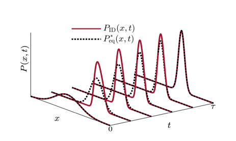
Figure 2: (Color online) Schematic of processes controlled by the variational shortcut scheme and the gauge transformation scheme. The system distribution of the variational shortcut scheme keeps in instantaneous equilibrium $P_{\mathrm{eq}}^{*}(x,t)$ during the evolution process while the instantaneous distribution of the gauge transformation scheme $P_{\mathrm{ID}}(x,t)$ deviates from the equilibrium distribution $P_{\mathrm{eq}}^{*}(x,t)$ for intermediate times $(0<t<\tau)$.

The steps to derive the experimentally testable protocol with minimum energy cost are shown in Fig.  1. In step I, we solve for the best possible auxiliary Hamiltonian $H_{\mathrm{a}}^{*}$ in Eq.  (5) by using the variational shortcut scheme. The geometric approach is then applied to minimize the irreversible work $W_{\mathrm{irr}}$ in Eq.  (8) and obtain the optimal protocol. In step II, the gauge transformation scheme with the operation in Eq.  (14) is carried out to obtain the final experimentally testable protocol with minimum energy cost.

IV Application

To demonstrate our strategy, we consider the Brownian motion in the harmonic potential with two controllable parameters $\vec{\lambda}=(\lambda_{1},\lambda_{2})$ with Hamiltonian as

$$H_{\mathrm{o}} = \frac{p^{2}}{2m}+\frac{\lambda_{1}}{2}x^{2}-\lambda_{2}x.$$ (17)

In the shortcut scheme (Li et al., 2017, 2022), the exact auxiliary Hamiltonian takes the form $H_{\mathrm{a}}(x,p,t)=\sum_{\mu=1}^{2}\dot{\lambda}_{\mu}f_{\mu}(x,p,\lambda_{1},\lambda_{2})$ where

$$f_{1} = \frac{(p-\gamma x)^{2}+m\lambda_{1}x^{2}}{4\gamma\lambda_{1}}-\frac{\lambda_{2}p}{2\lambda_{1}^{2}}+(\frac{\gamma\lambda_{2}}{2\lambda_{1}^{2}}-\frac{m\lambda_{2}}{2\gamma\lambda_{1}})x,$$

$$f_{2} = \frac{p}{\lambda_{1}}-\frac{\gamma x}{\lambda_{1}}.$$ (18)

With the application of the geometric approach proposed in Ref. (Li et al., 2022), the geodesic (optimal) protocol with minimum energy cost can be obtained as

$$\dot{\lambda}_{1} = \frac{w}{\tau}\sqrt{\frac{\lambda_{1}^{3}}{\lambda_{1}+\gamma^{2}/m}},$$

$$\frac{\lambda_{2}}{\lambda_{1}} = a\frac{t}{\tau}+b,$$ (19)

where $w=-\{2\sqrt{1+\gamma^{2}/(m\lambda_{1})}+\ln[\sqrt{1+\gamma^{2}/(m\lambda_{1})}-1]-\ln[\sqrt{1+\gamma^{2}/(m\lambda_{1})}+1]\}\mid_{\lambda_{1}(0)}^{\lambda_{1}(\tau)}$, $a=[\lambda_{2}(\tau)\lambda_{1}(0)-\lambda_{2}(0)\lambda_{1}(\tau)]/[\lambda_{1}(\tau)\lambda_{1}(0)]$, and $b=\lambda_{2}(0)/\lambda_{1}(0)$ are constants. Here $\vec{\lambda}(0)=(\lambda_{1}(0),\lambda_{2}(0))$ and $\vec{\lambda}(\tau)=(\lambda_{1}(\tau),\lambda_{2}(\tau))$ are boundary conditions. The momentum-dependent terms in Eq.  (18) hinder the implementation of the shortcut scheme in experiment.

We assume that the approximate auxiliary Hamiltonian takes the form

$$H_{\mathrm{a}}^{*}=a_{1}(t)px+a_{2}(t)p+a_{3}(t)x^{2}+a_{4}(t)x,$$ (20)

where $a_{1}(t),$ $a_{2}(t),$ $a_{3}(t),$ and $a_{4}(t)$ are coefficients to be determined. And the variational functional in Eq.  (4) follows as

$$\mathcal{G} = \iint dxdp\{[a_{1}p^{2}+(\gamma a_{1}+2a_{3})xp+(\gamma a_{2}+a_{4})p$$ (21)

$$-m(a_{1}x+a_{2})(\lambda_{1}x-\lambda_{2})]^{2}+\frac{2}{\beta}(a_{1}x+a_{2})(\dot{\lambda}_{1}x-\dot{\lambda}_{2})\}$$

$$\times\exp[-\beta(\frac{p^{2}}{2m}+\frac{\lambda_{1}}{2}x^{2}-\lambda_{2}x)].$$

The best possible auxiliary Hamiltonian $H_{\mathrm{a}}^{*}$ is obtained by minimizing the variational functional $\mathcal{G}$ over the parameters $a_{1}(t),$ $a_{2}(t),$ $a_{3}(t),$ and $a_{4}(t)$ as

$$H_{\mathrm{a}}^{*}=\dot{\lambda}_{1}(-\frac{px}{4\lambda_{1}}-\frac{3\lambda_{2}p}{4\lambda_{1}^{2}}+\frac{\gamma x^{2}}{8\lambda_{1}}+\frac{3\gamma\lambda_{2}x}{4\lambda_{1}^{2}})+\dot{\lambda}_{2}(\frac{p}{\lambda_{1}}-\frac{\gamma x}{\lambda_{1}})\text{.}$$ (22)

Detailed calculations are presented in Appendix  A.

We then apply the geometric approach to derive the optimal protocol with minimum energy cost. With the auxiliary Hamiltonian in Eq.  (22), the geometric metric in Eq.  (9) follows as

$$g = \left(\begin{array}[]{cc}\frac{\gamma}{16\beta\lambda_{1}^{3}}+\frac{\gamma\lambda_{2}^{2}}{\lambda_{1}^{4}}&-\frac{\gamma\lambda_{2}}{\lambda_{1}^{3}}\\ -\frac{\gamma\lambda_{2}}{\lambda_{1}^{3}}&\frac{\gamma}{\lambda_{1}^{2}}\end{array}\right).$$ (25)

The geodesic equation with the metric in Eq.  (25) takes the form

$$\ddot{\lambda}_{1}-\frac{3\dot{\lambda}_{1}^{2}}{2\lambda_{1}}=0,$$

$$\ddot{\lambda}_{2}-\frac{2\dot{\lambda}_{1}\dot{\lambda}_{2}}{\lambda_{1}}+\frac{\dot{\lambda}_{1}^{2}\lambda_{2}}{2\lambda_{1}^{2}}=0.$$ (26)

The solution for Eq.  (26) is analytically obtained as

$$\lambda_{1}(t) = \frac{1}{[(\lambda_{1}^{-\frac{1}{2}}(\tau)-\lambda_{1}^{-\frac{1}{2}}(0))\frac{t}{\tau}+\lambda_{1}^{-\frac{1}{2}}(0)]^{2}},$$

$$\lambda_{2}(t) = \frac{(\frac{\lambda_{2}(\tau)}{\lambda_{1}(\tau)}-\frac{\lambda_{2}(0)}{\lambda_{1}(0)})\frac{t}{\tau}+\frac{\lambda_{2}(0)}{\lambda_{1}(0)}}{[(\lambda_{1}^{-\frac{1}{2}}(\tau)-\lambda_{1}^{-\frac{1}{2}}(0))\frac{t}{\tau}+\lambda_{1}^{-\frac{1}{2}}(0)]^{2}}.$$ (27)

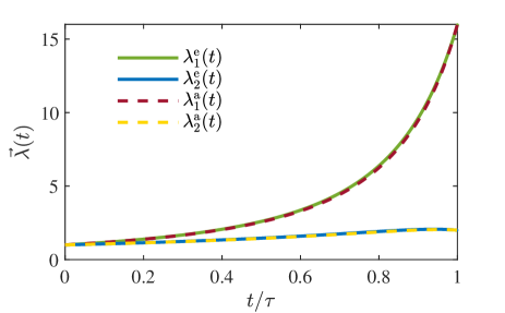
Figure 3: (Color online) Geodesic protocols for the exact shortcut scheme and the variational shortcut scheme. We have set the parameters as $m=0.01,$ $\gamma=1,$ and $k_{\mathrm{B}}T=1.$ The protocols change from $\vec{\lambda}(0)=(1,1)$ to $\vec{\lambda}(\tau)=(16,2).$ The solid lines are the geodesic protocol $\vec{\lambda}^{\mathrm{e}}(t)$ for the exact shortcut scheme in Eq.$\ (\ref{eq:geoprotocol})$ and the dashed lines are the geodesic protocol $\vec{\lambda}^{\mathrm{a}}(t)$ for the variational shortcut scheme in Eq.$\ (\ref{eq:anageodeseq})$. The geodesic protocol for the variational shortcut scheme (dashed lines) keeps close to the one for the exact shortcut scheme (solid lines).

In Fig.  3, we compare geodesic protocols for the exact shortcut scheme and the variational shortcut scheme. The parameters are chosen as $\vec{\lambda}(0)=(1,1),$ $\vec{\lambda}(\tau)=(16,2),$ $m=0.01,$ $\gamma=1,$ and $k_{\mathrm{B}}T=1.$ The geodesic protocol for the variational shortcut scheme $\vec{\lambda}^{\mathrm{a}}(t)$ (dashed lines) is in close proximity to the one for the exact shortcut scheme $\vec{\lambda}^{\mathrm{e}}(t)$ (solid lines), which supports our claim that the variational shortcut scheme can approximately reproduce the results of the exact shortcut scheme.

Note that there are still linear terms of the momentum in Eq.  (22). In the second step, we remove the remaining momentum-dependent terms by using the gauge transformation scheme. The Langevin equation for the variational shortcut scheme with the Hamiltonian $H=H_{\mathrm{o}}+H_{\mathrm{a}}^{*}$ follows as

$$\dot{x}=\frac{p}{m}-\frac{\dot{\lambda}_{1}x}{4\lambda_{1}}-\frac{3\dot{\lambda}_{1}\lambda_{2}}{4\lambda_{1}^{2}}+\frac{\dot{\lambda}_{2}}{\lambda_{1}},\\ \dot{p}=-\lambda_{1}x+\lambda_{2}+\frac{\dot{\lambda}_{1}p}{4\lambda_{1}}-\frac{\gamma\dot{\lambda}_{1}x}{4\lambda_{1}}-\frac{3\gamma\dot{\lambda}_{1}\lambda_{2}}{4\lambda_{1}^{2}}+\frac{\gamma\dot{\lambda}_{2}}{\lambda_{1}}-\gamma\dot{x}+\xi(t).$$ (28)

With the gauge transformation

$$p\to p-\frac{m\dot{\lambda}_{1}x}{4\lambda_{1}}-\frac{3m\dot{\lambda}_{1}\lambda_{2}}{4\lambda_{1}^{2}}+\frac{m\dot{\lambda}_{2}}{\lambda_{1}},$$ (29)

the Langevin equation  (28) is transformed into

$$\dot{x} = p,$$

$$\dot{p} = -\lambda_{1}x+\lambda_{2}+F_{\mathrm{a}}-\gamma p+\xi(t),$$ (30)

where the auxiliary force follows as

$$F_{\mathrm{a}} \equiv (\frac{5m\dot{\lambda}_{1}^{2}}{16\lambda_{1}^{2}}-\frac{\gamma\dot{\lambda}_{1}}{4\lambda_{1}}-\frac{m\ddot{\lambda}_{1}}{4\lambda_{1}})x-\frac{3\gamma\dot{\lambda}_{1}\lambda_{2}}{4\lambda_{1}^{2}}+\frac{\gamma\dot{\lambda}_{2}}{\lambda_{1}}$$ (31)

$$+\frac{27m\dot{\lambda}_{1}^{2}\lambda_{2}}{16\lambda_{1}^{3}}-\frac{2m\dot{\lambda}_{1}\dot{\lambda}_{2}}{\lambda_{1}^{2}}-\frac{3m\ddot{\lambda}_{1}\lambda_{2}}{4\lambda_{1}^{2}}+\frac{m\ddot{\lambda}_{2}}{\lambda_{1}}.$$

In the dynamics governed by the transformed Langevin equation  (30), there is no momentum-dependent term in the driving force. The auxiliary potential corresponding to the driving force in Eq.  (31) is obtained as

$$U_{\mathrm{a}} = \frac{m\ddot{\lambda}_{1}}{8\lambda_{1}}x^{2}+\frac{\gamma\dot{\lambda}_{1}}{8\lambda_{1}}x^{2}-\frac{5m\dot{\lambda}_{1}^{2}}{32\lambda_{1}^{2}}x^{2}-\frac{m\ddot{\lambda}_{2}}{\lambda_{1}}x-\frac{27m\dot{\lambda}_{1}^{2}\lambda_{2}}{16\lambda_{1}^{3}}x$$ (32)

$$+\frac{2m\dot{\lambda}_{1}\dot{\lambda}_{2}}{\lambda_{1}^{2}}x+\frac{3m\ddot{\lambda}_{1}\lambda_{2}}{4\lambda_{1}^{2}}x-\frac{\gamma\dot{\lambda}_{2}}{\lambda_{1}}x+\frac{3\gamma\dot{\lambda}_{1}\lambda_{2}}{4\lambda_{1}^{2}}x.$$

The system can be approximately transformed from an initial equilibrium state to another one within finite time. During intermediate driving process, the system follows the instantaneous distribution

$$P_{\mathrm{ID}}(x,p,\vec{\lambda}) = \exp\{\beta[F(\vec{\lambda})-\frac{1}{2m}(p+\frac{m\dot{\lambda}_{1}}{4\lambda_{1}}x$$ (33)

$$+\frac{3m\dot{\lambda}_{1}\lambda_{2}}{4\lambda_{1}^{2}}-\frac{m\dot{\lambda}_{2}}{\lambda_{1}})^{2}-U_{\mathrm{o}}(x,\vec{\lambda})]\},$$

which is an approximation to the instantaneous equilibrium states $P_{\mathrm{eq}}$.

To validate the variational shortcut scheme and the gauge transformation scheme, we compare the distributions $P_{\mathrm{eq}}^{*}(x,p,\vec{\lambda})$ and $P_{\mathrm{ID}}(x,p,\vec{\lambda})$ with that of the exact shortcut scheme $P_{\mathrm{eq}}(x,p,\vec{\lambda})$. The variational shortcut scheme and the gauge transformation scheme are respectively implemented through the Hamiltonian $H_{\mathrm{o}}+H_{\mathrm{a}}^{*}$ and $H_{\mathrm{o}}+U_{\mathrm{a}}$ while the exact shortcut scheme is realized through the Hamiltonian $H_{\mathrm{o}}+H_{\mathrm{a}}$. The distance between the instantaneous equilibrium distribution $P_{\mathrm{eq}}$ and the distribution in the variational shortcut scheme $P=P_{\mathrm{eq}}^{*}$ or the distribution in the gauge transformation scheme $P=P_{\mathrm{ID}}$ are evaluated through the Jensen-Shannon divergence (Lin, 1991; Endres and Schindelin, 2003; Majtey et al., 2005; Feng and Crooks, 2008)

$$\mathrm{D}(P||P_{\mathrm{eq}})=\frac{1}{2}\int d\vec{x}d\vec{p}(P\ln\frac{2P}{P+P_{\mathrm{eq}}}+P_{\mathrm{eq}}\ln\frac{2P_{\mathrm{eq}}}{P+P_{\mathrm{eq}}}).$$ (34)

We plot the Jensen-Shannon divergence $\mathrm{D}(P||P_{\mathrm{eq}})$ as a function of evolution time $t$ in Fig.  4. The protocol $\vec{\lambda}^{\mathrm{e}}(t)$ in Eq.  (19) is used to realize different driving schemes. Red triangles, green circles, and blue squares respectively represent the distance from the equilibrium distribution to the distribution of the gauge transformation scheme $(H_{\mathrm{o}}+U_{\mathrm{a}})$, the variational shortcut scheme $(H_{\mathrm{o}}+H_{\mathrm{a}}^{*})$, and the exact shortcut scheme $(H_{\mathrm{o}}+H_{\mathrm{a}})$. The distribution of the exact shortcut scheme closely follows the instantaneous equilibrium distribution while the distribution of the variational shortcut scheme initially drives the system away from equilibrium and then gradually back to the final equilibrium state. Compared with the variational shortcut scheme, the distribution of the gauge transformation scheme further departs from the instantaneous equilibrium distribution but still returns to the target equilibrium state approximately. These results therefore demonstrate that the gauge transformation scheme can reconcile the experimental feasibility and the target of transforming the system to the final equilibrium state with high precision.

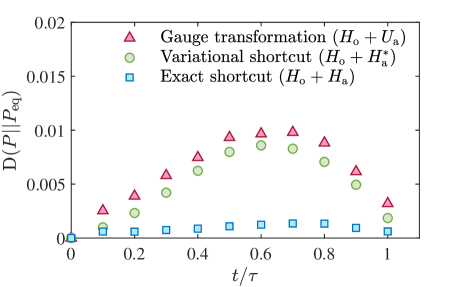
Figure 4: (Color online) Distance $\mathrm{D}(P||P_{\mathrm{eq}})$ between the instantaneous equilibrium distribution $P_{\mathrm{eq}}$ and the distribution in the variational shortcut scheme $P=P_{\mathrm{eq}}^{*}$ or the distribution in the gauge transformation scheme $P=P_{\mathrm{ID}}$. The gauge transformation scheme (red triangles), the variational shortcut scheme (green circles), and the exact shortcut scheme (blue squares) are implemented through the Hamiltonian $H_{\mathrm{o}}+U_{\mathrm{a}},$ $H_{\mathrm{o}}+H_{\mathrm{a}}^{*},$ and $H_{\mathrm{o}}+H_{\mathrm{a}},$ respectively. The distance is evaluated by using the Jensen-Shannon divergence (Lin, 1991; Endres and Schindelin, 2003; Majtey et al., 2005; Feng and Crooks, 2008). The protocol $\vec{\lambda}^{\mathrm{e}}(t)$ in Eq.  (19) is chosen to realize different schemes for fair comparison.

We also compare the irreversible work $W_{\mathrm{irr}}=W-\Delta F$ for different driving schemes. In the gauge transformation scheme, the variational shortcut scheme, and the exact shortcut scheme, the total Hamiltonian $H$ takes the form as $H_{\mathrm{o}}+U_{\mathrm{a}},$ $H_{\mathrm{o}}+H_{\mathrm{a}}^{*},$ and $H_{\mathrm{o}}+H_{\mathrm{a}},$ respectively. The exact shortcut scheme is carried out through the geodesic protocol $\vec{\lambda}^{\mathrm{e}}(t)$ in Eq.  (19) while the variational shortcut scheme and the gauge transformation scheme are carried out through the geodesic protocol $\vec{\lambda}^{\mathrm{a}}(t)$ in Eq.  (27). Fig.  5 shows the irreversible work of the gauge transformation scheme (red triangles), the variational shortcut scheme (green circles), and the exact shortcut scheme (blue squares) for different durations $\tau.$ The mean work is an average over $10^{5}$ stochastic trajectories. The irreversible work of the gauge transformation scheme coincides well with that of the variational shortcut scheme for different driving durations $\tau$, which demonstrates that the gauge transformation scheme can also well reproduce the energetic cost of the variational shortcut scheme. The irreversible work of the exact shortcut scheme is smaller than that of the gauge transformation scheme in short driving processes and gradually coincides with later as the duration increases. This shows that the energy cost of the gauge transformation scheme can keep pace with that of the exact shortcut scheme while approximately transform the system to the target equilibrium state with high precision.

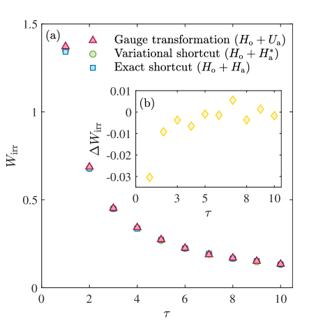
Figure 5: (Color online) The irreversible work for the gauge transformation scheme (red triangles), the variational shortcut scheme (green circles), and the exact shortcut scheme (blue squares) with different durations $\tau$. The mean work are obtained from $10^{5}$ stochastic trajectories. The irreversible work of the gauge transformation scheme and the variational shortcut scheme coincide well, which demonstrates that the gauge transformation scheme works. The protocol $\vec{\lambda}^{\mathrm{e}}(t)$ in Eq.  (19) is used to perform the exact shortcut scheme while the protocol $\vec{\lambda}^{\mathrm{a}}(t)$ in Eq.  (27) is used to realize the variational shortcut scheme and the gauge transformation scheme. The inset shows the difference of the irreversible work $\Delta W_{\mathrm{irr}}$ between the exact shortcut scheme and the gauge transformation scheme for different durations $\tau$.

V Conclusion and discussion

In conclusion, we have presented a momentum-independent driving scheme to approximately transform the system from an initial equilibrium state to another target equilibrium state. The momentum-dependent terms in the auxiliary Hamiltonian have been removed through the variational method and the gauge transformation. A geometric approach has been applied to minimize the energy cost of the driving scheme. The optimal protocol with minimum energy cost is obtained by solving the geodesic equation with methods developed in Riemannian geometry. We have tested our driving strategy by using a Brownian particle system with two controllable parameters. The simulation results prove that our scheme can achieve the task of rapidly driving the system to the target equilibrium state with high precision while reconcile the experimental feasibility. Our scheme should offer an experimentally testable control protocol with minimum energy cost for approximately realizing the shortcut scheme.

The gauge transformation scheme and the variational shortcut scheme are approximate shortcut schemes. The remaining distance between the final distribution of the approximate shortcut scheme and the target equilibrium distribution can be replenished through a short relaxation. Such a deviation is caused by the absence of the high-order momentum-dependent terms in the variational shortcut scheme. The momentum-dependent terms will play an important role in the dynamical evolution if the inertial effect is significantly obvious. Therefore, the deviation could be reduced if the inertial effect is weaken. The operation of changing variables to remove momentum-dependent terms in the gauge transformation scheme is similar to the fast-forward scheme in the field of shortcuts to adiabaticity (Masuda and Nakamura, 2009; Torrontegui et al., 2012; Martínez-Garaot et al., 2016; Jarzynski et al., 2017; Patra and Jarzynski, 2017; Sels and Polkovnikov, 2017; Kolodrubetz et al., 2017; Guéry-Odelin et al., 2019, 2022). Our operation is implemented for systems following the stochastic dynamics.

In the underdamped case, the controlled Brownian motion has been investigated in different experimental platforms (Li et al., 2010; Cunuder et al., 2016; Ciliberto, 2017; Hoang et al., 2018; Dago et al., 2021). The driving force of our approximate shortcut scheme in Eq.  (32) only depends on the position of the system. It is promising to test our approximate shortcut scheme in experiment.

VI Acknowledgement

Acknowledgement.–This work is supported by the National Natural Science Foundation of China (NSFC) (Grants No. 12088101, No. 11875049, No. U1930402, and No. U1930403) and the National Basic Research Program of China (Grant No. 2016YFA0301201).

Appendix A Illustration of how the approximation of the variational shortcut scheme works

We illustrate how the approximation of the variational shortcut scheme works with an example of a Brownian particle moving in the harmonic potential with the Hamiltonian $H_{\mathrm{o}}=p^{2}/(2m)+\lambda(t)x^{2}/2,$ where $\lambda(t)$ is the control parameter. In the shortcut scheme, the auxiliary Hamiltonian follows as (Li et al., 2017)

$$H_{\mathrm{a}}=\frac{\dot{\lambda}}{4\gamma\lambda}[(p-\gamma x)^{2}+m\lambda x^{2}].$$ (35)

To evaluate the contribution of each momentum-dependent term to the shortcut scheme, we introduce the characteristic length $l_{\mathrm{c}}\equiv(k_{\mathrm{B}}T/\lambda(0))^{1/2}$, the characteristic time $\tau_{1}=m/\gamma$ and $\tau_{2}=\gamma/\lambda(0)$ to rescale the Hamiltonian. The dimensionless coordinate, momentum, time, and control protocol are defined as $\tilde{x}\equiv x/l_{\mathrm{c}},$ $\tilde{p}\equiv p\tau_{2}/(ml_{\mathrm{c}})$, $s\equiv t/\tau_{2},$ and $\tilde{\lambda}\equiv\lambda/\lambda(0)$. The dimensionless Hamiltonian are then obtained as

$$\tilde{H}_{\mathrm{o}}\equiv\frac{H_{\mathrm{o}}}{k_{\mathrm{B}}T}=\alpha\frac{\tilde{p}^{2}}{2}+\frac{1}{2}\tilde{\lambda}\tilde{x}^{2},$$ (36)

and

$$\tilde{H}_{\mathrm{a}} \equiv \frac{H_{\mathrm{a}}}{k_{\mathrm{B}}T}=\frac{\tilde{\lambda}^{\prime}}{4\tilde{\lambda}}[\alpha^{2}(\tilde{p}-\frac{\tilde{x}}{\alpha})^{2}+\alpha\tilde{\lambda}\tilde{x}^{2}]$$ (37)

$$= \alpha^{2}\frac{\tilde{\lambda}^{\prime}\tilde{p}^{2}}{4\tilde{\lambda}}-\alpha\frac{\tilde{\lambda}^{\prime}\tilde{x}\tilde{p}}{2\tilde{\lambda}}+\alpha\frac{\tilde{\lambda}^{\prime}\tilde{x}^{2}}{4}+\frac{\tilde{\lambda}^{\prime}\tilde{x}^{2}}{4\tilde{\lambda}},$$

where $\tilde{\lambda}^{\prime}\equiv d\tilde{\lambda}/ds$ and $\alpha\equiv m\lambda(0)/\gamma^{2}.$ Note that there are different orders of $\alpha$ in the above expressions of $\tilde{H}_{\mathrm{o}}$ and $\tilde{H}_{\mathrm{a}}.$ If we assume that $\alpha\ll 1$, the second-order term of $\alpha$ in Eq.  (37), i.e., the $\tilde{p}^{2}$ term in $\tilde{H}_{\mathrm{a}}$ can be neglected, which means that the approximation of the variational shortcut scheme is valid. The dimensionless parameter $\alpha$ is small if the mass $m$ or the stiffness coefficient $\lambda(0)$ is small compared to the dissipation coefficient $\gamma.$

Appendix B The approximate auxiliary Hamiltonian

We start from the functional in Eq.  (21). With the minimization of parameters $a_{1}(t),$ $a_{2}(t),$ $a_{3}(t),$ and $a_{4}(t)$, we obtain a set of equations:

$$3a_{1}+\gamma\beta[(\gamma a_{1}+2a_{3})\bar{x^{2}}+(\gamma a_{2}+a_{4})\bar{x}]+\lambda_{1}\beta(a_{1}\bar{x^{2}}+a_{2}\bar{x})+\dot{\lambda}_{1}\beta\bar{x^{2}}-\dot{\lambda}_{2}\beta\bar{x}=0,$$

$$\gamma a_{2}+a_{4}+(\gamma a_{1}+2a_{3})\bar{x}+\lambda_{1}(a_{1}\bar{x}+a_{2})+\dot{\lambda}_{1}\bar{x}-\dot{\lambda}_{2}=0,$$

$$(\gamma a_{1}+2a_{3})\bar{x^{2}}+(\gamma a_{2}+a_{4})\bar{x}=0,$$

$$(\gamma a_{1}+2a_{3})\bar{x}+\gamma a_{2}+a_{4}=0,$$ (38)

where $\bar{x^{n}}\equiv\int_{-\infty}^{\infty}x^{n}\exp[-\beta(\lambda_{1}x^{2}/2-\lambda_{2}x)]dx/\int_{-\infty}^{\infty}\exp[-\beta(\lambda_{1}x^{2}/2-\lambda_{2}x)]dx$ with $n=1,2,\cdots.$ We can analytically obtain that $\bar{x}=\lambda_{2}/\lambda_{1},$ $\bar{x^{2}}=1/(\beta\lambda_{1})+\lambda_{2}^{2}/\lambda_{1}^{2},$ $\bar{x^{3}}=3\lambda_{2}/(\beta\lambda_{1}^{2})+\lambda_{2}^{3}/\lambda_{1}^{3},$ and $\bar{x^{4}}=3/(\beta^{2}\lambda_{1}^{2})+6\lambda_{2}^{2}/(\beta\lambda_{1}^{3})+\lambda_{2}^{4}/\lambda_{1}^{4}.$ The integral over $p$ has been calculated in Eq.  (38). The solution of Eq.  (38) is obtained as

$$a_{1}(t) = -\frac{\dot{\lambda}_{1}}{4\lambda_{1}},$$

$$a_{2}(t) = \frac{\dot{\lambda}_{2}}{\lambda_{1}}-\frac{3\dot{\lambda}_{1}\lambda_{2}}{4\lambda_{1}^{2}},$$

$$a_{3}(t) = \frac{\gamma\dot{\lambda}_{1}}{8\lambda_{1}},$$

$$a_{4}(t) = \frac{3\gamma\dot{\lambda}_{1}\lambda_{2}}{4\lambda_{1}^{2}}-\frac{\gamma\dot{\lambda}_{2}}{\lambda_{1}}.$$ (39)

Then we derive the approximate auxiliary Hamiltonian in Eq.  (22) according to Eq.  (20).

Appendix C The stochastic simulation

The dynamical evolution of the Brownian particle system is described by the Langevin equation

$$\dot{x} = \frac{\partial H}{\partial p},$$

$$\dot{p} = -\frac{\partial H}{\partial x}-\gamma\frac{\partial H}{\partial p}+\xi(t),$$ (40)

where $H$ is the total Hamiltonian and $\xi(t)$ is the standard Gaussian white noise satisfying $\langle\xi(t)\rangle=0$ and $\langle\xi(t)\xi(t^{\prime})\rangle=2\gamma k_{\mathrm{B}}T\delta(t-t^{\prime})$. We introduce the characteristic length $l_{\mathrm{c}}\equiv(k_{\mathrm{B}}T/\lambda_{1}(0))^{1/2}$, the characteristic time $\tau_{1}=m/\gamma$ and $\tau_{2}=\gamma/\lambda_{1}(0)$. Then the dimensionless coordinate, momentum, time, and control protocol can be defined as $\tilde{x}\equiv x/l_{\mathrm{c}},$ $\tilde{p}\equiv p\tau_{2}/(ml_{\mathrm{c}})$, $s\equiv t/\tau_{2},$ $\tilde{\lambda}_{1}\equiv\lambda_{1}/\lambda_{1}(0),$ and $\tilde{\lambda}_{2}\equiv\lambda_{2}/(\lambda_{1}(0)l_{\mathrm{c}}).$ The dimensionless Langevin equation follows as

$$\tilde{x}^{\prime} = \frac{1}{\alpha}\frac{\partial\tilde{H}}{\partial\tilde{p}},$$

$$\tilde{p}^{\prime} = -\frac{1}{\alpha}\frac{\partial\tilde{H}}{\partial\tilde{x}}-\frac{1}{\alpha^{2}}\frac{\partial\tilde{H}}{\partial\tilde{p}}+\sqrt{2}\zeta(s)/\alpha\text{,}$$ (41)

where $\tilde{\tau}\equiv\tau/\tau_{2}$ and $\alpha\equiv\tau_{1}/\tau_{2}$. The prime represents the derivative with respective to the dimensionless time $s$. $\zeta(s)$ is a Gaussian white noise satisfying $\langle\zeta(s)\rangle=0$ and $\langle\zeta(s_{1})\zeta(s_{2})\rangle=\delta(s_{1}-s_{2})$. The Euler algorithm is used to solve the Langevin equation as

$$\tilde{x}(s+\delta s) = \tilde{x}(s)+\frac{1}{\alpha}\frac{\partial\tilde{H}}{\partial\tilde{p}}\delta s,$$

$$\tilde{p}(s+\delta s) = \tilde{p}(s)-\frac{1}{\alpha}\frac{\partial\tilde{H}}{\partial\tilde{x}}\delta s-\frac{1}{\alpha^{2}}\frac{\partial\tilde{H}}{\partial\tilde{p}}\delta s+\sqrt{2\delta s}\theta(s)/\alpha\text{,}$$ (42)

where $\delta s$ is the time step and $\theta(s)$ is a random number following the Gaussian distribution with zero mean and unit variance. The work of the stochastic trajectories follows as

$$\tilde{w}\equiv\frac{w}{k_{B}T} = \int_{0}^{1}\frac{\partial\tilde{H}}{\partial s}ds\approx\sum\frac{\partial\tilde{H}}{\partial s}\delta s.$$ (43)

In simulation, we set the boundary conditions as $\vec{\lambda}(0)=(1,1)$ and $\vec{\lambda}(\tau)=(16,2).$ The parameters are chosen as $k_{\mathrm{B}}T=1$, $\gamma=1$, and $m=0.01$. The mean work is the ensemble average over the work of $10^{5}$ stochastic trajectories.