A generalized expansion method for computing Laplace–Beltrami eigenfunctions on manifolds

Abstract.

Eigendecomposition of the Laplace–Beltrami operator is instrumental for a variety of applications from physics to data science. We develop a numerical method of computation of the eigenvalues and eigenfunctions of the Laplace–Beltrami operator on a smooth bounded domain based on the relaxation to the Schrödinger operator with finite potential on a Riemannian manifold and projection in a special basis. We prove spectral exactness of the method and provide examples of calculated results and applications, particularly, in quantum billiards on manifolds.

1. Introduction

The Laplace–Beltrami operator plays an important role in the differential equations that describe many physical systems. These include, for example, vibrating membranes, fluid flow, heat flow, and solutions to the Schrödinger equation. Another example is that of spectral partitions—collections of $k$ pairwise disjoint open subsets such that the sum of their first Laplace–Beltrami eigenvalues is minimal [13, 14, 38, 39]. This has a wide class of applications including data classification [32], interacting agents [18, 16, 19], and so on. In all the above applications, the fundamental question is how to efficiently compute the eigenvalues of the Laplace–Beltrami operator in an arbitrary domain with a proper boundary condition. Also, the Laplace–Beltrami operator is crucial to understanding systems described by nonlinear Schrödinger equations, such as the propagation of Langmuir waves in an ionized plasma [24, 7], the single-particle ground-state wavefunction in a Bose–Einstein condensate [7], the slowly-varying envelope of light waves in Kerr media [20], and water surface wave packets [41].

The Laplace–Beltrami operator of a scalar function $f$ on a Riemannian manifold $(\mathcal{M},g)$ is defined as the surface divergence of the vector field gradient of $f$,

(1.1) $$\Delta_{g}f=\nabla\cdot\nabla f.$$

The divergence of a vector field $X$ with metric $g$ is (in Einstein notation)

(1.2) $$\nabla\cdot X=\frac{1}{\sqrt{|g|}}\partial_{i}\mathopen{}\mathclose{{}\left(\sqrt{|g|}X^{i}}\right),$$

and the gradient of a scalar function $f$ is

(1.3) $$(\operatorname{grad}f)^{i}=\partial^{i}f=g^{ij}\partial_{j}f.$$

From above, we obtain the Laplace–Beltrami operator acting on functions over $(\mathcal{M},g)$,

(1.4) $$\Delta_{g}f=\frac{1}{\sqrt{|g|}}\partial_{i}\mathopen{}\mathclose{{}\left(\sqrt{|g|}g^{ij}\partial_{j}f}\right).$$

In general, the Helmholtz equation (i.e. Laplace–Beltrami eigenvalue problem) with Dirichlet boundary conditions on $\Omega\subset(\mathcal{M},g)$ is

(1.5) $$\begin{cases}-\Delta_{g}u(x)=\lambda u(x),&x\in\Omega\\ u(x)=0,&x\in\partial\Omega.\end{cases}$$

In this paper, we develop a numerical method to find the eigenvalues and eigenfunctions of the Laplace–Beltrami operator with Dirichlet and periodic boundary conditions for arbitrary domains on various surfaces. The idea is highly motivated by the Schrödinger operator and is based off the method given in [27]. By using the Schrödinger operator relaxation, we relax the eigenvalue problem on an arbitrary domain into the eigenvalue problem for a Schrödinger operator on a regular domain which is convenient for the numerical discretization.

In [34], comparable methods on manifolds using linear and cubic FEM operators and discrete geometric Laplacians are explored, and [17] provides a method for hyperbolic domains. There is extensive literature on the Laplacian for planar regions [26, 29, 12, 8, 1]. In methods for solving nonlinear Schrödinger equations, finite difference discretizations of the Laplace operator are often used [5, 6, 16]. It is likely many of these methods above can be extended to the Laplace–Beltrami operator on manifolds. The method we present in this paper has some immediate advantages over the finite difference method—since the boundary of domains are characterized by a potential function (see Theorem 7), no creation of a complicated mesh is needed, allowing for more generic domains and producing smooth solutions. Also, the method has promise to be quite robust in discretizing the operator on domains with corners (as in Table I), especially in applications when computation of many eigenvalues is required, whereas the finite difference method is notoriously inefficient on such domains.

The rest of the paper is organized as follows. In Section 2, we recall the Schrödinger operator and introduce the generalized expansion method. We discuss and prove the convergence and accuracy of the relaxation and approximation in Section 3 and show extensive numerical experiments in Section 4. We investigate applications to spherical domains, periodic domains, and billiard problems in Section 5 and draw some conclusion in Section 6.

2. Generalized Expansion Method

The time-independent Schrödinger equation on a Riemannian manifold $\mathcal{M}$ with metric $g$, potential ${V}(x)$, and energy levels $E_{n}$ is

(2.1) $$\hat{H}\psi_{n}(x)=\mathopen{}\mathclose{{}\left[-\Delta_{g}+{V}(x)}\right]\psi_{n}(x)=E_{n}\psi_{n}(x),\\$$

where $\Delta_{g}$ is the Laplace–Beltrami operator on $(\mathcal{M},g)$ as in (1.4). The Schrödinger equation is an eigenvalue problem for the Schrödinger operator $\hat{H}=-\Delta_{g}+V(x)$. When

(2.2) $${V}(x)=\mathopen{}\mathclose{{}\left\{\begin{array}[]{ll}0&x\in\Omega\\ \infty&x\not\in\Omega,\end{array}}\right.$$

the eigenvalue problem for $\hat{H}$ is equivalent to (1.5). Eigenfunctions are normalized by setting

(2.3) $$\int_{\Omega}|\psi_{n}(x)|^{2}dx=1,$$

where $|\psi_{n}(x)|^{2}dx$ is a probability density.

In [27], a method is given to solve (1.5) with $g=I_{2}$ on any bounded smooth $\Omega\subset\mathbb{R}^{2}$ by embedding it in a rectangle, as in Figure 1. In order to evaluate the Laplace–Beltrami eigenvalues for $\Omega$ on a 2-D surface, we generalize this method when considering $\Omega$ as a smooth subset of a bounded manifold $S=(\mathcal{M},g)$ using a complete set of orthonormal eigenfunctions $\mathcal{F}^{S}_{\infty}=\{\phi_{n}\}_{n=1}^{\infty}$ on $S$ with corresponding eigenvalues $\{\lambda_{n}(S)\}_{n=1}^{\infty}$ (with $\lambda_{1}<\lambda_{2}\leq\lambda_{3}\leq\dots$). Here, we assume all $\phi_{n}\in\mathcal{F}^{S}_{\infty}$ have Dirichlet boundary conditions on $\partial S$, but for cases when $|\partial\Omega\cap\partial S|>0$, one may choose to use other boundary conditions to obtain solutions of (1.5) with $\mathopen{}\mathclose{{}\left.u}\right|_{x\in\partial\Omega\cap\partial S}\not\equiv 0$, as in the periodic examples in Section 5.2.

Figure 1. With the expansion method, a bounded domain $\Omega$ is embedded onto a rectangle $S$ with euclidean geometry and $\hat{H}$ is projected onto $\mathcal{F}^{S}_{N}$.

In this method, we use $\mathcal{F}^{S}_{N}=\{\phi_{n}\}_{n=1}^{N}$ as a basis on which we expand the operator $\hat{H}$ and seek solutions of (1.5), or the equivalent equation involving the eigenvalue problem of the Schrödinger operator $\hat{H}$,

(2.4) $$\hat{H}\psi(x)=\mathopen{}\mathclose{{}\left[-\Delta_{g}+\tilde{V}(x)}\right]\psi(x)=\lambda\psi(x),$$

with $\tilde{V}(x)$ defined as

(2.5) $$\tilde{V}(x)=\mathopen{}\mathclose{{}\left\{\begin{array}[]{ll}0&x\in\Omega\\ \infty&x\in S\setminus\Omega.\end{array}}\right.$$

We approximate $\tilde{V}(x)$ as

(2.6) $$V(x)=V_{0}\chi_{S\setminus\Omega}(x)=\mathopen{}\mathclose{{}\left\{\begin{array}[]{ll}0&x\in\Omega\\ V_{0}\gg 1&x\in S\setminus\Omega.\end{array}}\right.$$

This allows us to discretize the operator $\hat{H}\approx H_{N}$,

(2.7) $$H_{N_{nm}}=\langle\phi_{n},\hat{H}\phi_{m}\rangle=\lambda_{n}^{S}\delta_{nm}+\int_{S}V(x)\phi^{*}_{n}\phi_{m}dx,$$

where we truncate $n,m\leq N$. The eigenvalues and eigenvectors of $H_{N}$ approximate those of $\hat{H}$.

3. Convergence analysis

In this section, we provide a rigorous proof on the convergence of the proposed method in the sense of $V_{0}\rightarrow\infty$ and $N\rightarrow\infty$. To keep self-consistency of the paper, we first recall some definitions and preliminary results from [25, 36, 22].

Definition 1.

Suppose $A_{n}$ and $A$ are self-adjoint operators. We say that $A_{n}$ converges to $A$ in the strong resolvent sense, if

(3.1) $$\|(R_{A_{n}}(z)-R_{A}(z))\phi\|\to 0,\quad\forall\phi\in\mathfrak{D}(A_{n})$$

for some $z\in\Gamma=\mathbb{C}\setminus\Sigma,\Sigma=\sigma(A)\cup\bigcup_{n}\sigma\mathopen{}\mathclose{{}\left(A_{n}}\right)$ where the function $R_{A}(z)$ is the resolvent of $A$.

Definition 2.

A subset $\mathfrak{D}_{0}\subseteq\mathfrak{D}(A)$ is a core of $A$ when $\{(x,Ax):x\in\mathfrak{D}_{0}\}$ is dense in $\{(x,Ax):x\in\mathfrak{D}(A)\}$.

Lemma 3.

(6.36 of [36]): Let $A_{n},A$ be self-adjoint operators. Then $A_{n}$ converges to $A$ in the strong resolvent sense if there is a core $\mathfrak{D}_{0}$ of $A$ such that for any $\psi\in\mathfrak{D}_{0}$ we have $P_{n}\psi\in\mathfrak{D}\mathopen{}\mathclose{{}\left(A_{n}}\right)$ for $n$ sufficiently large and $A_{n}P_{n}\psi\rightarrow A\psi$.

Theorem 4.

(6.38 of [36]). Let $A_{n}$ and $A$ be self-adjoint operators. If $A_{n}$ converges to $A$ in the strong resolvent sense, we have $\sigma(A)\subseteq\lim_{n\rightarrow\infty}\sigma\mathopen{}\mathclose{{}\left(A_{n}}\right)$.

Theorem 5.

(2.2.3 of [25]). Let $L_{n}$ be a sequence of uniformly elliptic operators defined on an open set $D$ by

(3.2) $$L_{n}u:=-\sum_{i,j=1}^{N}\frac{\partial}{\partial x_{i}}\mathopen{}\mathclose{{}\left(a_{ij}^{n}(x)\frac{\partial u}{\partial x_{j}}}\right)+a_{0}^{n}(x)u.$$

We assume that, for fixed $i,j$, the sequence $a_{i,j}^{n}$ is bounded in $L^{\infty}$ and converge almost everywhere to a function $a_{i,j}$; we also assume that the sequence $a_{0}^{n}$ is bounded in $L^{\infty}$ and converges weakly-* in $L^{\infty}$ to a function $a_{0}$. Let $L$ be the (elliptic) operator defined on $D$ as in (3.2) by the functions $a_{i,j}$ and $a_{0}$. Then each eigenvalue of $L_{n}$ converges to the corresponding eigenvalue of $L$.

Theorem 6.

(9.29 of [22]) Let $u\in W^{2,p}(S)\cap C^{0}(\bar{S})$ satisfy $Lu=f$ in $S,u=\varphi$ on $\partial S$ where $f\in L^{p}(S),\varphi\in C^{\beta}(\bar{S})$ for some $\beta>0$, and suppose that $\partial S$ satisfies a uniform exterior cone condition. Then $u\in C^{\alpha}(\bar{S})$ for some $\alpha>0$.

Now, we prove spectral exactness of the expansion method in $V_{0}$ and $N$ in Theorems 7 and 9. We give an example of calculating solutions and the rate of convergence in $V_{0}$ of eigenvalues for the relaxed problem on an interval in Example 8. We provide intuition for efficient implementation of the expansion method in Remark 10.

Theorem 7.

The eigenvalues of the Schrödinger operator

(3.3) $$\hat{H}(V_{0})=-\Delta_{g}+V(x),\qquad V(x)=\mathopen{}\mathclose{{}\left\{\begin{array}[]{ll}0,&x\in\Omega\\ V_{0},&x\not\in\Omega\end{array}}\right.$$

acting on a bounded Riemannan manifold $(\mathcal{M},g)$, with $\Omega$ smooth in $(\mathcal{M},g)$ converge monotonically to the eigenvalues of $-\Delta_{g}$ with Dirichlet boundary conditions on $\Omega$ as $V_{0}\rightarrow\infty$.

Proof.

By considering the volume form on the manifold, we have the inner product:

(3.4) $$\langle f_{1},f_{2}\rangle_{g}=\int_{\mathcal{M}}\overline{f_{1}(x)}f_{2}(x)(\operatorname{det}g)^{1/2}dx_{1}\cdots dx_{n}$$

Now, from the Rayleigh quotient of an elliptic linear operator $\mathcal{L}$ on a Riemannian manifold $(\mathcal{M},g)$,

(3.5) $$R(\mathcal{L},u)=\frac{\langle u,\mathcal{L}u\rangle_{g}}{\langle u,u\rangle_{g}},$$

we have

(3.6) $$R(\hat{H}(V_{0}),u)=\frac{\langle u,-\Delta_{g}u\rangle_{g}}{\langle u,u\rangle_{g}}+\frac{\langle u,Vu\rangle_{g}}{\langle u,u\rangle_{g}}.$$

By the Courant-Fischer formula,

(3.7) $$\lambda_{k}(\hat{H}(V_{0}))=\inf_{\mathcal{Q}\in\mathcal{Q}_{k}}\sup_{u\in\mathcal{Q}}\mathopen{}\mathclose{{}\left(R(\hat{H},u)}\right)$$

with $\mathcal{Q}_{k}$ being the family of subspaces of $H_{0}^{1}(\mathcal{M})$ of dimension $k$, we obtain the following inequality,

(3.8) $$\lambda_{k}(\hat{H}(V_{0}^{*}))\geq\lambda_{k}(\hat{H}(V_{0})),\quad\text{for }V_{0}^{*}>V_{0},$$

giving us monotonicity. We also have for $u\in H^{1}_{0}(\mathcal{M})$ and as $V_{0}\rightarrow\infty$, $R(\hat{H}(V_{0}),u)<\infty$ if and only if $\operatorname{supp}(u)\subseteq\Omega$ almost everywhere. Hence, we have

(3.9) $$\lim_{V_{0}\rightarrow\infty}\lambda_{k}(\hat{H}(V_{0}))=\inf_{\mathcal{Q}^{*}\in\mathcal{Q}^{*}_{k}}\sup_{u\in\mathcal{Q}^{*}}\mathopen{}\mathclose{{}\left(R(\hat{H},u)}\right)$$

with $\mathcal{Q}^{*}_{k}$ being the family of subspaces of $H_{0}^{1}(\Omega)$ of dimension $k$. This is precisely the Courant-Fischer definition of the eigenvalues of the Laplace–Beltrami operator with Dirichlet boundary conditions on $\Omega$. ∎

Example 8.

Consider the regions $S=(0,2)$ and $\Omega=(0,1)$. The eigenvalues of the Helmholtz equation on $\Omega$,

(3.10) $$-v_{k}^{\prime\prime}=\mu_{k}v_{k},\qquad v_{k}(0)=v_{k}(1)=0,$$

can be approximated by the eigenvalues of the Schrödinger operator $\hat{H}_{V_{0}}=-\partial_{x}^{2}+V(x;V_{0})$ on $S$ with $V(x;V_{0})=V_{0}\chi_{S\setminus\Omega}(x)$ and large $V_{0}\gg 1$, with

(3.11) $$\hat{H}_{V_{0}}u_{k}=\lambda_{k}(V_{0})u_{k},\qquad u(0)=u(2)=0,$$

and rate of convergence

(3.12) $$|\lambda_{k}(V_{0})-\mu_{k}|\sim\frac{1}{\sqrt{V_{0}}}$$

up to a constant, as $V_{0}\uparrow\infty.$

Proof.

We have (3.10) has eigenvalues $\mu_{k}=\pi^{2}k^{2}$ for $k\in\mathbb{N}\setminus\{0\}$. Solutions to (3.11) are of the form:

(3.13) $$u_{k}=\begin{cases}\sin\sqrt{\lambda_{k}}x,&x\in(0,1]\\ \frac{\sin\sqrt{\lambda_{k}}}{\sinh\sqrt{V_{0}-\lambda_{k}}}\sinh(\sqrt{V_{0}-\lambda_{k}}(2-x)),&x\in(1,2).\end{cases}$$

By setting $u_{k}\in C^{1}(0,2)$, we arrive at

(3.14) $$\sqrt{\lambda_{k}}\cot\sqrt{\lambda_{k}}=-\sqrt{V_{0}-\lambda_{k}}\coth\sqrt{V_{0}-\lambda_{k}}\implies\frac{\sqrt{\lambda_{k}}}{\sin\sqrt{\lambda}_{k}}\sim\sqrt{V_{0}},$$

as $V_{0}\uparrow\infty$. We then have by Taylor expansion of $\sin(\cdot)$ about $\sqrt{\mu_{k}}$,

(3.15) $$\sin\sqrt{\lambda_{k}}=\sin(\sqrt{\lambda_{k}}-\sqrt{\mu_{k}}+\sqrt{\mu_{k}})\approx\pm(\sqrt{\lambda_{k}}-\sqrt{\mu_{k}})\sim\frac{\sqrt{\lambda_{k}}}{\sqrt{V_{0}}}\sim\frac{1}{\sqrt{V_{0}}}$$

since $\sin\sqrt{\mu_{k}}=0$. The last relation above arises from $\sqrt{\lambda_{k}}\sim\sqrt{\mu_{k}}$, a constant. Hence altogether,

(3.16) $$|\lambda_{k}-\mu_{k}|=|\sqrt{\lambda_{k}}-\sqrt{\mu_{k}}|\cdot|\sqrt{\lambda_{k}}+\sqrt{\mu_{k}}|\sim\frac{1}{\sqrt{V_{0}}}.$$

∎

Theorem 9.

Given a complete orthonormal basis $\mathcal{F}^{S}_{\infty}\subset H^{1}_{0}(S)$ of Laplace–Beltrami eigenfunctions on a bounded smooth domain $S=(\mathcal{M},g)$, the Dirichlet eigenvalues of the $N$-dimensional operator $H_{N}$ where $H_{N_{ij}}=\langle\phi_{i},\hat{H}\phi_{j}\rangle$ for $i,j\leq N$ converge to those of $\hat{H}$ as $N\rightarrow\infty$ where

(3.17) $$\hat{H}=-\Delta_{g}+V(x),\qquad V(x)\in L^{\infty}(S,\mathbb{R}).$$

The results in this theorem hold for Neumann and periodic boundary conditions as well, using the appropriate basis and Sobolev space.

Proof.

We first note

(3.18) $$H_{N}:\mathcal{F}^{S}_{N}\to\mathcal{F}^{S}_{N}\qquad\hat{H}:H^{1}_{0}(S)\to L^{2}(S),$$

where $\mathcal{F}^{S}_{N}=\operatorname{span}\{\phi_{j}\}_{j=1}^{N}$. We also have, by the definition of $H_{N}$, with $u=\sum_{j=1}^{\infty}c_{j}\phi_{j}$:

(3.19) $$H_{N}u :=\sum_{i=1}^{N}\mathopen{}\mathclose{{}\left(\sum_{k=1}^{N}\langle\phi_{i},\hat{H}\phi_{k}\rangle c_{k}}\right)\phi_{i}=\sum_{j=1}^{N}\langle\phi_{j},\hat{H}u\rangle\phi_{j}=P_{N}\hat{H}u$$

$$P_{N}v :=\sum_{j=1}^{N}\langle\phi_{j},v\rangle\phi_{j}$$

Furthermore, by convention we may extend the domain of $H_{N}$ to $H^{1}_{0}(S)$ by the following extension, which we will now use in the proof:

(3.20) $$H_{N}u:=P_{N}\hat{H}P_{N}u.$$

Without loss of generality, because $V(x)$ is bounded we can assume further that $V(x)\in[0,\infty)$ since the resulting spectra are merely shifted by a constant $\alpha$ when adding $\alpha$ to $V(x)$, hence we have $\operatorname{ker}(\hat{H}^{*})=\emptyset$ by injectivity and self-adjointness, giving us $\overline{\operatorname{ran}(\hat{H})}=L^{2}(S)$. We consider the set $\mathfrak{D}_{0}=\mathcal{F}^{S}_{\infty}\cap H^{1}_{0}(S)$, and we have $\overline{\mathfrak{D}_{0}}=L^{2}(S)=\overline{H^{1}_{0}(S)}$, and $\overline{H\mathfrak{D}_{0}}=\overline{\operatorname{span}\{H\phi_{j}\}_{j=1}^{\infty}}\cap\overline{L^{2}(S)}=L^{2}(S)$, by $V\in L^{\infty}(S)$. Hence, the graph $\{(x,\hat{H}x):x\in\mathfrak{D}_{0}\}$ is dense in $\{(x,\hat{H}x):x\in\mathfrak{D}(\hat{H})\}$, therefore $\mathfrak{D}_{0}$ is a core of $\hat{H}$. Furthermore, we have for all $\psi\in\mathfrak{D}_{0}$ that $P_{N}\psi\in\operatorname{span}\{\phi_{j}\}_{j=1}^{N}$ and $H_{N}\psi=P_{N}\hat{H}P_{N}\psi\to\hat{H}P_{N}\psi$, so by Lemma 3 we have strong convergence in the resolvent sense, and hence the conditions for Theorem 4 are met, and we have

(3.21) $$\lim_{N\to\infty}\sigma(H_{N})\supseteq\sigma(\hat{H}).$$

Now, it is well-known these operators have purely point spectra. We consider $V_{N}=P_{N}V$ and consider $\lambda_{N}\to\lambda_{*}$, some converging sequence of eigenvalues of $H_{N}$ with corresponding eigenvectors $u_{N}$. We have $P_{N}u_{N}=u_{N}$ and $P_{N}\Delta_{g}u_{N}=\Delta_{g}u_{N}$, giving us

$$H_{N}u_{N}=(-\Delta_{g}+V_{N})u_{N}=\lambda_{N}u_{N} \implies\lambda_{N}\in\sigma(-\Delta_{g}+V_{N}),$$

$$\sigma(-\Delta_{g}+V_{N})\longrightarrow\sigma(\hat{H}) \implies\lambda_{*}\in\sigma(\hat{H})$$

by Theorem 5, giving us

(3.22) $$\lim_{N\to\infty}\sigma(H_{N})\subseteq\sigma(\hat{H}).$$

Altogether, we have the desired result,

(3.23) $$\lim_{N\to\infty}\sigma(H_{N})=\sigma(\hat{H}).$$

Similar proofs can be made for the Neumann and periodic boundary cases. ∎

Remark 10.

For fixed $\Omega,\ V_{0},$ and $N$, an efficient implementation of this method is to seek an integrable domain $S\supset\Omega$ to minimize the following value involving the $L^{2}$-induced norm of the difference of the operators acting on the finite-dimensional space $\mathcal{F}^{S}_{N}$:

(3.24) $$\tau_{\Omega}(S):=V_{0}^{-1}\cdot\mathopen{}\mathclose{{}\left\|\mathopen{}\mathclose{{}\left.[\hat{H}-H_{N}(S)]}\right|_{\mathcal{F}^{S}_{N}}}\right\|_{\mathcal{B}(L^{2}(\Omega),L^{2}(\Omega))}=V_{0}^{-1}\cdot\mathopen{}\mathclose{{}\left\|V-\sum_{j=1}^{N}\langle\phi_{j},V\rangle\phi_{j}}\right\|_{L^{\infty}(\Omega)}$$

This procedure is equivalent to fitting a domain $\Omega$ properly into a solvable set $S$ so that the potential $V$ that characterizes $\Omega$ is well-approximated by $P_{N}V$.

4. Numerical Accuracy

Note that contrary to Theorem 7, in practice, the method loses accuracy if $V_{0}$ is chosen to be too large, due to floating point round-off errors. We provide a numerical example here. One can identify the shape of a triangle given the spectrum of the solution to the Helmholtz equation [23], and a formula can be derived for the Laplacian eigenvalues $\lambda_{n}$ of an equilateral triangle with Dirichlet boundary conditions [11], for positive integers $p$ and $q$,

(4.1) $$\lambda_{n}\equiv\lambda_{pq}=\Big{(}\frac{4\pi}{3}\Big{)}^{2}(p^{2}+q^{2}-pq),\ 1\leq q\leq p/2,$$

where $\lambda_{n}$ is a multiple eigenvalue with multiplicity 2 if $p\neq 2q$. $\lambda_{n}$ is in units ${1}/{a^{2}}$ and $a$ is the side length of the triangle. In Figure 2, we compare these known eigenvalues with those computed using the expansion method with varying $V_{0}$. Although we showed monotonic convergence as $V_{0}\to\infty$ in 3, a properly chosen value would be at about $V_{0}\approx 2.6\times 10^{6}$, depending on how many eigenvalues one wishes to compute and the chosen domain.

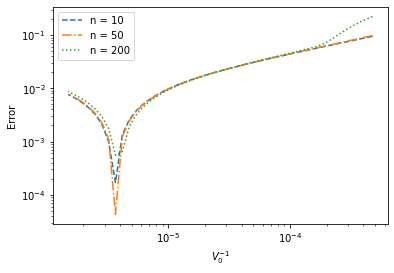
Figure 2. Average relative error for the first $n$ eigenvalues for varying values of $V_{0}^{-1}$.

We now solve for the L-shaped domain modes numerically using the expansion method. Here, we use $\mathcal{F}^{S}_{N}=\{\phi_{n}\}_{n=1}^{N}$ on $S=(0,2)^{2}$ and $\Omega=S\setminus[1,2)^{2}$ with

(4.2) $$\phi_{n}=\phi_{(n_{1},n_{2})}=\sqrt{\frac{2}{a_{1}}}\sin\mathopen{}\mathclose{{}\left(\frac{\pi}{a_{1}}n_{1}x_{1}}\right)\sqrt{\frac{2}{a_{2}}}\sin\mathopen{}\mathclose{{}\left(\frac{\pi}{a_{2}}n_{2}x_{2}}\right)=\sin\mathopen{}\mathclose{{}\left(\frac{\pi}{2}n_{1}x_{1}}\right)\sin\mathopen{}\mathclose{{}\left(\frac{\pi}{2}n_{2}x_{2}}\right),$$

just as in [27]. We provide examples of the computed eigenmodes in Figure 3. This L-shaped domain is common in the literature, as it is a simple construction of a domain with no closed form solution [37, 40, 21]. In Table I, we provide the computed eigenvalues corresponding to the provided eigenmodes, along with those computed using a second-order finite difference operator (see [30]), with uniform grid spacings $h$ for both the $x$ and $y$ axes:

$$H^{\operatorname{FD}} =-(I\otimes D^{2}_{x}+D_{y}^{2}\otimes I)+V_{\operatorname{d}}$$

$$D_{x}^{2} =D_{y}^{2}=\frac{1}{h^{2}}\mathopen{}\mathclose{{}\left(\begin{array}[]{cccc}-2&1&&\\ 1&\ddots&\ddots&\\ &\ddots&\ddots&1\\ &&1&-2\end{array}}\right)$$

$$V_{\operatorname{d}} =\mathopen{}\mathclose{{}\left(\begin{array}[]{cccccccc}v_{11}&&&&&&&\\ &v_{21}&&&&&&\\ &&\ddots&&&&&\\ &&&v_{N1}&&&&\\ &&&&v_{22}&&&\\ &&&&&\ddots&&\\ &&&&&&&v_{NN}\end{array}}\right)$$

$$v_{nm} =V(x_{n},y_{m}).$$

The results in Table I of the computation of Laplacian eigenvalues for the L-shaped domain using the expansion method and FD are compared with the known values from [37], which were remarkably computed with up to 8 digits of accuracy. This comparison provides numerical validation of the expansion method.

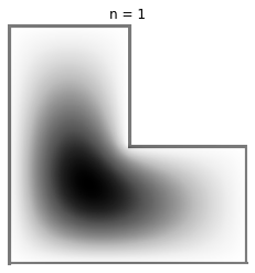
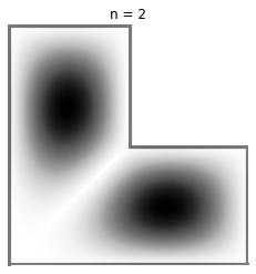
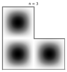
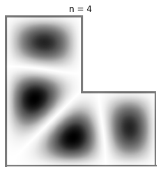
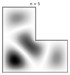
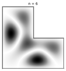
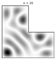
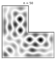
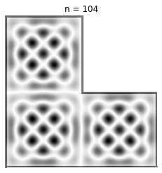
Figure 3. Various states $|\psi|$ for the L-shaped region on a plane, computed using the expansion method.

$n$	FD Method	Exp. Method	Known Values
1	9.33328	9.63359	9.63972
2	14.8927	15.1964	15.1973
3	19.4634	19.7385	19.7392
4	29.2480	29.5209	29.5215
5	31.2302	31.8982	31.9126
6	40.3540	41.4629	41.4745
20	98.9878	101.585	101.605
50	239.487	250.777	250.785
104	462.102	493.543	493.480

$n$	FD Method	Exp. Method	Known Values
1	9.69329	10.1213	9.63972
2	14.9296	15.7156	15.1973
3	19.4097	20.1868	19.7392
4	28.5903	29.8785	29.5215
5	31.171	32.8286	31.9126
6	39.4412	42.9975	41.4745
20	91.6147	105.747	101.605
50	179.955	255.717	250.785
104	306.101	514.121	493.480

Table I. Computed Laplacian eigenvalues of the L-shaped region. Both schemes used a discretized 2-D Schrödinger operator in $\mathbb{R}^{N\times N}$ and $V_{0}=2.1\times 10^{5}$. $N=2500$ (left) and $N=225$ (right). The known values were taken from [37].

5. Applications

5.1. Spherical domains.

The expansion method can be used on a variety of manifolds, and for example, on a spherical surface. The eigenfunctions of the Laplace–Beltrami operator on a sphere are the spherical harmonics $Y$, which are solutions to

(5.1) $$\frac{1}{\sqrt{|g|}}\partial_{i}\mathopen{}\mathclose{{}\left(\sqrt{|g|}g^{ij}\partial_{j}Y(\theta,\phi)}\right)=\lambda Y(\theta,\phi)$$

where

(5.2) $$g=\mathopen{}\mathclose{{}\left[\begin{array}[]{cc}1&0\\ 0&\sin^{2}\theta\end{array}}\right].$$

Spherical harmonics $Y_{m\ell}$ provide a set of orthonormal functions and thus can be used as a basis. These functions are defined over the indices $m$ (integers) and $\ell$ (non-negative integers), where $Y_{m\ell}$ is defined for $|m|\leq\ell$. These functions are known explicitly ($P^{m}_{\ell}$ denoting associated Legendre polynomials),

(5.3) $$Y_{m\ell}=\mathopen{}\mathclose{{}\left\{\begin{array}[]{ll}(-1)^{m}\sqrt{2}\sqrt{\frac{2\ell+1}{4\pi}\frac{(\ell-|m|)!}{(\ell+|m|)!}}P_{\ell}^{|m|}(\cos\theta)\sin(|m|\varphi)&\text{ if }m<0\\ \sqrt{\frac{2\ell+1}{4\pi}}P_{\ell}^{m}(\cos\theta)&\text{ if }m=0\\ (-1)^{m}\sqrt{2}\sqrt{\frac{2\ell+1}{4\pi}\frac{(\ell-m)!}{(\ell+m)!}}P_{\ell}^{m}(\cos\theta)\cos(m\varphi)&\text{ if }m>0.\end{array}}\right.$$

The eigenfunctions of the Laplace–Beltrami operator with Dirichlet boundary conditions for some smooth region on a sphere can be expressed in $L^{2}(S)$ as linear combinations of spherical harmonics,

(5.4) $$\psi_{j}(\phi,\theta)=\sum_{\begin{subarray}{c}m,\ \ell\end{subarray}}c^{(j)}_{m\ell}Y_{\ell}^{m}(\phi,\theta).$$

As in (2.7), the matrix representation of the Schrödinger operator $\hat{H}$ in the space composed of the basis functions is given by

(5.5) $$H_{ij}=\int_{S}Y_{i}(\phi,\theta)\hat{H}Y_{j}(\phi,\theta)ds,$$

where $i$ and $j$ each represent an index pair $(m,\ell)$. By substituting $\mathopen{}\mathclose{{}\left[-\Delta_{g}+V(\phi,\theta)}\right]$ for $\hat{H}$ and making a change of variables, we obtain $ds=r\sin(\theta)d\phi d\theta$ on the unit sphere and the discretized Hamiltonian,

(5.6) $$H_{N_{ij}} =\langle Y_{i},\hat{H}Y_{j}\rangle$$

$$=\ell(\ell+1)\delta_{ij}+V_{0}\int_{S}Y_{i}(\phi,\theta)Y_{j}(\phi,\theta)\sin{(\theta)}d\phi d\theta,$$

for a large value $V_{0}\gg 1$. We can then calculate the matrix $H_{N}$ and its eigenpairs numerically. We then expand the eigenvectors back into the spherical harmonic basis.

Using the presented method, we have calculated and plotted the first twelve states for the half-sphere, octant, and spherical square alongside their planar analogs (in grayscale) to illustrate the utility of the expansion method. We have plotted the absolute value to distinguish the nodal lines.

Figure 4. The first 12 modes of a half-sphere (above) compared to those of a planar disk (below). Notice the ordering of the degenerate modes does not match.

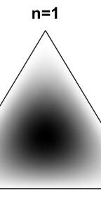
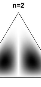
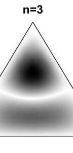
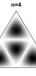
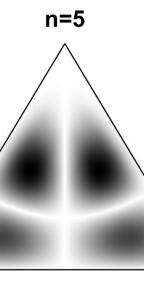
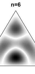
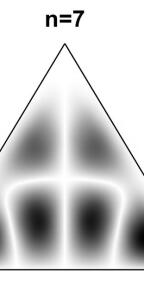
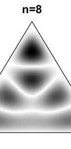
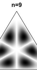
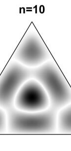
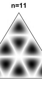
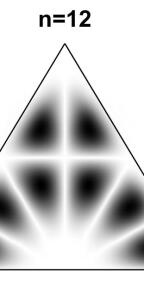
Figure 5. The first 12 modes of the spherical octant (above) compared with those of an equilateral triangle (below). Notice the ordering of the degenerate modes does not match.

Figure 6. The first 12 modes of the hexant or spherical square (above) and those of a planar square (below).

5.2. Periodic domains.

The Schrödinger equation (2.1) in periodic domains has important application to solving for Bloch states of electrons in a crystalline solid [28]. Here we present an extension of the expansion method to computing eigenvalues and eigenfunctions of the Schrodinger and Helmholtz equations for periodic domain.

Definition 11.

A $d$-dimensional lattice $\Gamma_{B}$ is the set $\{\sum x_{i}{b}_{i}:x_{i}\in\mathbb{Z}\}$ with vectors $\{{b}_{i}\}\in\mathbb{R}^{d}$. Consequently, $\Gamma_{B}=\mathbb{Z}^{d}B$ for $B\in GL(d,\mathbb{R})$, the group of $d\times d$ invertible real matrices.

Definition 12.

The dual of a lattice $\Gamma_{B}$ is $\Gamma_{B}^{*}=\{{x}\in\mathbb{R}^{d}:\langle{x},{y}\rangle\in\mathbb{Z},\forall{y}\in\Gamma_{B}\}$. Consequently, $\Gamma_{B}^{*}=\mathbb{Z}^{d}B^{-T}$ for $B\in GL(d,\mathbb{R})$.

Definition 13.

A $d$-dimensional flat torus $T_{B}$ is defined as the quotient space $T_{B}={\mathbb{R}^{d}}/{\Gamma_{B}}$ for $B\in GL(d,\mathbb{R})$.

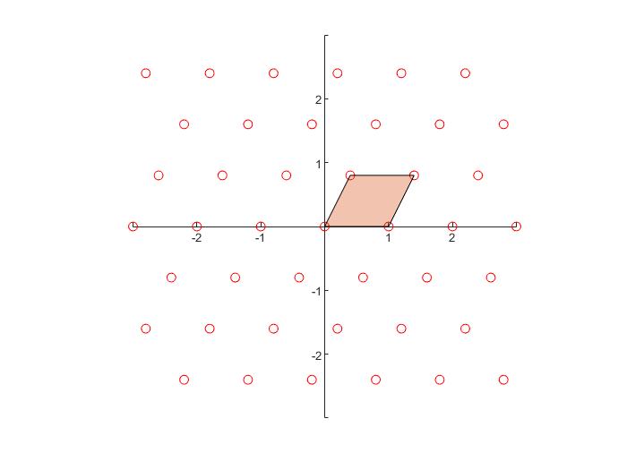
Figure 7. Fundamental region of a lattice in $\mathbb{R}^{2}$ (left). A $2$-dimensional flat torus is formed by periodic boundary conditions over opposite edges of the fundamental region (middle). An example of a periodic domain—the dark regions indicate holes with Dirichlet boundary conditions where $V_{0}\gg 1$ (right).

For Euclidean space $\mathbb{R}^{d}$, eigenfunctions for $-\Delta$ on $\Omega=T_{B}$ are of the form $\phi_{n}({x})=\exp(2\pi i\langle{x},{w}\rangle)$ for $w\in\Gamma^{*}_{B}$, and the eigenvalues are $-\Delta\phi_{n}({x})/\phi_{n}({x})=4\pi^{2}\|{w}\|^{2}$. We extend the expansion method to these domains using these eigenpairs and the potential $V(x)=V_{0}\chi_{\Omega^{c}}(x)$. This allows us to compute eigenfunctions of domains with mixed Dirichlet and periodic boundaries. In Figure 7, we show an example of a periodic domain with a hole removed in each cell.

Just as in previous sections, the expansion method for a flat torus is given by the discretization of $\hat{H}$ where

(5.7) $$\begin{array}[]{ll}H_{nm}&=\langle\phi_{n},\hat{H}\phi_{m}\rangle\\ &=\lambda_{n}(T_{B})\delta_{nm}+V_{0}{\int}_{T_{B}\setminus\Omega}\phi_{n}^{*}\phi_{m}dx\end{array}$$

and $\lambda_{n}(T_{B})$ denotes the eigenvalues of the flat torus $T_{B}$ itself. The eigenvalues and eigenvectors of $H_{nm}$ are approximations of the eigenvalues and eigenfunctions of $\hat{H}$ (in the basis $\{\phi_{n}\}$). Figure 8 displays computed eigenmodes on a periodic domain with holes (domain shown in Figure 13).

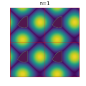
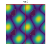
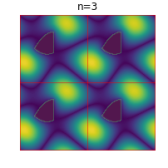
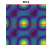
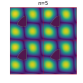
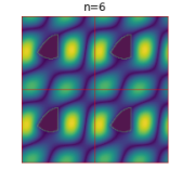
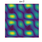
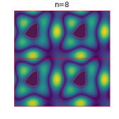
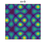
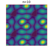
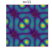
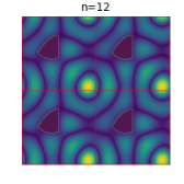
Figure 8. The absolute value of the first 12 computed eigenfunctions for a periodic domain (same domain shown in Figure 13). We impose periodic conditions on the boundary of the square cells and Dirichlet conditions along the boundary of the omitted shape.

5.3. Spectral Clustering and Billiard Trajectories

Here, we give several examples of implementing the generalized expansion method to heuristically explore quantum signatures of chaos in classical billiards from computed eigenvalue statistics. This is similar to what is done in [27, 2], but on manifolds. We use the following conjectures as foundations for the heuristic.

Conjecture 14.

(Berry-Tabor) The spectral value spacings of generic integrable systems coincide with those of uncorrelated random numbers from a Poisson process.

Conjecture 15.

(Bohigas-Gianonni-Schmit) The spectral value spacings of generic classically chaotic systems coincide with those of random matrices from the Gaussian Ensembles.

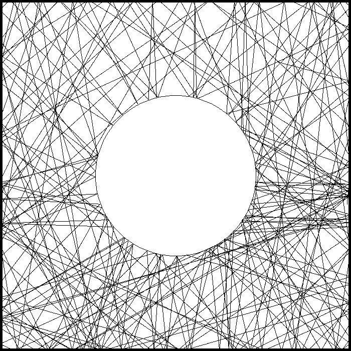
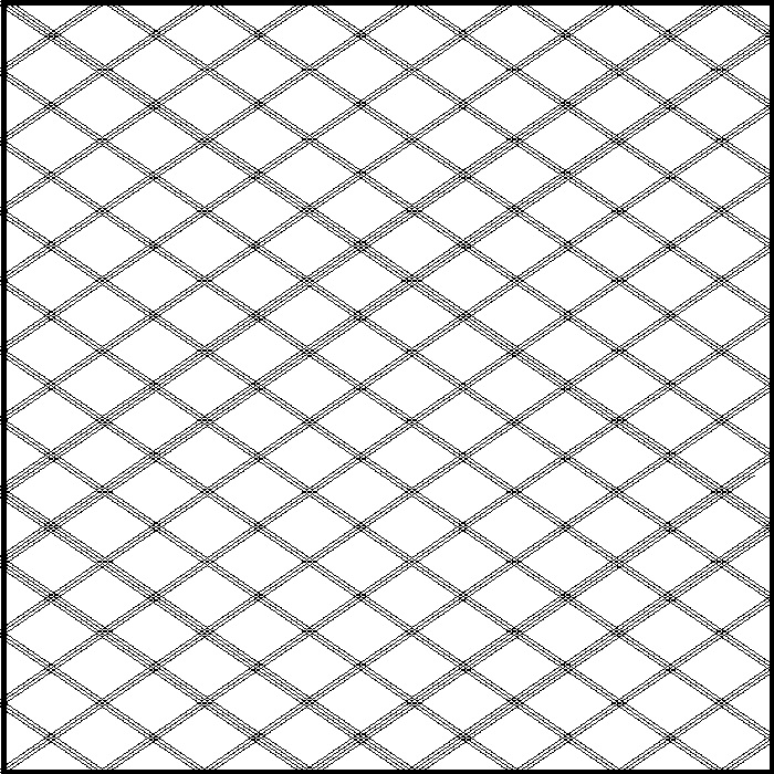
Figure 9. These billiards give simple examples of chaotic trajectories (left) and regular trajectories (right). The chaotic billiard here is the well-known Sinai Billiard.

It is understood that generic systems have zero probability to have symmetries, and Hamiltonians with symmetries have degenerate states that are not relevant to the discussion of billiard dynamics [10]. Hence, in this discussion and in common practice, we desymmetrize the domains as much as possible before computing eigenvalues in order to ignore the symmetric modes, and we are left with billiards which we assume are sufficiently generic. Further insight into these conjectures and their relation to random matrix theory can be found in [3, 35].

Now, by considering the normalized distribution of the computed first $n$ spacings between consecutive Laplace–Beltrami eigenvalues of some desymmetrized region $\Omega$ with Dirichlet boundary conditions, we apply the Conjectures 14 and 15 as a heuristic to verify the trajectory type (see Figure 9) of the following regions by comparing these distributions to the Poisson distribution $P_{0}(s)=e^{-s}$ and GOE distribution $P_{\operatorname{GOE}}(s)=\frac{1}{2}\pi se^{-\pi s^{2}/4}$.

Planar billiards.

As the Sinai Billiard is a well-known classically chaotic billiard, we have used this domain as an example to perform the generalized expansion method and compare the resulting eigenvalue spacing distribution to the expected GOE distribution. As the equilateral triangle is a known integrable system, we expect its eigenvalue spacing distribution to coincide with a Poisson distribution. Using the method, we indeed arrive at these results and show them in Figure 11. We perform, when possible, a terminating sequence of desymmetrizations on the domains, as shown in 10.

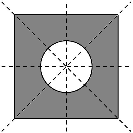
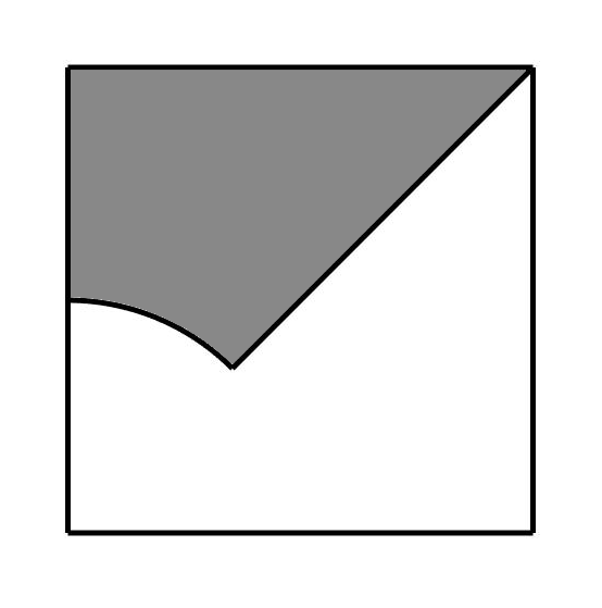
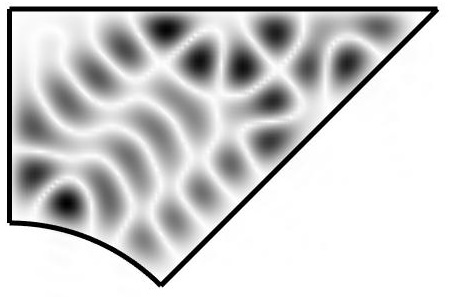
Figure 10. Symmetries of the Sinai billiard (left), desymmetrized domain embedded in a square (middle), and nodal lines of 40th eigenstate (right).

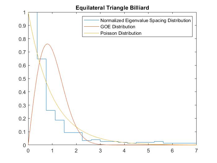
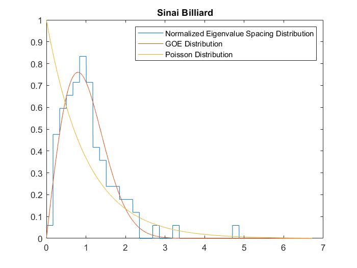
Figure 11. The eigenvalue spacings of an equilateral triangle (left) compared to those of the Sinai Billiard (right).

Spherical billiards.

Here, we consider spherical domains: octant (spherical equilateral triangle) and octant with a hole removed as shown in Figure 12. The former does not have a terminating series of desymmetrizations (so we leave it as is). However, we indeed can perform a desymmetrization on the latter, as shown. The eigenvalue distributions are compared in Figure 12. These eigenvalue statistics suggest the domains are regular and chaotic, respectively.

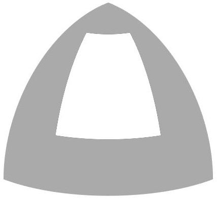
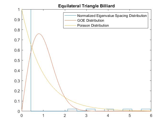
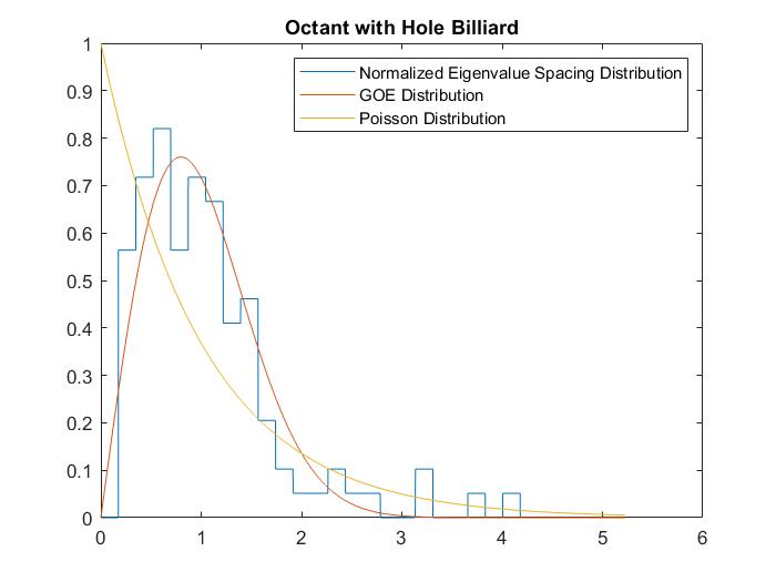
Figure 12. Spherical octant (top left), octant with hole (top middle), and desymmetrized octant with hole (top right). Their respective eigenvalue spacings (bottom).

Periodic billiards.

In Figure 13 we illustrate and compute eigenvalue spacings for two periodic domains after necessary desymmetrizing. They both have eigenvalues with low clustering and appear to take on a Poisson distribution, indicating chaotic trajectories.

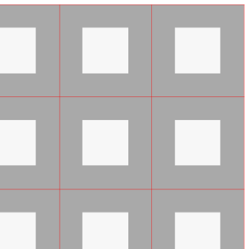
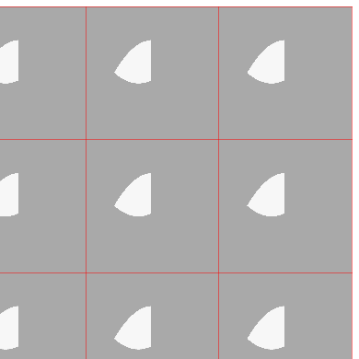
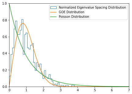
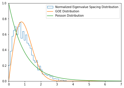
Figure 13. Four cells of two periodic domains (top) and their respective histograms of the normalized Eigenvalue Spacing Distributions for the regions obtained by desymmetrizing (bottom). The grey regions indicate $\Omega$, and we impose Dirichlet boundary conditions where they meet the white regions. The first twelve eigenfunctions for the asymmetric domain are shown in Figure 8.

6. Conclusion

The Laplace–Beltrami operator is crucial to describing many physical phenomena on manifolds, and calculation of its eigenvalues is important to many applications involving non-Euclidean media. The generalized expansion method described in this paper provides a straightforward approach to discretize the Laplace–Beltrami operator to approximate its eigenmodes and eigenvalues. We provided proofs for its spectral convergence (Theorems 7 and 9) along with various analytic and numerical examples, including its application to studying billiard problems on surfaces. Notable applications for this method exist in nonlinear systems such as the study of Kerr media and Bose-Einstein condensates where one may approximate solutions by iterating on the ground state solution of the Schrödinger equation [15, 5, 6]. Additionally, many applications exist in condensed matter physics. For example, as demonstrated in Section 5.2, this method can be used to solve for Bloch states of periodic domains defined on a lattice. Other applications include theories of 2D materials [4, 33], superconductors [9], and types of soft matter such as membranes [31].

Acknowledgement

The authors acknowledge the support from Department of Mathematics at University of Utah where this project was initialized. Elena Cherkaev acknowledges support from the U.S. National Science Foundation through grants DMS-1715680 and DMS-2111117. Dong Wang acknowledges the support from National Natural Science Foundation of China (NSFC) grant 12101524 and the University Development Fund from The Chinese University of Hong Kong, Shenzhen (UDF01001803).

References

- [1] Paolo Amore “Solving the Helmholtz equation for membranes of arbitrary shape: numerical results” In Journal of Physics A: Mathematical and Theoretical 41.26 IOP Publishing, 2008, pp. 265206
- [2] Paolo Amore “Spectroscopy of drums and quantum billiards: Perturbative and nonperturbative results” In Journal of mathematical physics 51.5 American Institute of Physics, 2010, pp. 052105
- [3] YY Atas, E Bogomolny, O Giraud and G Roux “Distribution of the ratio of consecutive level spacings in random matrix ensembles” In Physical review letters 110.8 APS, 2013, pp. 084101
- [4] Phaedon Avouris, Tony F Heinz and Tony Low “2D Materials” Cambridge University Press, 2017
- [5] W. Bao “Ground states and dynamics of multicomponent Bose–Einstein condensates” In Multiscale Modeling & Simulation 2.2, 2004, pp. 210–236 DOI: 10.1137/030600209
- [6] W. Bao and Q. Du “Computing the ground state solution of Bose–Einstein condensates by a normalized gradient flow” In SIAM Journal on Scientific Computing 25.5, 2004, pp. 1674–1697 DOI: 10.1137/s1064827503422956
- [7] Weizhu Bao “The nonlinear Schrödinger equation and applications in Bose-Einstein condensation and plasma physics” In Dynamics in models of coarsening, coagulation, condensation and quantization 9 World Scientific River Edge, NJ, USA, 2007, pp. 141–240
- [8] Alexander Harvey Barnett “Dissipation in Deforming Chaotic Billiards” Harvard University, 2000
- [9] Oleg L Berman, Yurii E Lozovik, Sergey L Eiderman and Rob D Coalson “Superconducting photonic crystals: Numerical calculations of the band structure” In Physical Review B 74.9 APS, 2006, pp. 092505
- [10] Michael V Berry “Semiclassical mechanics of regular and irregular motion” In Les Houches lecture series 36 North-Holland Amsterdam, 1983, pp. 171–271
- [11] Michael Victor Berry and Mark Wilkinson “Diabolical points in the spectra of triangles” In Proceedings of the Royal Society of London. A. Mathematical and Physical Sciences 392.1802 The Royal Society London, 1984, pp. 15–43
- [12] Timo Betcke “The generalized singular value decomposition and the method of particular solutions” In SIAM Journal on Scientific Computing 30.3 SIAM, 2008, pp. 1278–1295
- [13] Beniamin Bogosel “Efficient algorithm for optimizing spectral partitions” In Applied Mathematics and Computation 333 Elsevier BV, 2018, pp. 61–75 DOI: 10.1016/j.amc.2018.03.087
- [14] B. Bourdin, D. Bucur and É. Oudet “Optimal partitions for eigenvalues” In SIAM Journal on Scientific Computing 31.6, 2010, pp. 4100–4114 DOI: 10.1137/090747087
- [15] Jared C Bronski, Lincoln D Carr, Bernard Deconinck and J Nathan Kutz “Bose-Einstein condensates in standing waves: The cubic nonlinear Schrödinger equation with a periodic potential” In Physical Review Letters 86.8 APS, 2001, pp. 1402
- [16] S.-M. Chang, C.-S. Lin, T.-C. Lin and W.-W. Lin “Segregated nodal domains of two-dimensional multispecies Bose–Einstein condensates” In Physica D: Nonlinear Phenomena 196.3, 2004, pp. 341–361 DOI: 10.1016/j.physd.2004.06.002
- [17] Howard S Cohl and Ernie G Kalnins “Fundamental solution of the Laplacian in the hyperboloid model of hyperbolic geometry” In arXiv preprint arXiv:1201.4406, 2012
- [18] M. Conti, S. Terracini and G. Verzini “An optimal partition problem related to nonlinear eigenvalues” In Journal of Functional Analysis 198.1, 2003, pp. 160–196 DOI: 10.1016/s0022-1236(02)00105-2
- [19] O Cybulski and R Holyst “Three-dimensional space partition based on the first Laplacian eigenvalues in cells” In Physical Review E 77.5, 2008, pp. 56101 DOI: 10.1103/physreve.77.056101
- [20] Gadi Fibich “The Nonlinear Schrödinger Equation” Springer, 2015
- [21] L Fox, P Henrici and C Moler “Approximations and bounds for eigenvalues of elliptic operators” In SIAM Journal on Numerical Analysis 4.1 SIAM, 1967, pp. 89–102
- [22] David Gilbarg, Neil S Trudinger, David Gilbarg and NS Trudinger “Elliptic Partial Differential Equations of Second Order” Springer, 1977
- [23] Daniel Grieser and Svenja Maronna “Hearing the shape of a triangle” In Notices of the AMS 60.11, 2013, pp. 1440–1447
- [24] Boling Guo, Zaihui Gan, Linghai Kong and Jingjun Zhang “The Zakharov System and Its Soliton Solutions” Springer, 2016
- [25] Antoine Henrot “Extremum Problems for Eigenvalues of Elliptic Operators” Springer Science & Business Media, 2006
- [26] Jeremy G Hoskins, Vladimir Rokhlin and Kirill Serkh “On the numerical solution of elliptic partial differential equations on polygonal domains” In SIAM Journal on Scientific Computing 41.4 SIAM, 2019, pp. A2552–A2578
- [27] D Kauffman, I Kosztin and K Schulten “Expansion method for stationary states of quantum billiards” In Am. J. Phys 67, 1999, pp. 133–141
- [28] Charles Kittel, Paul McEuen and Paul McEuen “Introduction to Solid State Physics” Wiley New York, 1996
- [29] James R Kuttler and Vincent G Sigillito “Eigenvalues of the Laplacian in two dimensions” In Siam Review 26.2 SIAM, 1984, pp. 163–193
- [30] Randall J LeVeque “Numerical Methods for Conservation Laws” Springer, 1992
- [31] Jannik C Meyer, Andre K Geim, Mikhail I Katsnelson, Konstantin S Novoselov, Tim J Booth and Siegmar Roth “The structure of suspended graphene sheets” In Nature 446.7131 Nature Publishing Group, 2007, pp. 60–63
- [32] B. Osting, C.. White and É. Oudet “Minimal Dirichlet energy partitions for graphs” In SIAM J. Scientific Computing 36.4, 2014, pp. A1635–A1651 DOI: 10.1137/130934568
- [33] JT Paul, AK Singh, Zheng Dong, Houlong Zhuang, BC Revard, B Rijal, M Ashton, A Linscheid, M Blonsky and D Gluhovic “Computational methods for 2D materials: discovery, property characterization, and application design” In Journal of Physics: Condensed Matter 29.47 IOP Publishing, 2017, pp. 473001
- [34] Martin Reuter, Silvia Biasotti, Daniela Giorgi, Giuseppe Patanè and Michela Spagnuolo “Discrete Laplace–Beltrami operators for shape analysis and segmentation” In Computers & Graphics 33.3 Elsevier, 2009, pp. 381–390
- [35] S Harshini Tekur and MS Santhanam “Symmetry deduction from spectral fluctuations in complex quantum systems” In Physical Review Research 2.3 APS, 2020, pp. 032063
- [36] Gerald Teschl “Mathematical Methods in Quantum Mechanics” In Graduate Studies in Mathematics 99 American Mathematical Society Providence, RI, USA, 2009, pp. 106
- [37] Lloyd N Trefethen and Timo Betcke “Computed eigenmodes of planar regions” In Contemporary Mathematics 412 Providence, RI: American Mathematical Society, 2006, pp. 297–314
- [38] Dong Wang “An efficient unconditionally stable method for dirichlet partitions in arbitrary domains” In SIAM Journal on Scientific Computing 44.4 SIAM, 2022, pp. A2061–A2088
- [39] Dong Wang and Braxton Osting “A diffusion generated method for computing Dirichlet partitions” In Journal of Computational and Applied Mathematics 351 Elsevier BV, 2019, pp. 302–316 DOI: 10.1016/j.cam.2018.11.015
- [40] Quan Yuan and Zhiqing He “Bounds to eigenvalues of the Laplacian on L-shaped domain by variational methods” In Journal of computational and applied mathematics 233.4 Elsevier, 2009, pp. 1083–1090
- [41] Vladimir E Zakharov “Stability of periodic waves of finite amplitude on the surface of a deep fluid” In Journal of Applied Mechanics and Technical Physics 9.2 Springer, 1968, pp. 190–194