Covariant transport equation and
gravito-conductivity
in generic stationary spacetimes

Abstract

We find a near detailed balance solution to the relativistic Boltzmann equation under the relaxation time approximation with a collision term which differs from the Anderson-Witting model and is dependent on the stationary observer. Using this new solution, we construct an explicit covariant transport equation for the particle flux in response to the generalized temperature and chemical potential gradients in generic stationary spacetimes, with the transport tensors characterized by some integral functions in the chemical potential and the relativistic coldness. To illustrate the application of the transport equation, we study probe systems in Rindler and Kerr spacetimes and analyze the asymptotic properties of the gravito-conductivity tensor in the near horizon limit. It turns out that both the longitudinal and lateral parts (if present) of the gravito-conductivity tend to be divergent in the near horizon limit. In the weak field limit, our results coincide with the non-relativistic gravitational transport equation which follows from the direct application of the Drude model.

1 Introduction

Transport equations for macroscopic systems under the influence of external fields are critical in understanding non-equilibrium processes. For electron gas in solid state physics, the external fields can be electromagnetic field and/or temperature gradient. For compact stars and accretions around black holes, the relativistic gravitational field must be taken into consideration. In the recent years, there has been an increasing interest in studying the evolution of kinetic gases in the vicinity of black holes. On the one hand, the macroscopic properties of near horizon systems are likely to be connected with thermodynamic effects of gravity. On the other hand, the rotating plasma surrounding supermassive black holes has been revealed by Event Horizon Telescope Collaboration [1]. Motivated by these astrophysical scenarios, it is necessary to dwell on some more details of the transport phenomena in the strong gravity regime.

Kinetic theory has long been used for constructing transport equations. In the early stages of the universe and in the near horizon region, gravity is so strong that the relativistic effect becomes important. In this situation, a relativistically covariant approach is needed. Such a systematic approach is known as the relativistic kinetic theory (RKT) and could be dated back to 1911 [2]. The modern geometrical description of specially relativistic kinetic theory is formulated in [3], which is fundamental for the generalization to curved spacetime backgrounds [4, 5, 6]. Renewed interests in this area arise following Refs.[7, 8, 9], where RKT has been respectively applied to the study of the quark-gluon plasma and heavy ion collisions [10, 11, 12, 13, 14, 15, 16, 17, 18, 19], the early Universe [20, 21, 22, 23, 24, 25, 26, 27, 28, 29] and astrophysics[30, 31, 32, 33], particularly accretion around black holes[9, 33, 34, 35]. The covariant formalism also led to the development of relativistic thermodynamics [36, 37].

The aim of the present work is to provide a covariant formulation for transport phenomena in curved spacetimes. There have been studies about the gravitational effects on the transport of conserved charge, heat and momentum [38, 40, 39]. The major difference between the present work and the previous ones lies in that we emphasize the importance of the observer, and that our collision model is independent of Landau frame. The reason for stressing the important role of observers lies as follows. As we have pointed out in [41], in relativistic physics, physical laws are independent of the choice of coordinate system, whilst the values of physical observables are observer dependent. In the description of relativistic transport phenomena, the transport equation encodes the underlying physical law which needs to be described in a covariant formalism. On the other hand, the values of the relevant transport coefficients — although also need to be tensorial objects — describe the phenomenological properties of concrete systems which depend on the choice of observer. As will be seen in the main texts below, the proper velocity of the stationary observer is crucial when modeling the collision term and interpreting the kinetic tensor.

Another difference of the present work with previous ones is that the lateral transport in our framework can be clearly separated from the longitudinal transport. One may think that the lateral effects are negligibly small as compared to the longitudinal effects. This may be a truth in some cases, but not always. For instance, around rapidly spinning black holes, the lateral effects are at least equally as important as the longitudinal effects.

For simplicity, we will work on the assumption that the gaseous (or fluid) system is consisted of massive neutral particles and is regarded as a probe system.

2 GEM field and the gravitational Hall coefficient under post-Newtonian approximation

In this section, we work within the post-Newtonian limit, i.e. when the gravitational field is weak, and the motion of the source is slow but still taken into consideration. In this limit, the gravitational field can be described by small perturbations $h_{\mu\nu}$ around Minkowski metric. When all the nonlinear terms in $h_{\mu\nu}$ are neglected, there will be an analogy between Einstein equations under de Donder gauge and the Maxwell equation under Lorenz gauge. In 4-dimensional spacetimes, such an analogy is known as the linear gravito-electromagnetism (GEM) [42, 43, 44, 45]. The solution of the linearized Einstein equation suggests that, up to $\mathcal{O}(c^{-2})$, we can write the metric as

$$\mathrm{d}s^{2}=-c^{2}\Big{(}1+\frac{2\phi}{c^{2}}\Big{)}\mathrm{d}t^{2}+\frac{4}{c}\bm{A}\cdot\mathrm{d}\bm{x}\,\mathrm{d}t+\Big{(}1-\frac{2\phi}{c^{2}}\Big{)}\delta_{ij}\mathrm{d}x^{i}\mathrm{d}x^{j},$$ (1)

where $i,j=1,2,3$, $\phi=h_{00}/2c^{2}$ is the scalar potential and $A_{i}=h_{0i}/2c^{2}$ is the vector potential. For slowly varying source, the gravito-electric (GE) field and the gravito-magnetic (GM) field become $\bm{E}^{(g)}=-\nabla\phi$ and $\bm{B}^{(g)}=\nabla\times\bm{A}$, which satisfy a set of equations analogous to the Maxwell equations in 3-vector formulation.

Another important aspect of the linear GEM framework lies in the equation of motion of a test particle. In non-relativistic limit, the proper velocity of the test particle is approximately $u^{\alpha}\approx(c,\bm{v})$, and up to ${\mathcal{O}}(c^{-1})$ the geodesic equation in terms of GE and GM reduces to Lorentz-force-like equation

$$\frac{\mathrm{d}\bm{v}}{\mathrm{d}t}=\bm{E}^{(g)}+2\,\frac{\bm{v}}{c}\times\bm{B}^{(g)},$$ (2)

as a simple application of eq.(2), we can now follow the Drude model of traditional Hall effect and introduce a linear friction term $-\bm{v}/\tau$ to the RHS, which is due to scattering between particles, and the scattering time $\tau$ is the average time between collisions. When the particle becomes equilibrated, we have roughly $\mathrm{d}\bm{v}/\mathrm{d}t=0$. In this case, the particle flow $\bm{j}=n\bm{v}$ is related to external force $\bm{E}^{(g)}$ by

$$\mathcal{R}^{(g)}\bm{j}-\mathcal{R}^{(g)}_{H}\bm{j}\times\bm{B}^{(g)}=\bm{E}^{(g)},$$ (3)

where $\mathcal{R}^{(g)}=1/n\tau$ is the gravitational resistance and $\mathcal{R}^{(g)}_{H}=2/nc$ is the gravitational Hall coefficient for neutral systems. This analogy is clear and instructive, but the Drude model is highly dependent on the Lorentz-force-like equation, therefore only applies to weak gravitational field.

In the rest of this work, we will generalize the transport equation to generic stationary spacetime backgrounds in a fully covariant form and calculate the gravitational conductivity for neutral systems as an example case for applications.

3 Relativistic Boltzmann equation and approximate solution

Before proceeding, let us mention that, in ordinary electrodynamics, different observers should observe different electric ($\bm{E}$) and magnetic ($\bm{B}$) fields, which is known as the Faraday effect. Likewise, The GE and GM fields must also be observer dependent. The description presented in the last section did not show this observer dependence, because a specific observer, i.e. the static observer in the Minkowski background spacetime, is implicitly adopted.

In the following, we will try to establish a fully covariant formalism for the relativistic transport equations. For this purpose, we need to bring back the explicit observer dependence. It turns out that the stationary observer is best suited for our investigation. Therefore we shall assume that the spacetime is stationary (i.e. there exists a timelike Killing vector field).

From now on, we will be working in natural units with $c=h=k_{\rm B}=1$. We introduce a generic observer $\mathcal{O}$ with proper velocity $Z^{\mu}$ (with $Z^{\mu}Z_{\mu}=-1$) and the observer dependence of the GE and GM fields are best illustrated by their expressions in terms of $Z^{\mu}$, i.e.

$$E^{(g)}_{\mu}=-Z^{\nu}\nabla_{\nu}Z_{\mu},\qquad B^{(g)}_{\mu\nu}=\frac{1}{2}\nabla_{[\alpha}Z_{\beta]}\Delta^{\alpha}{}_{\mu}\Delta^{\beta}{}_{\nu},$$ (4)

where $\Delta_{\mu\nu}=g_{\mu\nu}+Z_{\mu}Z_{\mu}$ is the normal projection tensor associated with the observer $\mathcal{O}$. It should be mentioned that the covariant GE field $E^{(g)}_{\mu}$ is proportional to the proper acceleration of the observer $\mathcal{O}$. The GM field represented in vector form can be introduced as

$$B^{(g)\mu}={\color[rgb]{0,0,0}-}\Delta^{\mu}{}_{\nu}\varepsilon^{\nu\alpha\beta}B^{(g)}_{\alpha\beta},$$

where $\varepsilon^{\nu\alpha\beta}$ is the Levi-Civita tensor.

Now let us proceed with a brief review of the relativistic kinetic theory for a system composed of neutral particles moving in curved spacetime. The macroscopic state of the system is described by the particle number flow $N^{\mu}$, the energy momentum tensor $T^{\mu\nu}$ and the entropy current $S^{\mu}$. These quantities are primary in the fluid description of macroscopic systems [46]. In the absence of external field besides gravity, one has

$$\nabla_{\mu}N^{\mu}=0,\qquad\nabla_{\mu}T^{\mu\nu}=0,\qquad\nabla_{\mu}S^{\mu}\geqslant 0.$$ (5)

The expressions for $N^{\mu}$, $T^{\mu\nu}$ and $S^{\mu}$ in terms of other macroscopic observables such as temperature $T$, chemical potential $\mu$ and entropy density $s$ are called constitutive relations. It is important to keep in mind that $T$, $\mu$, $s$ and therefore the constitutive relations are observer dependent, but the above primary macroscopic quantities are not, since they have microscopic definitions. In standard relativistic kinetic theory, the primary macroscopic quantities are expressed as integrations over one-particle distribution function (1PDF),

$$N^{\mu}=\int\bm{\varpi}p^{\mu}f,\qquad T^{\mu\nu}=\int\bm{\varpi}p^{\mu}p^{\nu}f,$$ (6)

$$S^{\mu}=-\int\bm{\varpi}p^{\mu}\left[f\log f-\varsigma^{-1}\left(1+\varsigma f\right)\log\left(1+\varsigma f\right)\right],$$ (7)

where $\varsigma=0,+1,-1$ respectively corresponds to the non-degenerate, bosonic and fermionic cases, $\bm{\varpi}=\mathfrak{g}\frac{\sqrt{g}}{p_{0}}(\mathrm{d}p)^{d}$ is the invariant volume element in the momentum space with $\mathfrak{g}$ being the intrinsic degeneracy factor for individual particles in the system, and the spacetime dimension is chosen to be $(d+1)$. The above definitions are valid for systems away from equilibrium. Therefore, in kinetic theory, we can ask whether the equilibrium state can be achieved in curved spacetime, and find the constraints for the spacetime metric to embed an equilibrium system. Since the primary macroscopic quantities are totally determined by the 1PDF, the relativistic Boltzmann equation (RBE) is then of fundamental importance

$$\mathscr{L_{\mathcal{H}}}f=\mathcal{C}(f),$$ (8)

where $\displaystyle\mathscr{L_{\mathcal{H}}}=p^{\mu}\frac{\partial}{\partial x^{\mu}}-\Gamma^{\mu}{}_{\alpha\beta}p^{\alpha}p^{\beta}\frac{\partial}{\partial p^{\mu}}$ is the Liouville vector field on the tangent bundle of the spacetime.

There are two-fold complexities in the RBE, which make it challenging to find an exact solution. On the left hand side, the spacetime geometry is encoded in the Liouville vector field, however the spacetime geometry itself can only be determined by solving the Einstein equation with the energy-momentum tensor acting as the source, but to define the energy-momentum tensor one needs the 1PDF which is the sought-for solution of the RBE. Therefore, the RBE and Einstein equation together constitute a coupled system of differential-integral equations which is extremely difficult to solve. On the right hand side, the exact expression for the collision integral $\mathcal{C}(f)$ requires the knowledge of precise form of the transition matrix for two particle scattering.

Fortunately, most of the difficulties can be overcome by adopting the probe limit and by making certain simplifications for the collision integral by assuming certain symmetries. The most commonly used assumption is that the transition matrix obeys time reversal symmetry. Under this assumption, the vanishing of entropy production rate indicates that $\mathcal{C}(f)=0$, which is known as the detailed balance condition. As a result, the RBE reduces to the Liouville equation, and the solution is the detailed balance distribution

$$\bar{f}=\frac{1}{\mathrm{e}^{\bar{\alpha}-\bar{\mathcal{B}}_{\mu}p^{\mu}}-\varsigma},$$ (9)

where $\bar{\alpha}$ and $\bar{\mathcal{B}}^{\mu}$ are independent of momentum, $\bar{\alpha}$ is a constant scalar in spacetime manifold and $\bar{\mathcal{B}}^{\mu}$ is a Killing vector field. Please keep in mind that quantities with an over bar are evaluated under detailed balance. On account of the energy conditions for $T^{\mu\nu}$, we only study the fluid system where $\bar{\mathcal{B}}^{\mu}$ is timelike.

Although the primary tensor objects $N^{\mu},T^{\mu\nu},S^{\mu}$ are observer independent, their values under detailed balance are best expressed in terms of the proper velocity of the comoving observer. Let us recall that an observer whose proper velocity is proportional to the timelike Killing vector field is stationary, while an observer whose proper velocity is a timelike eigenvector field of $T^{\mu\nu}$ is comoving. Since we have already assumed that $\bar{\mathcal{B}}^{\mu}$ is timelike and Killing, we can determine the proper velocity $Z^{\mu}$ of the stationary observer via $\bar{\mathcal{B}}^{\mu}=\bar{\beta}Z^{\mu}$ and $Z^{\mu}Z_{\mu}=-1$. In terms of $Z^{\mu}$ and its corresponding projection tensor $\Delta_{\mu\nu}$, the primary tensor objects for a system consisted of massive particles of mass $m$ under detailed balance are evaluated to be

$$\bar{N}^{\mu}=\mathfrak{g}m^{d}\mathcal{A}_{d-1}\bar{J}_{d-1,1}\,Z^{\mu},$$ (10)

$$\bar{T}^{\mu\nu}=\mathfrak{g}m^{d+1}\mathcal{A}_{d-1}\left(\bar{J}_{d-1,2}\,Z^{\mu}Z^{\nu}+\frac{1}{d}\bar{J}_{d+1,0}\,\Delta^{\mu\nu}\right),$$ (11)

$$\bar{S}^{\mu}=\mathfrak{g}m^{d}\mathcal{A}_{d-1}\left(\bar{\alpha}\bar{J}_{d-1,1}+\bar{\zeta}\bar{J}_{d-1,2}+\frac{\bar{\zeta}}{d}\bar{J}_{d+1,0}\right)Z^{\mu},$$ (12)

where $\mathcal{A}_{d-1}$ is the area of the $(d-1)$-dimensional unit sphere, and $\bar{J}_{nm}$ is the following function in $(\bar{\alpha},\bar{\zeta})$, wherein $\bar{\zeta}=\bar{\beta}m$ is known as the relativistic coldness,

$$\bar{J}_{nm}=J_{nm}(\bar{\alpha},\bar{\zeta},\varsigma)=\int_{0}^{\infty}\frac{\sinh^{n}\vartheta\cosh^{m}\vartheta}{\mathrm{e}^{\bar{\alpha}+\bar{\zeta}\cosh\vartheta}-\varsigma}\mathrm{d}\vartheta.$$

As usual, the parameters $\bar{\alpha},\bar{\beta}$ are related to the chemical potential $\bar{\mu}$ and temperature $\bar{T}$ measured by the comoving observer via

$$\bar{\alpha}=-\bar{\mu}/\bar{T},\qquad\bar{\beta}=1/\bar{T}.$$

A key feature hidden in the above results is that $\bar{N}^{\mu}$, $\bar{S}^{\mu}$ and the eigenvector of $\bar{T}^{\mu\nu}$ are collinear, and the unique timelike eigenvector of $\bar{T}^{\mu\nu}$ coincides with $Z^{\mu}$. Therefore, the stationary observer in this case is automatically comoving. Please be reminded that this feature is present only in the presence of detailed balance. For systems away from detailed balance, there is no first principle definition for comoving observer. Therefore, in the following, we will only consider stationary observers, and the results will be presented in a covariant way.

In the eyes of a stationary observer, the temperature $\bar{T}$ and the chemical potential $\bar{\mu}$ under detailed balance satisfy

$$\mathcal{D}_{\nu}\bar{T}\equiv\nabla_{\nu}\bar{T}+\bar{T}\,Z^{\sigma}\nabla_{\sigma}Z_{\nu}=0,\qquad\mathcal{D}_{\nu}\bar{\mu}\equiv\nabla_{\nu}\bar{\mu}+\bar{\mu}\,Z^{\sigma}\nabla_{\sigma}Z_{\nu}=0.$$

We see that due to the Tolman-Ehrenfest effect and the Klein effect, chemical potential gradient and the temperature gradient alone can be no longer viewed as thermodynamic forces in gravitation field. In the above modification, we have defined the generalized temperature gradient $\mathcal{D}_{\nu}T$ and the generalized chemical potential gradient $\mathcal{D}_{\nu}\mu$ which are responsible for thermodynamic forces.

Now we turn on external field by setting $\mathcal{D}_{\nu}T,\mathcal{D}_{\nu}\mu\neq 0$, while still taking the probe limit and keeping the spacetime metric fixed. In this case, $\bar{\alpha},\bar{\beta}$ will be replaced by $\alpha,\beta$ which are slightly different from the former, i.e. $\bar{\alpha}\to\alpha=\bar{\alpha}+\delta\alpha$, $\bar{\beta}\to\beta=\bar{\beta}+\delta\beta$. In particular, there is no reason to take $\alpha$ as a constant. As a result, $\mathcal{B}^{\mu}\equiv\beta Z^{\mu}$ is no longer Killing, although $Z^{\mu}$ remains to be the proper velocity of the stationary observer.

Since we are now considering cases away from detailed balance, the 1PDF $f$ should differ from $\bar{f}$. If the deviation from detailed balance is not too severe, we can reasonably assume that the zeroth order approximation to the 1PDF takes the form

$$f^{(0)}=\frac{1}{\mathrm{e}^{\alpha-\mathcal{B}_{\mu}p^{\mu}}-\varsigma}$$ (13)

and that the deviation of the full 1PDF $f$ from $f^{(0)}$ can be treated as a perturbative modification.

In order to obtain a better approximate solution to the full RBE, one needs to simplify the collision integral by replacing the integral with some algebraic expression while maintaining its basic symmetries. This kind of simplification is known as relaxation time approximation and its concrete realizations are known as collision models. In non-relativistic framework, the most widely known collision model is the Bhatnagar-Gross-Krook (BGK) model [47] which maintains the conservation of mass, momentum and energy. The direct application of BGK model in the relativistic case is called Marle-BGK model [48] which seems to be oversimplified, since the relaxation time becomes unbounded in ultra-relativistic limit. This problem was pointed out by Anderson and Witting who successively proposed an alternative, adapted collision model which is referred to as Anderson-Witting (AW) model [38]. In AW model, Landau frame must be preassigned to guarantee the conservation laws for particle flow and energy-momentum tensor. However, in the present work, when external field is turned on, the conservation laws becomes less important, instead, the generalized chemical potential and temperature gradients must be taken into account. In this case, the stationary observer plays a prominent role. On the one hand, $Z^{\mu}$ is used to define $\mathcal{D}_{\nu}T$ and $\mathcal{D}_{\nu}\mu$. On the other hand, when back reaction is neglected, $Z^{\mu}$ is independent of the perturbation. Following the above considerations, we propose the following collision model

$$\mathscr{L}_{\mathcal{H}}f=-\frac{\varepsilon}{\tau}(f-f^{(0)})=\frac{Z_{\mu}p^{\mu}}{\tau}(f-f^{(0)}),$$ (14)

where $\varepsilon=-Z_{\mu}p^{\mu}$ represents the energy of a single particle measured by the stationary observer, and $\tau$ is the time scale for the system to restore detailed balance. As the external fields $\mathcal{D}_{\nu}T$ and $\mathcal{D}_{\nu}\mu$ are turned on, $Z^{\mu}$ does not necessarily coincide with the proper velocity of the fluid element in the Landau frame, therefore, this collision model is different from AW model.

The desired solution for eq.(14) is found to be $f=f^{(0)}+\delta f$, where the modification $\delta f$ arises due to the presence of the generalized temperature gradient and generalized chemical potential gradient. Up to $\mathcal{O}(\tau^{2})$, the explicit expression for $\delta f$ reads

$$\delta f=\frac{\tau}{\varepsilon}\frac{\partial f^{(0)}}{\partial\varepsilon}p^{\mu}\left(\delta_{\mu}{}^{\nu}+\frac{\tau}{\varepsilon}\Delta^{\alpha}{}_{\mu}\nabla_{[\alpha}p_{\beta]}\,\Delta^{\beta\nu}\right)\left(\mathcal{D}_{\nu}\mu+\frac{\varepsilon-\mu}{T}\mathcal{D}_{\nu}T\right).$$ (15)

This equation is one of our main results and the recursive procedure for obtaining this approximate solution is given in appendix A.

4 Transport equations and gravito-conductivity

The approximate solution to the RBE obtained in the last section allows us to study various transport equations in a covariant manner. To illustrate such applications, we will now take the particle number flow $N^{\mu}$ as an example and leave the detailed study about the transport behaviors for $T^{\mu\nu}$ and $S^{\mu}$ for later works.

According to the definition (5) for the particle number flow, we have

$$N^{\mu}=\left[N^{(0)}\right]^{\mu}+\delta N^{\mu}=\int\bm{\varpi}p^{\mu}f^{(0)}+\int\bm{\varpi}p^{\mu}\delta f.$$

The first part of $N^{\mu}$, i.e. $\left[N^{(0)}\right]^{\mu}$, is collinear with $Z^{\mu}$, hence only a scalar density $n^{(0)}=-Z_{\mu}\left[N^{(0)}\right]^{\mu}$ is encoded in this part of the particle number flow, which reads

$$n^{(0)}=\mathfrak{g}m^{d}\mathcal{A}_{d-1}J_{d-1,1},$$ (16)

wherein $J_{d-1,1}$ is like $\bar{J}_{d-1,1}$ but with $\bar{\alpha},\bar{\zeta}$ replaced by $\alpha,\zeta$, and therefore $n^{(0)}$ is slightly different from the particle number density $\bar{n}$ under the detailed balance condition. The second part of the particle number flow, i.e. $\delta N^{\mu}$, is not collinear with $Z^{\mu}$. One can project $\delta N^{\mu}$ onto parallel and orthogonal directions with respect to $Z^{\mu}$, where the parallel projection $\delta n\equiv-Z_{\mu}\delta N^{\mu}$ contributes a higher order correction to the particle number density $n=n^{(0)}+\delta n$, while the orthogonal projection gives rise to the following transport equation for the particle number, which reads (see appendix B for details)

$$j^{\mu}\equiv\Delta^{\mu}{}_{\nu}\delta N^{\nu}=-\tau\mathfrak{g}{m}^{d-1}\Big{(}\sigma^{\mu\nu}\mathcal{D}_{\nu}\mu+\kappa^{\mu\nu}\mathcal{D}_{\nu}T\Big{)},$$ (17)

where the dimensionless factors $\sigma^{\mu\nu}$ and $\kappa^{\mu\nu}$ in the transport tensors are given by

$$\sigma^{\mu\nu}=\frac{\mathcal{A}_{d-1}}{d}\left(\Delta^{\mu\nu}+2\tau B^{(g)\mu\nu}\right)\zeta\mathcal{J}_{d+1,-1},\quad\kappa^{\mu\nu}=\sigma^{\mu\nu}\left(\alpha+\zeta\frac{\mathcal{J}_{d+1,0}}{\mathcal{J}_{d+1,-1}}\right),$$

in which $\mathcal{J}_{nm}$ is defined as

$$\mathcal{J}_{nm}(\alpha,\zeta,\varsigma)=J_{nm}(\alpha,\zeta,\varsigma)+\varsigma\int_{0}^{\infty}\frac{\sinh^{n}\vartheta\cosh^{m}\vartheta}{\left(\mathrm{e}^{\alpha+\zeta\cosh\vartheta}-\varsigma\right)^{2}}\mathrm{d}\vartheta.$$

The covariant transport equation (17) is valid for any probe system in any stationary spacetime, even in the strong field regime. Therefore, it can be used for describing near horizon particle transport. Let us remark that $\sigma^{\mu\nu}$ and $\kappa^{\mu\nu}$ differ from each other only by a scalar factor. Therefore, it suffices to consider only the gravito-conductivity characterized by $\sigma^{\mu\nu}$ in the following context (the actual gravito-conductivity differs from $\sigma^{\mu\nu}$ by a constant factor $-\tau\mathfrak{g}{m}^{d-1}$, but we shall slightly abuse the terminology and simply refer to $\sigma^{\mu\nu}$ as gravito-conductivity). The ratio between $\kappa^{\mu\nu}$ and $\sigma^{\mu\nu}$ may be defined as the gravitational Seebeck coefficient.

Due to phenomenological considerations, it may be helpful to decompose the particle flux (17) into longitudinal and lateral parts with respect to the natural orthogonal frame carried by the stationary observer. For better understanding, let us rewrite eq.(17) in the orthonormal basis $\{e_{\hat{\alpha}}{}^{\mu}\}$, $\eta_{\hat{\alpha}\hat{\beta}}=g_{\mu\nu}e_{\hat{\alpha}}{}^{\mu}e_{\hat{\beta}}{}^{\nu}$, where $\eta_{\hat{\alpha}\hat{\beta}}$ represents the Minkowski metric in orthogonal basis and $e_{\hat{0}}{}^{\mu}\equiv Z^{\mu}$. In this basis, the symmetric and the antisymmetric parts of $\sigma^{\mu\nu}$ become, respectively,

$$\sigma_{\|}^{\hat{a}\hat{b}}=\frac{\mathcal{A}_{d-1}}{d}\zeta\mathcal{J}_{d+1,-1}\delta^{\hat{a}\hat{b}},\qquad\sigma_{\bot}^{\hat{a}\hat{b}}=2\tau\frac{\mathcal{A}_{d-1}}{d}\zeta\mathcal{J}_{d+1,-1}B^{(g)\hat{a}\hat{b}},$$

where $\hat{a},\,\hat{b}=1,2,\cdots,d$. Naturally, $\sigma_{\|}^{\hat{a}\hat{b}}$ and $\sigma_{\bot}^{\hat{a}\hat{b}}$ obey Onsager’s reciprocal relations and, respectively, characterize the longitudinal (or, diagonal ) and lateral (i.e. Hall ) gravito-conductivities. Let us stress once again that the gravito-conductivity presented as above is independent of the choice of background geometry and is valid in any stationary spacetimes. The only effect of the choice of background geometry is carried by the redshifts of the relativistic coldness and the chemical potential through Tolman-Ehrenfest and Klein effects.

5 Example cases and weak field limit

5.1 Example cases

As concrete example cases, let us analyze the gravitational conductivity under two nontrivial spacetime backgrounds. The first example case is the $(d+1)$-dimensional Rindler spacetime with line element

$$\mathrm{d}s^{2}=g_{\mu\nu}\mathrm{d}x^{\mu}\mathrm{d}x^{\nu}=-\kappa^{2}x^{2}\mathrm{d}t^{2}+\mathrm{d}x^{2}+\mathrm{d}\Sigma^{2}_{d-1},$$ (18)

where $\mathrm{d}\Sigma^{2}_{d-1}$ denotes the line element of $(d-1)$-dimensional Euclidean space. The above Rindler spacetime contains an accelerating horizon located at $x_{h}=0$. For a gaseous system of massive particles residing in this accelerating spacetime, the coldness will be shifted differently at different spatial places due to Tolman-Ehrenfest effect, i.e. $\zeta\sim\kappa x$. In the near horizon limit, we have $\zeta\to 0$ and asymptotically $\mathcal{J}_{d+1,-1}\sim\zeta^{-d}$ (see appendix C). Therefore, we conclude that the longitudinal part of the gravito-conductivity tensor $\sigma_{\|}^{\hat{a}\hat{b}}$ tends to be divergent in the near horizon limit provided $d>2$, and it converges only when the spacetime dimension is $1+1$.

In the above example, the GM field defined in eq.(4) and consequently the lateral part of the conductivity tensor is identically zero. In order to demonstrate the lateral part, let us take the Kerr black hole spacetime as the background. For a gaseous system co-rotating with the spacetime, the coldness will be shifted as

$$\zeta\sim\sqrt{1-\dfrac{r_{g}r}{r^{2}+a^{2}\cos^{2}\theta}},$$

where $r_{g}$ is gravitational radius and $a$ is the Kerr parameter. In this case $\zeta$ tends to be zero at the ergosphere, and in this limit we have asymptotically $\mathcal{J}_{4,-1}(\alpha,\zeta,\varsigma)\sim\zeta^{-3}$. As a result, the longitudinal conductivity tensor tends to be divergent at the ergosphere. For the same reason, the lateral (antisymmetric) part of the conductivity tensor also tends to be divergent at the ergosphere. The behaviors of $\sigma_{\bot}^{\hat{1}\hat{3}}$ and $\sigma_{\bot}^{\hat{2}\hat{3}}$ in the near horizon limit are graphically depicted in Fig.1.

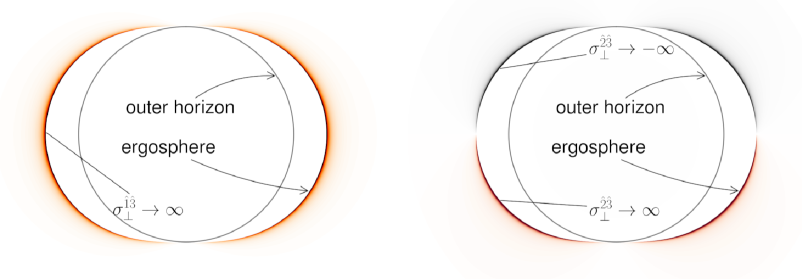
Figure 1: $\sigma_{\bot}^{\hat{1}\hat{3}}$ and $\sigma_{\bot}^{\hat{2}\hat{3}}$ : darker colors represent bigger amplitudes

5.2 Weak field limit

As an alternative justification of the results presented in the last section, let us now consider the weak field limit. In this limit, the stationary observer automatically falls back to the static observer in the Minkowski background.

For simplicity, we will consider only the cases with $\mathcal{D}_{\nu}T=0$, under which condition the covariant transport equation becomes

$$j^{\mu}=-{\tau}{\mathfrak{g}}m^{d-1}\frac{\mathcal{A}_{d-1}}{d}\zeta\mathcal{J}_{d+1,-1}\left(\Delta^{\mu\nu}+2\tau B^{(g)\mu\nu}\right)\mathcal{D}_{\nu}\mu.$$ (19)

Multiplying $\Delta_{\mu\nu}-2\tau B^{(g)}_{\mu\nu}$ on both hand sides and neglecting terms of order ${\mathcal{O}}(\tau^{3})$, we get

$$j^{\mu}\left(\Delta_{\mu\nu}-2\tau B^{(g)}_{\mu\nu}\right)=-{\tau}{\mathfrak{g}}m^{d-1}\frac{\mathcal{A}_{d-1}}{d}\zeta\mathcal{J}_{d+1,-1}\Delta_{\nu}{}^{\alpha}\mathcal{D}_{\alpha}\mu=-\frac{\tau}{m}\frac{n^{(0)}}{d}\frac{\zeta\mathcal{J}_{d+1,-1}}{J_{d-1,1}}\Delta_{\nu}{}^{\alpha}\mathcal{D}_{\alpha}\mu,$$ (20)

where, in the last step, eq.(16) has been used.

Moreover, if $\nabla_{\nu}\mu=0$, the generalized chemical potential gradient becomes proportional to the pure GE field, i.e. $\mathcal{D}_{\nu}\mu=-\mu E^{(g)}_{\nu}$. In this case, the transport equation can be rearranged in the form

$$\mathcal{R}^{(g)}j_{\nu}-\mathcal{R}^{(g)}_{H}j^{\mu}B^{(g)}_{\mu\nu}=E^{(g)}_{\nu},$$ (21)

which looks very similar to eq.(3), wherein gravitational resistance and the gravitational Hall coefficient are respectively

$$\mathcal{R}^{(g)}=\frac{d\,J_{d-1,1}}{\zeta\mathcal{J}_{d+1,-1}}\frac{m}{\mu}\frac{1}{n^{(0)}\tau},\qquad\mathcal{R}^{(g)}_{H}=\frac{d\,J_{d-1,1}}{\zeta\mathcal{J}_{d+1,-1}}\frac{m}{\mu}\frac{2}{n^{(0)}}.$$

For $d=3$ and taking the non-relativistic limit $\zeta\gg 1$, we have ${3\,J_{2,1}}\approx\zeta\mathcal{J}_{4,-1}$, $\mu\approx m$. In this case, eq.(21) becomes precisely eq.(3), with

$$\mathcal{R}^{(g)}\approx\frac{1}{n^{(0)}\tau},\qquad\mathcal{R}^{(g)}_{H}\approx\frac{2}{n^{(0)}},$$

which recovers the results mentioned near the end of Section 2.

6 Summary

Transport phenomena under the influence of gravity are among the most important macroscopic effects which are relevant to the formation and development of astrophysical structures. In the presence of gravito-electromagnetism, both longitudinal and lateral transports could arise. In the weak field regime, one can adopt the post-Newtonian approximation and make use of the the Drude model to describe the gravito-transport phenomena, and in such cases the lateral gravito-transport effect could be negligibly small. However, in the strong field regime, the lateral transport effect may be non-negligible, and even likely to be dominated. Therefore, a fully covariant approach for the gravito-transport phenomena is needed.

In this work, we provided a fully covariant approach for the gravito-transport equation in the framework of relativistic kinetic theory. The key step is the introduction of a novel collision model which is different from the well-known Anderson-Witting model and greatly facilitated the simplification of the relativistic Boltzmann equation. In this construction, the proper velocity of the stationary observer played an important role. Taking advantage of the novel collision model, an approximate near detailed balance solution (15) for the relativistic Boltzmann equation is obtained for a system of massive neutral particles moving in a generic stationary spacetime.

As an application of the solution (15), we calculated the particle flux and derived one of the transport equations. We found that the gravitational conductivity tensor is temperature dependent, which is in turn affected by the Tolman-Ehrenfest effect. Finally, we considered some concrete examples. For neutral fluid in Rindler spacetime, only longitudinal flux exists and the gravito-conductivity is divergent at the accelerating horizon. While for neutral fluid co-rotating with Kerr spacetime, both the longitudinal and the lateral parts of the gravito-conductivity are present and they both tend to be divergent at the ergosphere. Whether the divergence of the particle flux at the infinite redshift surfaces could be considered as a new kind of superconductivity deserves further study. Even though, it seems that the behaviors of macroscopic systems in the presence of gravity at high temperatures are quite similar to that of ordinary macroscopic systems in the absence of gravity at low temperatures. This similarity has also shown up in the recent study about the thermodynamic behaviors of AdS black holes in the high temperature limit [49].

As a final justification of the covariant formalism, we also considered the weak field limit and find good agreement with the result that follows from the post Newtonian approximation with the use of the Drude model.

Appendices

Appendix A Solution to equation (14)

In this section, we present a recursive solution to (14). In order to find the modification $\delta f$, let us first decompose the LHS of the RBE into

$$\mathscr{L}_{\mathcal{H}}f =p^{\sigma}\partial_{\sigma}f-\frac{1}{2}g^{\mu\sigma}p^{\alpha}p^{\beta}\partial_{\alpha}g_{\beta\sigma}\frac{\partial f}{\partial p^{\mu}}+mF^{(p)\mu}{}_{\nu}\,p^{\nu}\frac{\partial f}{\partial p^{\mu}}.$$ (22)

where $F^{(p)}_{\mu\nu}$ is defined as

$$F^{(p)}_{\mu\nu}=\frac{1}{m}\nabla_{[\mu}\,p_{\nu]}=\frac{1}{2m}(\nabla_{\mu}p_{\nu}-\nabla_{\nu}p_{\mu}).$$

It is customary to decompose the tensor $F^{(p)}_{\mu\nu}$ into its “electric” and “magnetic” parts (as observed by the observer $Z^{\mu}$),

$$F^{(p)}_{\mu\nu}=\big{(}Z_{\mu}E^{(p)}_{\nu}-E^{(p)}_{\mu}Z_{\nu}\big{)}+B^{(p)}_{\mu\nu},$$ (23)

where

$$E^{(p)}_{\mu}=F^{(p)}_{\mu\nu}Z^{\nu},\qquad B^{(p)}_{\mu\nu}=F^{(p)}_{\alpha\beta}\Delta^{\alpha}{}_{\mu}\Delta^{\beta}{}_{\nu}.$$ (24)

Let us remind that $B^{(p)}_{\mu\nu}$ should not be confused with $B^{(g)}_{\mu\nu}$ defined in eq.(4). Inserting the collision model (14) into the RHS of the RBE, we get

$$f =f^{(0)}-\frac{\tau}{\varepsilon}\mathscr{L}_{\mathcal{H}}f.$$ (25)

The approximate solution to eq.(25) can be obtained through a recursive procedure. At the first order in $\tau$, we can write

$$f \approx f^{(0)}-\frac{\tau}{\varepsilon}\mathscr{L}_{\mathcal{H}}f^{(0)}=f^{(0)}+\frac{\tau}{\varepsilon}p^{\nu}\mathscr{F}^{(0)}_{\nu}\frac{\partial f^{(0)}}{\partial\varepsilon},$$ (26)

where

$$\mathscr{F}^{(0)}_{\nu} =\mathcal{D}_{\nu}\mu+\frac{\varepsilon-\mu}{T}\mathcal{D}_{\nu}T.$$ (27)

At this level of the approximation, the magnetic part $B^{(p)}_{\mu\nu}$ of the tensor $F^{(p)}_{\mu\nu}$ makes no contribution, because $Z^{\mu}\Delta_{\mu\nu}$ is identically zero. In order to get a refined approximate solution which encodes the effects of the magnetic parts, we must not replace all occurrences of $f$ in the expression $\mathscr{L}_{\mathcal{H}}f$ by $f^{(0)}$. In order to minimize the required operations, we simply keep the distribution function in the last term of eq.(22), i.e. the magnetic-related terms in its full form. The resulting approximate RBE becomes

$$f=f^{(0)}-\frac{\tau}{\varepsilon}p^{\nu}\left[\mathscr{F}^{(0)}_{\nu}\frac{\partial f^{(0)}}{\partial\varepsilon}+mB^{(p)}{}^{\mu}{}_{\nu}\frac{\partial f}{\partial p^{\mu}}\right].$$ (28)

This is not yet the refined solution because $f$ itself appears in differential form on the RHS. To avoid all the complications of solving partial differential equations, we assume that the final solution still takes a form similar to eq. (26) but with the effective force $\mathscr{F}^{(0)}_{\mu}$ replaced by $\mathscr{F}_{\mu}$ which encodes the magnetic contribution:

$$f=f^{(0)}+\frac{\tau}{\varepsilon}p^{\nu}\mathscr{F}_{\nu}\Big{(}\frac{\partial f^{(0)}}{\partial\varepsilon}\Big{)}.$$ (29)

Inserting eq.(29) into the right hand side of eq.(28) and comparing the result with eq.(29), we get the following algebraic equations for $\mathscr{F}_{\mu}$

$$\mathscr{F}_{\mu}-\frac{\tau m}{\varepsilon}B^{(p)\nu}_{~{}\mu}\mathscr{F}_{\nu}=\mathscr{F}^{(0)}_{\mu}.$$ (30)

Following the property of antisymmetric tensor $B^{(p)\alpha}_{~{}\mu}B^{(p)\beta}_{~{}\alpha}B^{(p)\nu}_{~{}\beta}=\dfrac{1}{2}(B^{(p)\beta}_{~{}\alpha}B^{(p)\alpha}_{~{}\beta})B^{(p)\nu}_{~{}\mu}$, the solution to eq.(30) can be written as $\mathscr{F}_{\mu}=\Theta_{\mu}{}^{\nu}\mathscr{F}^{(0)}_{\nu}$ where the coefficient $\Theta_{\mu}{}^{\nu}$ is given by

$$\Theta_{\mu}{}^{\nu}=\delta_{\mu}{}^{\nu}+\left(1-\frac{\tau^{2}m^{2}}{2\varepsilon^{2}}B^{(p)\beta}_{~{}\alpha}B^{(p)\alpha}_{~{}\beta}\right)^{-1}\left(\frac{\tau m}{\varepsilon}B^{(p)\nu}_{~{}\mu}+\frac{\tau^{2}m^{2}}{\varepsilon^{2}}B^{(p)\sigma}_{~{}\mu}B^{(p)\nu}_{~{}\sigma}\right).$$ (31)

Finally the desired solution is found to be $f\approx f^{(0)}+\delta f$, where the modification $\delta f$ reads

$$\delta f=\frac{\tau}{\varepsilon}\frac{\partial f^{(0)}}{\partial\varepsilon}p^{\mu}\,\Theta_{\mu}{}^{\nu}\left(\mathcal{D}_{\nu}\mu+\frac{\varepsilon-\mu}{T}\mathcal{D}_{\nu}T\right).$$ (32)

Truncating the above result at the order $\mathcal{O}(\tau^{2})$, eq.(15) follows.

Appendix B Derivation of the transport equation (17)

According to the solution we have just worked out, the desired perturbation of the particle number flow can be rearranged into the following form

$$\delta N^{\nu}=\xi^{\mu\nu}\mathcal{D}_{\nu}\mu+\chi^{\mu\nu}\mathcal{D}_{\nu}T,$$ (33)

in which the kinetic coefficients are defined as

$$\xi^{\mu\nu}=\langle p^{\mu}p^{\sigma}\Theta_{\sigma}{}^{\nu}\rangle,\quad\chi^{\mu\nu}=\frac{1}{T}\langle(\varepsilon-\mu)p^{\mu}p^{\sigma}\Theta_{\sigma}{}^{\nu}\rangle,$$ (34)

with the symbol $\langle A(p^{\mu})\rangle$ defined as

$$\langle A(p^{\mu})\rangle\equiv\int\bm{\varpi}\frac{\tau}{\varepsilon}\frac{\partial f_{0}}{\partial\varepsilon}A(p^{\mu}).$$

Please note that $\Theta_{\mu}{}^{\nu}$ can be expanded in powers of $\tau$,

$$\Theta_{\mu}{}^{\nu}\approx\delta_{\mu}{}^{\nu}+\frac{\tau m}{\varepsilon}B^{(p)}_{\mu}{}^{\nu}+\frac{\tau^{2}m^{2}}{\varepsilon^{2}}B^{(p)}_{\mu}{}^{\sigma}B^{(p)}_{\sigma}{}^{\nu}+\cdots.$$

Therefore, taking advantage of the orthonormal basis $\{e_{\hat{\alpha}}{}^{\mu}\}$, the momentum can be expanded as $p^{\mu}=p^{\hat{\alpha}}(e_{\hat{\alpha}})^{\mu}$, and it follows that

$$\xi^{\mu\nu} =[\xi^{(1)}]^{\mu\nu}+[\xi^{(2)}]^{\mu\nu},$$ (35)

where

$$\left[\xi^{(1)}\right]^{\mu\nu} =-\mathfrak{g}\zeta\tau\mathcal{A}_{d-1}{m}^{d-1}\left[\mathcal{J}_{d-1,1}\,{Z^{\mu}Z^{\nu}}+\frac{1}{d}\mathcal{J}_{d+1,-1}\,\Delta^{\mu\nu}\right],$$ (36)

$$[\xi^{(2)}]^{\mu\nu} =m\left\langle\frac{\tau}{\varepsilon}p^{\mu}p^{\sigma}B^{(p)}_{\sigma}{}^{\nu}\right\rangle=m\int\bm{\varpi}\frac{\tau^{2}}{\varepsilon^{2}}\frac{\partial f_{0}}{\partial\varepsilon}p^{\mu}p^{\sigma}B^{(p)}_{\sigma}{}^{\nu}$$

$$=-\frac{1}{2}\mathfrak{g}\zeta\tau^{2}\mathcal{A}_{d-1}{m}^{d-1}\mathcal{J}_{d-1,1}e_{\hat{0}}{}^{\mu}e_{\hat{0}}{}^{\sigma}e_{\hat{0}}{}^{\rho}(\partial_{\alpha}g_{\beta\rho}-\partial_{\beta}g_{\alpha\rho})\Delta^{\alpha}{}_{\sigma}\Delta^{\beta\nu}$$

$$\quad-\frac{\mathfrak{g}\zeta\tau^{2}\mathcal{A}_{d-1}m^{d-1}}{2d}\mathcal{J}_{d+1,-1}(\delta^{\hat{a}\hat{b}}e_{\hat{a}}{}^{\mu}e_{\hat{b}}{}^{\sigma}e_{\hat{0}}{}^{\rho}+\delta^{\hat{a}\hat{c}}e_{\hat{a}}{}^{\mu}e_{\hat{0}}{}^{\sigma}e_{\hat{c}}{}^{\rho}+\delta^{\hat{b}\hat{c}}e_{\hat{0}}{}^{\mu}e_{\hat{b}}{}^{\sigma}e_{\hat{c}}{}^{\rho})$$

$$\quad\times(\partial_{\alpha}g_{\beta\rho}-\partial_{\beta}g_{\alpha\rho})\Delta^{\alpha}{}_{\sigma}\Delta^{\beta\nu}.$$ (37)

By identifying the proper velocity $Z^{\mu}$ of the stationary observer with $(e_{\hat{0}}{}^{\mu})$ and recalling the identity $Z^{\mu}\Delta_{\mu\nu}=0$, the last equation can be further simplified, yielding

$$[\xi^{(2)}]^{\mu\nu}=-\frac{\mathfrak{g}\zeta\tau^{2}\mathcal{A}_{d-1}m^{d-1}}{2d}\mathcal{J}_{d+1,-1}(Z^{\rho}\Delta^{\mu\alpha}+Z^{\mu}\Delta^{\rho\alpha})(\partial_{\alpha}g_{\beta\rho}-\partial_{\beta}g_{\alpha\rho})\Delta^{\beta\nu}.$$

Moreover, since the GM field $B^{(g)}_{\mu\nu}$ obeys the relation

$$B^{(g)}_{\mu\nu}=\frac{1}{2}\Delta_{[\mu}{}^{\alpha}\Delta_{\nu]}{}^{\beta}\nabla_{\alpha}Z_{\beta},$$

$[\xi^{(2)}]^{\mu\nu}$ can be further rewritten as

$$[\xi^{(2)}]^{\mu\nu}= -\frac{\mathfrak{g}\zeta\tau^{2}\mathcal{A}_{d-1}m^{d-1}}{d}\mathcal{J}_{d+1,-1}(2B^{(g)\mu\nu}+Z^{\mu}\partial_{[\alpha}g_{\beta]\rho}\Delta^{\rho\alpha}\Delta^{\beta\nu}).$$ (38)

Similarly, we have

$$\chi^{\mu\nu} =\frac{1}{T}\langle(\varepsilon-\mu)p^{\mu}p^{\sigma}\Theta_{\sigma}{}^{\nu}\rangle$$

$$=\frac{1}{T}\langle(\varepsilon-\mu)p^{\mu}p^{\nu}\rangle+\frac{1}{T}\langle(\varepsilon-\mu)\frac{\tau m}{\varepsilon}p^{\mu}p^{\sigma}B^{(p)}_{\sigma}{}^{\nu}\rangle$$

$$=[\chi^{(1)}]^{\mu\nu}+[\chi^{(2)}]^{\mu\nu},$$ (39)

where at the leading order,

$$[\chi^{(1)}]^{\mu\nu}=\frac{\mathfrak{g}\zeta\tau\mathcal{A}_{d-1}m^{d-1}}{T}\bigg{[}(\mu\mathcal{J}_{d-1,1} -m\mathcal{J}_{d-1,2}){Z^{\mu}Z^{\nu}}$$

$$+\frac{1}{d}(\mu\mathcal{J}_{d+1,-1}-m\mathcal{J}_{d+1,0})\Delta^{\mu\nu}\bigg{]},$$ (40)

and at the next to leading order,

$$[\chi^{(2)}]^{\mu\nu}=\frac{\mathfrak{g}\zeta\tau^{2}\mathcal{A}_{d-1}m^{d-1}}{dT}(2B^{(g)\mu\nu}+Z^{\mu}\partial_{[\alpha}g_{\beta]\rho}\Delta^{\alpha\rho}\Delta^{\beta\nu})(\mu\mathcal{J}_{d+1,-1}-m\mathcal{J}_{d+1,0}).$$ (41)

Combining together, we have

$$\delta N^{\mu} =\xi^{\mu\nu}\mathcal{D}_{\nu}\mu+\chi^{\mu\nu}\mathcal{D}_{\nu}T$$

$$=\left\{-\mathfrak{g}\zeta\tau\mathcal{A}_{d-1}m^{d-1}\left[\mathcal{J}_{d-1,1}\,{Z^{\mu}Z^{\nu}}+\frac{1}{d}\mathcal{J}_{d+1,-1}\,\Delta^{\mu\nu}\right]\right.$$

$$\left.-\frac{\mathfrak{g}\zeta\tau^{2}\mathcal{A}_{d-1}m^{d-1}}{d}\mathcal{J}_{d+1,-1}(2B^{(g)\mu\nu}+Z^{\mu}\partial_{[\alpha}g_{\beta]\rho}\Delta^{\rho\alpha}\Delta^{\beta\nu})\right\}\mathcal{D}_{\nu}\mu$$

$$+\left\{\frac{\mathfrak{g}\zeta\tau\mathcal{A}_{d-1}m^{d-1}}{T}\left[(\mu\mathcal{J}_{d-1,1}-m\mathcal{J}_{d-1,2}){Z^{\mu}Z^{\nu}}+\frac{1}{d}(\mu\mathcal{J}_{d+1,-1}-m\mathcal{J}_{d+1,0})\Delta^{\mu\nu}\right]\right.$$

$$\left.+\frac{\mathfrak{g}\zeta\tau^{2}\mathcal{A}_{d-1}m^{d-1}}{dT}(2B^{(g)\mu\nu}+Z^{\mu}\partial_{[\alpha}g_{\beta]\rho}\Delta^{\alpha\rho}\Delta^{\beta\nu})(\mu\mathcal{J}_{d+1,-1}-m\mathcal{J}_{d+1,0})\right\}\mathcal{D}_{\nu}T.$$ (42)

Finally, taking the orthogonal projection $j^{\mu}=\Delta^{\mu}{}_{\nu}\delta N^{\nu}$, all terms with the factor $Z^{\mu}$ in eq.(42) drops off and we are led to the result

$$j^{\mu}=-\frac{\mathfrak{g}\zeta\tau\mathcal{A}_{d-1}m^{d-1}}{d}(2\tau B^{(g)\mu\nu}+\Delta^{\mu\nu}) \bigg{[}\mathcal{J}_{d+1,-1}\mathcal{D}_{\nu}\mu-\frac{1}{T}(\mu\mathcal{J}_{d+1,-1}-m\mathcal{J}_{d+1,0})\mathcal{D}_{\nu}T\bigg{]}.$$

With a little more simplification, this result can be rearranged in the form (17).

Appendix C About the integral $\mathcal{J}_{d+1,-1}$

To illustrate the asymptotic behavior of the integral $\mathcal{J}_{d+1,-1}$, we consider the special case $d=3$ and take the high temperature limit. For the sake of simplicity we also set $\varsigma=0$. Then the integral $\mathcal{J}_{4,-1}$ reduces to

$$\mathcal{J}_{4,-1}\sim I=\int_{0}^{\infty}\frac{\sinh^{4}\vartheta}{\cosh\vartheta}\mathrm{e}^{-\zeta\cosh\vartheta}\mathrm{d}\vartheta,$$ (43)

which can be rewritten as

$$I =\int_{0}^{\infty}\left(\cosh^{3}\vartheta-2\cosh\vartheta+\frac{1}{\cosh\vartheta}\right)\mathrm{e}^{-\zeta\cosh\vartheta}\mathrm{d}\vartheta$$

$$=\frac{1}{4}K_{3}(\zeta)-\frac{5}{4}K_{1}(\zeta)+\int_{0}^{\infty}\frac{\mathrm{e}^{-\zeta\cosh\vartheta}}{\cosh\vartheta}\mathrm{d}\vartheta,$$ (44)

where $K_{n}(\zeta)$ is the modified Bessel function of the second kind. At the high temperature limit, $\zeta\ll 1$, we have

$$K_{\nu}(\zeta)\sim\frac{\Gamma(\nu)}{2\left(\frac{1}{2}\zeta\right)^{\nu}},\quad(\nu>0),$$ (45)

and according to the identity

$$\int_{0}^{\infty}\frac{\cos(ax)}{\cosh(\beta x)}\mathrm{d}x=\frac{\pi}{2\beta}\mathrm{sech}\left(\frac{\pi a}{2\beta}\right),\quad\rm{Re}\beta>0,\quad a\in\mathbb{R},$$ (46)

the last term of (C) is convergent. Therefore, at the leading order, we have

$$\mathcal{J}_{4,-1}\sim\frac{2}{\zeta^{3}},\qquad({\rm as}\,\,\,\zeta\to 0).$$ (47)

For arbitrary choices of the spacetime dimensions and degeneracy parameter $\varsigma$, the asymptotic behavior of the integral $\mathcal{J}_{d+1,-1}$ is always $\mathcal{J}_{d+1,-1}\propto\zeta^{-d}$ as $\zeta\to 0$, which can be verified numerically.

Data Availability Statement

This manuscript has no associated data.

Declaration of competing interest

The authors declare no competing interest.

References

- [1] K. Akiyama et al. [Event Horizon Telescope], “First M87 event horizon telescope results. I. The shadow of the supermassive black hole,” Astrophys. J. Lett. 875, L1 (2019).
- [2] F. Jüttner, “Das maxwellsche gesetz der geschwindigkeitsverteilung in der relativtheorie,” Annalen der Physik 339 856–882.
- [3] J. L. Synge, “The energy tensor of a continuous medium,” Trans. Roy. Soc. Canada III 28 (1934) 127.
- [4] G. E. Tauber and J. W. Weinberg, “Internal state of a gravitating gas,” Phys. Rev. 122 (May, 1961) 1342–1365.
- [5] N. A. Chernikov, “The relativistic gas in the gravitational field,” Acta Phys.Polon. 23 (1963) 629.
- [6] W. Israel, “Relativistic kinetic theory of a simple gas,” J. Math. Phys. 4 (1963) 1163–1181.
- [7] U. W. Heinz, “Kinetic Theory for Nonabelian Plasmas,” Phys. Rev. Lett. 51, 351 (1983).
- [8] D. Bazow, G. S. Denicol, U. Heinz, M. Martinez and J. Noronha, “Analytic solution of the Boltzmann equation in an expanding system,” Phys. Rev. Lett. 116, no.2, 022301 (2016).
- [9] P. Rioseco and O. Sarbach, “Accretion of a relativistic, collisionless kinetic gas into a Schwarzschild black hole,” Class. Quant. Grav. 34, no.9, 095007 (2017).
- [10] C. M. Ko and G. Q. Li, “Medium effects in high-energy heavy ion collisions,” J.Phys.G 22 (1996) 1673-1726.
- [11] K. Yagi, T. Hatsuda and Y. Miake, “Quark-gluon Plasma,” Cambridge University Press, 2005.
- [12] S. Sauro et al, “Relativistic lattice kinetic theory: Recent developments and future prospects.” Eur. Phys. J. Spec. Top. 223, 2177¨C2188 (2014).
- [13] M. Greif, I. Bouras, C. Greiner and Z. Xu, “Electric conductivity of the quark-gluon plasma investigated using a perturbative QCD based parton cascade,” Phys. Rev. D 90, 094014 (2014) [arXiv:1408.7049].
- [14] A. Gabbana, D. Simeoni, S. Succi and R. Tripiccione, “Relativistic lattice Boltzmann methods: Theory and applications,” Phys. Rept. 863 (2020), 1-63 [arXiv:1909.04502].
- [15] K. Sun, R. Wang, et al, “Unveiling the dynamics of nucleosynthesis in relativistic heavy-ion collisions,” [arXiv:2207.12532].
- [16] H. T. Elze, M. Gyulassy, D. Vasak, H. Heinz, H. Stoecker and W. Greiner, “Towards a relativistic self consistent quantum transport theory of hadronic matter,” Mod. Phys. Lett. A 2 (1987), 451-460.
- [17] P. Danielewicz and G. F. Bertsch, “Production of deuterons and pions in a transport model of energetic heavy ion reactions,” Nuclear Physics A, 1991, 533(4):712-748.
- [18] G. F. Bertsch and S. Das Gupta, “A guide to microscopic models for intermediate energy heavy ion collisions,” Physics Reports, 1997, 160(4):189-233.
- [19] H. Wolter et al., “Transport model comparison studies of intermediate-energy heavy-ion collisions,” Prog. Part. Nucl. Phys. 125 (2022) 103962 [arXiv:2202.06672].
- [20] S. Hannestad and J. Madsen, “Neutrino decoupling in the early universe,” Phys. Rev. D 52 (1995), 1764-1769 [arXiv:astro-ph/9506015].
- [21] W. T. Hu, “Wandering in the background: A CMB explorer,” [arXiv:astro-ph/9508126].
- [22] J. P. Uzan, “Dynamics of relativistic interacting gases: From a kinetic to a fluid description,” Class. Quant. Grav. 15 (1998), 1063-1088 [arXiv:gr-qc/9801108].
- [23] J. Birrell, J. Wilkening and J. Rafelski, “Boltzmann equation solver adapted to emergent chemical non-equilibrium,” J. Comput. Phys. 281 (2015), 896-916 [arXiv:1403.2019].
- [24] L. Husdal and I. Brevik, “Entropy production in a lepton-photon universe,” Astrophys. Space Sci. 362 (2017) no.2, 39 [arXiv:1610.04451].
- [25] P. Adshead, Y. Cui and J. Shelton, “Chilly dark sectors and asymmetric reheating,” JHEP 06 (2016), 016 [arXiv:1604.02458].
- [26] N. Sasankan, A. Kedia, M. Kusakabe and G. J. Mathews, “Analysis of the multi-component relativistic Boltzmann equation for electron scattering in big bang nucleosynthesis,” Phys. Rev. D 101, 123532 (2020) [arXiv:1911.07334].
- [27] G. Pordeus-da-Silva, R. C. Batista and L. G. Medeiros, “Theoretical foundations of the reduced relativistic gas in the cosmological perturbed context,” JCAP 06 (2019), 043 [arXiv:1904.09904].
- [28] C. Pitrou, “Radiative transport of relativistic species in cosmology,” Astropart. Phys. 125 (2021), 102494 [arXiv:1902.09456].
- [29] R. O. Acuña-Cárdenas, C. Gabarrete and O. Sarbach, “An introduction to the relativistic kinetic theory on curved spacetimes,” Gen. Rel. Grav. 54, no.3, 23 (2022) [arXiv:2106.09235].
- [30] S. M. Molnar and J. Godfrey, “Empirical test for relativistic kinetic theories based on the Sunyaev–Zel’dovich effect,” Astrophys. J. 902, no.2, 143 (2020)
- [31] X. C. Deng, W. Hu, F. W. Lu and B. Z. Dai, “Kinetic powers of the relativistic jets in Mrk 421 and Mrk 501,” Mon. Not. Roy. Astron. Soc. 504, no.1, 878-887 (2021)
- [32] K. Nishikawa, I. Dutan, C. Koehn and Y. Mizuno, “PIC methods in astrophysics: Simulations of relativistic jets and kinetic physics in astrophysical systems,” Liv. Rev. Comput. Astrophys. 7, 1 (2021)
- [33] P. Mach and A. Odrzywolek, “Accretion of the relativistic Vlasov gas onto a moving Schwarzschild black hole: Low-temperature limit and numerical aspects,” Acta Phys. Polon. Supp. 15, no.1, 1 (2022)
- [34] P. Rioseco and O. Sarbach, “Spherical steady-state accretion of a relativistic collisionless gas into a Schwarzschild black hole,” [arXiv:1701.07104].
- [35] A. Gamboa, C. Gabarrete, P. Dominguez-Fernandez, D. Nunez and O. Sarbach, “Accretion of a Vlasov gas on to a black hole from a sphere of finite radius and the role of angular momentum,” [arXiv:2107.04830].
- [36] W. Israel, “Nonstationary irreversible thermodynamics: A Causal relativistic theory,” Annals Phys. 100, 310-331 (1976).
- [37] W. Israel and J. M. Stewart, “Transient relativistic thermodynamics and kinetic theory,” Annals Phys. 118, 341-372 (1979).
- [38] J. L. Anderdon and H. R. Witting “A realtivistic relaxtion-time model for the Boltzmann equation,” Physica 74 (1974) 466-488
- [39] S. R. De Groot, W. A. Van Leeuwen and C. G. Van Weert, “Relativistic kinetic theory: Principles and applications,” (1980)
- [40] C. Cercignani and G. Kremer, “The relativistic Boltzmann equation: theory and applications,” Birkhäuser Basel (2002).
- [41] X. Hao, S. Liu and L. Zhao, “Relativistic transformation of thermodynamic parameters and refined Saha equation,” [arXiv:2105.07313].
- [42] K. S. Thorne, “Gravitomagnetism, jets in quasars, and the stanford gyroscope experiment, from the book: New frontiers of physics,” W. H. Freeman and Company, New York, 1988.
- [43] B. Mashhoon, “Gravitoelectromagnetis,” in Spanish Relativity Meeting on Reference Frames and Gravitomagnetism (EREs2000) Valladolid, Spain, September 6-9, 2000, [arXiv:gr-qc/0011014].
- [44] B. S. DeWitt, “Superconductors and gravitational drag,” Phys. Rev. Lett. 16 (1966) 1092–1093.
- [45] A. J. Dessler, F. C. Michel, H. E. Rorschach and G. T. Trammell, “Gravitationally induced electric fields in conductors,” Phys. Rev. 168 (1968) 737–743.
- [46] W. Israel and J. M. Stewart “Transient relativistic thermodynamics and kinetic theory,” Annals of Physics 118, 2, 341-372 (1979)
- [47] P. L. Bhatnagar, E. P. Gross, and M. Krook, “A model for collision processes in gases. I. Small amplitude processes in charged and neutral one-component systems,” Phys. Rev. 94 (1954) 511–525.
- [48] C. Marle, “Modèle cinetique pour l’etablissement des lois de la conduction de la chaleur et de la viscosite en théorie de la relativite,” C. R. Acad. Sci., Paris 260 (1965) 6539-6541.
- [49] X. Kong, T. Wang, L. Zhao, “High temperature AdS black holes are low temperature quantum phonon gases,” [arXiv:2209.12230].