Mitigating spectral bias for the multiscale operator learning with hierarchical attention

Abstract

Neural operators have emerged as a powerful tool for learning the mapping between infinite-dimensional parameter and solution spaces of partial differential equations (PDEs). In this work, we focus on multiscale PDEs that have important applications such as reservoir modeling and turbulence prediction. We demonstrate that for such PDEs, the spectral bias towards low-frequency components presents a significant challenge for existing neural operators. To address this challenge, we propose a hierarchical attention neural operator (HANO) inspired by the hierarchical matrix approach. HANO features a scale-adaptive interaction range and self-attentions over a hierarchy of levels, enabling nested feature computation with controllable linear cost and encoding/decoding of multiscale solution space. We also incorporate an empirical $H^{1}$ loss function to enhance the learning of high-frequency components. Our numerical experiments demonstrate that HANO outperforms state-of-the-art (SOTA) methods for representative multiscale problems.

1 Introduction

Partial differential equations (PDE) models are ubiquitous in physics, engineering, and other disciplines. Recently, several novel methods, including Fourier neural operator (FNO) (Li et al., 2021), Galerkin transformer (GT) (Cao, 2021), and deep operator network (DeepONet) (Lu et al., 2021), have been developed to directly learn the operator (mapping) between infinite-dimensional parameter and solution spaces of PDEs. These methods, are designed to handle an ensemble of input parameters and show great potential for efficient forward and inverse solvers of PDE problems.

Multiscale partial differential equation (PDE) models are crucial for predicting complex phenomena such as reservoir modeling, atmospheric and ocean circulation, and high-frequency scattering. However, for these multiscale problems, current operator learning methods have primarily focused on representing the smooth parts of the solution space. This results in the so-called "spectral bias", leaving the resolution of intrinsic multiscale features as a significant challenge. Therefore, our main goal is to address this challenge and enables accurate, efficient, and robust computer simulations of multiscale PDE problems with an ensemble of input parameters. To this end, we investigate the spectral bias present in existing neural operators and propose the hierarchical attention neural operator (HANO) method to overcome it. Our main contributions can be summarized as follows:

• We introduce HANO, that decomposes input-output mapping into hierarchical levels, and enables nested feature updates through hierarchical local aggregation of self-attentions with a controllable linear computational cost.

• We use the empirical $H^{1}$ loss function to further reduce the spectral bias and improve the ability to capture the oscillatory features of the multiscale solution space;

• We investigate the spectral bias in the existing neural operators and empirically verify that HANO is able to mitigate the spectral bias. HANO substantially improves accuracy, particularly for approximating derivatives, and generalization for multiscale tasks, compared with state-of-the-art neural operators and efficient attention/transformers.

(a) multiscale trigonometric coefficient,

(b) slices of the derivatives $\frac{\partial u}{\partial y}$ at $x=0$,

(c) absolute error spectrum of HANO in $\log_{10}$ scale

(d) absolute error spectrum of FNO in $\log_{10}$ scale.

Figure 1: We illustrate the effectiveness of the HANO scheme on the challenging multiscale trigonometric benchmark, with the coefficients and corresponding solution derivative shown in (a) and (b), see Appendix A.1.1 for problem description. We notice that HANO can capture the solution derivatives more accurately, whereas FNO only captures their averaged or homogenized behavior. In (c) and (d), we analyze the error by decomposing it into the frequency domain $[-256\pi,256\pi]^{2}$ and plotting the absolute error spectrum. This shows the spectral bias in the existing state-of-the-art model, and also our method achieves superior performance in predicting fine-scale features, especially accurately capturing derivatives. We refer readers to Figure 5 in Section 4.2 and Figures 8, 9, 10 in Appendix D for a comprehensive analysis and comparison with more existing neural operators.

2 Background and Related Work

In Section 2.1, we briefly introduce multiscale PDEs and relevant numerical methods. We discuss neural operators in Section 2.2, and in particular, the issue of spectral bias in Section 2.3

2.1 Multiscale PDEs

Multiscale PDEs are partial differential equations with coefficients that rapidly vary and can arise in applications involving heterogeneous and random media. More generally, these PDEs can be derived systematically from fundamental physical laws to provide a hierarchy of models at different levels of resolution (E & Engquist, 2003).

Important prototypical examples include multiscale elliptic partial differential equations (PDEs), such as the second-order elliptic PDE, see details in Appendix A.1. For smooth elliptic coefficients, the coefficient to solution map can be well resolved by the FNO parameterization (Li et al., 2021). The setup of multiscale/rough coefficients allows fast oscillation, high contrast ratio, and even a continuum of non-separable scales. This presents significant challenges from both scientific computing (Branets et al., 2009) and operator learning perspectives. Other notable examples include the Navier-Stokes equation (see Appendix A.2), which models fluid flow and exhibits turbulence behavior at high Reynolds numbers, and the Helmholtz equation (see Appendix F.2), which models time-harmonic acoustic waves and is challenging to solve in the high wave number regime.

Numerical Methods for Multiscale PDEs

Multiscale PDEs pose a challenge for classical numerical methods, whose computational cost scales with $1/\varepsilon$, assuming $\varepsilon$ is the finest scale in the problem. To address this issue, multiscale solvers have been developed that incorporate microscopic information and have a computational cost independent of $\varepsilon$. Numerical homogenization (Engquist & Souganidis, 2008) is a numerical approach for general multiscale PDEs that aims to identify low-dimensional approximation spaces adapted to the corresponding multiscale operator. While fast solvers such as multilevel/multigrid methods (Hackbusch, 1985; Xu & Zikatanov, 2017) and wavelet-based multiresolution methods (Brewster & Beylkin, 1995; Beylkin & Coult, 1998) may suffer for multiscale PDEs (Branets et al., 2009), multilevel methods based on numerical homogenization techniques, such as Gamblets (Owhadi, 2017) offer a way to discover scalable multilevel algorithms and operator-adapted wavelets for linear PDEs with rough coefficients. See Appendix A.3 for details. On the other hand, Low-rank decomposition based methods, such as the fast multipole method (Greengard & Rokhlin, 1987), hierarchical matrices ($\mathscr{H}$ and $\mathscr{H}^{2}$ matrices) (Hackbusch et al., 2002), and hierarchical interpolative factorization (Ho & Ying, 2016), achieve (near-)linear scaling and high computational efficiency by exploiting the low-rank approximation of the (elliptic) Green’s function (Bebendorf, 2005). Appendix B provides further insight into the connection between these methods and the HANO approach in this paper.

2.2 Neural Operator for PDEs

Deep neural network (DNN) algorithms show great potential for learning the input-output mapping of parametric PDEs. Finite-dimensional operator learning methods (Zhu & Zabaras, 2018; Fan et al., 2019a, b; Khoo et al., 2020) are limited to problems with fixed discretization. Infinite-dimensional operator learning methods such as those proposed by Li et al. (2021); Gupta et al. (2021) aim to learn the mapping between infinite-dimensional Banach spaces, and convolutions in the neural operator construction are parametrized by Fourier or wavelet transforms. However, Fourier or wavelet-based methods are not always effective even for multiscale PDEs with fixed parameters. While the universal approximation theorems can be proven for FNO type models (Kovachki et al., 2021), achieving a meaningful decay rate requires "extra smoothness", which may be absent or lead to large constants for multiscale PDEs.

2.3 Spectral Bias in Operator Learning

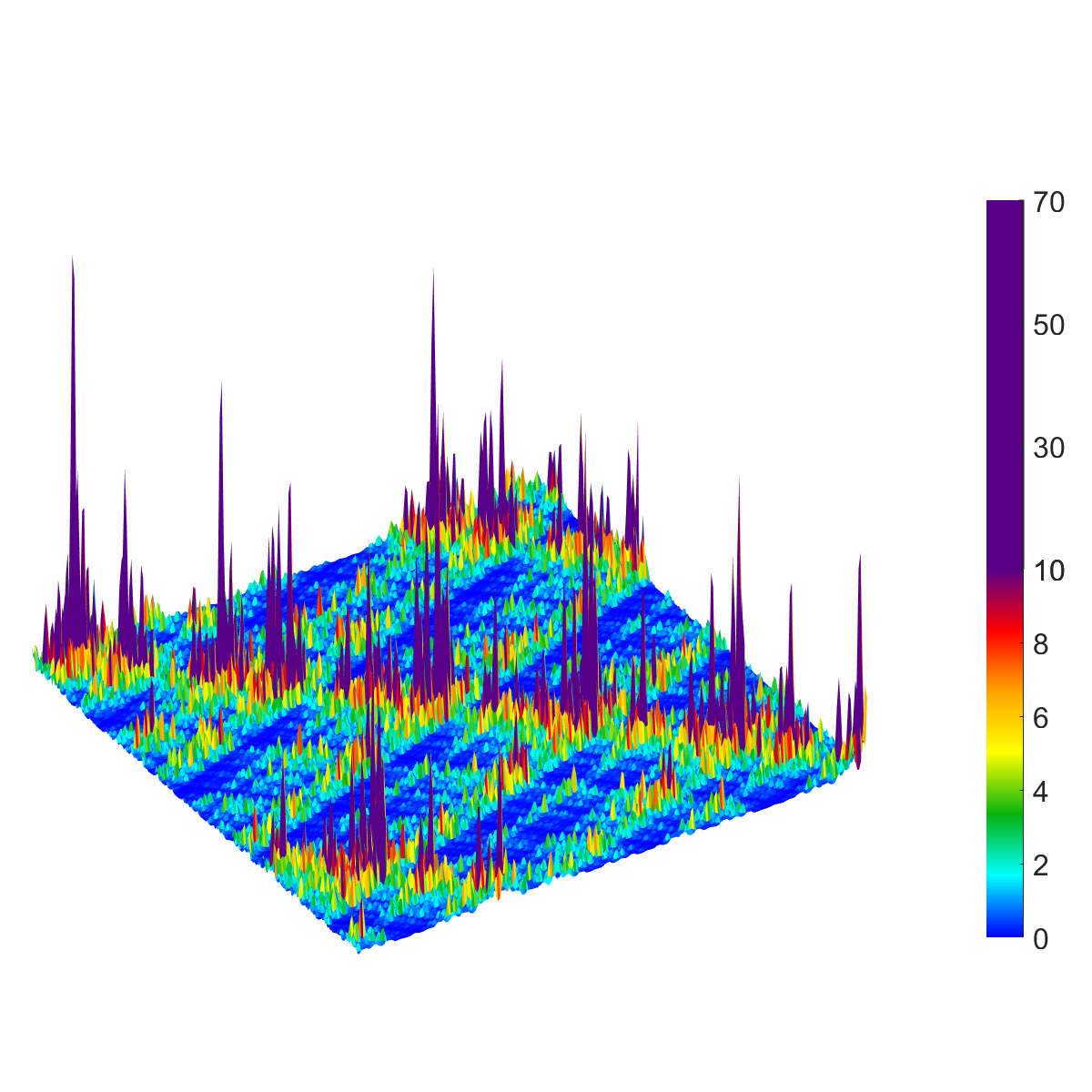
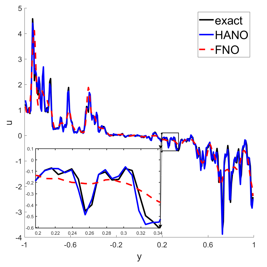
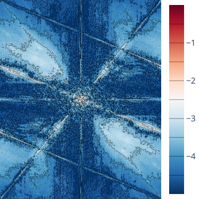
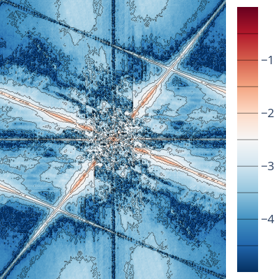
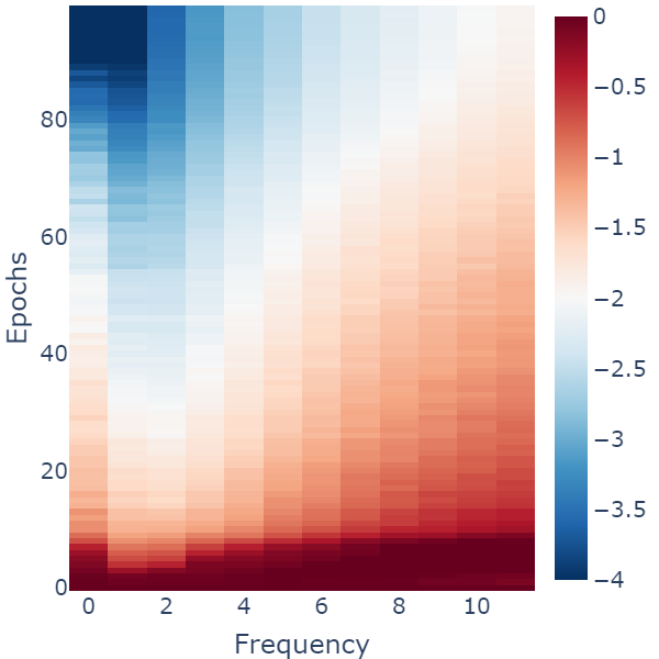
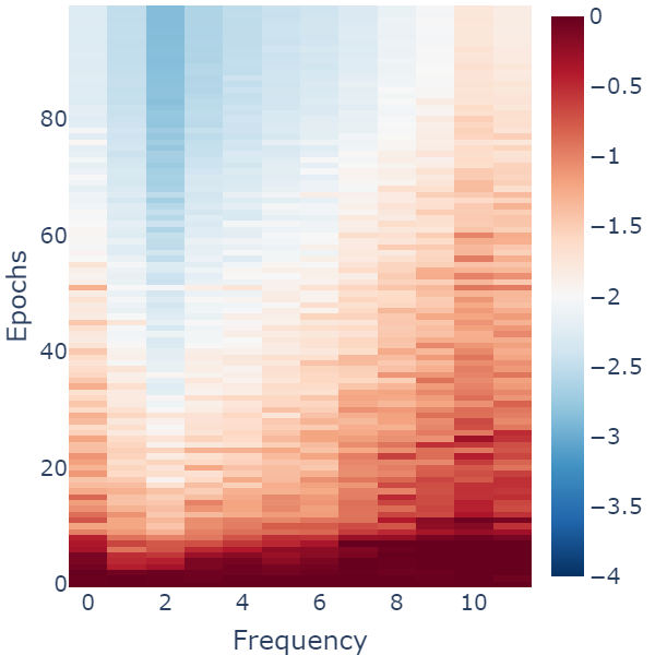
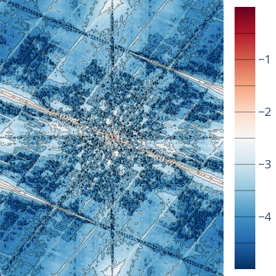
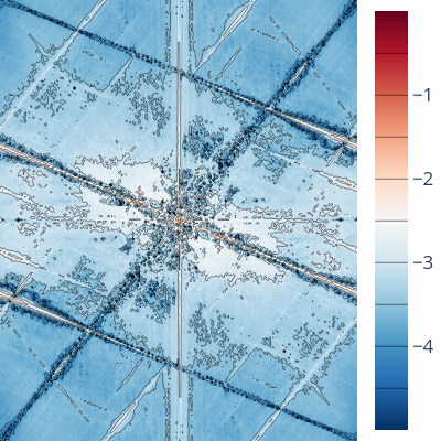
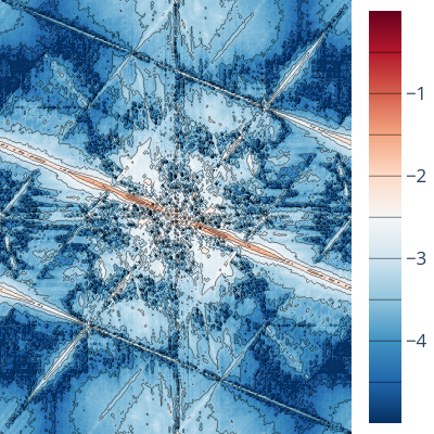
The spectral bias, also known as the frequency principle (Rahaman et al., 2019; Ronen et al., 2019; Xu et al., 2020), states that deep neural networks (DNNs) often struggle to learn high-frequency components of functions that vary at multiple scales. In this work, to our knowledge for the first time, we identify the issue of spectral bias for (multiscale) operator learning and thoroughly investigate it. As shown in Figure 1 and detailed in Section 4 and Appendix D, existing neural operators have difficulty learning high-frequency components of multiscale PDEs. Neural operators tend to fit low-frequency components faster than high-frequency ones, limiting their ability to accurately capture fine details. This motivates us to propose a new architecture for multiscale operator learning in this paper, using hierarchical attention and a tailored loss function to address this issue.

3 Methods

In this section, to address the spectral bias for multiscale operator learning, and motivated by the remarkable performance of attention-based models (Vaswani et al., 2017; Liu et al., 2021b) in computer vision and natural language processing tasks, as well as the effectiveness of hierarchical matrix approach (Hackbusch et al., 2002) for multiscale problems, we propose the Hierarchical Attention Neural Operator (HANO) model. We follow the setup in Li et al. (2021); Lu et al. (2021) to approximate the operator $\mathcal{S}:{\bm{a}}\mapsto{\bm{u}}:=\mathcal{S}({\bm{a}})$, with the input/parameter ${\bm{a}}\in\mathcal{A}$ drawn from a distribution $\mu$ and the corresponding output/solution ${\bm{u}}\in\mathcal{U}$, where $\mathcal{A}$ and $\mathcal{U}$ are infinite dimensional Banach spaces respectively. Our aim is to learn the operator $\mathcal{S}$ from a collection of finitely observed input-output pairs through a parametric map $\mathcal{N}:\mathcal{A}\times\Theta\rightarrow\mathcal{U}$ and a loss functional $\mathcal{L}:\mathcal{U}\times\mathcal{U}\rightarrow\mathbb{R}$.

Hierarchical discretization

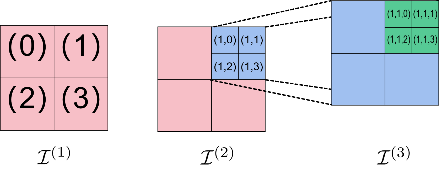
To develop hierarchical attention, we propose a hierarchical discretization of the spatial domain $D$, which can be extended to time-dependent PDEs by incorporating time-sliced data as feature channels. For a input feature map, for example, of resolution $8\times 8$ patches, we define $\mathcal{I}^{(3)}:=\{i=(i_{1},i_{2},i_{3})|i_{1},i_{2},i_{3}\in\{0,1,2,3\}\}$ as the finest level index set, in which each index $i$ corresponds to a patch token characterized by a feature vector ${\bm{f}}_{i}^{(3)}$ with $\mathcal{C}^{(3)}$ channels. For a token $i=(i_{1},i_{2},i_{3})$, its parent token $i^{(2)}=\left(i_{1},i_{2}\right)$ aggregates finer level tokens (e.g., $(1,1)$ is the parent of $(1,1,0),(1,1,1),(1,1,2),(1,1,3)$ in Figure 3). We postpone describing the aggregation scheme in the following paragraph. In general, we write $\mathcal{I}^{(r)}$ as the finest level token index set and $\mathcal{I}^{(m)}:=\{i^{(m)}:i\in\mathcal{I}^{(r)}\}$ as the index set of $m$-th level tokens. Note that the hierarchy is not restricted to quadtree setting.

Vanilla attention

We begin by recalling the vanilla attention mechanism, which operates on the finest level tokens ${\bm{f}}_{i}^{(r)}\in\mathbb{R}^{\mathcal{C}^{(r)}}$ indexed by $i\in\mathcal{I}^{(r)}$, and the token aggregation formula is given by

$$\textbf{atten}:{\bm{h}}_{i}^{(r)}=\sum_{j\in\mathcal{I}^{(r)}}\mathcal{G}({\bm{q}}_{i}^{(r)},{\bm{k}}_{j}^{(r)}){\bm{v}}_{j}^{(r)},$$ (1)

where $\bm{q}_{i}^{(r)}={\bm{W}}^{Q}{\bm{f}}_{i}^{(r)}$, $\bm{k}_{i}^{(r)}={\bm{W}}^{K}{\bm{f}}_{i}^{(r)}$, $\bm{v}_{i}^{(r)}={\bm{W}}^{V}{\bm{f}}_{i}^{(r)}$, and ${\bm{W}}^{Q}$, ${\bm{W}}^{K}$, ${\bm{W}}^{V}\in\mathbb{R}^{\mathcal{C}^{(r)}\times\mathcal{C}^{(r)}}$ are learnable matrices. Here, $\mathcal{G}$ represents the attention matrix via a softmax function.

Instead of computing equation 1 explicitly with $\mathcal{O}(N^{2})$ cost, we propose HANO, a hierarchically nested attention scheme with $\mathcal{O}(N)$ cost inspired by $\mathscr{H}^{2}$ matrices (Hackbusch, 2015). HANO scheme comprises four key operations: reduce, multilevel local attention, decompose, and mix.

Reduce operation

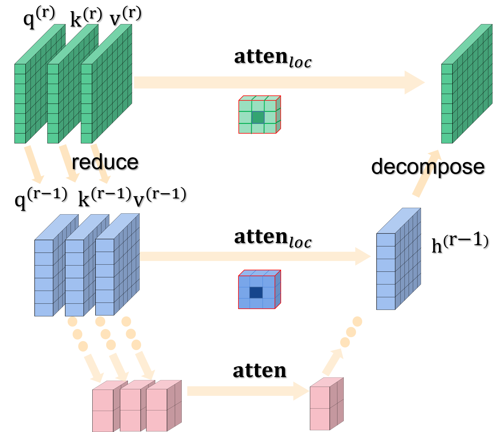
The reduce operation aggregates finer-level tokens into coarser-level tokens in the hierarchy. We denote $i^{(m,m+1)}$ as the set of indices of the $(m+1)$th level child tokens of the $m$th level token $i$, where $i\in\mathcal{I}^{(m)}$. In the quadtree case, $i^{(m,m+1)}=\{(i,0),(i,1),(i,2),(i,3)\}$, where $(i,j)$ is the concatenation of $i$ and $0\leq j\leq 3$. The reduce map can be defined as ${\bm{q}}_{i}^{(m)}=\mathcal{R}^{(m)}(\{{\bm{q}}_{j}^{(m+1)}\}_{j\in i^{(m,m+1)}})$, which maps the $(m+1)$th level tokens with indices in $i^{(m,m+1)}$ to the $m$th level token $i$. We implement $\mathcal{R}^{(m)}$ as a linear layer, namely, ${\bm{q}}_{i}^{(m)}={\bm{R}}_{0}^{(m)}{\bm{q}}_{(i,0)}^{(m+1)}+{\bm{R}}_{1}^{(m)}{\bm{q}}_{(i,1)}^{(m+1)}+{\bm{R}}_{2}^{(m)}{\bm{q}}_{(i,2)}^{(m+1)}+{\bm{R}}_{3}^{(m)}{\bm{q}}_{(i,3)}^{(m+1)}$, where ${\bm{R}}_{0}^{(m)},{\bm{R}}_{1}^{(m)},{\bm{R}}_{2}^{(m)},{\bm{R}}_{3}^{(m)}\in\mathbb{R}^{\mathcal{C}^{(m-1)}\times\mathcal{C}^{(m)}}$ are matrices. The reduce operation is applied to $\bm{q}_{i}^{(m)}$, $\bm{k}_{i}^{(m)}$, and $\bm{v}_{i}^{(m)}$ for any $i\in\mathcal{I}^{(m)}$, and $m=r-1,\cdots,1$. This step corresponds to the downwards arrow in Figure 3. The learnable reduce matrices ${\bm{R}}_{j}^{(m)}$ are a novel way to parameterize ${\bm{W}}^{Q},{\bm{W}}^{K},{\bm{W}}^{K}$ for coarse level query, key, value tokens. See Appendix B for details.

Remark 3.1.

Our nested token calculation approach differs from existing multiscale vision transformers (Liu et al., 2021b; Zhang et al., 2022), as we perform the reduce operation before attention aggregation, resulting in nested ${\bm{q}},{\bm{k}},{\bm{v}}$ tokens. Additionally, our approach differs from UNet (Ronneberger et al., 2015), which utilizes maxpooling for the reduce operation. Please refer to Table 1 for the comparison of performances.

Figure 2: Hierarchical discretization and index tree. The 2D unit square is discretized hierarchically into three levels with corresponding index sets $\mathcal{I}^{(1)},\mathcal{I}^{(2)}$, and $\mathcal{I}^{(3)}$. To illustrate, $(1)^{(1,2)}$ represents the second level child nodes of node $(1)$ and is defined as $(1)^{(1,2)}=\{(1,0),(1,1),(1,2),(1,3)\}$.

Figure 3: Hierarchically nested attention.

Multilevel local attention

Instead of using global attention aggregation as in equation 1, we utilize a local aggregation formula inspired by the $\mathcal{H}$ matrix approximation. This approximation suggests that global interactions can be decomposed into local interactions at different scales (levels of tokens) with minimal loss of expressivity. The local aggregation at the $m$-th level $\textbf{atten}^{(m)}_{\textrm{loc}}$ is written using the nested $\bm{q}_{i}^{(m)},\bm{k}_{j}^{(m)},\bm{v}_{j}^{(m)}$ for $m=r,\ldots,1$ as follows: for $i\in\mathcal{I}^{(m)},$

$$\textbf{atten}^{(m)}_{\textrm{loc}}:{{\bm{h}}}_{i}^{(m)}=\sum_{j\in\mathcal{N}^{(m)}(i)}\mathcal{G}(\bm{q}_{i}^{(m)}\cdot\bm{k}_{j}^{(m)})\bm{v}_{j}^{(m)}$$ (2)

Here, $\mathcal{N}^{(m)}(i)$ is the set of $m$-th level neighbors of $i\in\mathcal{I}^{(m)}$. We employ window attention (Liu et al., 2021b) for attention within the neighbor set $\mathcal{N}^{(m)}(i)$, where the interaction range of local attention is determined by the window size.

Decompose and mix operations

We propose a decompose operation that reverses the reduce operation from level $1$ to level $r-1$. The decompose operator $\mathcal{D}^{(m)}:{\bm{h}}_{i}^{(m)}\mapsto\{\tilde{{\bm{h}}}_{j}^{(m+1)}\}_{j\in i^{(m,m+1)}}$, maps the $m$-th level feature ${{\bm{h}}}_{i}^{(m)}$ with index $i$ and $1\leq m\leq r-1$ to $(m+1)$-th level tokens associated to its child set $i^{(m,m+1)}$. $\tilde{{\bm{h}}}_{i}^{(m+1)}$ is further aggregated to ${{\bm{h}}}_{i}^{(m+1)}$ in the mix operation such that ${\bm{h}}_{i}^{(m+1)}+=\tilde{{\bm{h}}}_{i}^{(m+1)}$ for $i\in\mathcal{I}^{(m+1)}$. In the current implementation, we use a simple linear layer such that $\tilde{{\bm{h}}}_{(i,s)}^{(m+1)}={\bm{D}}_{s}^{(m),T}{\bm{h}}_{i}^{(m)}$, for $s=0,1,2,3$, with parameter matrices ${\bm{D}}_{s}^{(m)}\in\mathbb{R}^{\mathcal{C}^{(m)}\times\mathcal{C}^{(m+1)}}$.

Remark 3.2.

In our current implementation, the operators $\mathcal{R}^{(m)}$ and $\mathcal{D}^{(m)}$ only consist of linear layers. In general, these operators may contain nonlinear activation functions. The nested learnable matrices ${\bm{R}}^{(m)}$ and ${\bm{D}}^{(m)}$ induce channel mixing and a structured parameterization to the ${\bm{W}}^{Q},{\bm{W}}^{V},{\bm{W}}^{K}$ matrices for coarse level tokens, resulting in possibly low-rank approximations of the attention matrix. Appendix B provides the equivalent matrix form of $\mathcal{R}^{(m)}$ and $\mathcal{D}^{(m)}$ from fine to coarse levels.

We summarize the hierarchically nested attention algorithm in the following.

Algorithm 1 Hierarchically Nested Attention

  Input: $\mathcal{I}^{(r)}$, ${\bm{f}}_{i}^{(r)}$ for $i\in\mathcal{I}^{(r)}$.STEP 0: Compute $\bm{q}_{i}^{(r)}$, $\bm{k}_{i}^{(r)}$, $\bm{v}_{i}^{(r)}$ for $i\in\mathcal{I}^{(r)}$. STEP 1: For $m=r-1,\cdots,1$, Do the reduce operations $\bm{q}_{i}^{(m)}=\mathcal{R}^{(m)}(\{\bm{q}_{j}^{(m+1)}\}_{j\in i^{(m,m+1)}})$ and also for $\bm{k}_{i}^{(m)}$ and $\bm{v}_{i}^{(m)}$, for any $i\in\mathcal{I}^{(m)}$. STEP 2: For $m=r,\cdots,1$, Do the local aggregation by equation 2 to compute ${{\bm{h}}}_{i}^{(m)},m=1,...,r,$ for any $i\in\mathcal{I}^{(m)}$.STEP 3: For $m=1,\cdots,r-1$, Do the decompose operations $\{\tilde{{\bm{h}}}_{j}^{(m+1)}\}_{j\in i^{(m,m+1)}}=\mathcal{D}^{(m)}({\bm{h}}_{i}^{(m)})$, for any $i\in\mathcal{I}^{(m)}$; then ${\bm{h}}_{i}^{(m+1)}+=\tilde{{\bm{h}}}_{i}^{(m+1)}$, for any $i\in\mathcal{I}^{(m+1)}$.Output: ${\bm{h}}_{i}^{(r)}$ for any $i\in\mathcal{I}^{(r)}$.

Proposition 3.3 (Complexity of Algorithm 1).

The reduce operation, multilevel local attention, and decomposition/mix operations together form a V-cycle for updating tokens, as illustrated in Figure 3. The cost of one V-cycle is $O(N)$ if $\mathcal{I}$ is a quadtree, as implemented in the paper. Please refer to Appendix C for the proof of this complexity.

Comparison with Existing Multiscale Transformers

In multiscale vision transformers like Liu et al. (2021b); Zhang et al. (2022), attentions are performed at each level separately, resulting in no multilevel attention-based aggregation. This may lead to the loss of fine-scale information in the coarsening process, which is not ideal for learning multiscale operators where fine-scale features are crucial. To address this issue, we develop the following components in the HANO approach: (1) Attention-based local aggregations at each level, followed by summation of features from all levels to form the updated fine-scale features; (2) The reduce/local aggregation/decompose/mix operations, inspired by the $\mathcal{H}^{2}$ hierarchical matrix method, enable the recovery of fine details with a linear cost; (3) Nested computation of features at all levels, with simultaneous parameterization of the learnable matrices $W_{Q},W_{K},W_{V}$ in a nested manner. Those components highlight the novelty of our method.

Remark 3.4.

Our attention matrix has a global interaction range but features low-rank off-diagonal blocks at each level, as shown in Appendix B. Note that the attention matrix itself is not necessarily low-rank, distinguishing it from efficient attention models using kernel tricks or low-rank projections(Choromanski et al., 2020; Wang et al., 2020b; Peng et al., 2021; Nguyen et al., 2021; Cao, 2021; Xiong et al., 2021).

4 Experiments

We demonstrate that HANO achieves superior performance compared to other state-of-the-art neural operators and transformers for learning multiscale operators in two dimensions. We evaluate its performance on solving multiscale elliptic PDEs, a benchmark task for operator learning. HANO demonstrates higher accuracy and robustness for coefficients with different degrees of roughness/multiscale features. HANO also provides lower generalization error for out-of-distribution input parameters. Furthermore, we apply HANO to the Navier-Stokes equations, a benchmark problem with nonlinearity, time dependence, and high Reynolds number. We also include a benchmark for the Helmholtz equation in Appendix F.2.

4.1 Setup

We consider pairs of functions ${({\bm{a}}_{j},{\bm{u}}_{j})}_{j=1}^{N}$, where ${\bm{a}}_{j}$ is drawn from a probability measure $\mu$ and ${\bm{u}}_{j}=\mathcal{S}({\bm{a}}_{j})$. To train and test our model, we evaluate ${\bm{a}}_{j}$ and ${\bm{u}}_{j}$ pointwisely in the uniform 2D grid $\mathsf{G}^{2}$. We generate the hierarchical index tree $\mathcal{I}$ using the quadtree representation of nodes with depth $r$, where the finest level objects are pixels or patches aggregated by pixels. Further details can be found in Appendix E.

Architecture

We implement HANO using the standard transformer architecture Dosovitskiy et al. (2020), with emphasis on the attention mechanim. The input ${\bm{a}}$ is first embedded into $n\times n$ tokens represented as a tensor of size $n\times n\times\mathcal{C}^{(r)}$ using patch embedding, for a dataset with resolution $n_{f}\times n_{f}$, such as in the multiscale elliptic equation benchmark. These tokens are then processed by a multi-level hierarchically nested attention, as described in Section 3, resulting in hidden features ${{\bm{h}}_{i}^{(r)},i\in\mathcal{I}^{(r)}}$. Finally, a decoder maps the hidden features to the solution ${\bm{u}}$. Different decoders can be employed depending on prior knowledge of the PDE model. For example, Lu et al. (2021) uses a simple feedforward neural network (FFN) to learn a basis set, Bhattacharya et al. (2021) employs a data-driven SVD-based decoder, and in our work, we use spectral convolution layers from Li et al. (2021). We refer readers to Appendix E for more implementation details.

Empirical $H^{1}$ Loss Function

Loss functions are crucial for efficient training and robust generalization of neural network models. For multiscale problems, we adopt the $H^{1}$ loss function instead of the conventional $L^{2}$ loss, which places greater emphasis on high-frequency components. We define the empirical $L^{2}$ loss function as $\mathcal{L}^{L}(\left\{(\bm{a}_{j},\bm{u}_{j})\right\}_{j=1}^{N};\theta):=\frac{1}{N}\sum_{i=1}^{N}\|\bm{u}_{j}-\mathcal{N}(\bm{a}_{j};\theta)\|_{l^{2}}/\|\bm{u}_{j}\|_{l^{2}}$, where $|\cdot|_{l^{2}}$ is the canonical $l^{2}$ vector norm. The normalized discrete Fourier transform (DFT) coefficients of $f$ are given by $\mathcal{F}(f)(\xi):=\frac{1}{\sqrt{n}}\sum_{x\in\mathsf{G}^{2}}f(x)e^{-2i\pi x\cdot\xi}$ for any $\xi\in\mathbb{Z}_{n}^{2}:=\left\{\xi\in\mathbb{Z}^{2}\mid-n/2+1\leqslant\xi_{j}\leqslant n/2,j=1,2\right\}$. The empirical $H^{1}$ loss function is thus given by, $\mathcal{L}^{H}(\left\{(\bm{a}_{j},\bm{u}_{j})\right\}_{j=1}^{N};\theta):=\frac{1}{N}\sum_{i}\|{\bm{u}}_{j}-\mathcal{N}(\bm{a}_{j};\theta)\|_{h}/\|\bm{u}_{j}\|_{h},$ where $\|{\bm{u}}\|_{h}:=\sqrt{\sum_{\xi\in\mathbb{Z}_{n}^{2}}|\xi|^{2}(\mathcal{F}({\bm{u}})(\xi))^{2}}$. $\mathcal{L}^{H}$ can be viewed as a weighted $\mathcal{L}^{L}$ loss using $|\xi|^{2}$ weights to capture high-frequency components. We use the frequency space representation of the discrete $H^{1}$ norm here, but the discrete $H^{1}$ norm in real space can also be employed.

Remark 4.1.

The $H^{1}$ loss here is defined on the target solution space and measures the difference between the predicted and true solutions. In contrast to Yu et al. (2022) where the loss function is defined with respect to the input variable, our loss function is defined with respect to the spatial variable.

4.2 Multiscale Elliptic Equations

(a) coefficient

(b) reference

(c) HANO prediction

(d) abs. error of HANO

(e) abs. error of FNO2D

Figure 4: Top: (a) smooth coefficient in Li et al. (2021), with $a_{\max}=12,$ $a_{\min}=3$, $c=9$, (b), reference solution, (c) HANO solution, (d) HANO, absolute (abs.) error, (e) FNO2D, abs. error; Bottom: (a) rough coefficients with $a_{\max}=12,$ $a_{\min}=2$, $c=20$, (b) reference solution, (c) HANO solution, (d) HANO, abs. error, (e) FNO2D, abs. error, the maximal error of FNO2D is around $900\mu=9\mathrm{e}{-4}$.

Table 1: The baseline methods are implemented with their official implementation if publicly available. Performance are measured with relative $L^{2}$ errors ($\times 10^{-2}$) and relative $H^{1}$ errors ($\times 10^{-2}$). For the Darcy rough case, we run each experiment 3 times to calculate the mean and the standard deviation (after $\pm$) of relative $L^{2}$ and relative $H^{1}$ errors. All experiments use a fixed train-val-test split setup, see E.2 for details.

			Darcy smooth		Darcy rough		Multiscale
	Model	Runtime (s)	$L^{2}$	$H^{1}$	$L^{2}$	$H^{1}$	$L^{2}$	$H^{1}$
	FNO2D	7.278	$0.706$	$3.131$	$1.782$ $\pm 0.021$	$9.318$ $\pm 0.088$	$1.949$	$14.535$
	FNO2D $H^{1}$	$7.391$	$0.684$	$2.583$	$1.613$ $\pm 0.010$	$7.516$ $\pm 0.049$	$1.800$	$9.619$
	FNO2D-48	$8.062$	$0.619$	$2.620$	$1.220$ $\pm 0.018$	$5.138$ $\pm 0.093$	$1.565$	$11.093$
	FNO2D-96	$10.969$	$0.575$	$2.437$	$1.216$ $\pm 0.024$	$5.140$ $\pm 0.281$	$1.518$	$10.106$
	UNet	9.127	$2.169$	$4.885$	$3.591$ $\pm 0.127$	$6.479$ $\pm 0.311$	$1.425$	$5.012$
	U-NO	$11.259$	$0.678$	$2.580$	$1.185$ $\pm 0.005$	$5.695$ $\pm 0.005$	$1.350$	$8.577$
	U-NO $H^{1}$	$11.428$	$0.492$	$1.276$	$1.023$ $\pm 0.013$	$3.784$ $\pm 0.016$	$1.187$	$5.380$
	MWT	$19.715$	—	—	$1.138$ $\pm 0.010$	$4.107$ $\pm 0.008$	$1.021$	$7.245$
	GT	$38.219$	$0.945$	$3.365$	$1.790$ $\pm 0.012$	$6.269$ $\pm 0.418$	$1.052$	$8.207$
	SWIN	$41.417$	—	—	$1.622$ $\pm 0.047$	$6.796$ $\pm 0.359$	$1.489$	$13.385$
	HANO-s	$14.851$	$0.330$	$0.899$	$0.737$$\pm 0.006$	$1.977$$\pm 0.023$	$0.805$	$3.121$
	HANO-l	$33.375$	$0.291$	$0.815$	$0.571$$\pm 0.010$	$1.371$$\pm 0.011$	$0.579$	$1.985$
— MWT (Gupta et al., 2021) only supports resolution with powers of two.

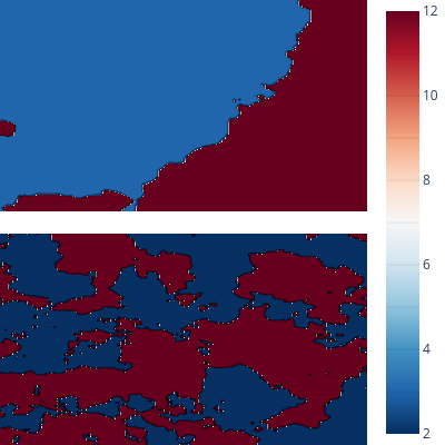
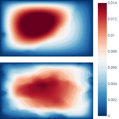
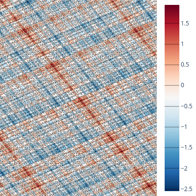
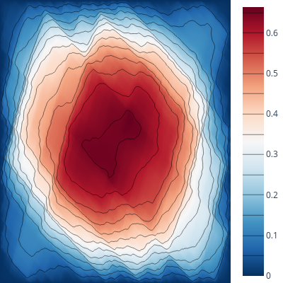
We apply the HANO model to learn the mapping from coefficient functions to solution operators for multiscale elliptic equations. We use the two-phase coefficient model proposed in Li et al. (2021) and also studied in Gupta et al. (2021); Cao (2021). Unlike previous works where the coefficient functions are relatively smooth and the solutions are also smooth (which we call "Darcy smooth"), we adjust the parameters controlling the smoothness and contrast of the coefficients to generate solutions with more roughness (which we call "Darcy rough"). See Figure 4 for an example. Details on how we generate the data are provided in Appendix A.1.2. We also include experiments for multiscale trigonometric coefficients with higher contrast; see Appendix A.1.1 for details. Results for three benchmarks are summarized in Table 1. Additionally, we compare HANO with two conventional numerical methods in Appendix F.3 and show that HANO achieves comparable accuracy with significantly better efficiency.

Spectral Bias in Operator Learning

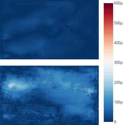
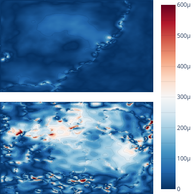
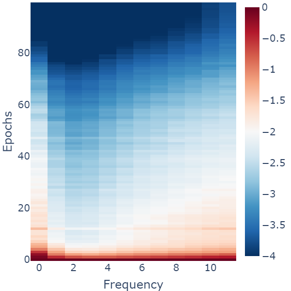
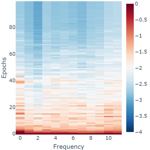
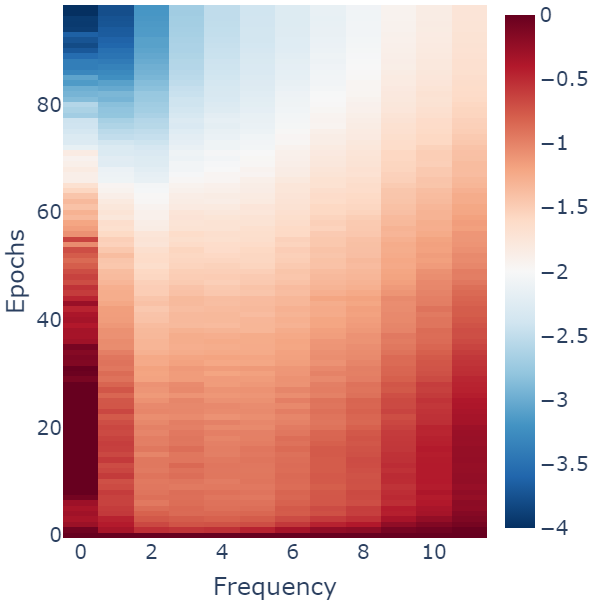
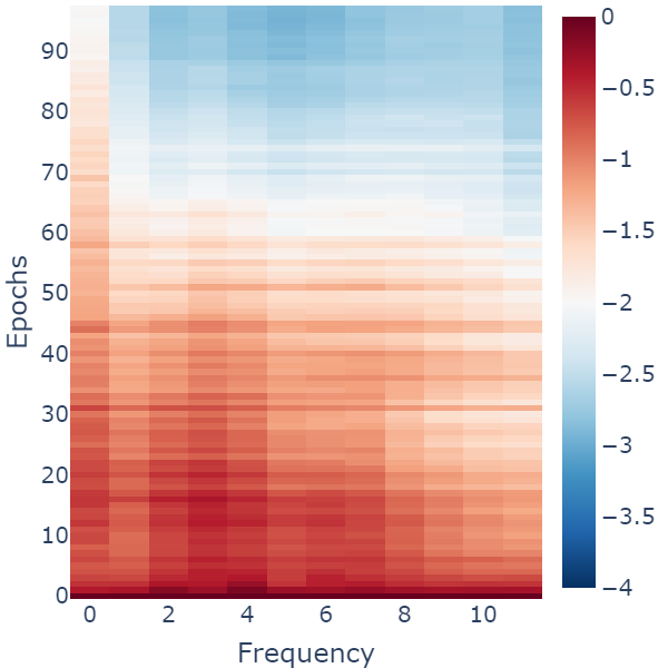
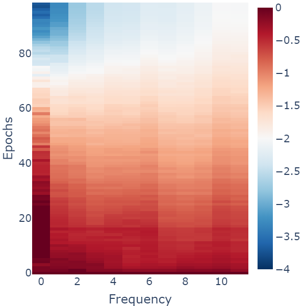
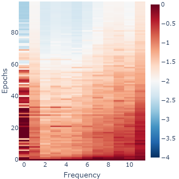
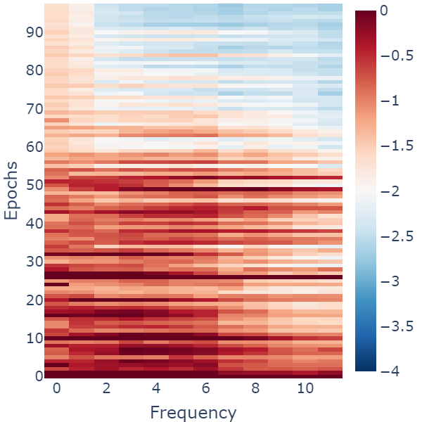
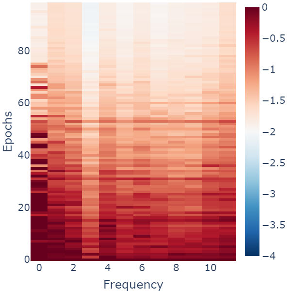
We compare HANO and FNO in terms of prediction error dynamics across frequencies from epoch 0 to epoch 100 (end) in Figure 5 (other models have similar patterns to FNO, see Appendix D for a comprehensive comparison and experiment setup). The subfigures (c,d) in Figure 5 and also Figure 10 suggest that existing methods can learn low frequencies quickly but struggle with high frequencies. At the end of the training, plenty of high frequency components are still not well resolved as shown in Figure 1(b,c,d) and Figure 9. We call this phenomenon spectral bias in operator learning. On the contrary, HANO’s error decays faster for higher frequencies and more uniformly overall. It also achieves lower testing errors. The hierarchical nested attention allows the model to capture fine-scale variations according to the $\mathcal{H}$ matrix theory (Hackbusch et al., 2002). With the $H^{1}$ loss function, spectral bias is further mitigated; thus, HANO outperforms existing methods. This is consistent with Figure1, where HANO shows superiority in predicting fine-scale features.

(a)

(b)

(c)

(d)

Figure 5: (a) shows the training error dynamics, with x-axis for the first 12 dominating frequencies (low frequency $\rightarrow$ high frequency from left to right), y-axis for the number of training epoch, and colorbar for normalized $L^{2}$ error (w.r.t the error at epoch $0$) in $\log_{10}$ scale. (b) shows the corresponding testing errors. (c)(d) display the training and testing error dynamics of FNO.

Comparison with Existing Methods

We perform comprehensive comparison with existing methods: (1) It is natural to hypothesize that more frequency modes in FNO may help reduce the spectral bias, and a way to incrementally add more modes during training is proposed in Zhao et al. (2022). We evaluate the impact of increasing frequency modes by including FNO2D-48 and FNO2D-96, with 48 and 96 modes respectively, adapted from the default FNO2D model with 12 modes. (2) UNet (Ronneberger et al., 2015) and U-NO, a U-shaped neural operator (Rahman et al., 2022); (3) multiwavelet neural operator (MWT) (Gupta et al., 2021); (4) Galerkin transformer (GT) (Cao, 2021); (5) SWIN Liu et al. (2021b) as a representative multiscale vision transformer, where we replaced the hierarchical attention module of HANO by the SWIN code. In addition, we trained FNO2D (FNO2D $H^{1}$), U-NO (U-NO $H^{1}$) with $H^{1}$ loss to evaluate the effect of $H^{1}$ loss. We also trained HANO-s and HANO-l with feature dimension $24$ and $64$, respectively, to evaluate the impact of feature dimension. We conclude that HANO significantly outperforms other neural operators for all three tasks, even for the smaller model HANO-s. $H^{1}$ loss is effective for general architectures, e.g., comparing FNO2D, U-NO, with their $H^{1}$ loss trained variants FNO2D $H^{1}$, and U-NO $H^{1}$. HANO-s can already achieve significant improvement with reduced runtime. As shown in Figure 4, from Darcy smooth to Darcy rough to multiscale trignometric, as the presence of high-frequency components increases, and the superiority of HANO over other methods becomes more evident.

Out of Distribution Test

In the OOD (out of distribution) test in Table 2, we trained the model using rough coefficients with $a_{\max}=12,$ $a_{\min}=2$, and $c=20$, and tested the model using coefficients with $a_{\max}=12,$ $a_{\min}=4$, and $c=18$. Namely, the testing samples were generated with different contrast and smoothness compared with the training samples. See Appendix A.1.2 for details. HANO trained with $H^{1}$ loss also generalizes better on out of distribution samples. We compare HANO with other models in Table 2. The models are trained with the same setup. HANO outperforms other models by order of magnitude. See also Appendix F.1 for the training dynamics.

	FNO2D	FNO2D $H^{1}$	MWT	HANO
$n=256$	$20.27$	11.49	21.901	3.182

Table 2: Rel. $L^{2}$ err. ($\times 10^{-2}$) for OOD data.

4.3 Navier-Stokes Equation

We consider the 2D Navier-Stokes equation in vorticity form on the unit torus $\mathsf{T}$ (see A.2 for details), as benchmarked in Li et al. (2021). The vorticity is $\omega(x,t)$, for $x\in\mathsf{T}$ and $t\in[0,T]$. We learn the operator $\mathcal{S}:w(\cdot,0\leq t\leq 9)\rightarrow w(\cdot,10\leq t\leq T)$, mapping the vorticity up to time 9 to the vorticity up to some later time $T$. We experiment with viscosities $\nu=1\mathrm{e}-3,1\mathrm{e}-4,1\mathrm{e}-5$, and decrease the final time $T$ accordingly as the dynamics becomes more turbulent with increasing Reynolds number.

Time dependent neural operator

Following the setup in Li et al. (2021), we fix the resolution as $64\times 64$ for both training and testing. The ten time-slices of solutions $w(\cdot,t)$ at $t=0,...,9$ are taken as the input data to the neural operator $\mathcal{N}$ which maps the solutions at the previous 10 timesteps to the next time step (2D functions to 2D functions). This procedure, often referred to as the rolled-out prediction, can be repeated recurrently until the final time $T$. We list the results of HANO, FNO-3D (convolution in space-time), FNO-2D, U-Net (Ronneberger et al., 2015), TF-NetWang et al. (2020a), ResNetHe et al. (2016) and DilResNetStachenfeld et al. (2022) in Table 3, and HANO clearly achieves the best performance.

		$T=50$	$T=30$	$T=30$	$T=20$
Model	#Parameters	$\nu=1\mathrm{e}-3$	$\nu=1\mathrm{e}-4$	$\nu=1\mathrm{e}-4$	$\nu=1\mathrm{e}-5$
		$N=1000$	$N=1000$	$N=10000$	$N=1000$
FNO-3D	$6,558,537$	$0.0086$	$0.1918$	$0.0820$	$0.1893$
FNO-2D	$926,517$	$0.0128$	$0.1559$	$0.0834$	$0.1556$
U-Net	$24,950,491$	$0.0245$	$0.2051$	$0.1190$	$0.1982$
TF-Net	$7,451,724$	$0.0225$	$0.2253$	$0.1168$	$0.2268$
ResNet	$266,641$	$0.0701$	$0.2871$	$0.2311$	$0.2753$
DilResNet	$586,753$	0.0315	0.2561	0.2081	0.2315
HANO-l	$10,707,204$	$\mathbf{0.0050}$	$\mathbf{0.0517}$	$\mathbf{0.0194}$	$\mathbf{0.0690}$
HANO-s	$1,083,944$	$0.0098$	$0.1151$	$0.0618$	$0.1220$

Table 3: Benchmark for the Navier-Stokes equation. $64\times 64$ resolution is used for both training and testing, with $500$ epochs for all models. $N$ is the training sample size, either $N=1000$ or $N=10000$. The number of testing samples is 100 or 1000, respectively.

5 Conclusion

In this work, we investigated the spectral bias phenomenon commonly observed in multiscale operator learning. To our best knowledge, we conducted the first in-depth study of this issue. We proposed HANO, a hierarchical attention-based model to mitigate spectral bias. HANO employs a fine-coarse-fine V-cycle update and an empirical $H^{1}$ loss to recover fine-scale features in the multiscale solutions. Our experiments show that HANO outperforms existing neural operators on multiscale benchmarks in terms of accuracy and robustness.

Limitation and outlook (1) HANO’s current implementation requires a regular grid, and extending it to data clouds and graph neural networks could offer new opportunities to exploit its hierarchical representation. (2) The current attention-based operator in HANO can achieve discretization invariance using simple interpolation (Kovachki et al., 2023), see also Appendix F.4. However, either simple interpolation or Fourier interpolation (used by FNO) may suffer from aliasing errors in the frequency domain, as indicated by our experiments and recent analysis (Kovachki et al., 2021; Lanthaler et al., 2022). Better balance between discretization invariance and model accuracy may be achieved with proper operator-adaptive sampling and interpolation techniques.

Appendix A Multiscale PDEs

In this section, we introduce some mathematical and numerical concepts related to multiscale PDEs.

A.1 Multiscale Elliptic PDEs

The second order elliptic equation with divergence form writes

$$\left\{\begin{aligned} -\nabla\cdot(a(x)\nabla u(x))&=f(x)&&x\in D\\ u(x)&=0&&x\in\partial D\end{aligned}\right.$$ (3)

where the coefficient $0<a_{\min}\leq a(x)\leq a_{\max},\forall x\in D$, and the forcing term $f\in H^{-1}(D;\mathbb{R})$. The coefficient to solution map is $\mathcal{S}:L^{\infty}(D;\mathbb{R}_{+})\rightarrow H_{0}^{1}(D;\mathbb{R})$, such that $u=\mathcal{S}(a)$. The setup of rough or multiscale coefficient $a(x)$ allows fast oscillation (e.g. $a(x)=a(x/\varepsilon)$ with $\varepsilon\ll 1$), high contrast ratio with $a_{\max}/a_{\min}\gg 1$, and even a continuum of non-separable scales.

A.1.1 Multiscale trigonometric coefficient

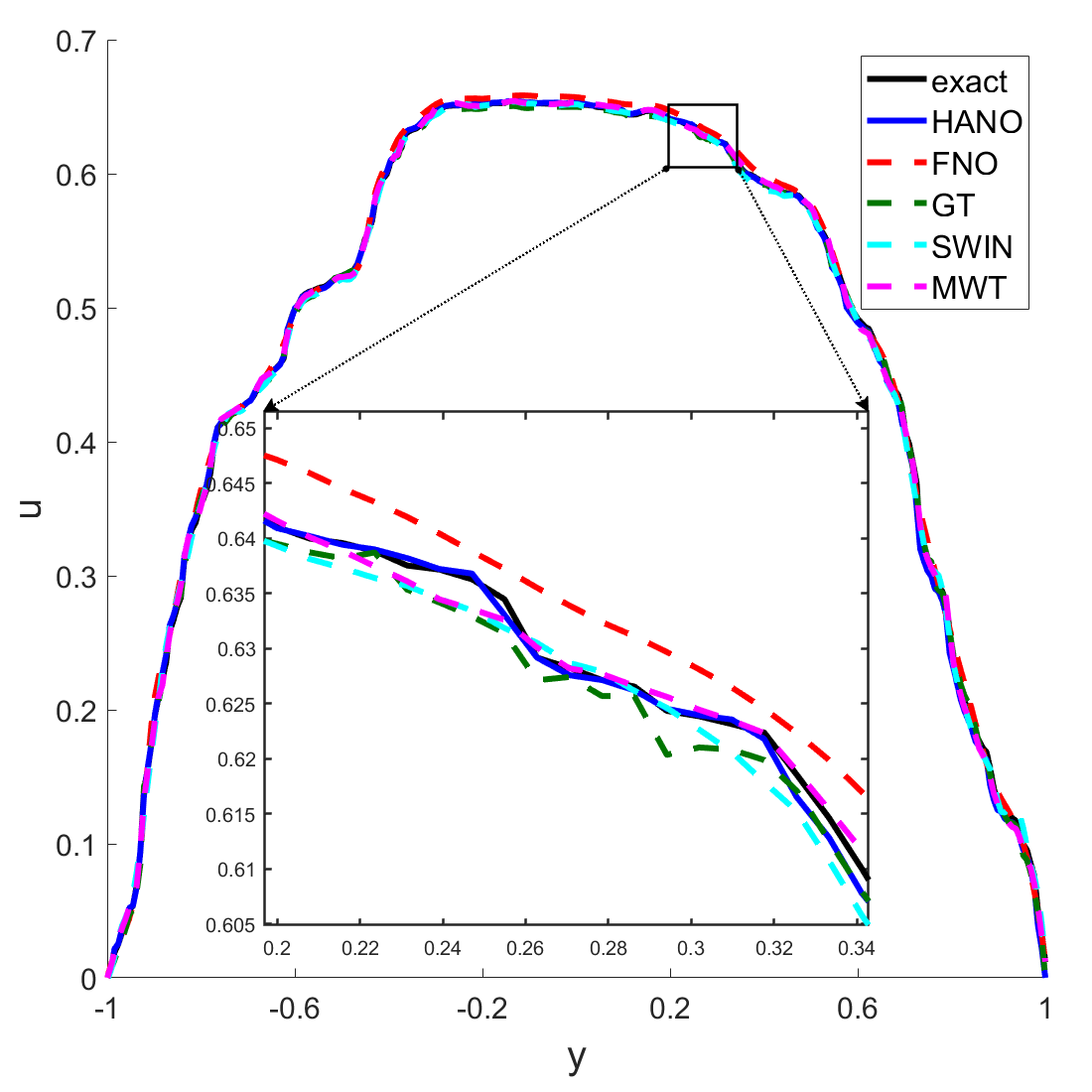
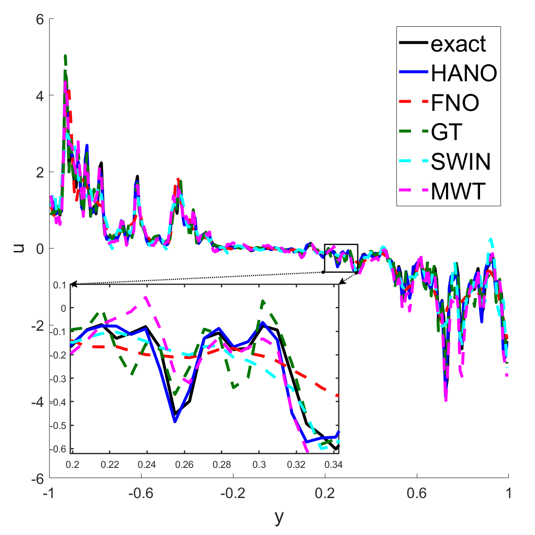
We consider equation 3 with multiscale trigonometric coefficient adapted from Owhadi (2017), which is one of the multiscale elliptic equation benchmarks in Section 4.2. The domain $D$ is $[-1,1]^{2}$, and the coefficient $a(x)$ is defined as $a(x)=\prod\limits_{k=1}^{6}(1+\frac{1}{2}\cos(a_{k}\pi(x_{1}+x_{2})))(1+\frac{1}{2}\sin(a_{k}\pi(x_{2}-3x_{1})))$, where $a_{k}$ is uniformly distributed between $2^{k-1}$ and $1.5\times 2^{k-1}$, and the forcing term is fixed as $f(x)\equiv 1$. The reference solutions are obtained using $\mathcal{P}_{1}$ FEM on a $1023\times 1023$ grid. Datasets of lower resolution are created by downsampling the higher resolution dataset using linear interpolation. The experiment results for the multiscale trigonometric case with different resolutions are shown in Table 1. HANO obtains the best relative $L^{2}$ error compared to other neural operators. See Figures 1 and 8 for illustrations of the coefficient and comparison of the solutions/derivatives at the slice $x=0$.

A.1.2 Two-Phase Coefficient

The two-phase coefficients and solutions (referred to as Darcy smooth and Darcy rough) in Section 4.2 are generated according to https://github.com/zongyi-li/fourier_neural_operator/tree/master/data_generation, and used as an operator learning benchmark in Li et al. (2021); Gupta et al. (2021); Cao (2021). The coefficients $a(x)$ are generated according to $a\sim\mu:=\psi_{\#}\mathcal{N}\left(0,(-\Delta+cI)^{-2}\right)$ with zero Neumann boundary conditions on the Laplacian. The mapping $\psi:\mathbb{R}\rightarrow\mathbb{R}$ takes the value $a_{\max}$ on the positive part of the real line and $a_{\min}$ on the negative part. The push-forward is defined in a pointwise manner. The forcing term is fixed as $f(x)\equiv 1$. Solutions $u$ are obtained by using a second-order finite difference scheme on a suitable grid. The parameters $a_{\max}$ and $a_{\min}$ can control the contrast of the coefficient. The parameter $c$ controls the roughness (oscillation) of the coefficient; a larger $c$ results in a coefficient with rougher two-phase interfaces, as shown in Figure 4.

A.2 Navier Stokes Equation

The Navier Stokes equation in vorticity form writes

$$\partial_{t}w(x,t)+u(x,t)\cdot\nabla w(x,t) =\nu\Delta w(x,t)+f(x),$$

$$\nabla\cdot u(x,t) =0,$$

$$w(x,0) =w_{0}(x),$$

where $u$ is the velocity, $w$ is the vorticity field, $w_{0}$ is the initial vorticity field, $\nu$ is the viscosity, $f$ is a forcing term, and $\mathrm{Re}$ is the Reynolds number, defined as $\mathrm{Re}:=\frac{\rho uL}{\nu}$ with the density $\rho$ ($=1$ here), the fluid velocity $u$, and the length scale of the fluid $L$ ($=1$ here). The Reynolds number is a dimensionless parameter and is inversely proportional to the viscosity $\nu$. When Re is greater than 2,900, the flow becomes turbulent.

A.3 Numerical Homogenization, Multilevel/Multigrid Methods, and Operator Learning

Let $\varepsilon$ be the smallest scale of the multiscale problem and $H$ be a coarse computational scale determined by the available computational power and the desired precision, such that $\varepsilon\ll H\ll 1$. The goal of numerical homogenization is to construct a finite-dimensional approximation space $V_{H}$ and to seek an approximate solution $u_{H}\in V_{H}$, such that, the accuracy estimate $\|u-u_{H}\|\leq CH^{\alpha}$ holds for optimal choices of the norm $\|\cdot\|$ and the exponent $\alpha$, and optimal computational cost holds with $V_{H}$ constructed via pre-computed subproblems which are localized, independent and do not depend on the RHS and boundary condition of the problem. In recent two decades, great progress has been made in this area (Hou et al., 1999; Målqvist & Peterseim, 2014; Owhadi & Zhang, 2007), approximation spaces with optimal accuracy (in the sense of Kolmogorov $N$-width (Berlyand & Owhadi, 2010)) and cost can be constructed for elliptic equations with fixed rough coefficients.

Multilevel/multigrid methods can be seen as the multilevel generalization of numerical homogenization methods for multiscale PDEs. Numerical homogenization can provide coarse spaces with optimal approximation and localization properties. Recently, operator-adapted wavelets (gamblets) have been developed (Owhadi, 2017; Xie et al., 2019). Gamblets enjoy three properties that are ideal for the construction of efficient direct methods: scale orthogonality, well-conditioned multi-resolution decomposition, and localization. Gamblets have been generalized to efficiently solve the Navier-Stokes equation (Budninskiy et al., 2019) and the Helmholtz equation (Hauck & Peterseim, 2022).

For multiscale partial differential equations (PDEs), operator learning methods can be viewed as an advancement beyond numerical homogenization. Operator learning methods have two key advantages: (1) They can be applied to an ensemble of coefficients/parameters, rather than a single set of coefficients, which allows the methods to capture the stochastic properties of the coefficients; (2) The decoder in the operator learning framework can be interpreted as a data-driven basis that approximates the solution space of the underlying PDE, which is adapted to the coefficients, enabling accurate representations of the solutions. In contrast, numerical homogenization typically relies on a priori bases that are not adapted to the ensemble of coefficients. The operator learning approach therefore has the potential to yield more accurate reduced-order models for multiscale PDEs with parametric/random coefficients.

Appendix B Hierarchical Matrix Perspective

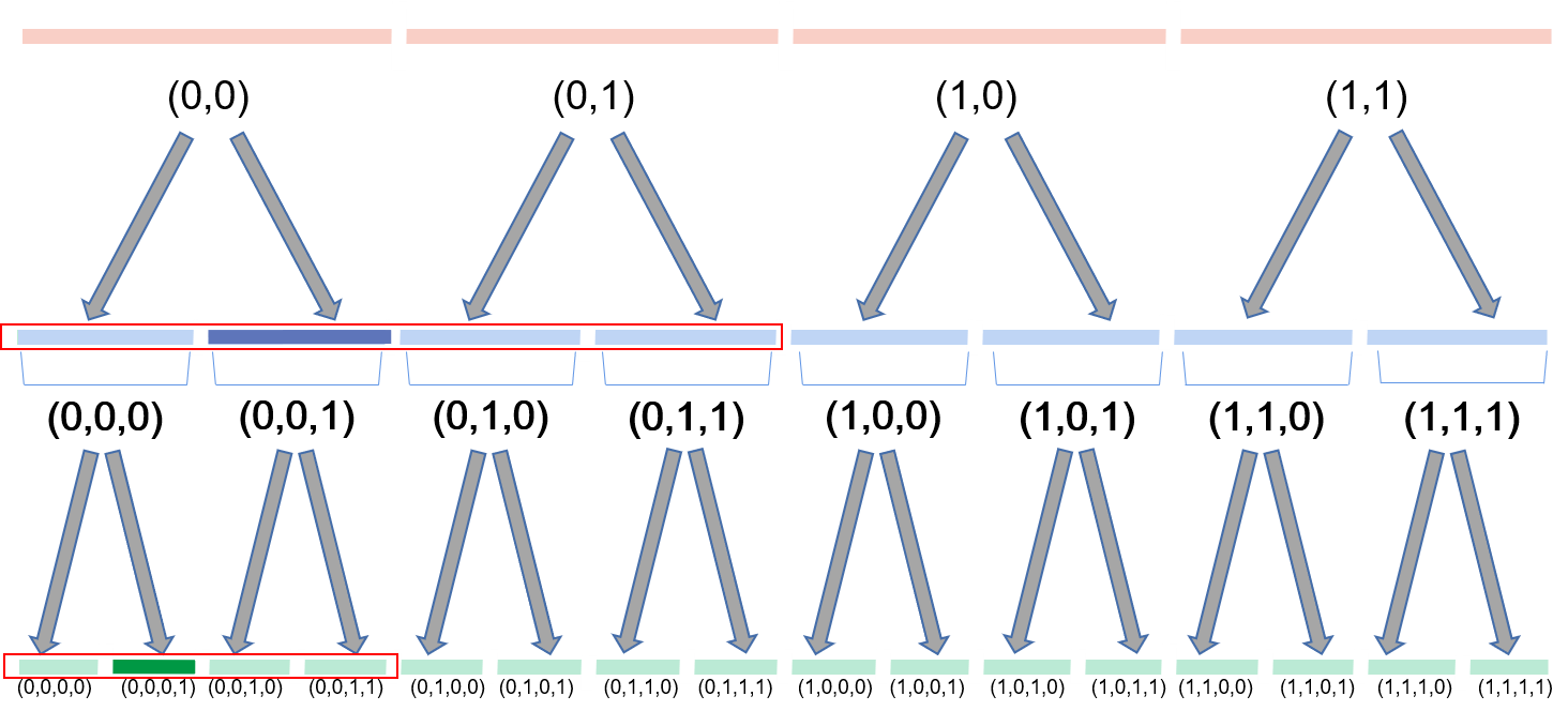
The hierarchically nested attention in Algorithm 1 resembles the celebrated hierarchical matrix method (Hackbusch, 2015), in particular, the $\mathscr{H}^{2}$ matrix from the perspective of matrix operations. In the following, we take the one dimensinoal binary tree-like hierarchical discretization shown in Figure6 as an example to illustrate the reduce operation, decompose operation, and multilevel token aggregation in Algorithm 1 using matrix representations.

Figure 6: Hierarchical discretization of 1D domain. The coarsest level partition is plotted as the top four segments in pink. The segment $(0,0)$ is further partitioned into two child segments $(0,0,0)$ and $(0,0,1)$. During the reducing process, the computation proceeds from bottom to top to obtain coarser level representations. For example, the $(0,0)$ representations are obtained by applying learnable reduce operations $\mathcal{R}^{(2)}$ and $\mathcal{R}^{(1)}$ on $(0,0,0)$ and $(0,0,1)$ respectively. When generating the high-resolution representations, the computation proceeds from top to bottom by applying learnable decomposition operations $\mathcal{D}^{(1)}$ and $\mathcal{D}^{(2)}.$ The red frames show examples of attention windows at each level.

STEP 0: Given features ${\bm{f}}^{(r)}$, compute the queries $\bm{q}_{i}^{(r)}$, keys $\bm{k}_{j}^{(r)}$, and values $\bm{v}_{i}^{(r)}$ for $j\in\mathcal{I}^{(r)}$.

Starting from the finest level features ${\bm{f}}_{i}^{(r)},i\in\mathcal{I}^{(r)}$, the queries $\bm{q}^{(r)}$ can be obtained by

$$\left[\begin{array}[]{c}\vdots\\ \bm{q}_{i}^{(r)}\\ \vdots\end{array}\right]=\underbrace{\left[\begin{array}[]{llll}{\bm{W}}^{Q,(r)}&&\\ &{\bm{W}}^{Q,(r)}&&\\ &&\ddots&\\ &&&{\bm{W}}^{Q,(r)}\end{array}\right]}_{|\mathcal{I}^{(r)}|}\left.\left[\begin{array}[]{c}\vdots\\ {\bm{f}}_{i}^{(r)}\\ \vdots\end{array}\right]\right\}|\mathcal{I}^{(r)}|,$$

the keys $\bm{k}^{(r)}$ and values $\bm{v}^{(r)}$ can follow the similar procedure.

STEP 1: For $m=r-1:1$, Do the reduce operations $\bm{q}_{i}^{(m)}=\mathcal{R}^{(m)}(\{\bm{q}_{j}^{(m+1)}\}_{j\in i^{(m,m+1)}})$ and also for $\bm{k}_{i}^{(m)}$ and $\bm{v}_{i}^{(m)}$, for any $i\in\mathcal{I}^{(m)}$.
If $\mathcal{R}^{(m)}$ is linear, the reduce operations correspond to $\left[\begin{array}[]{c}\vdots\\ \bm{q}_{i}^{(m)}\\ \vdots\end{array}\right]={{\bm{\mathsfit{R}}}^{(m)}}\left[\begin{array}[]{c}\vdots\\ \bm{q}_{i}^{(m+1)}\\ \vdots\end{array}\right]$.The reduce matrix is given by

$${{\bm{\mathsfit{R}}}^{(m)}}:=\underbrace{\left[\begin{array}[]{llllllll }{\bm{R}}_{0}^{(m)}&{\bm{R}}_{1}^{(m)}&&&&&&\\ &&{\bm{R}}_{0}^{(m)}&{\bm{R}}_{1}^{(m)}\\ &&&&\ddots&\ddots&\\ &&&&&&{\bm{R}}_{0}^{(m)}&{\bm{R}}_{1}^{(m)}\end{array}\right]}_{|\mathcal{I}^{(m+1)}|}\left.\begin{array}[]{c}\cr\\ \cr\\ \cr\\ \end{array}\right\}|\mathcal{I}^{(m)}|,$$

and ${\bm{R}}_{0}^{(m)},{\bm{R}}_{1}^{(m)}\in\mathbb{R}^{\mathcal{C}{(m-1)}\times\mathcal{C}{(m)}}$ are matrices parametrized by linear layers in our paper (in practice, queries, keys, and values use different ${\bm{R}}_{0}^{(m)},{\bm{R}}_{1}^{(m)}$ to enhance the expressivity). In general, these operators $\mathcal{R}^{(m)}$ are not limited to linear operators. The composition of nonlinear activation functions would help increase the expressivity. The nested learnable operators $\mathcal{R}^{(m)}$ also induce the channel mixing and is equivalent to a structured parameterization of ${\bm{W}}^{Q},{\bm{W}}^{V},{\bm{W}}^{K}$ matrices for the coarse level tokens, in the sense that, inductively, $\left[\begin{array}[]{c}\vdots\\ \bm{q}_{i}^{(m)}\\ \vdots\end{array}\right]={{\bm{\mathsfit{R}}}^{(m)}}\cdots{{\bm{\mathsfit{R}}}^{(r-1)}}\left[\begin{array}[]{c}\vdots\\ \bm{q}_{i}^{(r)}\\ \vdots\end{array}\right]={{\bm{\mathsfit{R}}}^{(m)}}\cdots{{\bm{\mathsfit{R}}}^{(r-1)}}\left[\begin{array}[]{llll}{\bm{W}}^{Q,(r)}&&\\ &{\bm{W}}^{Q,(r)}&&\\ &&\ddots&\\ &&&{\bm{W}}^{Q,(r)}\end{array}\right]\left[\begin{array}[]{c}\vdots\\ \bm{f}_{i}^{(r)}\\ \vdots\end{array}\right].$

STEP 2: With the $m$-th level queries and keys, we can calculate the local attention matrix ${\bm{G}}_{\rm loc}^{(m)}$ at $m$-th level with $G^{(m)}_{\rm{loc},i,j}:=\exp(\bm{q}_{i}^{(m)}\cdot\bm{k}_{j}^{(m)})$ for $i\in\mathcal{N}^{(m)}(j)$, or $i\sim j$.

STEP 3: The decompose operations, opposite to the reduce operations, correspond to the transpose of the following matrix in the linear case,

$${{\bm{\mathsfit{D}}}^{(m)}}:=\underbrace{\left[\begin{array}[]{llllllll }{\bm{D}}_{0}^{(m)}&{\bm{D}}_{1}^{(m)}&&&&&&\\ &&{\bm{D}}_{0}^{(m)}&{\bm{D}}_{1}^{(m)}\\ &&&&\ddots&\ddots&\\ &&&&&&{\bm{D}}_{0}^{(m)}&{\bm{D}}_{1}^{(m)}\end{array}\right]}_{|\mathcal{I}^{(m+1)}|}\left.\begin{array}[]{c}\cr\\ \cr\\ \cr\\ \end{array}\right\}|\mathcal{I}^{(m)}|,$$

The $m$-th level aggregation in Figure 3 contributes to the final output ${{\bm{f}}}^{(r)}$ in the form ${\bm{\mathsfit{D}}}^{(r-1),{\bm{\mathsfit{T}}}}\cdots{\bm{\mathsfit{D}}}^{(m),{\bm{\mathsfit{T}}}}{\bm{G}}_{\rm loc}^{(m)}{\bm{\mathsfit{R}}}^{(m)}\cdots{\bm{\mathsfit{R}}}^{(r-1)}\left[\begin{array}[]{c}\vdots\\ \bm{v}_{i}^{(r)}\\ \vdots\end{array}\right]$. Eventually, aggregations at all $r$ levels in one V cycle can be summed up as

$$\left[\begin{array}[]{c}\vdots\\ {\bm{h}}_{i}^{(r)}\\ \vdots\end{array}\right]=\left(\sum_{m=1}^{r-1}({\bm{\mathsfit{D}}}^{(r-1),{\bm{\mathsfit{T}}}}\cdots{\bm{\mathsfit{D}}}^{(m),{\bm{\mathsfit{T}}}}{\bm{G}}_{loc}^{(m)}{\bm{\mathsfit{R}}}^{(m)}\cdots{\bm{\mathsfit{R}}}^{(r-1)})+{\bm{G}}_{\rm loc}^{(r)}\right)\left[\begin{array}[]{c}\vdots\\ \bm{v}_{i}^{(r)}\\ \vdots\end{array}\right].$$ (4)

The hierarchical attention matrix ${\bm{G}}_{h}:=\sum_{m=1}^{r-1}({\bm{\mathsfit{D}}}^{(r-1),{\bm{\mathsfit{T}}}}\cdots{\bm{\mathsfit{D}}}^{(m),{\bm{\mathsfit{T}}}}{\bm{G}}_{loc}^{(m)}{\bm{\mathsfit{R}}}^{(m)}\cdots{\bm{\mathsfit{R}}}^{(r-1)})+{\bm{G}}_{\rm loc}^{(r)}$ in equation 4 resembles the three-level $\mathscr{H}^{2}$ matrix decomposition illustrated in Figure 7. We refer to Hackbusch (2015) for a detailed description. The sparsity of ${\bm{G}}_{h}$ lies in the fact that the attention matrix is only computed for pairs of tokens within the neighbor set. The $\mathscr{H}^{2}$ matrix-vector multiplication in equation 4 implies the $\mathcal{O}(N)$ complexity of Algorithm 1.

Figure 7: A demonstration of the decomposition of attention matrix into three levels of local attention matrix.

Note that, the local attention matrix at level $\mathcal{I}^{(1)}$ (pink), level $\mathcal{I}^{(2)}$ (blue) and level $\mathcal{I}^{(3)}$ (green ) are ${\bm{G}}_{loc}^{(1)}$, ${\bm{G}}_{loc}^{(2)}$ and ${\bm{G}}_{loc}^{(3)}$, respectively. However, when considering their contributions to the finest level, they are equivalent to the attention matrix ${\bm{\mathsfit{D}}}^{(2),{\bm{\mathsfit{T}}}}{\bm{\mathsfit{D}}}^{(1),{\bm{\mathsfit{T}}}}{\bm{G}}_{loc}^{(1)}{\bm{\mathsfit{R}}}^{(1)}{\bm{\mathsfit{R}}}^{(2)}\in\mathbb{R}^{\mathcal{I}^{(3)}}\times\mathbb{R}^{\mathcal{I}^{(3)}}$ (pink), ${\bm{\mathsfit{D}}}^{(2),{\bm{\mathsfit{T}}}}{\bm{G}}_{loc}^{(2)}{\bm{\mathsfit{R}}}^{(2)}\in\mathbb{R}^{\mathcal{I}^{(3)}}\times\mathbb{R}^{\mathcal{I}^{(3)}}$ (blue) and ${\bm{G}}_{loc}^{(3)}$ (green), as demonstrated in Figure 7. Each pink block and blue block are actually low-rank sub-matrices with rank $\mathcal{C}^{(1)}$ and rank $\mathcal{C}^{(2)}$, respectively, by definition.

Appendix C Proof of Proposition 3.3

Proof.

For each level $m$, the cost to compute equation 2 is $c(|\mathcal{I}^{(m)}|\mathcal{C}^{(m)})$ since for each $i\in\mathcal{I}^{(m)}$ the cardinality of the neighbour set $\mathcal{N}^{(m)}(i)$ is bounded by a constant $c$. The reduce operation ${\bm{f}}_{i}^{(k-1)}=\mathcal{R}^{(k-1)}(\{{\bm{f}}_{j}^{(m)}\}_{j\in i^{(k-1,k)}})$ costs at most $|\mathcal{I}^{(m)}|\mathcal{C}^{(m)}\mathcal{C}^{(k-1)}$ flops and so does the decompose operation at the same level. Therefore, for each level, the operation cost is $c(|\mathcal{I}^{(m)}|\mathcal{C}^{(m)})+2|\mathcal{I}^{(m)}|\mathcal{C}^{(m)}\mathcal{C}^{(m-1)}$. When $\mathcal{I}$ is a quadtree, $\mathcal{I}^{(r)}=N,\,\mathcal{I}^{(r-1)}=N/4,\cdots,\mathcal{I}^{(1)}=4$, therefore the total computational cost $\sim\mathcal{O}(N)$. ∎

Appendix D More Examples for Spectral Bias in Multiscale Operator Learning

In Figure 1, we demonstrate the spectral bias of Fourier Neural Operators and show the superiority of HANO through the multiscale trigonometric benchmark. We provide more details in this section due to limited space in the main text.

D.1 Comparison of Solutions/Derivatives for More Neural Operators

We show the coefficient, reference solution from Multiscale trigonometric dataset, and the comparison with other operator learning models such as Galerkin Transformer (GT), SWIN, and multiwavelet neural operator (MWT) in Figure 8. HANO not only predicts the function values more accurately than the other models, but more importantly, it captures the fine scale oscillations more accurately, as reflected by the predicted derivatives in (d) of Figure 8.

(a) coefficient in $\log_{10}$ scale

(b) reference solution in 2D

(c) 1D slices of the predicted solutions

(d) 1D slices of the predicted solution derivatives

Figure 8: (a) multiscale trigonometric coefficient, (b) reference solution, (c) comparison of predicted solutions on the slice $x=0$, (d) comparison of predicted derivative $\frac{\partial u}{\partial y}$ on the slice $x=0$.

D.2 Comparison of Error Spectrum for More Neural Operators

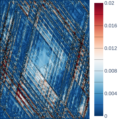
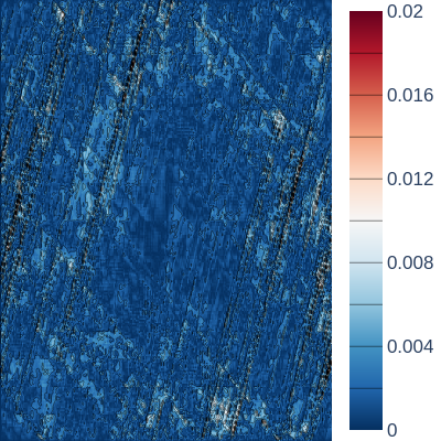
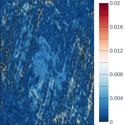
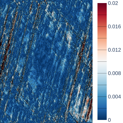
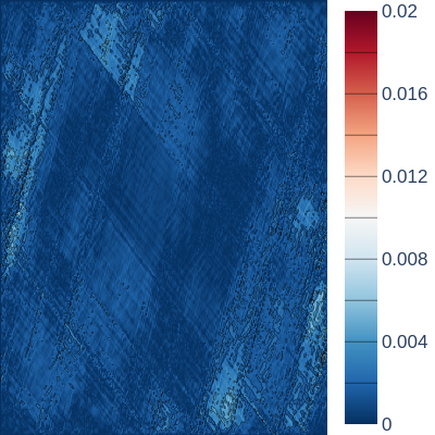
In Figs. 1 (c) and (d), we decompose the error into the frequency domain $[-256\pi,256\pi]^{2}$ and plot the absolute error spectrum for HANO and FNO. Here, in 9, we also include the absolute error and absolute error spectrum for more state-of-the-art models, such as multiwavelet neural operator (MWT), Galerkin Transformer (GT), and SWIN. The comprehensive comparison also demonstrates that existing methods exhibit spectral bias to some degree. This analysis also explains, from another perspective, why HANO achieves the best performance.

(a) FNO

(b) MWT

(c) GT

(d) SWIN

(e) HANO

(f) FNO

(g) MWT

(h) GT

(i) SWIN

(j) HANO

Figure 9: Top: (a)-(e) absolute error of different operator learning methods; Bottom: (f)-(j) absolute error spectrum in $\log_{10}$ scale of different opeator learning methods.

D.3 Training Dynamics in the Frequency Domain

To better illustrate the spectral bias of multiscale operator learning, we show the training dynamics in the frequency domain. Recall that, we discretize the spatial domain $D=[0,1]^{2}$ uniformly with $h=1/n$ and use the grid $\mathsf{G}^{2}:=\{(x_{i},x_{j})=(ih,jh)\mid i,j=0,\dots,n_{f}-1\}$ in our experiments. For any $\xi\in\mathbb{Z}_{n}^{2}:=\left\{\xi\in\mathbb{Z}^{2}\mid-n/2+1\leqslant\xi_{j}\leqslant n/2,j=1,2\right\},$ the normalized discrete Fourier transform (DFT) coefficients of $f$ writes $\mathcal{F}(f)(\xi):=\frac{1}{\sqrt{n}}\sum_{x\in\mathsf{G}^{2}}f(x)e^{-2i\pi x\cdot\xi}$. Then the prediction error in terms of frequency $\xi\in\mathbb{Z}_{n}^{2}$ is measured by

$$\mathcal{E}^{\mathrm{train}}(\mathcal{N};\xi):={\frac{1}{N}}\sum_{i=1}^{N_{train}}|\mathcal{F}(\bm{u}_{i}^{\mathrm{train}}-\mathcal{N}(\bm{a}_{i}^{\mathrm{train}}))(\xi)|,$$

$$\mathcal{E}^{\mathrm{test}}(\mathcal{N};\xi):={\frac{1}{N}}\sum_{i=1}^{N_{\mathrm{test}}}|\mathcal{F}(\bm{u}_{i}^{\mathrm{test}}-\mathcal{N}(\bm{a}_{i}^{test}))(\xi)|.$$

where $\{\bm{a}_{i}^{\mathrm{train}},\bm{u}_{i}^{\mathrm{train}}\}_{i=1}^{N_{\mathrm{train}}}$ and $\{\bm{a}_{i}^{\mathrm{test}},\bm{u}_{i}^{\mathrm{test}}\}_{i=1}^{N_{\mathrm{test}}}$ are the training and testing datasets of Darcy rough task. For low frequencies $\xi$, $\mathcal{E}(\mathcal{N};\xi)$ represents the capability of the neural network for predicting the global trend. Conversely, for high frequencies $\xi$, $\mathcal{E}(\mathcal{N};\xi)$ represents the capability for predicting variations on small scales. During training, we record $\mathcal{E}^{\mathrm{train}}(\mathcal{N};\xi)$ and $\mathcal{E}^{\mathrm{test}}(\mathcal{N};\xi)$ for each $\xi$ at each epoch.

From Figure 10, we conclude that existing methods struggle with learning high frequencies. UNet and UNO mitigate this to some extent, likely due to their UNet-like multi-level structure. HANO’s error decays faster for higher frequencies and more uniformly overall. It also achieves lower testing errors. The mathematical foundations of MWT, UNet, and UNO can be attributed to multigrid methods (Xu & Zikatanov, 2017) and wavelet-based multiresolution methods (Brewster & Beylkin, 1995; Beylkin & Coult, 1998). However, these methods may have limitations for multiscale PDEs (Branets et al., 2009) because they apply uniform operations regardless of the input data structure. In contrast, self-attention and data-driven reduce/decompose operations in the HANO architecture may address this limitation by adapting to the input data.

(a) FNO

(b) MWT

(c) UNet

(d) UNO

(e) HANO

(f) FNO

(g) MWT

(h) UNet

(i) UNO

(j) HANO

Figure 10: Top: (a)-(e) show the training error dynamics in the frequency domain. The x-axis shows the first 12 dominating frequencies, from low frequency (left) to high frequency (right). The y-axis shows the number of training epochs. The colorbar shows the normalized $L^{2}$ error (with respect to the error at epoch 0) in $\log_{10}$ scale. We compare five different methods; Bottom: (f)-(j) Corresponding testing error dynamics in the frequency domain for different methods.

Appendix E Implementation Details

We provide implementation details in this section.

E.1 Architecture

In the HANO implementation, we follow the window attention scheme in Liu et al. (2021b) for the definition of the neighborhood $\mathcal{N}^{(\cdot)}(\cdot)$ in equation 2. In this paper, we choose $r=3$ as the depth of the HANO, GeLU as the activation function, and a CNN-based patch embedding module to transfer the input data into features/tokens.

For a dataset with resolution $n_{f}\times n_{f}$, such as in the multiscale elliptic equation benchmark 4.2, the input feature ${\bm{f}}^{(3)}$ is represented as a tensor of size $n\times n\times C$ via patch embedding. The self-attention is first computed within a local window on level 3. Then the reduce layer concatenates the features of each group of $2\times 2$ neighboring tokens and applies a linear transformation on the $4C$-dimensional concatenated features on $\frac{n}{2}\times\frac{n}{2}$ level 2 tokens, to obtain level 2 features ${\bm{f}}^{(2)}$ as a tensor of the size $\frac{n}{2}\times\frac{n}{2}\times 2C$. The procedure is repeated from level 2 to level 1 with ${\bm{f}}^{(1)}$ of size $\frac{n}{4}\times\frac{n}{4}\times 4C$.

For the decompose operations, starting at level 1, a linear layer is applied to transform the $4C$-dimensional features ${\bm{f}}^{(1)}$ into $8C$-dimensional features. Each level 1 token with $8C$-dimensional features is decomposed into four level 2 tokens with $2C$-dimensional features. These four level 2 tokens are added to the existing level 2 feature ${\bm{f}}^{(2)}$ with output size of $\frac{n}{2}\times\frac{n}{2}\times 2C$. The decomposition procedure is repeated from level 2 to level 3. The output of level 3 is ${\bm{f}}^{(3)}$, which has a size of $n\times n\times C$. We call the above procedures a cycle and we repeat $k$ cycles by the same set up with layer normalizations between cycles.

We summarize the detailed configuration for HANO-l in Table 1. The variants of HANO mainly differ by the channel dimension. For example, HANO-l has 64, 128, 256 channels per level, while HANO-s has 24, 48, 96 channels per level.

Module	Hyperparameters
Patch embedding	patch size: 4, padding: 0
Hierarchical Attention	$\begin{array}[]{c}\textsc{number of levels: }3\\ \textsc{down sampling ratio}\frac{|\mathcal{I}^{m+1}|}{|\mathcal{I}^{m}|}:4\\ \textsc{feature dimension at each level: }\{64,128,256\}\\ \textsc{window size at each level: }\{4,4,4\}\\ \textsc{LayerNorm position: after attention}\\ \textsc{number of cycles: 2}\end{array}$

Table 4: Hyperparameter Configuration

E.2 Training Setup

We apply the Adam optimizer with learning rate $1\mathrm{e}{-3}$, weight decay $1\mathrm{e}{-4}$ and the 1-cycle schedule as in Cao (2021). We choose batch size 8 for experiments in Sections 4.2 and 4.3, and batch size 4 for experiments in Appendices A.1.1 and F.2.

For the Darcy rough case, we use a split of 1280, 112, and 112, respectively, with a max of 500 epochs. For Darcy smooth and multiscale trigonometric cases, we use a split of 1000, 100, and 100, respectively, with a max of 500 epochs for the Darcy smooth case and 300 for the multiscale trigonometric case.

All experiments are run on a NVIDIA A100 GPU.

E.3 Hyperparameter Study

Model	$H^{1}$ $(\times 10^{-2})$	$L^{2}$ $(\times 10^{-2})$
HANO [3, 8, 80]	1.843	0.648
HANO [3, 8, 128]	1.761	0.688
HANO [3, 4, 80]	1.898	0.710
HANO [3, 4, 64]	1.909	0.695
HANO [3, 2, 80]	2.030	0.707

Table 5: Hyperparameter study.

We conduct studies for hyperparameters such as number of hierarchical levels (depth), window size, and feature dimension. We list the results for the Darcy rough benchmark in Table 5, where the notation HANO [3, 8, 80] represents HANO with depth of 3, window size of 8, and feature dimension at the finest level of 80. The experiments are run for 100 epochs.

The results show that larger values of hierarchical level, window size, and feature dimension could help to improve performance, though at a higher computational cost. To balance model size, computational cost, and performance, we choose the hyperparameters as [3, 4, 64] for our final model.

E.4 Memory Usage

We report the memory usage of different models for the Darcy smooth (with resolution 211$\times$211) and Darcy rough (with resolution 256$\times$256) benchmarks in Table 6. The table shows that the memory usage of HANO remains stable across resolutions. For the higher resolution of 256$\times$256, both MWT and GT consume more CUDA memory than HANO, even though HANO achieves much higher accuracy.

Model	Darcy smooth	Darcy rough
FNO	$0.72$	$1.04$
GT	$1.40$	$4.53$
MWT	—	$1.27$
HANO-s	$1.23$	$1.85$
HANO-l	$3.31$	$4.96$

Table 6: The memory usage(GB) of different models by using torchinfo.

Appendix F Additional Experiments

We provide additional experiments in this section.

F.1 Training Dynamics

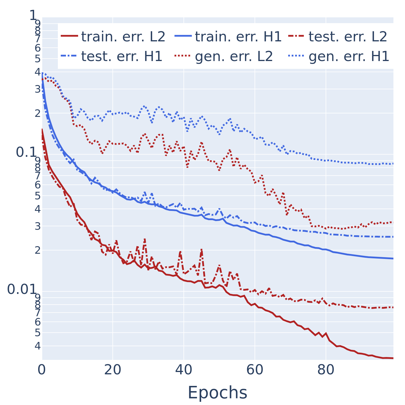
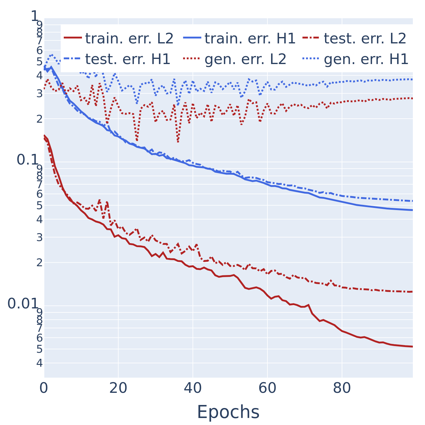
We present the dynamics of training and testing error over 100 epochs of training in Figure 11. We compare HANO trained with $H^{1}$ and $L^{2}$ loss functions, and show the evolution of errors as well as the loss curves during the training process. The comparison shows that HANO with $H^{1}$ loss achieves lower training and testing errors. It also suggests that the $H^{1}$ loss function reduces the generalization gap (measured by the difference between training error and testing error), while $L^{2}$ loss function fails to do so.

(a) Training curve by using $H^{1}$ loss

(b) Training curve by using $L^{2}$ loss

Figure 11: Comparison of training dynamics between HANO trained with $H^{1}$ loss and $L^{2}$ loss

F.2 Helmholtz equation

We test the performance of HANO for the acoustic Helmholtz equation in highly heterogeneous media as an example of multiscale wave phenomena, whose solution is considerably expensive for complicated and large geological models. We adopt the setup from De Hoop et al. (2022), for the Helmholtz equation on the domain $D=[0,1]^{2}$. Given frequency $\omega=10^{3}$ and wavespeed field $c:\Omega\rightarrow\mathbb{R}$, the excitation field $u:\Omega\rightarrow\mathbb{R}$ solves the equation

$$\left\{\begin{aligned} \left(-\Delta-\frac{\omega^{2}}{c^{2}(x)}\right)u&=0&&\text{ in }\Omega,\\ \frac{\partial u}{\partial n}&=0&&\text{ on }\partial\Omega_{1},\partial\Omega_{2},\partial\Omega_{4},\\ \frac{\partial u}{\partial n}&=1&&\text{ on }\partial\Omega_{3},\end{aligned}\right.$$

where $\partial\Omega_{3}$ is the top side of the boundary, and $\partial\Omega_{1,2,4}$ are other sides. The wave speed field is $c(x)=20+\tanh(\tilde{c}(x))$, where $\tilde{c}$ is sampled from the Gaussian field $\tilde{c}\sim\mathcal{N}(0,\left(-\Delta+\tau^{2}\right)^{-d})$, where $\tau=3$ and $d=2$ are chosen to control the roughness. The Helmholtz equation is solved on a $100\times 100$ grid by finite element methods. We aim to learn the mapping from ${\bm{c}}\in\mathbb{R}^{100\times 100}$ to ${\bm{u}}\in\mathbb{R}^{100\times 100}$ as shown in Figure 12.

(a) wavespeed field ${\bm{c}}$

(b) excitation field ${\bm{u}}$

(c) HANO prediction $\hat{{\bm{u}}}$

Figure 12: The mapping ${\bm{c}}\mapsto{\bm{u}}$

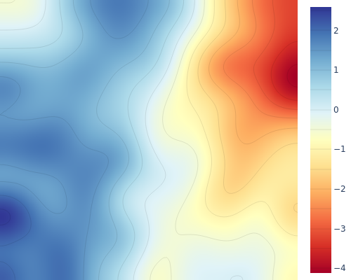
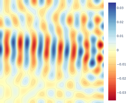
The Helmholtz equation is notoriously difficult to solve numerically. One reason is the so-called resonance phenomenon when the frequency $\omega$ is close to an eigenfrequency of the Helmholtz operator for some particular wave speed $c$. We found that it was necessary to use a large training dataset of size $8000$ examples. The test dataset contained $800$ examples. All models were trained for 500 epochs.

Model	#Parameters	Evaluation time (ms)	$L^{2}$ relative error $(\times 10^{-2})$
FNO	3,282,068	5.8	2.301
UNet	17,261,825	0.1	42.90
HANO	47,632,003	3.0	0.687

Table 7: HANO outperforms the other models by a wide margin. The error of FNO is comparable with the reported results in De Hoop et al. (2022). We note that the four models benchmarked for the Helmholtz equation in De Hoop et al. (2022), including FNO and DeepONet, failed to reach an error less than $1\times 10^{-2}$.

We also compare the evaluation time of the trained models in Table 7. Compared to HANO, FNO has both a larger error and takes longer to evaluate. UNet, as a CNN based method, can evaluate much faster (30 times faster than HANO) but has the worst error (60 times higher than HANO).

F.3 Comparison with classical methods (FDM) and multiscale methods (GRPS)

We compare the accuracy and efficiency of HANO with two conventional solvers: finite difference method (FDM) as a typical classical method, and generalized rough polyharmonic splines (GRPS) (Liu et al., 2021a) as a typical multiscale method. We implement FDM and GRPS in MATLAB and measure the solution time on a CPU (Intel(R) Core(TM) i7-10510U CPU @ 2.30 GHz). We measure the evaluation time of HANO on the CPU and NVIDIA A100 GPU, seperately. The reference solution is defined on a $512\times 512$ grid, sampled from the test dataset. FDM solves the problem on a $256\times 256$ grid. GRPS uses coarse bases of dimension $256^{2}$ to solve the same problem. HANO learns the solution operator on the same resolution as FDM and GRPS. The results are listed in Table 8. Compared with classical methods, HANO has comparable accuracy but significantly less evaluation time.

Model	Evaluation time (s)	Relative $L^{2}$ error ($\times 10^{-2}$)
FDM	0.34	0.84
GRPS	18.9	0.02
HANO(GPU)	0.003	0.58
HANO(CPU)	0.22	0.58

Table 8: Relative $L^{2}$ error and evaluation time on the Darcy rough benchmark.

F.4 Discretization invariance

FNO achieves discretization invariance through Fourier interpolation, enabling models trained on low-resolution data to handle high-resolution input. By incorporating suitable interpolation operators, HANO can achieve a comparable capability. Specifically, it can be trained on lower resolution data but evaluated at higher resolution, without requiring any higher resolution data during training (achieving zero-shot super-resolution).

We conducted the experiments following the same setup as in Li et al. (2021) for the multiscale trigonometric coefficient benchmark. The models were trained on $64\times 64$, $128\times 128$, and $256\times 256$ resolutions, and tested on $128\times 128$, $256\times 256$, and $512\times 512$ resolutions, respectively. Results in Table 9 show that HANO incorporating linear interpolation is more stable than FNO.

	FNO			HANO
	$128$	$256$	$512$	$128$	$256$	$512$
$64$	$5.2808$	$7.9260$	$9.1054$	$1.3457$	$1.3557$	$1.3624$
$128$		$3.9753$	$6.0156$		$0.6715$	$0.6835$
$256$			$3.1871$			$0.5941$

Table 9: Comparison of discretization invariance property for HANO and FNO for the multiscale trigonometric coefficient benchmark. The relative $L^{2}$ error ($\times 10^{-2}$) with respect to the reference solution on the testing resolution is measured.

References

- Bebendorf (2005) M. Bebendorf. Efficient inversion of the galerkin matrix of general second-order elliptic operators with nonsmooth coefficients. Math. Comp., 74(251):1179–1199, 2005.
- Berlyand & Owhadi (2010) L. Berlyand and H. Owhadi. Flux norm approach to finite dimensional homogenization approximations with non-separated scales and high contrast. Arch. Ration. Mech. Anal., 198(2):677–721, 2010.
- Beylkin & Coult (1998) G. Beylkin and N. Coult. A multiresolution strategy for reduction of elliptic PDEs and eigenvalue problems. Appl. Comput. Harmon. Anal., 5(2):129–155, 1998. ISSN 1063-5203.
- Bhattacharya et al. (2021) Kaushik Bhattacharya, Bamdad Hosseini, Nikola B Kovachki, and Andrew M Stuart. Model reduction and neural networks for parametric pdes. The SMAI journal of computational mathematics, 7:121–157, 2021.
- Branets et al. (2009) L. V. Branets, S. S. Ghai, L. L., and X.-H. Wu. Challenges and technologies in reservoir modeling. Commun. Comput. Phys., 6(1):1–23, 2009.
- Brewster & Beylkin (1995) M. E. Brewster and G. Beylkin. A multiresolution strategy for numerical homogenization. Appl. Comput. Harmon. Anal., 2(4):327–349, 1995. ISSN 1063-5203.
- Budninskiy et al. (2019) Max Budninskiy, Houman Owhadi, and Mathieu Desbrun. Operator-adapted wavelets for finite-element differential forms. Journal of Computational Physics, 388:144–177, 2019.
- Cao (2021) Shuhao Cao. Choose a transformer: Fourier or galerkin. Advances in Neural Information Processing Systems, 34, 2021.
- Choromanski et al. (2020) Krzysztof Choromanski, Valerii Likhosherstov, David Dohan, Xingyou Song, Andreea Gane, Tamas Sarlos, Peter Hawkins, Jared Davis, Afroz Mohiuddin, Lukasz Kaiser, et al. Rethinking attention with performers. arXiv preprint arXiv:2009.14794, 2020.
- De Hoop et al. (2022) Maarten De Hoop, Daniel Zhengyu Huang, Elizabeth Qian, and Andrew M Stuart. The cost-accuracy trade-off in operator learning with neural networks. arXiv preprint arXiv:2203.13181, 2022.
- Dosovitskiy et al. (2020) Alexey Dosovitskiy, Lucas Beyer, Alexander Kolesnikov, Dirk Weissenborn, Xiaohua Zhai, Thomas Unterthiner, Mostafa Dehghani, Matthias Minderer, Georg Heigold, Sylvain Gelly, et al. An image is worth 16x16 words: Transformers for image recognition at scale. arXiv preprint arXiv:2010.11929, 2020.
- E & Engquist (2003) Weinan E and B. Engquist. Multiscale modeling and computation. Notices Amer. Math. Soc., 50(9):1062–1070, 2003.
- Engquist & Souganidis (2008) B. Engquist and P. E. Souganidis. Asymptotic and numerical homogenization. Acta Numerica, 17:147–190, 2008.
- Fan et al. (2019a) Yuwei Fan, Jordi Feliu-Fabá, Lin Lin, Lexing Ying, and Leonardo Zepeda-Nunez. A multiscale neural network based on hierarchical nested bases. Res. Math. Sci., 6(21), 2019a.
- Fan et al. (2019b) Yuwei Fan, Lin Lin, Lexing Ying, and Leonardo Zepeda-Núnez. A multiscale neural network based on hierarchical matrices. Multiscale Modeling & Simulation, 17(4):1189–1213, 2019b.
- Greengard & Rokhlin (1987) L. Greengard and V. Rokhlin. A fast algorithm for particle simulations. J. Comput. Phys., 73(2):325–348, 1987.
- Gupta et al. (2021) Gaurav Gupta, Xiongye Xiao, and Paul Bogdan. Multiwavelet-based operator learning for differential equations. Advances in Neural Information Processing Systems, 34:24048–24062, 2021.
- Hackbusch (1985) W. Hackbusch. Multigrid Methods and Applications, volume 4 of Springer Series in Computational Mathematics. Springer-Verlag, Berlin, 1985.
- Hackbusch (2015) Wolfgang Hackbusch. Hierarchical matrices: algorithms and analysis. Springer, Berlin, 2015.
- Hackbusch et al. (2002) Wolfgang Hackbusch, Lars Grasedyck, and Steffen Börm. An introduction to hierarchical matrices. In Proceedings of Equadiff 10, pp. 101–111. Masaryk University, 2002.
- Hauck & Peterseim (2022) Moritz Hauck and Daniel Peterseim. Multi-resolution localized orthogonal decomposition for helmholtz problems. Multiscale Model. Simul., 20(2):657–684, 2022.
- He et al. (2016) Kaiming He, Xiangyu Zhang, Shaoqing Ren, and Jian Sun. Deep residual learning for image recognition. In Proceedings of the IEEE Conference on Computer Vision and Pattern Recognition, pp. 770–778, 2016.
- Ho & Ying (2016) K. Ho and L. Ying. Hierarchical interpolative factorization for elliptic operators: Differential equations. Communiations on Pure and Applied Mathematics, 69(8):1415–1451, 2016.
- Hou et al. (1999) T. Y. Hou, X.-H. Wu, and Z. Cai. Convergence of a multiscale finite element method for elliptic problems with rapidly oscillating coefficients. Math. Comp., 68(227):913–943, 1999.
- Khoo et al. (2020) Yuehaw Khoo, Jianfeng Lu, and Lexing Ying. Solving parametric pde problems with artificial neural networks. European Journal of Applied Mathematics, 32(3):421–435, 2020.
- Kovachki et al. (2021) Nikola Kovachki, Samuel Lanthaler, and Siddhartha Mishra. On universal approximation and error bounds for fourier neural operators. Journal of Machine Learning Research, 22:Art–No, 2021.
- Kovachki et al. (2023) Nikola Kovachki, Zongyi Li, Burigede Liu, Kamyar Azizzadenesheli, Kaushik Bhattacharya, Andrew Stuart, and Anima Anandkumar. Neural operator: Learning maps between function spaces with applications to pdes. Journal of Machine Learning Research, 24(89):1–97, 2023. URL http://jmlr.org/papers/v24/21-1524.html.
- Lanthaler et al. (2022) Samuel Lanthaler, Siddhartha Mishra, and George E Karniadakis. Error estimates for deeponets: A deep learning framework in infinite dimensions. Transactions of Mathematics and Its Applications, 6(1):tnac001, 2022.
- Li et al. (2021) Zongyi Li, Nikola Kovachki, Kamyar Azizzadenesheli, Burigede Liu, Kaushik Bhattacharya, Andrew Stuart, and Anima Anandkumar. Fourier neural operator for parametric partial differential equations. The International Conference on Learning Representations, 2021.
- Liu et al. (2021a) Xinliang Liu, Lei Zhang, and Shengxin Zhu. Generalized rough polyharmonic splines for multiscale pdes with rough coefficients. arXiv preprint arXiv:2103.01788, 2021a.
- Liu et al. (2021b) Ze Liu, Yutong Lin, Yue Cao, Han Hu, Yixuan Wei, Zheng Zhang, Stephen Lin, and Baining Guo. Swin transformer: Hierarchical vision transformer using shifted windows. In Proceedings of the IEEE/CVF International Conference on Computer Vision, pp. 10012–10022, 2021b.
- Lu et al. (2021) Lu Lu, Pengzhan Jin, Guofei Pang, Zhongqiang Zhang, and George Em Karniadakis. Learning nonlinear operators via deeponet based on the universal approximation theorem of operators. Nature Machine Intelligence, 3(3):218–229, 2021.
- Målqvist & Peterseim (2014) A. Målqvist and D. Peterseim. Localization of elliptic multiscale problems. Math. Comp., 83(290):2583–2603, 2014.
- Nguyen et al. (2021) Tan Nguyen, Vai Suliafu, Stanley Osher, Long Chen, and Bao Wang. Fmmformer: Efficient and flexible transformer via decomposed near-field and far-field attention. Advances in neural information processing systems, 34:29449–29463, 2021.
- Owhadi (2017) H. Owhadi. Multigrid with Rough Coefficients and Multiresolution Operator Decomposition from Hierarchical Information Games. SIAM Rev., 59(1):99–149, 2017.
- Owhadi & Zhang (2007) H. Owhadi and L. Zhang. Metric-based upscaling. Comm. Pure Appl. Math., 60(5):675–723, 2007.
- Peng et al. (2021) Hao Peng, Nikolaos Pappas, Dani Yogatama, Roy Schwartz, Noah A Smith, and Lingpeng Kong. Random feature attention. arXiv preprint arXiv:2103.02143, 2021.
- Rahaman et al. (2019) Nasim Rahaman, Devansh Arpit, Aristide Baratin, Felix Draxler, Min Lin, Fred A Hamprecht, Yoshua Bengio, and Aaron Courville. On the spectral bias of deep neural networks. International Conference on Machine Learning, 2019.
- Rahman et al. (2022) Md Ashiqur Rahman, Zachary E Ross, and Kamyar Azizzadenesheli. U-no: U-shaped neural operators. arXiv e-prints, pp. arXiv–2204, 2022.
- Ronen et al. (2019) Basri Ronen, David Jacobs, Yoni Kasten, and Shira Kritchman. The convergence rate of neural networks for learned functions of different frequencies. In Advances in Neural Information Processing Systems, volume 32, pp. 4761–4771, 2019.
- Ronneberger et al. (2015) Olaf Ronneberger, Philipp Fischer, and Thomas Brox. U-net: Convolutional networks for biomedical image segmentation. In International Conference on Medical image computing and computer-assisted intervention, pp. 234–241. Springer, 2015.
- Stachenfeld et al. (2022) Kim Stachenfeld, Drummond Buschman Fielding, Dmitrii Kochkov, Miles Cranmer, Tobias Pfaff, Jonathan Godwin, Can Cui, Shirley Ho, Peter Battaglia, and Alvaro Sanchez-Gonzalez. Learned simulators for turbulence. In International Conference on Learning Representations, 2022.
- Vaswani et al. (2017) Ashish Vaswani, Noam Shazeer, Niki Parmar, Jakob Uszkoreit, Llion Jones, Aidan N Gomez, Lukasz Kaiser, and Illia Polosukhin. Attention is all you need. Advances in neural information processing systems, 30, 2017.
- Wang et al. (2020a) Rui Wang, Karthik Kashinath, Mustafa Mustafa, Adrian Albert, and Rose Yu. Towards physics-informed deep learning for turbulent flow prediction. In Proceedings of the 26th ACM SIGKDD International Conference on Knowledge Discovery & Data Mining, pp. 1457–1466, 2020a.
- Wang et al. (2020b) S. Wang, B.Z. Li, M. Khabsa, H. Fang, and H. Ma. Linformer: Self-attention with linear complexity. arXiv:2006.04768, 2020b.
- Xie et al. (2019) H. Xie, L. Zhang, and H. Owhadi. Fast eigenpairs computation with operator adapted wavelets and hierarchical subspace corrections. SIAM Journal on Numerical Analysis, 57(6):2519–2550, 2019. preprint.
- Xiong et al. (2021) Yunyang Xiong, Zhanpeng Zeng, Rudrasis Chakraborty, Mingxing Tan, Glenn Fung, Yin Li, and Vikas Singh. Nyströmformer: A nyström-based algorithm for approximating self-attention. In Proceedings of the AAAI Conference on Artificial Intelligence, volume 35, pp. 14138–14148, 2021.
- Xu & Zikatanov (2017) Jinchao Xu and Ludmil Zikatanov. Algebraic multigrid methods. Acta Numerica, 26:591–721, 2017.
- Xu et al. (2020) Zhi-Qin John Xu, Yaoyu Zhang, Tao Luo, Yanyang Xiao, and Zheng Ma. Frequency Principle: Fourier Analysis Sheds Light on Deep Neural Networks. Communications in Computational Physics, 28(5):1746–1767, 2020.
- Yu et al. (2022) Annan Yu, Yunan Yang, and Alex Townsend. A quadrature perspective on frequency bias in neural network training with nonuniform data. arXiv preprint arXiv:2205.14300, 2022.
- Zhang et al. (2022) Zizhao Zhang, Han Zhang, Long Zhao, Ting Chen, , Sercan Ö. Arık, and Tomas Pfister. Nested hierarchical transformer: Towards accurate, data-efficient and interpretable visual understanding. In AAAI Conference on Artificial Intelligence (AAAI), 2022.
- Zhao et al. (2022) Jiawei Zhao, Robert Joseph George, Yifei Zhang, Zongyi Li, and Anima Anandkumar. Incremental fourier neural operator. arXiv preprint arXiv:2211.15188, 2022.
- Zhu & Zabaras (2018) Yinhao Zhu and Nicholas Zabaras. Bayesian deep convolutional encoder–decoder networks for surrogate modeling and uncertainty quantification. J. Comput. Phys., 366:415–447, 2018.