Vacuum-dual static perfect fluid obeying $p=-(n-3)\rho/(n+1)$ in $n(\geq 4)$ dimensions

Hideki Maeda

Department of Electronics and Information Engineering, Hokkai-Gakuen University, Sapporo 062-8605, Japan.

h-maeda@hgu.jp

Abstract

We obtain the general $n(\geq 4)$-dimensional static solution with an $(n-2)$-dimensional Einstein base manifold for a perfect fluid obeying a linear equation of state $p=-(n-3)\rho/(n+1)$. It is a generalization of Semiz’s four-dimensional general solution with spherical symmetry and consists of two different classes. Through the Buchdahl transformation, the class-I and class-II solutions are dual to the topological Schwarzschild-Tangherlini-(A)dS solution and one of the $\Lambda$-vacuum direct-product solutions, respectively. While the metric of the spherically symmetric class-I solution is $C^{\infty}$ at the Killing horizon for $n=4$ and $5$, it is $C^{1}$ for $n\geq 6$ and then the Killing horizon turns to be a parallelly propagated curvature singularity. For $n=4$ and $5$, the spherically symmetric class-I solution can be attached to the Schwarzschild-Tangherlini vacuum black hole with the same value of the mass parameter at the Killing horizon in a regular manner, namely without a lightlike massive thin-shell. This construction allows new configurations of an asymptotically (locally) flat black hole to emerge. If a static perfect fluid hovers outside a vacuum black hole, its energy density is negative. In contrast, if the dynamical region inside the event horizon of a vacuum black hole is replaced by the class-I solution, the corresponding matter field is an anisotropic fluid and may satisfy the null and strong energy conditions. While the latter configuration always involves a spacelike singularity inside the horizon for $n=4$, it becomes a non-singular black hole of the big-bounce type for $n=5$ if the ADM mass is larger than a critical value.

1 Introduction

The study of static and spherically symmetric solutions with a perfect fluid in general relativity aims to find nice models representing compact objects in gravitational equilibrium such as white dwarfs or neutron stars. Based on the Tolman-Oppenheimer-Volkoff (TOV) equation [1, 2], a huge effort has been made in the history of general relativity to obtain physically reasonable solutions with a regular center that are asymptotically flat or can be attached in a regular manner at some radius to an exterior Schwarzschild vacuum region.

In the last century, exact solutions had been obtained mainly in a heuristic way by introducing nice coordinate systems or variables. (See [3] for the results until 1998 and also Sec. 16.1 in the textbook [4].) In the 21st century, based on the earlier observations [5, 6, 7], an algorithm to construct all regular static spherically symmetric perfect-fluid solutions based on the generating function has been developed without specifying an equation of state [8, 9, 10]. This development lead to derive an infinite number of previously unknown physically interesting exact solutions as well as to establish solution-generating methods [10, 11, 12, 13]. The solution space has also been studied in the dynamical systems approach with linear and polytropic equations of state [14, 15].

Nevertheless, a complete classification of static spherically symmetric solutions obeying a physically important linear equation of state $p=\chi\rho$ has not been achieved yet except for several particular values of $\chi$. (The dominant energy condition is equivalent to $\rho\geq 0$ with $-1\leq\chi\leq 1$ in arbitrary dimensions [16].) For example, such a static solution is absent for $\chi=0$ and the general solution consists of the Schwarzschild-(A)dS and Nariai solutions for $\chi=-1$ by Birkhoff’s theorem. Ivanov studied the integrability of the field equations in detail for general $\chi$ in four dimensions and obtained a particular solution for $\chi=-1/5$ by the Buchdahl transformation from the (anti-)de Sitter solution as a seed solution [17]. In this situation, Semiz classified solutions with a mass function given as a polynomial of the areal radius [18]. Based on this result, he has recently derived the general static and spherically symmetric perfect-fluid solution for $\chi=-1/5$ [19]. Semiz’s general solution consists of two different classes and they are related to the Schwarzschild-(A)dS and Nariai $\Lambda$-vacuum solutions through the Buchdahl transformation [19]. Some properties of this general solution have been studied in [20]. However, there still remains room for investigation to understand these solutions and provide their physical interpretations.

In this paper, we will therefore fully investigate Semiz’s general solution in a broader framework. To be more precise, we will derive and study the general $n(\geq 4)$-dimensional static solution with an $(n-2)$-dimensional Einstein base manifold for $\chi=-(n-3)/(n+1)$. The motivation for studying the case with negative pressure in arbitrary dimensions is not to find a model of a star-like static equilibrium configuration, but to gain insight into the nature of gravity through the analysis of exact solutions. In fact, since a static equilibrium is realized by balancing the pressure with self-gravity, a static solution with negative $\chi$ should have a negative energy density violating the weak energy condition and/or admit a (naked) singularity. Furthermore, a perfect fluid with negative pressure generally suffers from the hydrodynamical instability in the flat spacetime because the speed of sound $c_{\rm s}:=\sqrt{{\rm d}p/{\rm d}\rho}$ becomes pure imaginary. Note, however, that $\chi=-1$ is an exception because such a perfect fluid is equivalent to a cosmological constant and its energy density and pressure are constant.

The present paper is organized as follows. First, in Sec. 2, we will generalize Semiz’s four-dimensional spherically symmetric perfect-fluid solutions to $n(\geq 4)$ dimensions with a more general base manifold of the Einstein space characterized by a curvature scalar $k(=1,0,-1)$. Furthermore, we will show that the generalized Semiz solutions are dual to the topological Schwarzschild-Tangherlini-(A)dS solution or one of the $\Lambda$-vacuum direct-product solutions through the $n$-dimensional Buchdahl transformation. In Sec. 3, we will fully investigate physical and geometric properties of the $n$-dimensional Semiz class-I solution with spherical symmetry. We will summarize our results and present concluding remarks in the final section. Our conventions for curvature tensors are $[\nabla_{\rho},\nabla_{\sigma}]V^{\mu}={{R}^{\mu}}_{\nu\rho\sigma}V^{\nu}$ and ${R}_{\mu\nu}={{R}^{\rho}}_{\mu\rho\nu}$, where Greek indices run over all spacetime indices. The signature of the Minkowski spacetime is $(-,+,+,\cdots,+)$ and other types of indices will be specified in the main text. We adopt the units such that $c=1$ and $\kappa_{n}:=8\pi G_{n}$, where $G_{n}$ is the $n$-dimensional gravitational constant. Throughout the paper, a prime over a function denotes differentiation with respect to its argument.

2 Semiz-class perfect-fluid solutions in $n(\geq 4)$ dimensions

In this section, we drive exact solutions to the following Einstein equations with a perfect fluid in $n(\geq 4)$ dimensions:

$${\cal E}_{\mu\nu}:=G_{\mu\nu}-\kappa_{n}T_{\mu\nu}=0,$$ (2.1)

$${T}_{\mu\nu}=(\rho+p)u_{\mu}u_{\nu}+pg_{\mu\nu}.$$ (2.2)

Here $\rho$ and $p$ are the energy density and pressure of a perfect fluid, respectively, and $u^{\mu}$ is the normalized $n$-velocity of the fluid element satisfying $u_{\mu}u^{\mu}=-1$.

To write down the Einstein equations (2.1), consider an $n(\geq 4)$-dimensional spacetime $({\cal M}^{n},g_{\mu\nu})$ as a warped product of a two-dimensional Lorentzian spacetime $(M^{2},g_{AB})$ and an $(n-2)$-dimensional Einstein space $(K_{(k)}^{n-2},\gamma_{ij})$ with the following metric:

$$\begin{aligned} {\rm d}s^{2}=&g_{\mu\nu}{\rm d}x^{\mu}{\rm d}x^{\nu}\\ =&g_{AB}(y){\rm d}y^{A}{\rm d}y^{B}+\sigma(y)^{2}\gamma_{ij}(z){\rm d}z^{i}{\rm d}z^{j},\end{aligned}$$ (2.3)

where $A,B=0,1$ and $i,j=2,3,\cdots,n-1$. The Ricci tensor on $K_{(k)}^{n-2}$ is given by ${}^{(n-2)}{R}_{ij}=k(n-3)\gamma_{ij}$ with $k=1,0,-1$. For the spacetime (2.3), the Riemann tensor is decomposed as

$${R}_{ABCD} ={}^{(2)}{R}_{ABCD},$$ (2.4)

$${R}_{AiBj} =-\sigma(D_{A}D_{B}\sigma)\gamma_{ij},$$ (2.5)

$${R}_{ijkl} =\sigma^{2}[k-(D\sigma)^{2}](\gamma_{ik}\gamma_{jl}-\gamma_{il}\gamma_{jk}),$$ (2.6)

where ${}^{(2)}{R}_{ABCD}$ and $D_{A}$ are the Riemann tensor and the covariant derivative on $M^{2}$, respectively, and $(D\sigma)^{2}:=g^{AB}(D_{A}\sigma)(D_{B}\sigma)$. Also, the Einstein tensor is decomposed as

$$G_{AB}= -(n-2)\sigma^{-1}D_{A}D_{B}\sigma$$

$$+\frac{1}{2}g_{AB}\biggl{\{}2(n-2)\sigma^{-1}D^{2}\sigma-(n-2)(n-3)\sigma^{-2}[k-(D\sigma)^{2}]\biggl{\}},$$ (2.7)

$$G_{ij}= \gamma_{ij}\biggl{\{}-\frac{1}{2}\sigma^{2}({}^{(2)}{R})+(n-3)\sigma D^{2}\sigma-\frac{1}{2}(n-3)(n-4)[k-(D\sigma)^{2}]\biggl{\}},$$ (2.8)

where ${}^{(2)}{R}$ is the Ricci scalar on $M^{2}$ and $D^{2}\sigma:=g^{AB}D_{A}D_{B}\sigma$. (See Appendix A in [21] for derivation.)

In general relativity, the generalized Misner-Sharp quasi-local mass [22, 23] is defined for the spacetime (2.3) as

$$m_{\rm MS}:=\frac{(n-2)V_{n-2}^{(k)}}{2\kappa_{n}}\sigma^{n-3}[k-(D\sigma)^{2}],$$ (2.9)

where a constant $V_{n-2}^{(k)}$ denotes the volume of $K_{(k)}^{n-2}$ if it is compact. Among the basic properties of $m_{\rm MS}$ studied in [24, 21], we will use the fact that $m_{\rm MS}$ converges to the ADM mass at spacelike infinity in an asymptotically flat spacetime.

2.1 Exact solutions for $p=-(n-3)\rho/(n+1)$

Now we derive the general solution for an equation of state $p=-(n-3)\rho/(n+1)$ by adopting the following comoving coordinates:

$$\begin{aligned} &{\rm d}s^{2}=-\frac{\alpha(x)}{\beta(x)}{\rm d}t^{2}+\beta(x)^{-2(n-4)/(n-3)}\biggl{(}\frac{\beta(x)}{\alpha(x)}{\rm d}x^{2}+x^{2}\beta(x)^{2}\gamma_{ij}{\rm d}z^{i}{\rm d}z^{j}\biggl{)},\\ &u^{\mu}\frac{\partial}{\partial x^{\mu}}=\sqrt{\frac{\beta}{\alpha}}\frac{\partial}{\partial t}.\end{aligned}$$ (2.10)

This is a static spacetime in the domain with $\alpha>0$ and $\beta>0$ or $\alpha<0$ and $\beta<0$. However, since the powers of $\beta$ in the metric are integers for $n=4$ and $5$ and rational numbers for $n\geq 6$, the domain with $\alpha<0$ and $\beta<0$ are allowed only for $n=4$ and $5$. The author has discovered the metric ansatz (2.10) by trial and error based on the experience of performing a complete classification of solutions in the Einstein-Maxwell system in [25].

With the metric (2.10), a combination $-(n-3){{\cal E}^{t}}_{t}-(n-5){{\cal E}^{x}}_{x}+2(n-2){{\cal E}^{2}}_{2}=0$ of the Einstein equations (2.1) gives

$$\kappa_{n}\{(n-3)\rho+(n+1)p\}=(n-2)x^{-1}\beta^{(n-5)/(n-3)}\left\{x\alpha^{\prime\prime}+(n-2)\alpha^{\prime}\right\}.$$ (2.11)

With an equation of state $(n-3)\rho+(n+1)p=0$, the above equation is integrated to give

$$\alpha(x)=\alpha_{0}+\frac{\alpha_{1}}{x^{n-3}},$$ (2.12)

where $\alpha_{0}$ and $\alpha_{1}$ are integration constants. Substituting Eq. (2.12) into a combination ${{\cal E}^{x}}_{x}-{{\cal E}^{2}}_{2}=0$, we obtain the following master equation for $\beta(x)$:

$$0= \biggl{\{}(n-4)\alpha_{0}+\frac{(n-2)\alpha_{1}}{x^{n-3}}\biggl{\}}x\beta^{\prime}+\biggl{(}\alpha_{0}+\frac{\alpha_{1}}{x^{n-3}}\biggl{)}x^{2}\beta^{\prime\prime}+2(n-3)(k-\alpha_{0}\beta).$$ (2.13)

The general solution to Eq. (2.13) for $\alpha_{0}\neq 0$ is

$$\beta(x)=\frac{k}{\alpha_{0}}+\frac{\eta}{x^{n-3}}-\zeta x^{2}\biggl{(}\alpha_{0}+\frac{\alpha_{1}}{x^{n-3}}\biggl{)}^{(n-1)/(n-3)},$$ (2.14)

where $\eta$ and $\zeta$ are integration constants. The general solution to Eq. (2.13) for $\alpha_{0}=0$ (and then $\alpha_{1}\neq 0$ is required) is

$$\beta(x)=\beta_{0}+\frac{\beta_{1}}{x^{n-3}}-\frac{k}{(n-3)\alpha_{1}}x^{n-3},$$ (2.15)

where $\beta_{0}$ and $\beta_{1}$ are integration constants. The signs of the functions $\alpha(x)$ and $\beta(x)$ are determined by the values of the parameters $\alpha_{0}$, $\alpha_{1}$, $\eta$, $\zeta$, $\beta_{0}$, and $\beta_{1}$, and we focus on spacetimes with a Lorentzian metric.

2.1.1 Semiz class-I solution

The metric functions in Eq. (2.10) and the corresponding energy density $\rho$ of the general solution for $\alpha_{0}\neq 0$ are given by

$$\begin{aligned} &\alpha(x)=\alpha_{0}+\frac{\alpha_{1}}{x^{n-3}},\qquad\beta(x)=\frac{k}{\alpha_{0}}+\frac{\eta}{x^{n-3}}-\zeta x^{2}\biggl{(}\alpha_{0}+\frac{\alpha_{1}}{x^{n-3}}\biggl{)}^{(n-1)/(n-3)},\\ &\rho=-\frac{n+1}{n-3}p=\frac{(n^{2}-1)(n-2)\alpha_{0}^{2}\zeta}{2(n-3)\kappa_{n}}\frac{\alpha(x)^{2/(n-3)}}{\beta(x)^{2/(n-3)}}.\end{aligned}$$ (2.16)

We refer to this solution as the Semiz class-I solution. This solution for $n=4$ and $k=1$ corresponds to Semiz’s solution for $C_{1}\neq 0$ [19] and its particular case with $\alpha_{1}=\alpha_{0}^{2}\eta$ was obtained by Ivanov by the Buchdahl transformation from the (anti-)de Sitter solution [17]. (See the vacuum dual (2.41) to the Semiz class-I solution below.)

To see that Eq. (2.16) is actually a two-parameter family of solutions, we perform coordinate transformations $(t,x)\to({\bar{t}},{\bar{x}})$ such that ${\bar{t}}=(n-3)|\alpha_{0}|t$ and ${\bar{x}}=(\alpha_{0}x^{n-3}+\alpha_{1})/[(n-3)^{2}|\alpha_{0}|^{2}]$ together with redefinitions of the parameters ${\bar{\eta}}:=\eta-k\alpha_{1}/\alpha_{0}^{2}$ and ${\bar{\zeta}}:=\zeta(n-3)^{2(n-1)/(n-3)}|\alpha_{0}|^{2(n-1)/(n-3)}$. Then the Semiz class-I solution is written as

$$\begin{aligned} &{\rm d}s^{2}=-\frac{{\bar{x}}}{{\bar{\beta}}({\bar{x}})}{\rm d}{\bar{t}}^{2}+{\bar{\beta}}({\bar{x}})^{-2(n-4)/(n-3)}\biggl{(}\frac{{\bar{\beta}}({\bar{x}})}{{\bar{x}}}{\rm d}{\bar{x}}^{2}+{\bar{\beta}}({\bar{x}})^{2}\gamma_{ij}{\rm d}z^{i}{\rm d}z^{j}\biggl{)},\\ &\rho=-\frac{n+1}{n-3}p=\frac{(n^{2}-1)(n-2){\bar{\zeta}}}{2(n-3)^{3}\kappa_{n}}\frac{{\bar{x}}^{2/(n-3)}}{{\bar{\beta}}({\bar{x}})^{2/(n-3)}},\\ &{\bar{\beta}}({\bar{x}}):=x({\bar{x}})^{n-3}\beta(x({\bar{x}}))={\bar{\eta}}+k(n-3)^{2}{\bar{x}}-{\bar{\zeta}}{\bar{x}}^{(n-1)/(n-3)},\end{aligned}$$ (2.17)

which is characterized by two parameters ${\bar{\eta}}$ and ${\bar{\zeta}}$. The expression (2.17) shows that $\rho$ blows when ${\bar{\beta}}({\bar{x}})=0$ holds for ${\bar{\zeta}}\neq 0$.

For $k=\pm 1$, the solution (2.17) in the vacuum limit ${\bar{\zeta}}\to 0$ is expressed by coordinate transformations ${\bar{t}}=k\tau/(n-3)$ and $r=[{\bar{\eta}}+k(n-3)^{2}{\bar{x}}]^{1/(n-3)}$ and a redefinition of the parameter $2M:=k{\bar{\eta}}$ as

$$\begin{aligned} &{\rm d}s^{2}=-\biggl{(}k-\frac{2M}{r^{n-3}}\biggl{)}{\rm d}\tau^{2}+\biggl{(}k-\frac{2M}{r^{n-3}}\biggl{)}^{-1}{\rm d}r^{2}+r^{2}\gamma_{ij}{\rm d}z^{i}{\rm d}z^{j}.\end{aligned}$$ (2.18)

This is the topological Schwarzschild-Tangherlini solution. We note that ${\tilde{M}}:=(n-2)V_{n-2}^{(k)}M/\kappa_{n}$ coincides with the generalized Misner-Sharp mass (2.9). For $k=0$, the form (2.17) admits the following vacuum limit ${\bar{\zeta}}\to 0$:

$${\rm d}s^{2}=-\frac{{\bar{x}}}{{\bar{\eta}}}{\rm d}{\bar{t}}^{2}+\frac{{\bar{\eta}}^{-(n-5)/(n-3)}}{{\bar{x}}}{\rm d}{\bar{x}}^{2}+{\bar{\eta}}^{2/(n-3)}\gamma_{ij}{\rm d}z^{i}{\rm d}z^{j}.$$ (2.19)

This is the Ricci-flat direct-product solution, which is a direct product spacetime ${\rm M}_{2}\times K_{(0)}^{n-2}$ of a two-dimensional Minkowski spacetime ${\rm M}_{2}$ and an $(n-2)$-dimensional Ricci-flat space $K_{(0)}^{n-2}$.

Probably, the best expression of the Semiz class-I solution for $k=\pm 1$ is obtained from the metric (2.10) with Eq. (2.16) by coordinate transformations $(t,x)\to({\tilde{t}},r)$ such that $t=(k/\alpha_{0}){\tilde{t}}$ and $x^{n-3}=(r^{n-3}-\eta)\alpha_{0}/k$ together with redefinitions of the parameters $2M:=k(\eta-k\alpha_{1}/\alpha_{0}^{2})$ and ${\tilde{\zeta}}:=\zeta(\alpha_{0}^{2}/k^{2})^{(n-1)/(n-3)}$. Then the solution becomes

$$\begin{aligned} &{\rm d}s^{2}=-f(r){\rm d}{\tilde{t}}^{2}+h(r)^{-2(n-4)/(n-3)}\biggl{(}f(r)^{-1}{\rm d}r^{2}+r^{2}h(r)^{2}\gamma_{ij}{\rm d}z^{i}{\rm d}z^{j}\biggl{)},\\ &\rho=-\frac{n+1}{n-3}p=\frac{(n^{2}-1)(n-2)k^{2}{\tilde{\zeta}}}{2(n-3)\kappa_{n}}f(r)^{2/(n-3)}\end{aligned}$$ (2.20)

with

$$f(r)=\frac{kr^{n-3}-2M}{r^{n-3}-{\tilde{\zeta}}\left(kr^{n-3}-2M\right)^{(n-1)/(n-3)}},$$ (2.21)

$$h(r)=1-\frac{{\tilde{\zeta}}}{r^{n-3}}\left(kr^{n-3}-2M\right)^{(n-1)/(n-3)}.$$ (2.22)

Although the coordinate transformations are singular, this form of the solution is valid also for $k=0$. The form (2.20) clearly shows that the vacuum limit ${\tilde{\zeta}}\to 0$ is the topological Schwarzschild-Tangherlini solution (2.18) for any $k$. The solution (2.20) with $k=0$ is also given by Eq. (2.18) with $k=0$, which is shown by further coordinate transformations.

2.1.2 Semiz class-II solution

The metric functions in Eq. (2.10) and the corresponding energy density $\rho$ of the general solution for $\alpha_{0}=0$ (and then $\alpha_{1}\neq 0$) are given by

$$\begin{aligned} &\alpha(x)=\frac{\alpha_{1}}{x^{n-3}},\qquad\beta(x)=\beta_{0}+\frac{\beta_{1}}{x^{n-3}}-\frac{k}{(n-3)\alpha_{1}}x^{n-3},\\ &\rho=-\frac{n+1}{n-3}p=\frac{(n+1)(n-2)k}{2\kappa_{n}x^{2}\beta(x)^{2/(n-3)}}.\end{aligned}$$ (2.23)

We refer to this solution as the Semiz class-II solution. This solution for $n=4$ and $k=1$ corresponds to Semiz’s solution for $C_{1}=0$ [19].

For $\beta_{0}\neq 0$, by coordinate transformations $(t,x)\to({\bar{t}},r)$ such that ${\bar{t}}=\beta_{0}^{-1}t$ and $r^{n-3}=\beta_{0}x^{n-3}+\beta_{1}$ together with a redefinition of the parameter $2M=-\alpha_{1}\beta_{0}^{2}$, the solution is written as

$$\begin{aligned} &{\rm d}s^{2}=\frac{2M}{r^{n-3}h(r)}{\rm d}{\bar{t}}^{2}-h(r)^{-2(n-4)/(n-3)}\biggl{(}\frac{r^{n-3}h(r)}{2M}{\rm d}r^{2}-r^{2}h(r)^{2}\gamma_{ij}{\rm d}z^{i}{\rm d}z^{j}\biggl{)},\\ &\rho=-\frac{n+1}{n-3}p=\frac{(n+1)(n-2)k}{2\kappa_{n}r^{2}h(r)^{2/(n-3)}},\\ &h(r):=x(r)^{n-3}\beta(x(r))/r^{n-3}=1+\frac{k(r^{n-3}-\beta_{1})^{2}}{2(n-3)Mr^{n-3}},\end{aligned}$$ (2.24)

which is characterized by two parameters $\beta_{1}$ and $M$. The form (2.24) shows that the Semiz class-II solution with $\beta_{0}\neq 0$ in the vacuum case ($k=0$) is the topological Schwarzschild-Tangherlini solution (2.18) with $k=0$.

For $\beta_{0}=0$ with $\beta_{1}\neq 0$, by coordinate transformations $(t,x)\to({\bar{t}},r)$ such that

$${\bar{t}}=\sqrt{|\alpha_{1}|}|\beta_{1}|^{-(n-1)/[2(n-3)]}t,\qquad r=\frac{x^{n-3}}{(n-3)\sqrt{|\beta_{1}||\alpha_{1}|}},$$ (2.25)

the Semiz class-II solution becomes

$$\begin{aligned} &{\rm d}s^{2}=|\beta_{1}|^{2/(n-3)}\biggl{[}-\frac{1}{{\bar{\beta}}(r)}\frac{\alpha_{1}}{|\alpha_{1}|}{\rm d}{\bar{t}}^{2}+{\bar{\beta}}(r)^{-(n-5)/(n-3)}\frac{|\alpha_{1}|}{\alpha_{1}}{\rm d}r^{2}+{\bar{\beta}}(r)^{2/(n-3)}\gamma_{ij}{\rm d}z^{i}{\rm d}z^{j}\biggl{]},\\ &{\bar{\beta}}(r):=\frac{x(r)^{n-3}\beta(x(r))}{|\beta_{1}|}=\frac{\beta_{1}}{|\beta_{1}|}-k(n-3)\frac{|\alpha_{1}|}{\alpha_{1}}r^{2},\\ &\rho=-\frac{n+1}{n-3}p=\frac{(n+1)(n-2)k}{2\kappa_{n}|\beta_{1}|^{2/(n-3)}{\bar{\beta}}(r)^{2/(n-3)}}.\end{aligned}$$ (2.26)

The form (2.26) shows that the Semiz class-II solution with $\beta_{0}=0$ in the vacuum case ($k=0$) is the Ricci-flat direct-product solution ${\rm M}_{2}\times K_{(0)}^{n-2}$.

Lastly, for $\beta_{0}=\beta_{1}=0$ (and then $k\neq 0$ is required), by coordinate transformations $(t,x)\to({\bar{t}},r)$ such that

$${\bar{t}}=\sqrt{\alpha_{1}}t,\qquad r=\biggl{(}-\frac{k}{(n-3)\alpha_{1}}\biggl{)}^{1/(n-3)}x^{2},$$ (2.27)

the Semiz class-II solution becomes

$$\begin{aligned} &{\rm d}s^{2}=-\frac{1}{r^{n-3}}{\rm d}{\bar{t}}^{2}-\frac{n-3}{4k}{\rm d}r^{2}+r^{2}\gamma_{ij}{\rm d}z^{i}{\rm d}z^{j},\\ &\rho=-\frac{n+1}{n-3}p=\frac{(n+1)(n-2)k}{2\kappa_{n}r^{2}}.\end{aligned}$$ (2.28)

This solution does not admit a vacuum limit and requires $k=-1$ for the Lorentzian signature. Actually, the solution (2.28) is a special case with $\chi=-(n-3)/(n+1)$ of the generalized Tolman-VI solution for an equation of state $p=\chi\rho$ given in Appendix A.

2.2 Semiz-class solutions as vacuum duals

Here we show that the Semiz class solutions are duals to the $\Lambda$-vacuum solutions through the Buchdahl transformation. In particular, the Semiz class-I solution is dual to the topological Schwarzschild-Tangherlini-(A)dS solution given by

$$\begin{aligned} {\rm d}s^{2}=&-f(r){\rm d}t^{2}+f(r)^{-1}{\rm d}r^{2}+r^{2}\gamma_{ij}{\rm d}z^{i}{\rm d}z^{j},\\ f(r)=&k-\frac{2M}{r^{n-3}}-\frac{2\Lambda}{(n-1)(n-2)}r^{2},\end{aligned}$$ (2.29)

while the Semiz class-II solution is dual to the generalized Nariai solution, generalized anti-Nariai solution, and the Ricci-flat direct product solution for $k=1$, $k=-1$, and $k=0$, respectively. The generalized Nariai (anti-Nariai) solution for $k=1$ with $\Lambda>0$ ($k=-1$ with $\Lambda<0$) is a direct-product solution ${\rm dS}_{2}\times K_{(1)}^{n-2}$ (${\rm AdS}_{2}\times K_{(-1)}^{n-2}$) of a two-dimensional de Sitter (anti-de Sitter) spacetime and an $(n-2)$-dimensional Einstein space with positive (negative) Ricci curvature, of which line-element may be written as

$$\begin{aligned} &{\rm d}s^{2}=-f(r){\rm d}t^{2}+f(r)^{-1}{\rm d}r^{2}+\frac{k(n-2)(n-3)}{2\Lambda}\gamma_{ij}{\rm d}z^{i}{\rm d}z^{j},\\ &f(r)=f_{0}+f_{1}r-\frac{2\Lambda}{n-2}r^{2},\end{aligned}$$ (2.30)

where $f_{0}$ and $f_{1}$ are arbitrary constants.

2.2.1 $n(\geq 4)$-dimensional Buchdahl transformation

Now we present the $n(\geq 4)$-dimensional Buchdahl transformation which map a static solution to another in the system given by Eqs. (2.1) and (2.2) [26]. (See also Sec. 10.11 in the textbook [4] for $n=4$.)

Proposition 1

Suppose that the following set

$$\begin{aligned} &{\rm d}s^{2}=-\Omega(X)^{-2}{\rm d}t^{2}+\Omega(X)^{2/(n-3)}{\bar{g}}_{IJ}(X){\rm d}X^{I}{\rm d}X^{J},\\ &u^{\mu}\frac{\partial}{\partial x^{\mu}}=\Omega\frac{\partial}{\partial t},\qquad\rho=\rho_{0}(X),\qquad p=p_{0}(X)\end{aligned}$$ (2.31)

is a solution to the Einstein equations (2.1) with a perfect fluid (2.2), where the indices $I$ and $J$ run from $1$ to $n-1$. Then, the following set is also a solution:

$$\begin{aligned} &{\rm d}s^{2}=-\Omega(X)^{2}{\rm d}t^{2}+\Omega(X)^{-2/(n-3)}{\bar{g}}_{IJ}(X){\rm d}X^{I}{\rm d}X^{J},\\ &u^{\mu}\frac{\partial}{\partial x^{\mu}}=\Omega^{-1}\frac{\partial}{\partial t},\quad\rho=-\biggl{\{}\rho_{0}+\frac{2(n-1)}{n-3}p_{0}\biggl{\}}{\Omega}^{4/(n-3)},\quad p=p_{0}\Omega^{4/(n-3)}.\end{aligned}$$ (2.32)

Proof. For the metric (2.31), the Einstein tensor $G_{\mu\nu}$ is decomposed as

$${G}{}_{tt}= \frac{1}{2}\Omega^{-2(n-2)/(n-3)}\left\{{\bar{R}}-\frac{2(n-2)}{n-3}{\bar{D}}^{2}\ln\Omega-\frac{n-2}{n-3}({\bar{D}}\ln\Omega)^{2}\right\},$$ (2.33)

$${G}{}_{IJ}= {\bar{G}}_{IJ}-\frac{n-2}{n-3}({\bar{D}}_{I}\ln\Omega)({\bar{D}}_{J}\ln\Omega)+\frac{n-2}{2(n-3)}{\bar{g}}_{IJ}({\bar{D}}\ln\Omega)^{2},$$ (2.34)

where ${\bar{D}}_{I}$ is the covariant derivative with respect to ${\bar{g}}_{IJ}$ and we have defined ${\bar{D}}^{2}:={\bar{g}}^{IJ}{\bar{D}}_{I}{\bar{D}}_{J}$ and $({\bar{D}}\ln\Omega)^{2}:={\bar{g}}^{IJ}({\bar{D}}_{I}\ln\Omega)({\bar{D}}_{J}\ln\Omega)$. Here ${\bar{R}}_{IJ}$, ${\bar{R}}$, and ${\bar{G}}_{IJ}$ are the Ricci tensor, Ricci scalar, and Einstein tensor constructed from ${\bar{g}}_{IJ}$, respectively. (See Appendix A in [27] for derivation.) Then, Eqs. (2.1) and (2.2) for the set (2.31) reduce to the following set of equations:

$$(n-3){\bar{R}}_{IJ}=(n-2)({\bar{D}}_{I}\ln\Omega)({\bar{D}}_{J}\ln\Omega)-2\kappa_{n}p\Omega^{2/(n-3)}{\bar{g}}_{IJ},$$ (2.35)

$$(n-2){\bar{D}}^{2}\ln\Omega=-\kappa_{n}[(n-3)\rho+(n-1)p]\Omega^{2/(n-3)}.$$ (2.36)

The above field equations are invariant under the following transformations:

$$\Omega={\tilde{\Omega}}^{-1},\quad p={\tilde{p}}{\tilde{\Omega}}^{4/(n-3)},\quad\rho=-\biggl{\{}{\tilde{\rho}}+\frac{2(n-1)}{n-3}{\tilde{p}}\biggl{\}}{\tilde{\Omega}}^{4/(n-3)}.$$ (2.37)

 

Proposition 1 is an $n(\geq 4)$-dimensional generalization of the solution-generating transformation presented in [26] for $n=4$. However, since Buchdahl presented the expressions (2.33) and (2.34) for arbitrary $n(\geq 4)$ in a different notation, Proposition 1 should be attributed to him. If a seed solution (2.31) satisfies $p_{0}=\chi\rho_{0}$, the generated solution (2.32) satisfies $p={\tilde{\chi}}\rho$, where

$${\tilde{\chi}}:=-\frac{(n-3)\chi}{(n-3)+2(n-1)\chi}.$$ (2.38)

In particular, $\chi={\tilde{\chi}}$ holds for $\chi(={\tilde{\chi}})=-(n-3)/(n-1)$, for which the strong energy condition is marginally satisfied. (See Eq. (3.44) below with $p_{1}=p_{2}\equiv p$.) It was claimed in [29] that the general spherically symmmetric static solution had been obtained in this case with $n=4$ (hence $\chi=-1/3$). However, a complete proof does not seem to have been given. Another interesting equation of state is $\chi=-(n-3)/[2(n-1)]$, with which the dual solution satisfies $\rho=0$. In this case with $n=4$ (hence $\chi=-1/6$), Semiz constructed a particular static solution with spherical symmetry by the Buchdahl transformation [30].

2.2.2 Vacuum duals to the Semiz-class solutions

Here we adopt the Buchdahl transformation to the Semiz-class solutions. The metric generated by the Buchdahl transformation from the seed metric (2.10) is given by

$${\rm d}s^{2}= -\frac{\beta(x)}{\alpha(x)}{\rm d}t^{2}+\alpha(x)^{2/(n-3)}\biggl{(}\frac{{\rm d}x^{2}}{\alpha(x)\beta(x)}+x^{2}\gamma_{ij}{\rm d}z^{i}{\rm d}z^{j}\biggl{)}.$$ (2.39)

Equation (2.38) shows ${\tilde{\chi}}=-1$ for $\chi=-(n-3)/(n+1)$. Therefore, the Semiz-class solutions are dual to $\Lambda$-vacuum solutions.

Substituting $\alpha(x)$ and $\beta(x)$ of the Semiz-I class solution (2.16) ($\alpha_{0}\neq 0$ is required) to the metric (2.39), the corresponding Einstein tensor is computed to give

$${G^{\mu}}_{\nu}=-\frac{1}{2}(n-1)(n-2)\zeta\alpha_{0}^{2}{\delta^{\mu}}_{\nu},$$ (2.40)

so that its dual is a $\Lambda$-vacuum solution with $\Lambda=(n-1)(n-2)\zeta\alpha_{0}^{2}/2$. By coordinate transformation $t=\alpha_{0}{\bar{t}}$ and $r=(\alpha_{0}x^{n-3}+\alpha_{1})^{1/(n-3)}$, the dual solution is written as

$$\begin{aligned} &{\rm d}s^{2}=-f(r){\rm d}{\bar{t}}^{2}+f(r)^{-1}{\rm d}r^{2}+r^{2}\gamma_{ij}{\rm d}z^{i}{\rm d}z^{j},\\ &f(r)=k-\frac{k\alpha_{1}-\alpha_{0}^{2}\eta}{r^{n-3}}-\alpha_{0}^{2}\zeta r^{2},\end{aligned}$$ (2.41)

which is the topological Schwarzschild-Tangherlini-(A)dS solution (2.29) with $2M=k\alpha_{1}-\alpha_{0}^{2}\eta$ and $\Lambda=(n-1)(n-2)\alpha_{0}^{2}\zeta/2$.

Substituting $\alpha(x)$ and $\beta(x)$ of the Semiz-II class solution (2.23) ($\alpha_{1}\neq 0$ is required) to the metric (2.39), the corresponding Einstein tensor is computed to give

$${G^{\mu}}_{\nu}=-\frac{(n-2)(n-3)k}{2\alpha_{1}^{2/(n-3)}}{\delta^{\mu}}_{\nu},$$ (2.42)

so that its dual is a $\Lambda$-vacuum solution with $\Lambda=(n-2)(n-3)k/(2\alpha_{1}^{2/(n-3)})$. By a coordinate transformation $r=\alpha_{1}^{-(n-4)/(n-3)}x^{n-3}/(n-3)$, the dual solution is written as

$$\begin{aligned} &{\rm d}s^{2}=-h(r){\rm d}t^{2}+h(r)^{-1}{\rm d}r^{2}+\alpha_{1}^{2/(n-3)}\gamma_{ij}{\rm d}z^{i}{\rm d}z^{j},\\ &h(r)=\frac{\beta_{1}}{\alpha_{1}}+\frac{(n-3)\beta_{0}}{\alpha_{1}^{1/(n-3)}}r-\frac{k(n-3)}{\alpha_{1}^{2/(n-3)}}r^{2}\end{aligned}$$ (2.43)

which is the generalized Nariai (anti-Nariai) solution (2.30) for $k=1$ ($k=-1$) with $\Lambda=(n-2)(n-3)k/(2\alpha_{1}^{2/(n-3)})$. For $k=0$, Eq. (2.43) is the Ricci-flat direct-product solution ${\rm M}_{2}\times K_{(0)}^{n-2}$.

3 Properties of the Semiz class-I solution with spherical symmetry

In this section, we study the Semiz class-I solution (2.20) with spherical symmetry, where $K_{(k)}^{n-2}$ is an $(n-2)$-dimensional sphere ${\rm S}^{n-2}$ (and hence $k=1$). Here we present again the solution without tildes for simplicity;

$$\begin{aligned} &{\rm d}s^{2}=-f(r){\rm d}t^{2}+h(r)^{-2(n-4)/(n-3)}f(r)^{-1}{\rm d}r^{2}+r^{2}h(r)^{2/(n-3)}\gamma_{ij}{\rm d}z^{i}{\rm d}z^{j},\\ &\rho=-\frac{n+1}{n-3}p=\frac{(n^{2}-1)(n-2){\zeta}}{2(n-3)\kappa_{n}}f(r)^{2/(n-3)},\end{aligned}$$ (3.1)

where $f$ and $h$ are given by

$$f(r)=\frac{r^{n-3}-2M}{r^{n-3}-{\zeta}\left(r^{n-3}-2M\right)^{(n-1)/(n-3)}},$$ (3.2)

$$h(r)=1-\frac{{\zeta}}{r^{n-3}}\left(r^{n-3}-2M\right)^{(n-1)/(n-3)}.$$ (3.3)

With $\zeta=0$, the solution reduces to the Schwarzschild-Tangherlini vacuum solution and hereafter we assume $\zeta\neq 0$.

For convenience, we introduce a new coordinate $y:=r^{n-3}-2M$, with which the solution (3.1) is written as

$${\rm d}s^{2}=-\frac{y}{\Pi(y)}{\rm d}t^{2}+\frac{\Pi(y)^{-(n-5)/(n-3)}}{(n-3)^{2}y}{\rm d}y^{2}+\Pi(y)^{2/(n-3)}\gamma_{ij}{\rm d}z^{i}{\rm d}z^{j},$$ (3.4)

$$\rho=-\frac{n+1}{n-3}p=\frac{(n^{2}-1)(n-2)\zeta}{2(n-3)\kappa_{n}}\biggl{(}\frac{y}{\Pi(y)}\biggl{)}^{2/(n-3)},$$ (3.5)

$$\Pi(y):=2M+y-\zeta y^{(n-1)/(n-3)}.$$ (3.6)

Hereafter we will study the solution in this coordinate system. First of all, reality of the metric with the Lorentzian signature $(-,+,\cdots,+)$ restricts the domain of $y$. In fact, $\Pi$ must be positive for $n\geq 5$ and, in addition, $y$ must be positive for $n\geq 6$. By these constraints, $y\to\infty$ is allowed for $n=4$ with any $\zeta$ and $n\geq 5$ with $\zeta<0$, while $y\to-\infty$ is allowed for $n=4$ with any $\zeta$ and $n=5$ with $\zeta<0$. Properties of the boundaries $\Pi=0$ and $y=0$ will be studied in the following subsections.

In the spherically symmetric case, we express the volume of ${\rm S}^{n-2}$ as $V_{n-2}^{(1)}={\cal A}_{n-2}$, where ${\cal A}_{n-2}$ is given in terms of the Gamma function $\Gamma(x)$ as

$${\cal A}_{n-2}:=\frac{2\pi^{(n-1)/2}}{\Gamma((n-1)/2)}.$$ (3.7)

Then, with the areal radius $\sigma=\Pi^{1/(n-3)}$, the Misner-Sharp mass (2.9) is computed to give

$$m_{\rm MS}= \frac{(n-2){\cal A}_{n-2}}{2\kappa_{n}}\Pi\left(1-y\Pi^{-1}{\Pi^{\prime}}^{2}\right).$$ (3.8)

In an asymptotically flat spacetime, $m_{\rm MS}$ converges to the ADM mass at spacelike infinity [24, 21]. Although $\lim_{y\to\pm\infty}R^{\mu\nu}_{\phantom{\mu}\phantom{\nu}\rho\sigma}=0$ is satisfied, Eq. (3.8) blows up in the limit of $y\to\pm\infty$ as

$$\lim_{y\to\pm\infty}m_{\rm MS}\simeq -\frac{(n-1)^{2}(n-2){\cal A}_{n-2}\zeta^{2}}{2(n-3)^{2}\kappa_{n}}y^{(n+1)/(n-3)}.$$ (3.9)

Therefore, the spacetime (3.4) with $\zeta\neq 0$ is asymptotically locally flat as $y\to\pm\infty$ if $y$ is a spacelike coordinate in the asymptotic regions.

3.1 Scalar polynomial curvature singularity and metric reality

In the spacetime (3.4) with $M\neq 0$ (and $\zeta\neq 0$), the energy density $\rho$ blows up at $y=y_{\rm s}(\neq 0)$ determined by $\Pi(y_{\rm s})=0$ and therefore it is a scalar polynomial curvature singularity. The relation between $M$ and $y_{\rm s}$ is given by

$$M=\frac{1}{2}\left(-y_{\rm s}+\zeta y_{\rm s}^{(n-1)/(n-3)}\right)=:M_{\rm s}(y_{\rm s}).$$ (3.10)

The constraint $\Pi(y)>0$ for $n\geq 5$ is equivalent to $M>M_{\rm s}(y)$. The forms of $M=M_{\rm s}(y)$ depending on $n$ and the sign of $\zeta$ are drawn in Fig. 1. For $n=4$, there are two extrema at $y=\pm 1/\sqrt{3\zeta}=:y_{{\rm ex}(4\pm)}$ for $\zeta>0$ and we have $M_{\rm s}(y_{4(\pm)})=\mp 1/(3\sqrt{3\zeta})=:M_{\rm ex(4\mp)}$, while $M_{\rm s}(y)$ is monotonically decreasing for $\zeta<0$. For $n=5$, there is a single extremum at $y=1/(2\zeta)=:y_{{\rm ex}(5)}$ and we have $M_{\rm s}(y_{{\rm ex}(5)})=-1/(8\zeta)=:M_{\rm ex(5)}$. For $n\geq 6$, there is a single local minimum at $y=[(n-3)/\{(n-1)\zeta\}]^{(n-3)/2}=:y_{\rm ex}$ for $\zeta>0$ and we have $M_{\rm s}(y_{\rm ex})=-y_{\rm ex}/(n-1)=:M_{\rm ex}$.

In the case of $M=0$, $\Pi(y)=0$ corresponds to $y=0$ or $1-\zeta y^{2/(n-3)}=0$ and the latter is a scalar polynomial curvature singularity. In contrast, the spacetime is analytic at $y=0$ corresponding to the regular center $r=0$ for any $n(\geq 4)$. This fact is obvious in the coordinate system (3.1) with $M=0$:

$${\rm d}s^{2}=-\frac{{\rm d}t^{2}}{1-{\zeta}r^{2}}+(1-{\zeta}r^{2})^{-(n-5)/(n-3)}{\rm d}r^{2}+r^{2}(1-{\zeta}r^{2})^{2/(n-3)}\gamma_{ij}{\rm d}z^{i}{\rm d}z^{j},$$ (3.11)

$$\rho=\frac{(n^{2}-1)(n-2)\zeta}{2(n-3)\kappa_{n}(1-\zeta r^{2})^{2/(n-3)}}.$$ (3.12)

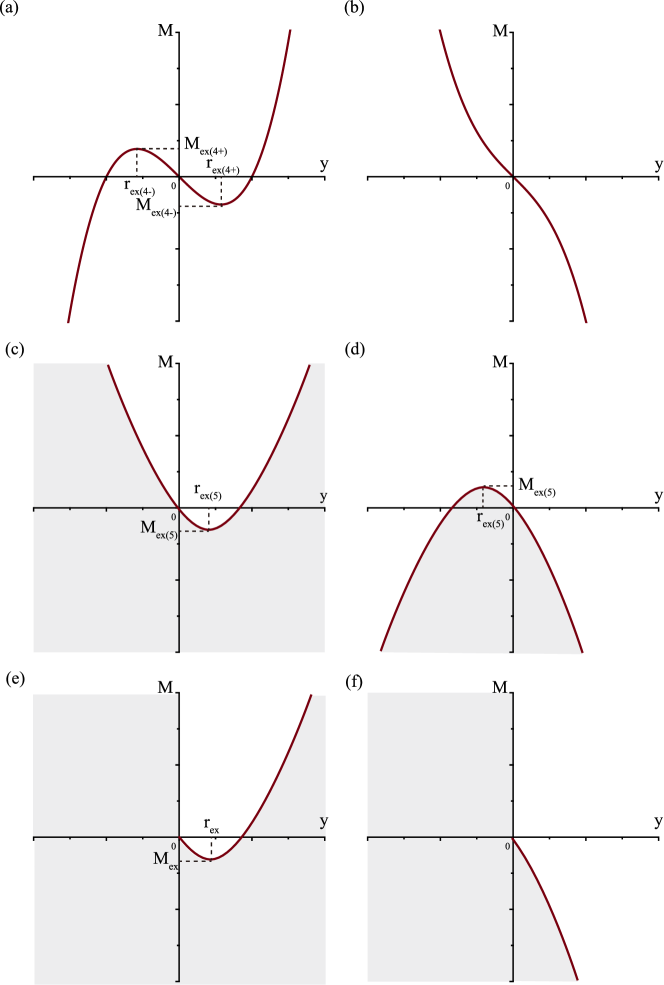
Figure 1: The forms of $M=M_{\rm s}(y)$ for (a) $n=4$ with $\zeta>0$, (b) $n=4$ with $\zeta<0$, (c) $n=5$ with $\zeta>0$, (d) $n=5$ with $\zeta<0$, (e) $n\geq 6$ with $\zeta>0$, and (f) $n\geq 6$ with $\zeta<0$. The metric (3.4) becomes complex and unphysical in shaded regions.

3.2 Parallelly propagated scalar curvature singularities

Next we show that $y=0$ and $y\to+\infty$ are parallelly propagated (p.p.) scalar curvature singularities for $n\geq 6$, which are defined by the fact that some component of the Riemann tensor in a parallelly propagated frame blows up [31].

For this purpose, we first derive components of the Riemann tensor $R_{(a)(b)(c)(d)}:=R_{\mu\nu\rho\sigma}E^{\mu}_{(a)}E^{\nu}_{(b)}E^{\rho}_{(c)}E^{\sigma}_{(d)}$ in a parallelly propagated orthonormal frame with basis vectors $E^{\mu}_{(a)}$, where $a=0,1,\cdots,n-1$, along an affinely parametrized and future-directed ingoing radial null geodesic $\gamma$ in the spacetime (3.4). A tangent vector $k^{\mu}$ of $\gamma$ satisfying $k_{\mu}k^{\mu}=0$ and $k^{\nu}\nabla_{\nu}k^{\mu}=0$ is given by

$$k^{\mu}\frac{\partial}{\partial x^{\mu}}=\frac{C}{\sqrt{2}}\biggl{(}\frac{\Pi}{y}\frac{\partial}{\partial t}-(n-3)\Pi^{(n-4)/(n-3)}\frac{\partial}{\partial y}\biggl{)},$$ (3.13)

where the sign of a constant $C$ is chosen in such a way that $k^{\mu}$ is future-directed. An orthogonal null vector to $k^{\mu}$ is given by

$$l^{\mu}\frac{\partial}{\partial x^{\mu}}=\frac{1}{\sqrt{2}C}\biggl{(}\frac{\partial}{\partial t}+\frac{(n-3)y}{\Pi^{1/(n-3)}}\frac{\partial}{\partial y}\biggl{)},$$ (3.14)

which satisfies $l_{\mu}l^{\mu}=0$ and $k_{\mu}l^{\mu}=-1$. Then we consider vectors $E^{\mu}_{(i)}~{}(i=2,3,\cdots,n-1)$ on ${\rm S}^{n-2}$ given by

$$E^{\mu}_{(i)}\frac{\partial}{\partial x^{\mu}}=\frac{1}{\Pi^{1/(n-3)}}e^{j}_{(i)}\frac{\partial}{\partial z^{j}},$$ (3.15)

which satisfy $g_{\mu\nu}E^{\mu}_{(i)}E^{\nu}_{(i)}=\delta_{(i)(j)}$, where $e^{j}_{(i)}$ are basis vectors on ${\rm S}^{n-2}$ satisfying

$$\gamma_{ij}e_{(k)}^{i}e_{(l)}^{j}=\delta_{(k)(l)}~{}\Leftrightarrow~{}\gamma^{ij}=\delta^{(k)(l)}e_{(k)}^{i}e_{(l)}^{j}.$$ (3.16)

Since $k^{\nu}\nabla_{\nu}l^{\mu}=0$ and $k^{\nu}\nabla_{\nu}E_{(i)}^{\mu}=0$ are satisfied, we identify $E^{\mu}_{(0)}\equiv k^{\mu}$ and $E^{\mu}_{(1)}\equiv l^{\mu}$ and then $E^{\mu}_{(a)}=\{k^{\mu},l^{\mu},E^{\mu}_{(i)}\}$ are basis vectors in a parallelly propagated orthonormal frame along $\gamma$. With the following expressions;

$${R}_{tyty}= \frac{-(n-3)y\Pi\Pi^{\prime\prime}+(n-2)\Pi^{\prime}(y\Pi^{\prime}-\Pi)}{2(n-3)\Pi^{3}},$$ (3.17)

$${R}_{titj}= -\frac{(n-3)y\Pi^{\prime}(y\Pi^{\prime}-\Pi)}{2\Pi^{2}}\gamma_{ij},$$ (3.18)

$${R}_{yiyj}= -\frac{2y\Pi\Pi^{\prime\prime}-\Pi^{\prime}(y\Pi^{\prime}-\Pi)}{2(n-3)y\Pi^{2(n-4)/(n-3)}}\gamma_{ij},$$ (3.19)

$${R}_{ijkl}= \Pi^{2/(n-3)}\left(k-y\Pi^{-1}{\Pi^{\prime}}^{2}\right)(\gamma_{ik}\gamma_{jl}-\gamma_{il}\gamma_{jk}),$$ (3.20)

non-zero components of $R_{(a)(b)(c)(d)}$ are computed to give

$$R_{(0)(1)(0)(1)}= -\frac{n-3}{2\Pi^{(n-1)/(n-3)}}\biggl{\{}(n-3)y\Pi\Pi^{\prime\prime}-(n-2)\Pi^{\prime}(y\Pi^{\prime}-\Pi)\biggl{\}},$$ (3.21)

$$R_{(0)(i)(0)(j)}= -\frac{1}{2}(n-3)C^{2}\Pi^{(n-5)/(n-3)}\Pi^{\prime\prime}\delta_{(i)(j)},$$ (3.22)

$$R_{(0)(i)(1)(j)}= R_{(1)(i)(0)(j)}=\frac{n-3}{2\Pi^{(n-1)/(n-3)}}\left\{y\Pi\Pi^{\prime\prime}-\Pi^{\prime}(y\Pi^{\prime}-\Pi)\right\}\delta_{(i)(j)},$$ (3.23)

$$R_{(1)(i)(1)(j)}= -\frac{(n-3)y^{2}\Pi^{\prime\prime}}{2C^{2}\Pi^{(n-1)/(n-3)}}\delta_{(i)(j)},$$ (3.24)

$$R_{(i)(j)(k)(l)}= \frac{1-y\Pi^{-1}{\Pi^{\prime}}^{2}}{\Pi^{2/(n-3)}}(\delta_{(i)(k)}\delta_{(j)(l)}-\delta_{(i)(l)}\delta_{(j)(k)}).$$ (3.25)

By the expression $\Pi^{\prime\prime}(y)=-2(n-1)\zeta y^{-(n-5)/(n-3)}/(n-3)^{2}$ and the finiteness of $\Pi(0)$ and $\Pi^{\prime}(0)$, $R_{(0)(i)(0)(j)}$ diverges as $y\to 0$ for $n\geq 6$, which shows that $y=0$ is a p.p. curvature singularity. Also, since $\lim_{y\to\infty}\Pi\simeq-\zeta y^{(n-1)/(n-3)}$ holds, we obtain $\lim_{y\to\infty}R_{(0)(i)(0)(j)}\propto y^{2(n-5)/(n-3)^{2}}$, which shows that $y\to\infty$ is a p.p. curvature singularity for $n\geq 6$, too. In contrast, $R_{(a)(b)(c)(d)}$ are finite as $y\to\pm\infty$ for $n=4$ and $5$.

3.3 Causal nature of boundaries

Here we clarify the causal nature of $y=0$, $y\to\pm\infty$, and $y=y_{\rm s}$ in the Penrose diagram. Causal nature of a hypersurface with constant $y(=y_{1})$ is determined by the two-dimensional Lorentzian portion with constant $z^{i}$ in the spacetime (3.4), of which conformally flat form is given by

$${\rm d}s_{2}^{2}=\frac{y}{\Pi(y)}(-{\rm d}t^{2}+{\rm d}y_{*}^{2}),$$ (3.26)

$$y_{*}:=\int^{y}\frac{\Pi({\bar{y}})^{1/(n-3)}}{(n-3){\bar{y}}}{\rm d}{\bar{y}}.$$ (3.27)

$y=y_{1}$ is non-null (null) if $y_{*}$ is finite (diverges) in the limit of $y\to y_{1}$.

Near $y=0$, we have

$$\Pi(y)\simeq\left\{\begin{array}[]{ll}2M&({\rm for}~{}M\neq 0)\\ y&({\rm for}~{}M=0)\end{array}\right.,$$ (3.30)

which shows that $\lim_{y\to 0}y_{*}$ blows up for $M\neq 0$ and it is finite for $M=0$. Hence, $y=0$ is null and timelike for $M\neq 0$ and $M=0$, respectively. Next, as $y\to\pm\infty$, we obtain $\lim_{y\to\pm\infty}y_{*}\propto y^{(n-1)/(n-3)^{2}}$, which blows up for any $n(\geq 4)$. Therefore, $y\to\pm\infty$ are null. Lastly, near $y=y_{\rm s}(\neq 0)$, we have $\Pi(y_{\rm s})\simeq\Pi_{1}(y-y_{\rm s})^{b}$, where $\Pi_{1}$ is a non-zero constant and $b$ is given by

$$b=\left\{\begin{array}[]{ll}2&({\rm at~{}an~{}extremum~{}of}~{}M=M_{\rm s}(y))\\ 1&({\rm otherwise})\end{array}\right..$$ (3.33)

Since $y_{*}$ is finite as $y\to y_{\rm s}$ both for $b=1$ and $2$, the singularity at $y=y_{\rm s}$ is non-null.

Let us also check extendibility of these boundaries. For this purpose, we need to study affinely parametrized radial null geodesics. Since the spacetime (3.4) admits a hypersurface-orthogonal Killing vector $\xi^{\mu}\partial/\partial x^{\mu}=\partial/\partial t$, there is a conserved quantity $E:=-\xi_{\mu}k^{\mu}$ along a geodesic with its tangent vector $k^{\mu}$. A future-directed radial null geodesic $\gamma$ is described by $x^{\mu}=(t(\lambda),y(\lambda),0,\cdots,0)$, where $\lambda$ is an affine parameter along $\gamma$. Then, by the expression $E=y\Pi^{-1}({\rm d}t/{\rm d}\lambda)$ and the null condition ${\rm d}s^{2}=0$, we obtain

$$\frac{{\rm d}y}{{\rm d}\lambda}=\pm(n-3)|E|\Pi^{(n-4)/(n-3)},$$ (3.34)

which is integrated to give

$$\pm(n-3)|E|(\lambda-\lambda_{0})=\int^{y}\Pi({\bar{y}})^{-(n-4)/(n-3)}{\rm d}{\bar{y}},$$ (3.35)

where $\lambda_{0}$ is an integration constant and the plus (minus) sign corresponds to outgoing (ingoing) $\gamma$. Then, $y=y_{1}$ is null infinity if $\lambda$ diverges as $y\to y_{1}$. If $y\to y_{1}$ is regular and corresponds to a finite value of $\lambda$, the spacetime is extendible beyond $y=y_{1}$.

First, $y=0$ is not null infinity because the expression (3.30) shows that $\lambda$ is finite there. Next, as $y\to\pm\infty$, the right-hand side of Eq. (3.35) behaves as

$$\int^{y}\Pi({\bar{y}})^{-(n-4)/(n-3)}{\rm d}{\bar{y}}\simeq(-\zeta)^{-(n-4)/(n-3)}\int^{y}{\bar{y}}^{-(n-1)(n-4)/(n-3)^{2}}{\rm d}{\bar{y}}.$$ (3.36)

Since Eq. (3.36) diverges for $n=4$ and $5$ and remains finite for $n\geq 6$, $y\to\pm\infty$ are null infinities for $n=4$ and $5$, while a p.p. curvature singularity $y\to+\infty$ for $n\geq 6$ is not null infinity. Lastly, near $y=y_{\rm s}$, we have $\Pi(y_{\rm s})\simeq\Pi_{1}(y-y_{\rm s})^{b}$ with $b$ given by Eq. (3.33). It shows that $\lambda$ diverges as $y\to y_{\rm s}$ only for $b=2$ with $n\geq 5$. Therefore, the singularity $y=y_{\rm s}$ is not null infinity except for the case where $y=y_{\rm s}$ is an extremum of $M=M_{\rm s}(y)$ for $n\geq 5$.

Based on these results, one can draw the Penrose diagrams of the Semiz class-I solution with $k=1$ depending on $M$, $\zeta$, and $n$, as summarized in Tables 1, 2, and 3 for $n=4$, $n=5$, and $n\geq 6$, respectively.

Table 1: Penrose diagrams of the Semiz class-I solution with $k=1$ and $n=4$. If $M=M_{\rm s}(y)$ admits more than one real solution for a given $M$, they are represented as $y=y_{\rm s(i)}~{}(i=1,2,\cdots)$ satisfying $y_{\rm s(i)}<y_{\rm s(i+1)}$.

$\zeta$	$M$	Domain of $y$	Diagram in Fig. 2
$\zeta>0$	$M>M_{\rm ex(4+)}$	$y_{\rm s}<y<\infty$	C1
		$-\infty<y<y_{\rm s}$	NS7
	$M=M_{\rm ex(4+)}$	$y_{\rm s(2)}<y<\infty$	C1
	(then $y_{\rm s(1)}=y_{\rm ex(4-)}$)	$y_{\rm ex(4-)}<y<y_{\rm s(2)}$	NS6
		$-\infty<y<y_{\rm ex(4-)}$	C1
	$0<M<M_{\rm ex(4+)}$	$y_{\rm s(3)}<y<\infty$	C1
		$y_{\rm s(2)}<y<y_{\rm s(3)}$	NS6
		$y_{\rm s(1)}<y<y_{\rm s(2)}$	NS5
		$-\infty<y<y_{\rm s(1)}$	C1
	$M=0$	$y_{\rm s(3)}<y<\infty$	C1
	(then $y_{\rm s(2)}=0$)	$0<y<y_{\rm s(3)}$	NS4
		$y_{\rm s(1)}<y<0$	NS4
		$-\infty<y<y_{\rm s(1)}$	C1
	$M_{\rm ex(4-)}<M<0$	$y_{\rm s(3)}<y<\infty$	C1
		$y_{\rm s(2)}<y<y_{\rm s(3)}$	NS5
		$y_{\rm s(1)}<y<y_{\rm s(2)}$	NS6
		$-\infty<y<y_{\rm s(1)}$	C1
	$M=M_{\rm ex(4-)}$	$y_{\rm ex(4+)}<y<\infty$	C1
	(then $y_{\rm s(2)}=y_{\rm ex(4+)}$)	$y_{\rm s(1)}<y<y_{\rm ex(4+)}$	NS6
		$-\infty<y<y_{\rm s(1)}$	C1
	$M<M_{\rm ex(4-)}$	$y_{\rm s}<y<\infty$	NS7
		$-\infty<y<y_{\rm s}$	C1
$\zeta<0$	$M>0$	$y_{\rm s}<y<\infty$	BH1
		$-\infty<y<y_{\rm s}$	NS1
	$M=0$	$0\leq y<\infty$	R
		$-\infty<y\leq 0$	R
	$M<0$	$y_{\rm s}<y<\infty$	NS1
		$-\infty<y<y_{\rm s}$	BH1

Table 2: Penrose diagrams of the Semiz class-I solution with $k=1$ and $n=5$. See the caption of Table 1.

$\zeta$	$M$	Domain of $y$	Diagram in Fig. 2
$\zeta>0$	$M>0$	$y_{\rm s(1)}<y<y_{\rm s(2)}$	NS6
	$M=0$ (then $y_{\rm s(1)}=0$)	$0\leq y<y_{\rm s(2)}$	NS4
	$M_{\rm ex(5)}<M<0$	$y_{\rm s(1)}<y<y_{\rm s(2)}$	NS5
$\zeta<0$	$M>M_{\rm ex(5)}$	$-\infty<y<\infty$	BH3
	$M=M_{\rm ex(5)}$	$r_{\rm ex(5)}<y<\infty$	BH2
		$-\infty<y<r_{\rm ex(5)}$	C2
	$0<M<M_{\rm ex(5)}$	$y_{\rm s(2)}<y<\infty$	BH1
		$-\infty<y<y_{\rm s(1)}$	C1
	$M=0$	$0\leq y<\infty$	R
	(then $y_{\rm s(2)}=0$)	$-\infty<y<y_{\rm s(1)}$	C1
	$M<0$	$y_{\rm s(2)}<y<\infty$	NS1
		$-\infty<y<y_{\rm s(1)}$	C1

Table 3: Penrose diagrams of the Semiz class-I solution with $k=1$ and $n\geq 6$. See the caption of Table 1.

$\zeta$	$M$	Domain of $y$	Diagram in Fig. 2
$\zeta>0$	$M>0$	$0<y<y_{\rm s}$	NS8
	$M=0$ (then $y_{\rm s(1)}=0$)	$0\leq y<y_{\rm s(2)}$	NS4
	$M_{\rm ex}<M<0$	$y_{\rm s(1)}<y<y_{\rm s(2)}$	NS5
$\zeta<0$	$M>0$	$0<y<\infty$	NS9
	$M=0$	$0\leq y<\infty$	NS3
	$M<0$	$y_{\rm s}<y<\infty$	NS2

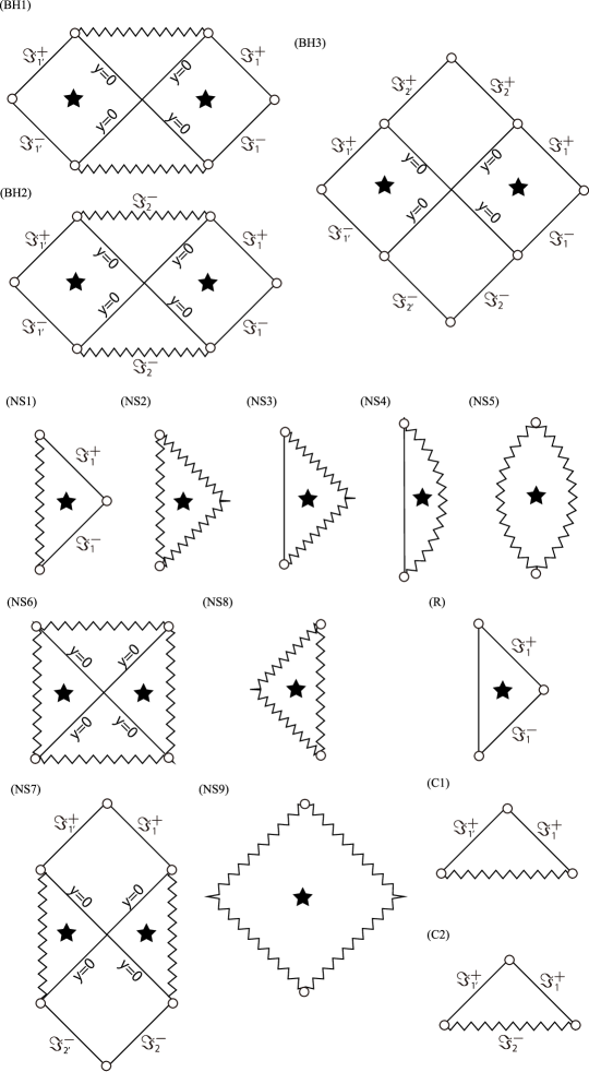
Figure 2: Possible Penrose diagrams of the Semiz class-I solution with $k=1$ and $\zeta\neq 0$. A zig-zag line or curve is a curvature singularity and the spacetime is static in a region with a black star. $\Im^{+(-)}$ stands for a future (past) null infinity and its indices are to distinguish different infinities. BH, NS, R, and C stand for “Black Hole”, “Naked Singularity”, “Regular”, and “Cosmological”, respectively. Time-reversal (upside-down) diagrams are also possible for (C1) and (C2).

3.4 Regular Killing horizon for $n=4$ and $5$

The spacetime (3.4) admits a hypersurface orthogonal Killing vector $\xi^{\mu}(\partial/\partial x^{\mu})=\partial/\partial t$, of which squared norm is $\xi_{\mu}\xi^{\mu}=-y/\Pi(y)$, so that $\xi^{\mu}$ is timelike (spacelike) in a region where $y/\Pi>(<)0$ holds. A Killing horizon associated with $\xi^{\mu}$ is a regular null hypersurface $y=0$ for $M\neq 0$. For $M=0$, we have $\xi_{\mu}\xi^{\mu}=-(1-\zeta y^{2/(n-3)})^{-1}$, so that $y=0$ is not a Killing horizon but a regular center $r=0$ as shown in the metric (3.11). Therefore, we will focus on the case with $M\neq 0$ (and $\zeta\neq 0$).

In terms of the null coordinate defined by

$$v:=t+\int\frac{\Pi(y)^{1/(n-3)}}{(n-3)y}{\rm d}y,$$ (3.37)

the metric (3.4) becomes

$${\rm d}s^{2}=-\frac{y}{\Pi(y)}{\rm d}v^{2}+\frac{2}{(n-3)\Pi(y)^{(n-4)/(n-3)}}{\rm d}v{\rm d}y+\Pi(y)^{2/(n-3)}\gamma_{ij}{\rm d}z^{i}{\rm d}z^{j}.$$ (3.38)

In terms of the coordinate $r$, this metric becomes

$${\rm d}s^{2}=-f(r){\rm d}v^{2}+\frac{2}{h(r)^{(n-4)/(n-3)}}{\rm d}v{\rm d}r+r^{2}h(r)^{2/(n-3)}\gamma_{ij}{\rm d}z^{i}{\rm d}z^{j}$$ (3.39)

where $f(r)$ and $h(r)$ are defined by Eqs. (3.2) and (3.3), respectively. Both of these metrics and their inverses are $C^{\infty}$ at $y=0$ and $r^{n-3}=2M$ for $n=4$ and $5$ and hence it is a Killing horizon. In contrast, they are $C^{1}$ at a p.p. curvature singularity $y=0$ for $n\geq 6$. In this subsection, we study the properties of $y=0$ in more detail.

3.4.1 Matter field on and off the Killing horizon

Here we study the matter field of the Semiz class-I solution (3.4) and discuss the standard energy conditions. The standard energy conditions consist of the null energy condition (NEC), weak energy condition (WEC), dominant energy condition (DEC), and strong energy condition (SEC). (See section 2 in [16].) It is emphasized that, although the matter field in a static region is a perfect fluid (2.2), it is not the case in different regions.

In fact, in the region of $y\neq 0$, the matter field is described by the following anisotropic fluid in general;

$${T}_{\mu\nu}=(\mu+p_{2})u_{\mu}u_{\nu}+(p_{1}-p_{2})s_{\mu}s_{\nu}+p_{2}g_{\mu\nu},$$ (3.40)

where $\mu$, $p_{1}$, and $p_{2}$ are energy density, radial pressure, and tangential pressure of the fluid, respectively, and $u_{\mu}u^{\mu}=-1$, $s_{\mu}s^{\mu}=1$, and $u_{\mu}s^{\mu}=0$ hold. This matter field becomes a perfect fluid if $p_{1}=p_{2}\equiv p$ is satisfied. Equivalent expressions of the standard energy conditions for an anisotropic fluid (3.40) are given by

$$\mbox{NEC}: ~{}~{}\mu+p_{i}\geq 0~{}(i=1,2),$$ (3.41)

$$\mbox{WEC}: ~{}~{}\mu\geq 0\mbox{~{}in addition to NEC},$$ (3.42)

$$\mbox{DEC}: ~{}~{}\mu-p_{i}\geq 0~{}(i=1,2)\mbox{~{}in addition to WEC},$$ (3.43)

$$\mbox{SEC}: ~{}~{}(n-3)\mu+p_{1}+(n-2)p_{2}\geq 0\mbox{~{}in addition to NEC}.$$ (3.44)

(See section 3.1 in [16].)

Non-zero components of the energy-momentum tensor for the Semiz class-I solution (3.4) are

$$T^{t}_{~{}t}=-\rho,\qquad T^{y}_{~{}y}=-\frac{n-3}{n+1}\rho,\qquad T^{i}_{~{}j}=-\frac{n-3}{n+1}\rho\delta^{i}_{~{}j},$$ (3.45)

where $\rho$ is given by Eq. (3.5). In a static region given by $y\Pi>0$ for $n=4$ and $y>0$ with $\Pi>0$ for $n\geq 5$, where $y$ is a spacelike coordinate, this matter field is described by Eq. (3.40) with

$$\mu=\rho,\qquad p_{1}=p_{2}=-\frac{n-3}{n+1}\rho,$$ (3.46)

$$u^{\mu}\frac{\partial}{\partial x^{\mu}}=\sqrt{\frac{\Pi}{y}}\frac{\partial}{\partial t},$$ (3.47)

which is certainly a perfect fluid (2.2) obeying $p=-(n-3)\rho/(n+1)$. In this case, all the standard energy conditions are satisfied (violated) for $\zeta>(<)0$.

On the other hand, in a dynamical region given by $y\Pi<0$ for $n=4$ and $y<0$ with $\Pi>0$ for $n\geq 5$, where $y$ is a timelike coordinate, the matter field is an anisotropic fluid (3.40) with

$$\mu=\frac{n-3}{n+1}\rho,\qquad p_{1}=-\rho,\qquad p_{2}=-\frac{n-3}{n+1}\rho,$$ (3.48)

$$u^{\mu}\frac{\partial}{\partial x^{\mu}}=\sqrt{-\frac{(n-3)^{2}y}{\Pi^{-(n-5)/(n-3)}}}\frac{\partial}{\partial y},\qquad s^{\mu}\frac{\partial}{\partial x^{\mu}}=\sqrt{-\frac{\Pi}{y}}\frac{\partial}{\partial t}.$$ (3.49)

By the following expressions

$$\mu+p_{1}=-\frac{4}{n+1}\rho,\quad\mu+p_{2}=0,$$ (3.50)

$$\mu-p_{1}=\frac{2(n-1)}{n+1}\rho,\quad\mu-p_{2}=\frac{2(n-3)}{n+1}\rho,$$ (3.51)

$$(n-3)\mu+p_{1}+(n-2)p_{2}=-\frac{2(n-1)}{n+1}\rho$$ (3.52)

and Eqs (3.41)–(3.44), all the standard energy conditions are violated for $\zeta>0$, while the NEC and SEC are satisfied for $\zeta<0$.

In contrast, a matter field on the Killing horizon $y=0$ for $n=4$ and $5$ is very non-trivial because $y=0$ is a coordinate singularity in the metric (3.4). We identify the matter field on the Killing horizon $y=0$ with the regular metric (3.38) at $y=0$. Non-zero components of the Einstein tensor in this coordinate system are given by

$$G^{v}_{~{}v}= -\frac{(n-1)(n+1)(n-2)}{2(n-3)}\zeta y^{2/(n-3)}\Pi^{-2/(n-3)},$$ (3.53)

$$G^{v}_{~{}y}= \frac{2(n-1)(n-2)}{(n-3)^{2}}\zeta y^{-(n-5)/(n-3)}\Pi^{-1/(n-3)},$$ (3.54)

$$G^{y}_{~{}v}= 0,$$ (3.55)

$$G^{y}_{~{}y}= -\frac{1}{2}(n-1)(n-2)\zeta y^{2/(n-3)}\Pi^{-2/(n-3)},$$ (3.56)

$$G^{i}_{~{}j}= -\frac{1}{2}(n-1)(n-2)\zeta y^{2/(n-3)}\Pi^{-2/(n-3)}\delta^{i}_{~{}j}.$$ (3.57)

For $M\neq 0$, we obtain

$$G^{v}_{~{}v}|_{y=0}= G^{y}_{~{}v}|_{y=0}=G^{y}_{~{}y}|_{y=0}=G^{i}_{~{}j}|_{y=0}=0,$$ (3.58)

$$G^{v}_{~{}y}|_{y=0}= \left\{\begin{array}[]{ll}0&(n=4)\\ 24\zeta/\sqrt{2M}&(n=5)\\ \infty&(n\geq 6)\\ \end{array}\right..$$ (3.62)

Therefore, a matter field is absent on the Killing horizon for $n=4$, as shown in [32]. In contrast, divergence of $\lim_{y\to 0}G^{v}_{~{}y}$ for $n\geq 6$ suggests that $y=0$ is a p.p. curvature singularity.

For $n=5$, the matter field at $y=0$ is a null dust fluid, of which energy-momentum tensor is given by

$$T_{\mu\nu}|_{y=0}=\Omega l_{\mu}l_{\nu},\qquad l^{\mu}\frac{\partial}{\partial x^{\mu}}=l^{0}\frac{\partial}{\partial v},$$ (3.63)

where $\Omega$ is the energy density and $l^{\mu}$ is a null vector satisfying $\Omega(l^{0})^{2}=48\zeta/\kappa_{5}$. This null dust fluid satisfies (violates) all the standard energy conditions for $\zeta>(<)0$. (See section 4.2 in [16].) If we assume that the null dust moves geodesically and is parametrized by an affine parameter $\lambda$, $\Omega$ and $l^{0}$ are given by

$$\Omega=\frac{24\zeta}{\kappa_{5}M}(\lambda-\lambda_{0})^{2},\qquad l^{0}=\frac{\sqrt{2M}}{\lambda-\lambda_{0}},$$ (3.64)

where $\lambda_{0}$ is an integration constant. (See Appendix B.) In this case, $\Omega$ converges to zero in the limit $\lambda\to\lambda_{0}$ corresponding to a bifurcation $(n-2)$-sphere $v\to-\infty$, on which the Killing vector generating staticity vanishes [33]. Our results are summarized in Table 4.

Table 4: The standard energy conditions that the mater field of the Semiz class-I solution with $k=1$ satisfies in different domains of $y$. $\Pi>0$ is required for $n\geq 5$ and $y>0$ is required for $n\geq 6$ in addition.

Domain of $y$	$n$	Matter	$\zeta>0$	$\zeta<0$
$y\Pi>0$	$n\geq 4$	Perfect fluid	All	None
$y=0$	$n=4$	Vacuum	All	All
	$n=5$	Null dust	All	None
$y\Pi<0$	$n=4,5$	Anisotropic fluid	None	NEC & SEC

3.4.2 Regular attachment to Schwarzschild-Tangherlini spacetime

Lastly, we show that, for $n=4$ and $5$, two Semiz class-I spacetimes with the same $M$ but different $\zeta$ can be attached at the Killing horizon $y=0$ in a regular manner. In other words, they can be attached without a massive lightlike thin-shell, which is a localized matter field at $y=0$ described by the delta-function. As a special case, a Semiz class-I spacetime with $M>0$ can be attached to the Schwarzschild-Tangherlini vacuum black-hole spacetime at $y=0$. To prove this, we will use the junction conditions at a null hypersurface developed in [34, 35], (See also Section 3.11 in the textbook [36].) Attachment of spacetimes at a Killing horizon has recently been studied in a more general setup in [37].

For our purpose, we use the Semiz class-I metric (3.38) with the null coordinate $v$. Let $\Sigma$ be a Killing horizon, which is a null hypersurface given by $y=0$. The parametric equations $x^{\mu}=x^{\mu}({\eta},\theta^{i})$ describing $\Sigma$ are $v=\eta$, $y=0$, and $\theta^{i}=z^{i}$. The line element on $\Sigma$ is $(n-2)$-dimensional and given by

$${\rm d}s_{\Sigma}^{2}=h_{ab}{\rm d}w^{a}{\rm d}w^{b}=(2M)^{2/(n-3)}\gamma_{ij}{\rm d}z^{i}{\rm d}z^{j}(=\sigma_{ij}{\rm d}\theta^{i}{\rm d}\theta^{j}),$$ (3.65)

where $w^{a}=(\eta,z^{i})$ is a set of coordinates on $\Sigma$. Using them, we obtain the tangent vectors of $\Sigma$ defined by $e^{\mu}_{a}:=\partial x^{\mu}/\partial y^{a}$ as

$$e^{\mu}_{\eta}\frac{\partial}{\partial x^{\mu}}=\frac{\partial}{\partial v},\qquad e^{\mu}_{i}\frac{\partial}{\partial x^{\mu}}=\frac{\partial}{\partial z^{i}}.$$ (3.66)

An auxiliary null vector $N^{\mu}$ given by

$$N^{\mu}\frac{\partial}{\partial x^{\mu}}=-(n-3)\Pi(y)^{(n-4)/(n-3)}\frac{\partial}{\partial y}$$ (3.67)

completes the basis. The expression $N_{\mu}{\rm d}x^{\mu}=-{\rm d}v$ shows $N_{\mu}N^{\mu}=0$, $N_{\mu}e^{\mu}_{\eta}=-1$, and $N_{\mu}e^{\mu}_{i}=0$. The completeness relation of the basis on $\Sigma$ is given as

$$g^{\mu\nu}|_{\Sigma}=-k^{\mu}N^{\nu}-N^{\mu}k^{\nu}+\sigma^{ij}e^{\mu}_{i}e^{\nu}_{j},$$ (3.68)

where $k^{\mu}\equiv e^{\mu}_{\eta}$ and $\sigma^{ij}$ is the inverse of $\sigma_{ij}$.

Since $\sigma_{ij}$, $e^{\mu}_{a}$, and $N^{\mu}$ do not include $\zeta$ on $\Sigma$, $[e^{\mu}_{a}]=[N^{\mu}]=[\sigma_{ij}]=0$ are realized on $\Sigma$ when two Semiz class-I spacetimes with the same $M$ but different $\zeta$ are attached at $\Sigma$. Here $[X]$ is the difference of $X$ evaluated on the two sides of $\Sigma$. As a result, if the transverse derivative of the metric is continuous at $\Sigma$, a $C^{1}$ regular attachment of two spacetimes at $\Sigma$ is achieved. In other words, there is no massive lightlike thin-shell at $\Sigma$ if $N^{\rho}[\partial_{\rho}g_{\mu\nu}]=0$ holds there. This condition is equivalent to $[C_{ab}]=0$, where $C_{ab}:=(\nabla_{\nu}N_{\mu})e^{\mu}_{a}e^{\nu}_{b}$ is the transverse curvature at $\Sigma$.

In the present case, nonvanishing component of $C_{ab}$ of $\Sigma$ are given by

$$\begin{aligned} &C_{\eta\eta}=\Gamma^{v}_{vv}|_{y=0}=\frac{n-3}{2(2M)^{1/(n-3)}},\\ &C_{ij}=\Gamma^{v}_{ij}|_{y=0}=-(2M)^{1/(n-3)}\gamma_{ij}.\end{aligned}$$ (3.69)

Since Eq. (3.69) is characterized only by $M$ and does not contain $\zeta$, $[C_{ab}]=0$ is realized if one attaches two Semiz class-I spacetimes with the same $M$ but different values of $\zeta$ at the Killing horizon $y=0$.

As a special case, one can attach the Semiz class-I solution with $M>0$ in a regular manner to the Schwarzschild-Tangherlini black-hole spacetime described by Eq. (3.38) with $\zeta=0$ and the same $M$. In this construction, we assume that $y=0$ is a part of the Schwarzschild-Tangherlini spacetime so that a matter field is absent at the Killing horizon. The Penrose diagrams of the resulting spacetime and the energy conditions that are fulfilled depending on the parameters are summarized in Table 5. Figure 3(a) describes a perfect fluid hovering outside the Schwarzschild-Tangherlini black hole. Figures 3(b), (c), and (d) describe a Schwarzschild-Tangherlini black hole with its interior replaced by the Semiz class-I spacetime. In particular, Fig. 3(b) describes a non-singular black hole of the big-bounce type. The difference between Figs. 3(c) and (d) is the fact that the singularity of the latter is null infinity.

Table 5: Four- and five-dimensional asymptotically (locally) flat black holes constructed by attaching the spherically symmetric Semiz class-I solution with $M>0$ to the Schwarzschild-Tangherlini vacuum solution with the same $M$ at the Killing horizon $y=0$. The matter in the Semiz class-I region with $y>0$ and $y<0$ is a perfect fluid and an anisotropic fluid, respectively.

$n$	$y<0$	$y>0$	Diagram in Fig. 3	Energy conditions
$4$	Schwarzschild	Semiz class-I ($\zeta<0$)	(a) for $M>0$	None
	Semiz class-I ($\zeta<0$)	Schwarzschild	(c) for $M>0$	NEC & SEC
	Semiz class-I ($\zeta>0$)	Schwarzschild	(c) for $0<M\leq M_{\rm ex(4+)}$	None
			(b) for $M>M_{\rm ex(4+)}$
$5$	Tangherlini	Semiz class-I ($\zeta<0$)	(a) for $M>0$	None
	Semiz class-I ($\zeta<0$)	Tangherlini	(c) for $0<M<M_{\rm ex(5)}$	NEC & SEC
			(d) for $M=M_{\rm ex(5)}$
			(b) for $M>M_{\rm ex(5)}$
	Semiz class-I ($\zeta>0$)	Tangherlini	(c) for $M>0$	None

We note that the configuration of Fig. 3(a) does not contradict to the theorems by Shiromizu, Yamada, and Yoshino [38] for $n=4$ and by Rogatko [39] for arbitrary $n(\geq 4)$, which prohibit any static configuration of a star composed of a perfect fluid in an asymptotically flat black-hole spacetime. This is because the configuration of a static perfect fluid in Fig. 3(a) is not a star. Furthermore, it violates the dominant energy condition and the spacetime is not asymptotically flat but asymptotically locally flat, which are assumptions of the theorems in [38, 39].

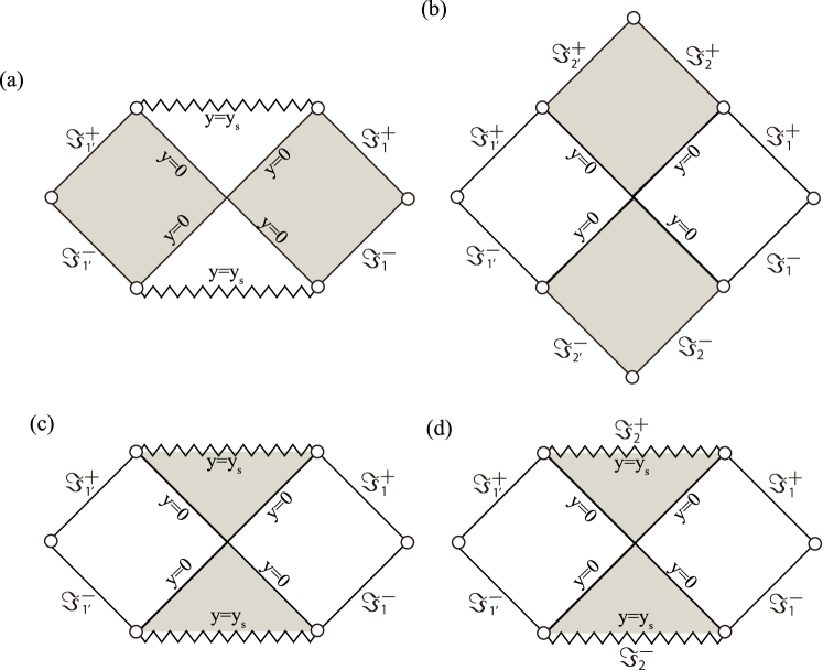
Figure 3: Possible Penrose diagrams of an asymptotically (locally) flat black hole in four and five dimensions constructed by attaching the Semiz class-I solution with $k=1$ to the Schwarzschild-Tangherlini solution at the Killing horizon $y=0$ (which is $r^{n-3}=2M$). Shaded regions are described by the Semiz class-I solution. See the caption of Fig. 2.

4 Summary and concluding remarks

We summarize the main results of the present paper.

• We have obtained the general $n(\geq 4)$-dimensional static solution with an $(n-2)$-dimensional Einstein base manifold for a perfect fluid obeying a linear equation of state $p=-(n-3)\rho/(n+1)$, which is a generalization of Semiz’s four-dimensional general solution with spherical symmetry [19] and consists of two classes of solutions.

• The class-I and class-II solutions are dual to the topological Schwarzschild-Tangherlini-(A)dS solution and one of the $\Lambda$-vacuum direct-product solutions, respectively, through the $n(\geq 4)$-dimensional Buchdahl transformation in Proposition 1.

• The spherically symmetric class-I solution (3.1), characterized by two parameters $M$ and $\zeta$, is asymptotically locally flat as $r\to\pm\infty$. While the metric and its inverse of the solution are $C^{\infty}$ at the Killing horizon $r^{n-3}=2M$ for $n=4$ and $5$, they are $C^{1}$ for $n\geq 6$ and then the Killing horizon turns to be a p.p. curvature singularity. The matter field on the Killing horizon is absent for $n=4$ and a null dust fluid for $n=5$. For $n=4$ and $5$, two spherically symmetric class-I spacetimes with the same $M$ but different $\zeta$ can be attached at the Killing horizon in a regular manner, namely without a lightlike massive thin-shell.

• As a special case, a spherically symmetric class-I spacetime with $M>0$ and $\zeta\neq 0$ can be regularly attached at the Killing horizon to the Schwarzschild-Tangherlini vacuum black hole with the same $M$, which allows totally new configurations of an asymptotically (locally) flat black hole, as shown in Table 5.

In the last configuration of a black hole, as shown in Table 5, all the standard energy conditions are violated when the static perfect fluid hovers outside a vacuum black hole. On the other hand, the null and strong energy conditions can be satisfied when the dynamical region inside the event horizon of a vacuum black hole is replaced by the Semiz class-I solution with $\zeta<0$. In this case, the spacetime always involves a spacelike singularity inside the horizon for $n=4$ but it describes a non-singular black hole of the big-bounce type for $n=5$ if $M$ is larger than a critical value $M_{\rm ex(5)}:=-1/(8\zeta)(>0)$. It should be emphasized that the exterior of this black hole is dynamically stable against linear perturbations because it is exactly the Schwarzschild-Tangherlini spacetime [40, 41]. For the same reason, this black hole in four dimensions ($n=4$) cannot be distinguished from the Schwarzschild black hole by observations. However, it is of course highly non-trivial how these new configurations of a black hole can be formed from, for example, gravitational collapse.

We have shown that, in the Semiz class-I solution for $k=1$, the metric on the Killing horizon is $C^{\infty}$ for $n=4$ and $5$, but it becomes $C^{1}$ for $n\geq 6$ and then the Killing horizon turns to be a p.p. curvature singularity. This is similar to the property of the $n(\geq 4)$-dimensional Majumdar-Papapetrou solution in the Einstein-Maxwell system [42, 43, 44]. It describes a multi black hole with the $C^{\infty}$ metric at the extreme Killing horizon for $n=4$ [45], but the metric becomes $C^{2}$ at the horizon for $n=5$ and the Killing horizon turns to be a p.p. curvature singularity for $n\geq 6$ [46]. (See also [47].) Those examples show that the problem of differentiability of a Killing horizon in $n$-dimensional solutions with matter fields is an interesting problem worth pursuing. Although a simple method to prove non-smoothness of a black-hole horizon has been proposed in [48], we still don’t know the answer for static and spherically symmetric perfect-fluid solutions obeying a more general equation of state. We leave this problem for further research.

Acknowledgements

The author thanks Tetsuya Shiromizu for communications about the result in [38] and Tomohiro Harada for discussions on junction conditions.

Appendix A Generalized Tolman-VI solution for $p=\chi\rho$

The Einstein equations (2.1) with a perfect fluid (2.2) obeying an equation of state $p=\chi\rho$ admits the following solution for $n\geq 4$ with $k\neq 0$:

$$\begin{aligned} &{\rm d}s^{2}=-r^{4\chi/(1+\chi)}{\rm d}t^{2}+\frac{(n-3)(1+\chi^{2})+2(n-1)\chi}{k(n-3)(1+\chi)^{2}}{\rm d}r^{2}+r^{2}\gamma_{ij}{\rm d}z^{i}{\rm d}z^{j},\\ &u^{\mu}\frac{\partial}{\partial x^{\mu}}=r^{-2\chi/(1+\chi)}\frac{\partial}{\partial t},\qquad\rho=\frac{1}{\chi}p=\frac{2(n-2)(n-3)k\chi}{\kappa_{n}[(n-3)(1+\chi^{2})+2(n-1)\chi]r^{2}}.\end{aligned}$$ (A.1)

The solution (A.1) with $n=4$ with $k=1$ is identical to the Tolman-VI solution with $B=0$ [2] and a particular case of the self-similar (homothetic) static solution obtained by Henriksen and Wesson [49].

For the Lorentzian signature, $k[(n-3)(1+\chi^{2})+2(n-1)\chi]>0$ is required, which is equivalent to $\chi<\chi_{-}$ and $\chi>\chi_{+}$ for $k=1$ and $\chi_{-}<\chi<\chi_{+}$ for $k=-1$, where

$$\chi_{\pm}=\chi_{\pm}(n):=\frac{-(n-1)\pm 2\sqrt{n-2}}{n-3}(<0).$$ (A.2)

$\chi_{+}(n)$ is a monotonically decreasing function and satisfies $\chi_{+}(4)=-3+2\sqrt{2}\simeq-0.17$ and $\lim_{n\to\infty}\chi_{+}(n)=-1$. $\chi_{-}(n)$ is a monotonically increasing function and satisfies $\chi_{-}(4)=-3-2\sqrt{2}\simeq-5.8$ and $\lim_{n\to\infty}\chi_{-}(n)=-1$. Therefore, $-1<\chi_{+}\leq-3+2\sqrt{2}$ and $-3-2\sqrt{2}\leq\chi_{-}<-1$ hold for $n\geq 4$.

It is noted that the solution (A.1) is invariant under the Buchdahl transformation in Proposition 1 with $\Omega^{-2}=r^{4\chi/(1+\chi)}$. The metric of the generated solution is

$${\rm d}s^{2}= -r^{-4\chi/(1+\chi)}{\rm d}t^{2}+\frac{(n-3)(1+\chi^{2})+2(n-1)\chi}{k(n-3)(1+\chi)^{2}}r^{8\chi/[(n-3)(1+\chi)]}{\rm d}r^{2}$$

$$~{}~{}~{}~{}~{}~{}~{}~{}~{}~{}~{}~{}~{}~{}+r^{2[(n-3)+(n+1)\chi]/[(n-3)(1+\chi)]}\gamma_{ij}{\rm d}z^{i}{\rm d}z^{j},$$ (A.3)

which becomes

$${\rm d}s^{2}=-{\bar{r}}^{4{\bar{\chi}}/(1+{\bar{\chi}})}{\rm d}t^{2}+\frac{(n-3)(1+{\bar{\chi}}^{2})+2(n-1){\bar{\chi}}}{k(n-3)(1+{\bar{\chi}})^{2}}{\rm d}{\bar{r}}^{2}+{\bar{r}}^{2}\gamma_{ij}{\rm d}z^{i}{\rm d}z^{j}$$ (A.4)

by the following coordinate transformation and a redefinition of the parameter:

$${\bar{r}}:= r^{[(n-3)+(n+1)\chi]/[(n-3)(1+\chi)]},$$ (A.5)

$${\bar{\chi}}:= -\frac{(n-3)\chi}{(n-3)+2(n-1)\chi}.$$ (A.6)

Appendix B Radial null geodesics confined on the Killing horizon $y=0$

Consider a future-directed radial null geodesic $\gamma$ in the Semiz class-I spacetime with the metric (3.38), which is represented by $x^{\mu}=(v(\lambda),y(\lambda),0,\cdots,0)$ with its tangent vector $l^{\mu}=({\dot{v}},{\dot{y}},0,\cdots,0)$, where $\lambda$ is an affine parameter along $\gamma$ and a dot denotes differentiation with respect to $\lambda$. Null geodesic equations $l^{\nu}\nabla_{\nu}l^{\mu}=0$ along $\gamma$ are written as

$$0= {\ddot{v}}-\frac{n-3}{2}\Pi^{-1/(n-3)}(y\Pi^{-1}\Pi^{\prime}-1){\dot{v}}^{2},$$ (B.1)

$$0= {\ddot{y}}-\frac{(n-3)^{2}}{2}y\Pi^{-2/(n-3)}(y\Pi^{-1}\Pi^{\prime}-1){\dot{v}}^{2}$$

$$+(n-3)\Pi^{-1/(n-3)}(y\Pi^{-1}\Pi^{\prime}-1){\dot{v}}{\dot{y}}-\frac{n-4}{n-3}\Pi^{-1}\Pi^{\prime}{\dot{y}}^{2},$$ (B.2)

where a dot denotes differentiation with respect to $\lambda$. Using $\Pi(0)=2M$ and $\Pi^{\prime}(0)=1$, we show that the geodesic equations admit the following solution:

$$v(\lambda)= \frac{2(2M)^{1/(n-3)}}{n-3}\ln|\lambda-\lambda_{0}|+v_{0},\qquad y(\lambda)=0,$$ (B.3)

where $v_{0}$ and $\lambda_{0}$ are integration constants. The above solution describes a radial null geodesic confined on the Killing horizon $y=0$ and $\lambda\to\lambda_{0}$ corresponds to a bifurcation $(n-2)$-sphere $v\to-\infty$, on which the Killing vector generating staticity vanishes [33].

References

• [1] J. R. Oppenheimer and G. M. Volkoff, Phys. Rev. 55 (1939), 374-381 doi:10.1103/PhysRev.55.374
• [2] R. C. Tolman, Phys. Rev. 55 (1939), 364-373 doi:10.1103/PhysRev.55.364
• [3] M. S. R. Delgaty and K. Lake, Comput. Phys. Commun. 115 (1998), 395-415 doi:10.1016/S0010-4655(98)00130-1 [arXiv:gr-qc/9809013 [gr-qc]].
• [4] H. Stephani, D. Kramer, M. MacCallum, C. Hoenselaers and E. Herlt, Exact Solutions of Einstein’s Field Equations (Cambridge University Press, Cambridge, 2003).
• [5] M. Wyman, Phys. Rev. 75 (1949), 1930-1936 doi:10.1103/PhysRev.75.1930
• [6] S. Berger, R. Hojman and J. Santamarina, J. Math. Phys. 28 (1987), 2949 doi/10.1063/1.527697
• [7] G. Fodor, [arXiv:gr-qc/0011040 [gr-qc]].
• [8] S. Rahman and M. Visser, Class. Quant. Grav. 19 (2002), 935-952 doi:10.1088/0264-9381/19/5/307 [arXiv:gr-qc/0103065 [gr-qc]].
• [9] K. Lake, Phys. Rev. D 67 (2003), 104015 doi:10.1103/PhysRevD.67.104015 [arXiv:gr-qc/0209104 [gr-qc]].
• [10] D. Martin and M. Visser, Phys. Rev. D 69 (2004), 104028 doi:10.1103/PhysRevD.69.104028 [arXiv:gr-qc/0306109 [gr-qc]].
• [11] P. Boonserm, M. Visser and S. Weinfurtner, Phys. Rev. D 71 (2005), 124037 doi:10.1103/PhysRevD.71.124037 [arXiv:gr-qc/0503007 [gr-qc]].
• [12] P. Boonserm, M. Visser and S. Weinfurtner, Phys. Rev. D 76 (2007), 044024 doi:10.1103/PhysRevD.76.044024 [arXiv:gr-qc/0607001 [gr-qc]].
• [13] P. Boonserm and M. Visser, Int. J. Mod. Phys. D 17 (2008), 135-163 doi:10.1142/S0218271808011912 [arXiv:0707.0146 [gr-qc]].
• [14] U. S. Nilsson and C. Uggla, Annals Phys. 286 (2001), 278-291 doi:10.1006/aphy.2000.6089 [arXiv:gr-qc/0002021 [gr-qc]].
• [15] U. S. Nilsson and C. Uggla, Annals Phys. 286 (2001), 292-319 doi:10.1006/aphy.2000.6090 [arXiv:gr-qc/0002022 [gr-qc]].
• [16] H. Maeda and C. Martinez, PTEP 2020 (2020) no.4, 043E02 doi:10.1093/ptep/ptaa009 [arXiv:1810.02487 [gr-qc]].
• [17] B. V. Ivanov, J. Math. Phys. 43 (2002), 1029 doi:10.1063/1.1431259 [arXiv:gr-qc/0107060 [gr-qc]].
• [18] I. Semiz, Rev. Math. Phys. 23 (2011), 865-882 doi:10.1142/S0129055X1100445X [arXiv:0810.0634 [gr-qc]].
• [19] İ. Semiz, Class. Quant. Grav. 39 (2022) no.21, 215002 doi:10.1088/1361-6382/ac8cca [arXiv:2007.08166 [gr-qc]].
• [20] B. Fazlpour, A. Banijamali and V. Faraoni, Eur. Phys. J. C 82 (2022) no.4, 364 doi:10.1140/epjc/s10052-022-10349-2 [arXiv:2202.06092 [gr-qc]].
• [21] H. Maeda and M. Nozawa, Phys. Rev. D 77 (2008), 064031 doi:10.1103/PhysRevD.77.064031 [arXiv:0709.1199 [hep-th]].
• [22] C. W. Misner and D. H. Sharp, Phys. Rev. 136 (1964), B571-B576 doi:10.1103/PhysRev.136.B571
• [23] H. Maeda, Phys. Rev. D 73 (2006), 104004 doi:10.1103/PhysRevD.73.104004 [arXiv:gr-qc/0602109 [gr-qc]].
• [24] S. A. Hayward, Phys. Rev. D 53 (1996), 1938-1949 doi:10.1103/PhysRevD.53.1938 [arXiv:gr-qc/9408002 [gr-qc]].
• [25] H. Maeda and C. Martinez, Eur. Phys. J. C 78 (2018) no.10, 860 doi:10.1140/epjc/s10052-018-6334-7 [arXiv:1603.03436 [gr-qc]].
• [26] H. A. Buchdahl, Austral. J. Phys. 9 (1956), 13-18
• [27] H. Maeda and C. Martinez, Class. Quant. Grav. 36 (2019) no.18, 185017 doi:10.1088/1361-6382/ab293a [arXiv:1904.01658 [gr-qc]].
• [28] H. A. Buchdahl, Quart. J. Math. 5 (1954), 116-119 doi.org/10.1093/qmath/5.1.116
• [29] A. D. Chernin, D. I. Santiago and A. S. Silbergleit, Phys. Lett. A 294 (2002), 79-83 doi:10.1016/S0375-9601(01)00672-7 [arXiv:astro-ph/0106144 [astro-ph]].
• [30] İ. Semiz, [arXiv:2210.16648 [gr-qc]].
• [31] S. W. Hawking and G. F. R. Ellis, The Large scale structure of space-time, (Cambridge University Press, Cambridge, 1973).
• [32] H. Maeda, Phys. Rev. D 104, no.8, 8 (2021) doi:10.1103/PhysRevD.104.084088 [arXiv:2107.01455 [gr-qc]].
• [33] P. K. Townsend, [arXiv:gr-qc/9707012 [gr-qc]].
• [34] C. Barrabès and W. Israel, Phys. Rev. D 43, 1129 (1991).
• [35] E. Poisson, “A Reformulation of the Barrabès-Israel null shell formalism”, gr-qc/0207101.
• [36] E. Poisson, A Relativist’s Toolkit, (Cambridge University Press, 2004).
• [37] M. Manzano and M. Mars, Phys. Rev. D 106 (2022) no.4, 044019 doi:10.1103/PhysRevD.106.044019 [arXiv:2205.08831 [gr-qc]].
• [38] T. Shiromizu, S. Yamada and H. Yoshino, J. Math. Phys. 47, 112502 (2006) doi:10.1063/1.2383009 [arXiv:gr-qc/0605029 [gr-qc]].
• [39] M. Rogatko, Phys. Rev. D 86, 064005 (2012) doi:10.1103/PhysRevD.86.064005 [arXiv:1209.3478 [hep-th]].
• [40] C. V. Vishveshwara, Phys. Rev. D 1 (1970), 2870-2879 doi:10.1103/PhysRevD.1.2870
• [41] A. Ishibashi and H. Kodama, Prog. Theor. Phys. 110 (2003), 901-919 doi:10.1143/PTP.110.901 [arXiv:hep-th/0305185 [hep-th]].
• [42] S. D. Majumdar, Phys. Rev. 72 (1947), 390-398 doi:10.1103/PhysRev.72.390
• [43] A. Papapetrou, Proc. Roy. Irish Acad. A 51 (1947), 191-204
• [44] J. P. S. Lemos and V. T. Zanchin, Phys. Rev. D 71 (2005), 124021 doi:10.1103/PhysRevD.71.124021 [arXiv:gr-qc/0505142 [gr-qc]].
• [45] J. B. Hartle and S. W. Hawking, Commun. Math. Phys. 26 (1972), 87-101 doi:10.1007/BF01645696
• [46] G. N. Candlish and H. S. Reall, Class. Quant. Grav. 24 (2007), 6025-6040 doi:10.1088/0264-9381/24/23/022 [arXiv:0707.4420 [gr-qc]].
• [47] D. L. Welch, Phys. Rev. D 52 (1995), 985-991 doi:10.1103/PhysRevD.52.985 [arXiv:hep-th/9502146 [hep-th]].
• [48] M. Kimura, H. Ishihara, K. Matsuno and T. Tanaka, Class. Quant. Grav. 32 (2015) no.1, 015005 doi:10.1088/0264-9381/32/1/015005 [arXiv:1407.6224 [gr-qc]].
• [49] R. N. Henriksen and P. S. Wesson, Astrophys. Space Sci., 53 (1978), 429-444 doi.org/10.1007/BF00645031