P3H–22–103, TTP22–062, KEK–TH–2464

Global fit to $\bm{b\to c\tau\nu}$ anomalies 2022 mid-autumn

Syuhei Iguro,^(a,b) Teppei Kitahara,^(c,d,e,f) and Ryoutaro Watanabe^(g)

(a)	Institute for Theoretical Particle Physics (TTP), Karlsruhe Institute of Technology (KIT),
	Engesserstraße 7, 76131 Karlsruhe, Germany
(b)	Institute for Astroparticle Physics (IAP), KIT, Hermann-von-Helmholtz-Platz 1,
	76344 Eggenstein-Leopoldshafen, Germany
(c)	Institute for Advanced Research, Nagoya University, Nagoya 464–8601, Japan
(d)	Kobayashi-Maskawa Institute for the Origin of Particles and the Universe, Nagoya University,
	Nagoya 464–8602, Japan
(e)	KEK Theory Center, IPNS, KEK, Tsukuba 305–0801, Japan
(f)	CAS Key Laboratory of Theoretical Physics, Institute of Theoretical Physics,
	Chinese Academy of Sciences, Beijing 100190, China
(g)	INFN, Sezione di Pisa, Largo B. Pontecorvo 3, 56127 Pisa, Italy

igurosyuhei@gmail.com, teppeik@kmi.nagoya-u.ac.jp, wryou1985@gmail.com
Dated: October 18, 2022

Recently, the LHCb collaboration announced a preliminary result of the test of lepton flavor universality (LFU) in $B\to D^{(\ast)}$ semi-leptonic decays: $R_{D}^{\rm LHCb2022}=0.441\pm 0.089$ and $R_{D^{\ast}}^{\rm LHCb2022}=0.281\pm 0.030$ based on the LHC Run 1 data. This is the first result of $R_{D}$ for the LHCb experiment, and its precision is comparable to the other $B$-factory data. Interestingly, those data prefer the violation of the LFU again. A new world average of the data from the BaBar, Belle, and LHCb collaborations is $R_{D}=0.358\pm 0.027$ and $R_{D^{\ast}}=0.285\pm 0.013$. Including this new data, we update a circumstance of the $b\to c\tau\overline{\nu}$ measurements and their implications for new physics. Incorporating recent developments for the $B\to D^{(\ast)}$ form factors in the Standard Model (SM), we observe a $4.1\sigma$ deviation from the SM predictions. Our updates also include; model-independent new physics (NP) formulae for the related observables; and the global fittings of parameters for leptoquark scenarios as well as single NP operator scenarios. Furthermore, we show future potential to indirectly distinguish different new physics scenarios with the use of the precise measurements of the polarization observables in $B\to D^{(\ast)}\tau\overline{\nu}$ at the Belle II and the high-$p_{\rm T}$ flavored-tail searches at the LHC. We also discuss an impact on the LFU violation in $\Upsilon\to l^{+}l^{-}$.

Keywords: Beyond Standard Model, $B$ physics, Effective Field Theories

 

 

1 Introduction

The semi-tauonic $B$-meson decays, $\kern 1.79993pt\overline{\kern-1.79993ptB}{}\to D^{(\ast)}\tau\overline{\nu}$, have been intriguing processes to measure the lepton flavor universality (LFU):

$$R_{D}\equiv\frac{\mathcal{B}(\kern 1.79993pt\overline{\kern-1.79993ptB}{}\rightarrow D\,\tau\,\overline{\nu}_{\tau})}{\mathcal{B}(\kern 1.79993pt\overline{\kern-1.79993ptB}{}\rightarrow D\,\ell\,\overline{\nu}_{\ell})}\,,\qquad R_{D^{\ast}}\equiv\frac{\mathcal{B}(\kern 1.79993pt\overline{\kern-1.79993ptB}{}\rightarrow D^{\ast}\tau\,\overline{\nu}_{\tau})}{\mathcal{B}(\kern 1.79993pt\overline{\kern-1.79993ptB}{}\rightarrow D^{\ast}\ell\,\overline{\nu}_{\ell})}\,,$$ (1.1)

since it has been reported that the measurements by the BaBar [1, 2], Belle [3, 4, 5, 6, 7] and LHCb [8, 9, 10] collaborations indicate deviations from the Standard Model (SM) predictions, where $\ell=e,~{}\mu$ for the BaBar/Belle and $\ell=\mu$ for the LHCb. See Table 1 for the present summary.

A key feature of the deviation is that the measured $R_{D^{(\ast)}}$ are always excesses compared with the SM predictions and thus imply violation of the LFU. Then it has been followed by a ton of theoretical studies to understand its implication from various points of view, e.g., see Ref. [11] and references therein. A confirmation of the LFU violation will provide an evidence of new physics (NP).

1.1 Summary of the current status: 2022 mid-autumn

Three years have passed since the previous experimental report of $R_{D^{(\ast)}}$ measurements from the $B$ factories [7]. In the meantime, the Belle II experiment finally started taking data from 2020 [12, 13], and the CMS collaboration has developed an innovative data recording method, called “$B$ Parking” since 2019 [14, 15, 16, 17], although their official first results are still being awaited.

On the other hand, the LHCb collaboration has shown their results in 2015 and 2017 with the LHCb Run 1 dataset, and thus it was five years passed. Then, now, the LHCb collaboration reported their preliminary result of $R_{D}$ and also $R_{D^{\ast}}$ with the LHCb Run 1 dataset [18],

$$\begin{aligned} R_{D}^{\rm LHCb2022}&=0.441\pm 0.060\pm 0.066\,,\\ R_{D^{\ast}}^{\rm LHCb2022}&=0.281\pm 0.018\pm 0.024\,.\end{aligned}$$ (1.2)

The $\tau$ is reconstructed in $\tau\to\mu\nu\overline{\nu}$ and the result supersedes the previous result performed in 2015 [8].

Experiment	$R_{D^{\ast}}$	$R_{D}$	Correlation
BaBar [1, 2]	$0.332\pm 0.024\pm 0.018$	$0.440\pm 0.058\pm 0.042$	$-0.27$
Belle [3]	$0.293\pm 0.038\pm 0.015$	$0.375\pm 0.064\pm 0.026$	$-0.49$
Belle [4, 5]	$0.270\pm 0.035^{+0.028}_{-0.025}$	–	–
Belle [6, 7]	$0.283\pm 0.018\pm 0.014$	$0.307\pm 0.037\pm 0.016$	$-0.51$
LHCb [9, 10]	$0.280\pm 0.018\pm 0.029$	–	–
LHCb[8, 18]	$0.281\pm 0.018\pm 0.024$	$0.441\pm 0.060\pm 0.066$	$-0.43$
World average [19]	$0.285\pm 0.010\pm 0.008$	$0.358\pm 0.025\pm 0.012$	$-0.29$

Table 1: Current status of the independent experimental $R_{D^{(\ast)}}$ measurements. The first and second errors are statistical and systematic, respectively.

In Table 1, we summarize the current status of the $R_{D^{(\ast)}}$ measurements including the new LHCb result. It is found that the new LHCb result is consistent with the previous world average evaluated in the HFLAV 2021 report [20] within the experimental uncertainty. The combined average of the experimental data gives $p(\chi^{2})=32\%$ with $\chi^{2}/\text{dof}=9.21/8$ for the $p$-value among all data, compared with the previous HFLAV average of $28\%$ with $\chi^{2}/\text{dof}=8.8/7$ written in Ref. [20]. The amplified $p$-value indicates consistency among the data. New world averages of the $R_{D^{(\ast)}}$ measurements are [19]

$$\begin{aligned} R_{D}&=0.358\pm 0.025\pm 0.012\,,\\ R_{D^{\ast}}&=0.285\pm 0.010\pm 0.008\,,\end{aligned}$$ (1.3)

and $R_{D}$–$R_{D^{\ast}}$ correlation of $-0.29$.

Regarding the combined average, an important analysis is given in Ref. [21]. The authors pointed out that evaluations of the $D^{\ast\ast}$ distributions in the SM background involve nontrivial correlations that affect the $R_{D^{(\ast)}}$ measurements. Their sophisticated study shows that the combined $R_{D^{(\ast)}}$ average is slightly sifted, which is beyond the scope of our work.

  Reference $R_{D}$ $R_{D^{\ast}}$ $P_{\tau}^{D}$ $-P_{\tau}^{D^{\ast}}$ $F_{L}^{D^{\ast}}$ $R_{J\mbox{\footnotesize$\!/\psi$}}$ $R_{\Lambda_{c}}$ $R_{\Upsilon(3S)}$ Bernlochner, et al. [22] $0.288(4)$ $0.249(3)$ – – – – – – Iguro, Watanabe [23] $0.290(3)$ $0.248(1)$ $0.331(4)$ $0.497(7)$ $0.464(3)$ – – – Bordone, et al. [24, 25] $0.298(3)$ $0.250(3)$ $0.321(3)$ $0.492(13)$ $0.467(9)$ – – – HFLAV2021 [20] $0.298(4)$ $0.254(5)$ – – – – – – Refs. [26, 27, 28] – – – – – $0.258(4)$ $0.324(4)$ $0.9948$ Data $0.358(28)$ $0.285(13)$ – $0.38\,^{+0.53}_{-0.55}$ $0.60(9)$ $0.71(25)$ $0.271(72)$ $0.968(16)$  

Table 2: Summary of the SM predictions for the $\kern 1.79993pt\overline{\kern-1.79993ptB}{}\to D^{(\ast)}\tau\overline{\nu}$ and related observables. The current combined results of the experimental measurements are also written in the last line. See the main text for the definitions of the observables.

Recent SM predictions for $R_{D^{(\ast)}}^{\text{SM}}$ have been obtained in Refs. [24, 25, 23, 20] as summarized in Table 2. The difference of these SM values is mainly due to development of the $\kern 1.79993pt\overline{\kern-1.79993ptB}{}\to D^{(\ast)}$ form factor evaluations both by theoretical studies and experimental fits, whose details can be found in the literature. In our work, we will employ the work of Ref. [23] as explained soon later.

A further concern for the SM evaluation is long-distance QED corrections to $\kern 1.79993pt\overline{\kern-1.79993ptB}{}\to D^{(\ast)}\ell\overline{\nu}$, which remains an open question. They depend on the lepton mass as being of $\mathcal{O}[\alpha\ln(m_{\ell}/m_{B})]$ and hence it could provide a few percent correction to violation of the LFU in the semileptonic processes[29, 30, 31, 32]. This will be crucial in future when the Belle II experiment reaches such an accuracy.

In Fig. 1, we show the latest average of the $R_{D}$–$R_{D^{\ast}}$ along with the several recent SM predictions. A general consensus from the figure is that the deviation of the experimental data from the SM expectations still remains. For instance, applying the SM prediction from {HFLAV2021 [20], Ref. [22], Ref. [23], Refs. [24, 25]}, one can see $\{3.2\sigma,4.0\sigma,4.1\sigma,3.6\sigma\}$ deviations corresponding to $p\text{-value}=\{1.2\times 10^{-3},6.4\times 10^{-5},4.8\times 10^{-5},2.7\times 10^{-4}\}$ ($\Delta\chi^{2}=\{13.8,19.3,19.9,16.4$} for $2$ degrees of freedom), respectively.

Figure 1: A world average of the latest $R_{D}$ and $R_{D^{*}}$ experimental results (red, 1, 2, 3$\sigma$ contours), compared with the previous HFLAV 2021 average (dashed orange) [20] and with Ref. [21] (dashed blue) which includes the nontrivial $D^{\ast\ast}$ contribution. On the other hand, the several SM predictions are shown by crosses [22, 23, 24, 25].

In addition to these deviations in the LFU measurements, $\tau$- and $D^{\ast}$-polarization observables in $\kern 1.79993pt\overline{\kern-1.79993ptB}{}\to D^{(\ast)}\tau\overline{\nu}$ also provide us important and nontrivial information. This is because these observables can potentially help us to pin down the NP structure that causes these deviations [33, 34, 35, 36, 37, 38, 39, 40, 41, 42, 43, 44, 45, 46, 47, 48, 49, 50]. We refer to the $\tau$ longitudinal-polarization asymmetry in $\kern 1.79993pt\overline{\kern-1.79993ptB}{}\to D^{(\ast)}\tau\overline{\nu}$ and the fraction of the $D^{\ast}$ longitudinal mode in $\kern 1.79993pt\overline{\kern-1.79993ptB}{}\to D^{\ast}\tau\overline{\nu}$ as $P_{\tau}^{D^{(\ast)}}$ and $F_{L}^{D^{\ast}}$, respectively. See Refs. [51, 52, 42] for their explicit definitions.

In recent years, the first measurements for some of the above polarization observables have been reported by the Belle collaboration. It is summarized as $P_{\tau}^{D^{\ast}}=-0.38\pm 0.51\,^{+0.21}_{-0.16}$ [4] and $F_{L}^{D^{\ast}}=0.60\pm 0.08\pm 0.04$ [53]. See also Table 2. Although the experimental uncertainty in $F_{L}^{D^{\ast}}$ is still large, this result already has important implications for a tensor-operator NP as pointed out in Ref. [42]. Although $P_{\tau}^{D}$ is the most striking observable to disentangle the leptoquark (LQ) scenarios that can explain the discrepancy, the experimental study does not exist so far.

Note that the $D^{\ast}$ longitudinal polarization in the electron mode has also been measured, $F_{L}^{D^{\ast}}(\kern 1.79993pt\overline{\kern-1.79993ptB}{}{}^{0}\to D^{\ast+}e\overline{\nu})\equiv F_{L}^{D^{\ast}\!,e}=0.56\pm 0.02$ [53]. This is comparable to the SM prediction of $0.534\pm 0.002$ [23]. The $F_{L}^{D^{\ast}}$ and $F_{L}^{D^{\ast}\!,e}$ measurements have the same level of significance (1.5$\sigma$ and 1.3$\sigma$, respectively).

1.2 Preliminaries of our analysis

Main points of this paper are that (i) we provide state-of-the-art numerical formulae for the observables relevant to the semi-tauonic $B$ decays and (ii) we revisit to perform global fits to the available $R_{D^{(\ast)}}$ measurements with respect to NP interpretations. It will be given by incorporating following updates and concerns:

• The preliminary result from the LHCb collaboration is encoded in our world average as shown in Table 1.

• The recent development of the $\kern 1.79993pt\overline{\kern-1.79993ptB}{}\to D^{(\ast)}$ transition form factors is taken into account. It is described by the heavy quark effective theory (HQET) taking higher-order corrections up to $\mathcal{O}(\Lambda_{\rm QCD}^{2}/m_{c}^{2})$ as introduced in Refs. [54, 24]. We follow the result from the comprehensive theory+experiment fit analysis as obtained in Ref. [23].

• The recent study of Ref. [22] introduced an approximation method to reduce independent parameters involving the $\mathcal{O}(\Lambda_{\rm QCD}^{2}/m_{c}^{2})$ corrections in HQET. Although this affects some of the parameter fits for the form factors, readers can find in Table 2 that our reference values of Ref. [23] are consistent with those of Ref. [22] as for $R_{D^{(\ast)}}$. Hence we do not take this approximation in our work.

• Recently, Fermilab–MILC Collaborations [55] presented the first lattice result of the form factors for $\kern 1.79993pt\overline{\kern-1.79993ptB}{}\to D^{\ast}\ell\overline{\nu}$ at nonzero recoil, with which one obtains $R_{D^{\ast}}^{\rm SM}=0.2484\pm 0.0013$ and again readers can see the consistency with our reference. Since this preliminary result needs to be finalized and to be compared with upcoming lattice results from the other collaborations such as JLQCD and HPQCD, we do not include this update in our analysis.

• Another way of constraining the form factor has been discussed in Refs. [56, 57, 58]. It is free from the parameterization method and obtained by a general property of the unitary bound. They found $R_{D}^{\rm SM}=0.296\pm 0.008$ and $R_{D^{\ast}}^{\rm SM}=0.261\pm 0.020$ ($R_{D^{\ast}}^{\rm SM}=0.275\pm 0.021$ by taking the Fermilab–MILC result [55]), slightly larger, but still consistent within the uncertainty. We do not consider this case.

• Indirect LHC bounds from the high-$p_{T}$ mono-$\tau$ searches with large missing transverse energy [59, 60, 61, 62, 63, 64, 65, 66, 67, 68, 69] are concerned. We impose the result of Ref. [67] that directly constrains the NP contributions to the $b\to c\tau\overline{\nu}$ current and accounts for the NP-scale dependence on the LHC bound, which is not available by the effective-field-theory description. Requiring an additional $b$-tagged jet also helps to improve the sensitivity [66, 68]. We will see how it affects the constraints in the leptoquark scenarios.

• Similar sensitivity can be obtained by the $\tau\tau$ final state [70, 71]. It is noted that the about three standard deviation is reported by the CMS collaboration [71], which would imply the existence of leptoquark, while the ATLAS result [70] has not found the similar excess. We need the larger statistics to confirm it, and thus we do not include the constraint to be conservative.

In addition to the above points, we also investigate the following processes that are directly/indirectly related to the $b\to c\tau\overline{\nu}$ current:

• The LFU in $B_{c}\to J\mbox{\footnotesize$\!/\psi$}\,l\,\overline{\nu}$ decays is connected to $R_{D^{(*)}}$. The LHCb collaboration has measured the ratio $R_{J\mbox{\footnotesize$\!/\psi$}}\equiv\mathcal{B}(B_{c}\to J\mbox{\footnotesize$\!/\psi$}\,\tau\,\overline{\nu})/\mathcal{B}(B_{c}\to J\mbox{\footnotesize$\!/\psi$}\,\mu\,\overline{\nu})=0.71\pm 0.17\pm 0.18$ [72]. Although the current data includes such a large uncertainty, it would be useful in future to test some NP scenarios for the sake of the $R_{D^{(*)}}$ anomalies. We update the numerical formula for $R_{J\mbox{\footnotesize$\!/\psi$}}$ in the presence of general NP contributions and put a prediction from our fit study.

• The $\Upsilon$ leptonic decays, $\Upsilon\to l^{+}l^{-}$, are potentially connected to $R_{D^{(\ast)}}$ once one specifies NP interactions to the bottom quark and leptons. Although the SM contribution comes from a photon exchange, it is suppressed by the $\Upsilon$ mass squared. The sensitivity to NP is, therefore, not completely negligible, and the LFU of $R_{\Upsilon(nS)}\equiv\mathcal{B}(\Upsilon(nS)\to\tau^{+}\tau^{-})/\mathcal{B}(\Upsilon(nS)\to\ell^{+}\ell^{-})$ can be an important cross check of the $R_{D^{(*)}}$ anomalies. Furthermore, the BaBar collaboration has reported a result which slightly violates the LFU: $R_{\Upsilon(3S)}=0.966\pm 0.008\pm 0.014$ [73]. We investigate the theoretical correlations in several NP models.

This paper is organized as follows. In Sec. 2, we put the numerical formulae for the relevant observables in terms of the effective Hamiltonian. We also summarize the case for single operator analysis. In Sec. 3, based on the generic study with renormalization-group running effects, we obtain relations among $R_{D}$, $R_{D^{\ast}}$, and $F_{L}^{D^{\ast}}$ in the LQ models and discuss their potential to explain the present data. Relations to the $\tau$ polarizations are also discussed. In Sec. 4, we also investigate the LFU violation in the $\Upsilon$ decays and show its correlation with $b\to c\tau\overline{\nu}$ observables. Finally, we conclude in Sec. 5.

2 General formulae for the observables

At first, we describe general NP contributions to $b\to c\tau\overline{\nu}$ in terms of the effective Hamiltonian. The operators relevant to the processes of interest are described as

$${\cal{H}}_{\rm{eff}}=2\sqrt{2}G_{F}V_{cb}\biggl{[}(1+C_{V_{L}})O_{V_{L}}+C_{V_{R}}O_{V_{R}}+C_{S_{L}}O_{S_{L}}+C_{S_{R}}O_{S_{R}}+C_{T}O_{T}\biggl{]}\,,$$ (2.1)

with

$$O_{V_{L}}=(\overline{c}\gamma^{\mu}P_{L}b)(\overline{\tau}\gamma_{\mu}P_{L}\nu_{\tau})\,, O_{V_{R}}=(\overline{c}\gamma^{\mu}P_{R}b)(\overline{\tau}\gamma_{\mu}P_{L}\nu_{\tau})\,,$$

$$O_{S_{L}}=(\overline{c}P_{L}b)(\overline{\tau}P_{L}\nu_{\tau})\,, O_{S_{R}}=(\overline{c}P_{R}b)(\overline{\tau}P_{L}\nu_{\tau})\,,$$ (2.2)

$$O_{T}=(\overline{c}\sigma^{\mu\nu}P_{L}b)(\overline{\tau}\sigma_{\mu\nu}P_{L}\nu_{\tau})\,,$$

where $P_{L}=(1-\gamma_{5})/2$ and $P_{R}=(1+\gamma_{5})/2$. The NP contribution is encoded in the Wilson coefficients (WCs) of $C_{X}$, normalized by the SM factor of $2\sqrt{2}G_{F}V_{cb}$. The SM corresponds to $C_{X}=0$ for $X=V_{L,R}$, $S_{L,R}$, and $T$ in this description. We assume that the light neutrino is always left-handed, and NP contributions are relevant to only the third-generation neutrino ($\nu_{\tau}$), for simplicity.

Note that the leading $SU(2)_{L}\times U(1)_{Y}$ invariant operator, to generate the LFU violated type of the $O_{V_{2}}$ form, is given in dimension-eight as $(\overline{c}_{R}\gamma^{\mu}b_{R})(\overline{L}^{3}\gamma_{\mu}\tau^{A}L^{3})(\tilde{H}\tau^{A}H)$. This implies that $C_{V_{2}}$ in a NP model necessarily has an additional suppression compared with the other operators generated from dimension-six operators. See Ref. [85] for a NP model that can generate the $C_{V_{2}}$ contributions to $R_{D^{(\ast)}}$.

In the following parts, the observables for $\kern 1.79993pt\overline{\kern-1.79993ptB}{}\to D^{(\ast)}\tau\overline{\nu}$, $B_{c}\to\tau\overline{\nu}$, and $B_{c}\to J\mbox{\footnotesize$\!/\psi$}\,\tau\,\overline{\nu}$ are evaluated with Eq. (2.1) at the scale $\mu=\mu_{b}=4.18\,\text{GeV}$. The process $\Upsilon(nS)\to l^{+}l^{-}$ will be described in detail in Sec. 4.

$\kern 1.79993pt\overline{\kern-1.79993ptB}{}\to D^{(\ast)}\tau\overline{\nu}$

In this work, we follow analytic forms of the differential decay rates for $\kern 1.79993pt\overline{\kern-1.79993ptB}{}\to D^{(\ast)}\tau\overline{\nu}$ obtained in Refs. [74, 86]. Regarding the form factors, we employ the general HQET based description [24], in which the heavy quark expansions [87, 88] are taken up to NLO for $\epsilon_{a}=\alpha_{s}/\pi$, $\epsilon_{b}=\overline{\Lambda}/(2m_{b})$ and NNLO for $\epsilon_{c}=\overline{\Lambda}/(2m_{c})$ by recalling the fact $\epsilon_{a}\sim\epsilon_{b}\sim\epsilon_{c}^{2}$. Thanks to HQET property, the form factors for the different Lorenz structures of the NP operators are connected to that for the SM current, which enables us to evaluate the NP contributions to the observables.

Two parametrization models have been considered with respect to the $z=(\sqrt{w+1}-\sqrt{2})/(\sqrt{w+1}+\sqrt{2})$ expansions for the form factors in this description, with which the most general fit analyses of the form-factor parameters and $|V_{cb}|$ have been performed in Ref. [23]. For the present work, we take the $(2/1/0)$ model with a minor update and apply the updated fit result based on Ref. [23].

We have evaluated the ratio observables, $R_{D^{(\ast)}}$, $P_{\tau}^{D^{(\ast)}}$ and $F_{L}^{D^{\ast}}$, for the case of the effective Hamiltonian of Eq. (2.1) at the scale $\mu=\mu_{b}$. In the end, we find the following updated numerical formulae,

$$\frac{R_{D}}{R_{D}^{\textrm{SM}}}= ~{}|1+C_{V_{L}}+C_{V_{R}}|^{2}+1.01|C_{S_{L}}+C_{S_{R}}|^{2}+0.84|C_{T}|^{2}$$

$$+1.49\textrm{Re}[(1+C_{V_{L}}+C_{V_{R}})(C_{S_{L}}^{*}+C_{S_{R}}^{*})]+1.08\textrm{Re}[(1+C_{V_{L}}+C_{V_{R}})C_{T}^{*}]\,,$$ (2.3)

$$\frac{R_{D^{\ast}}}{R_{D^{\ast}}^{\textrm{SM}}}= ~{}|1+C_{V_{L}}|^{2}+|C_{V_{R}}|^{2}+0.04|C_{S_{L}}-C_{S_{R}}|^{2}+16.0|C_{T}|^{2}$$

$$-1.83\textrm{Re}[(1+C_{V_{L}})C_{V_{R}}^{*}]-0.11\textrm{Re}[(1+C_{V_{L}}-C_{V_{R}})(C_{S_{L}}^{*}-C_{S_{R}}^{*})]$$

$$-5.17\textrm{Re}[(1+C_{V_{L}})C_{T}^{*}]+6.60\textrm{Re}[C_{V_{R}}C_{T}^{*}]\,,$$ (2.4)

$$\frac{P_{\tau}^{D}}{P_{\tau,\,\textrm{SM}}^{D}}= \left(\frac{R_{D}}{R_{D}^{\text{SM}}}\right)^{-1}\!\!\!\times\Big{(}|1+C_{V_{L}}+C_{V_{R}}|^{2}+3.04|C_{S_{L}}+C_{S_{R}}|^{2}+0.17|C_{T}|^{2}$$

$$+4.50\textrm{Re}[(1+C_{V_{L}}+C_{V_{R}})(C_{S_{L}}^{*}+C_{S_{R}}^{*})]-1.09\textrm{Re}[(1+C_{V_{L}}+C_{V_{R}})C_{T}^{*}]\Big{)}\,,$$ (2.5)

$$\frac{P_{\tau}^{D^{\ast}}}{P_{\tau,\,\textrm{SM}}^{D^{\ast}}}= \left(\frac{R_{D^{\ast}}}{R_{D^{\ast}}^{\text{SM}}}\right)^{-1}\!\!\!\times\Big{(}|1+C_{V_{1}}|^{2}+|C_{V_{2}}|^{2}-0.07|C_{S_{1}}-C_{S_{2}}|^{2}-1.85|C_{T}|^{2}$$

$$-1.79\textrm{Re}[(1+C_{V_{L}})C_{V_{R}}^{\ast}]+0.23\textrm{Re}[(1+C_{V_{L}}-C_{V_{R}})(C_{S_{L}}^{*}-C_{S_{R}}^{*})]$$

$$-3.47\textrm{Re}[(1+C_{V_{L}})C_{T}^{*}]+4.41\textrm{Re}[C_{V_{R}}C_{T}^{*}]\Big{)}\,,$$ (2.6)

$$\frac{F_{L}^{D^{*}}}{F_{L,\,\textrm{SM}}^{D^{\ast}}}= \left(\frac{R_{D^{*}}}{R_{D^{*}}^{\text{SM}}}\right)^{-1}\!\!\!\times\Big{(}|1+C_{V_{L}}-C_{V_{R}}|^{2}+0.08|C_{S_{L}}-C_{S_{R}}|^{2}+6.90|C_{T}|^{2}$$

$$-0.25\textrm{Re}[(1+C_{V_{L}}-C_{V_{R}})(C_{S_{L}}^{*}-C_{S_{R}}^{*})]-4.30\textrm{Re}[(1+C_{V_{L}}-C_{V_{R}})C_{T}^{*}]\Big{)}\,,$$ (2.7)

which can be compared with those in the literature [89, 78, 43, 42, 82]. The SM predictions are obtained as

$$\begin{aligned} R_{D}^{\textrm{SM}}&=0.290\pm 0.003\,,\\[5.0pt] R_{D^{\ast}}^{\textrm{SM}}&=0.248\pm 0.001\,,\\[5.0pt] P_{\tau,\,\textrm{SM}}^{D}&=0.331\pm 0.004\,,\\[5.0pt] P_{\tau,\,\textrm{SM}}^{D^{\ast}}&=-0.497\pm 0.007\,,\\[5.0pt] F_{L,\,\textrm{SM}}^{D^{\ast}}&=0.464\pm 0.003\,.\end{aligned}$$ (2.8)

Furthermore, we have checked uncertainties of the above numerical coefficients in the formulae, based on the fit result from Ref. [23]. The tensor (scalar) terms involve $\sim 4\%\,(10\%)$ uncertainties for the $D$ ($D^{*}$) mode, while the others contain less than $1\%$ errors. At present, they are not significant and thus neglected in our following study.

$B_{c}\to\tau\overline{\nu}$

The significant constraint on the scalar operators $O_{S_{L,R}}$ comes from the $B_{c}$ lifetime measurements ($\tau_{B_{c}}$) [91, 92, 93, 94, 95]: the branching ratio of $B_{c}^{-}\to\tau\overline{\nu}$, which has not yet been observed, is significantly amplified by the NP scalar interactions, and the branching ratio is constrained from measured $\tau_{B_{c}}$ [96]. We obtain an upper bound on the WCs as

$$\left|1+C_{V_{L}}-C_{V_{R}}-4.35\,(C_{S_{L}}-C_{S_{R}})\right|^{2}=\frac{\mathcal{B}(B_{c}\to\tau\overline{\nu})}{\mathcal{B}(B_{c}\to\tau\overline{\nu})_{\rm SM}}<27.1\left(\frac{\mathcal{B}(B_{c}\to\tau\overline{\nu})_{\rm UB}}{0.6}\right)\,,$$ (2.9)

with $\mathcal{B}(B_{c}\to\tau\overline{\nu})_{\rm SM}\simeq 0.022$. Here, $|V_{cb}|=\left(41.0\pm 1.4\right)\times 10^{-3}$ is used [96]. The $b$ and $c$ quark mass inputs, which are relevant for scalar contributions, are taken as $m_{b}(\mu_{b})=(4.18\pm 0.03)\,\text{GeV}$ and $m_{c}(\mu_{b})=(0.92\pm 0.02)\,\text{GeV}$. Reference [92] evaluated that the upper bound (UB) on the branching ratio from $\tau_{B_{c}}$ is $\mathcal{B}(B_{c}\to\tau\overline{\nu})_{\rm UB}=0.3$. However, it is pointed out by Ref. [43] and later confirmed by Ref. [95] that there is a sizeable charm-mass dependence on the $B_{c}$ decay rate because the dominant contribution comes from the charm-quark decay into strange within the $B_{c}$ meson. A conservative bound is set by Ref. [43] as $\mathcal{B}(B_{c}\to\tau\overline{\nu})_{\rm UB}=0.6$.

One should note that more aggressive bound $\mathcal{B}(B_{c}\to\tau\overline{\nu})_{\rm UB}=0.1$ has been obtained in Ref. [97] by using LEP data. However, it is pointed out that $p_{T}$ dependence of the fragmentation function, $b\to B_{c}$, has been entirely overlooked, and thus the bound must be overestimated by several factors [43, 98, 44]. Although the CEPC and FCC-ee experiments are in planning stages, the future Tera-$Z$ machines can directly measure $\mathcal{B}(B_{c}\to\tau\overline{\nu})$ at O(1$\%$) level [99, 100].

Thanks to the conservative bound, the left-handed scalar operator, $C_{S_{L}}$ comes back to the game. For instance a general two-Higgs doublet model is a viable candidate and readers are referred to Refs.[101, 102].

$B_{c}\to J\mbox{\footnotesize$\!/\psi$}\,\tau\,\overline{\nu}$

We follow the form factor description from the recent lattice result of Ref. [103] for $B_{c}\to J\mbox{\footnotesize$\!/\psi$}\,\tau\,\overline{\nu}$. We also take $m_{b}(\mu_{b})$ and $m_{c}(\mu_{b})$ for the scalar and tensor sectors as aforementioned. The formula for $R_{J\mbox{\footnotesize$\!/\psi$}}$ is given as

$$\begin{aligned} \frac{R_{J\mbox{\footnotesize$\!/\psi$}}}{R_{J\mbox{\footnotesize$\!/\psi$}}^{\textrm{SM}}}=&~{}|1+C_{V_{L}}|^{2}+|C_{V_{R}}|^{2}+0.04|C_{S_{L}}-C_{S_{R}}|^{2}+14.7|C_{T}|^{2}\\ &-1.82\textrm{Re}[(1+C_{V_{L}})C_{V_{R}}^{*}]-0.10\textrm{Re}[(1+C_{V_{L}}-C_{V_{R}})(C_{S_{L}}^{*}-C_{S_{R}}^{*})]\\[5.0pt] &-5.39\textrm{Re}[(1+C_{V_{L}})C_{T}^{*}]+6.57\textrm{Re}[C_{V_{R}}C_{T}^{*}]\,,\end{aligned}$$ (2.10)

where we take $R_{J\mbox{\footnotesize$\!/\psi$}}^{\textrm{SM}}=0.258\pm 0.004$ [26]. The coefficients potentially have $10$–$20\%$ uncertainties for $C_{S_{L,R}}$ and $C_{T}$, while a few percent for $C_{V_{L,R}}$.

3 Fit analysis

In this paper, several NP scenarios are investigated in accordance with the following steps:

1. The measurements of $R_{D}$, $R_{D^{*}}$ and $F_{L}^{D^{*}}$ are taken in the $\chi^{2}$ fit, and then the favored regions for the NP parameter space are obtained.

2. We then check whether the above solutions are consistent with the other relevant observables, such as the $B_{c}$ lifetime and the LHC bound.

3. Furthermore, we evaluate NP predictions on $P_{\tau}^{D}$, $P_{\tau}^{D^{*}}$ and $R_{J\mbox{\footnotesize$\!/\psi$}}$.

4. If applicable, a combined study with $R_{\Upsilon(3S)}$ is discussed.

The $\chi^{2}$ fit function is defined as

$$\chi^{2}\equiv\sum_{i,j}(O^{\rm{theory}}-O^{\rm{exp}})_{i}~{}{\rm Cov}^{-1}_{ij}~{}(O^{\rm{theory}}-O^{\rm exp})_{j}\,,$$ (3.1)

where we take into account the $R_{D^{(*)}}$ and $F_{L}^{D^{*}}$ measurements for $O^{\rm{exp}}$ reported by BaBar, LHCb, and Belle collaborations. The covariance is given as ${\rm Cov}_{ij}=\Delta O^{\rm{exp}}_{i}\rho_{ij}\Delta O^{\rm{exp}}_{j}+\Delta O^{\rm{theory}}_{i}\delta_{ij}\Delta O^{\rm{theory}}_{j}$, where correlation $\rho_{ij}$ is given as in Table 1 while $\rho_{ij}=\delta_{ij}$ among the independent measurements. For every observables, we have the theory formulae $O^{\rm{theory}}$ as shown in Sec. 2, and hence obtain best fit values in terms of the WCs as defined in Eq. (2.1).

Given the SM predictions as $R_{D}^{\textrm{SM}}=0.290\pm 0.003$, $R_{D^{\ast}}^{\textrm{SM}}=0.248\pm 0.001$, and $F_{L,\,\textrm{SM}}^{D^{\ast}}=0.464\pm 0.003$, we obtain $\chi^{2}_{\text{SM}}=22.4$ (corresponding to $4.0\sigma$) implying a large deviation from the SM. Recall that this chi-square contains the $F_{L}^{D^{*}}$ fit which enlarges the value compared with the $R_{D^{(*)}}$ fit shown in Sec. 1. In order to see how NP scenarios improve the fit, we use “Pull” value (defined in, e.g., Refs. [104, 43]). For cases of the single WC fits, the Pull is equivalent to

$$\text{Pull}\equiv\sqrt{\chi^{2}_{\text{SM}}-\chi^{2}_{\text{NP-best}}}~{}(\sigma)\,,$$ (3.2)

such that we can discuss quantitative comparisons among the NP scenarios.

  $|C_{V_{L}}|$ $|C_{V_{R}}|$ $|C_{S_{L}}|$ $|C_{S_{R}}|$ $|C_{T}|$ EFT ($>10\,\text{TeV}$) $0.32~{}(0.09)$ $0.33~{}(0.09)$ $0.55~{}(0.14)$ $0.55~{}(0.15)$ $0.17~{}(0.04)$ LQ ($4\,\text{TeV}$) $0.36~{}(0.10)$ $0.40~{}(0.10)$ $0.74~{}(0.17)$ $0.67~{}(0.18)$ $0.22~{}(0.05)$ LQ ($2\,\text{TeV}$) $0.42~{}(0.12)$ $0.51~{}(0.15)$ $0.80~{}(0.22)$ $0.77~{}(0.22)$ $0.30~{}(0.07)$  

Table 3: The $95\%$ CL upper bounds on the WCs at the $\mu=\mu_{b}$ scale from the LHC analysis of the $\tau+\text{missing}$ search [67]. The future prospects with $b$-tagged jet + $\tau\nu$ final state assuming 3 ab^-1 of accumulated data are given in the parenthesis [68]. The NP mass scale is shown as $M_{\rm LQ}=2$ TeV, $4\,$TeV and $\Lambda_{\rm EFT}>10\,$TeV.

Regarding the LHC bound to be compared with the above fit result, we refer to the result from Ref. [67], in which the $\tau+\text{missing}$ searches have been analyzed. Their result is shown in Table 3, where we give the $95\%$ CL upper limit at the $\mu_{b}$ scale. It should be emphasized that the LHC bound on the WC has a non-negligible mediator mass dependence, see Ref. [67] for details. This feature is indeed crucial for some NP scenarios as will be seen later. Furthermore it is pointed out that the charge asymmetry of the $\tau$ lepton will improve the bound on $C_{X}$.

3.1 EFT: single operator scenario

We begin with the single NP operator scenarios based on the effective field theory (EFT) of Eq. (2.1). Assuming the WC to be real, we immediately obtain the fit results with the Pull values and predictions of $P_{\tau}^{D},~{}P_{\tau}^{D^{\ast}}$ and $R_{J\mbox{\footnotesize$\!/\psi$}}$ as shown in Table 4. The allowed regions from the $B_{c}$ lifetime and current LHC bounds are listed as well.

For all the NP scenarios, we can see much improvement on the fit compared with the SM. A significant change from the previous conclusion (before the new LHCb result [18] came up [44, 105, 106]) is that the $C_{S_{R}}$ scenario becomes consistent with the data within 95% CL, i.e., $\chi^{2}_{best}<8.0$ (for three observed data). Furthermore, the $C_{S_{R}}(\mu_{b})\simeq 0.2$ solution indicates the second best Pull. Unfortunately, it is known that the usual type II two-Higgs doublet model (2HDM) cannot achieve this solution because the sign of $C_{S_{R}}$ must be negative: $C_{S_{R}}=-m_{b}m_{\tau}\tan^{2}\beta/m_{H^{\pm}}^{2}<0$. It is noted that even in the generic 2HDM, sizable $C_{S_{R}}$ contribution is difficult due to constraints from $\Delta M_{s}$ and the LHC search [62, 107]. Instead, the $C_{S_{L}}$ scenario is likely to explain the present data. This is the same feature with the previous fit result before the LHCb data is included. The $C_{V_{L}}$ scenario well explains the present data, while $C_{V_{R}}$ gives a lower Pull. The $C_{T}$ solution gives unique predictions on the other observables, which may be able to identify the NP scenario, and it predicts a large shift of $F_{L}^{D^{\ast}}$ with opposite direction from the present measurement [53, 42].

  Pull [$\chi^{2}_{\text{best}}$] Fitted $C_{X}$ Allowed region of $C_{X}$ Predictions $(\Delta\chi^{2}\leq 1)$ $B_{c}\to\tau\overline{\nu}$ LHC $P_{\tau}^{D}$ $-P_{\tau}^{D^{*}}$ $R_{J\mbox{\footnotesize$\!/\psi$}}$ SM –${~{}[22.4]}$ – – – $0.331\pm 0.004$ $0.497\pm 0.007$ $0.258\pm 0.004$ $C_{V_{L}}$ ${4.4~{}[2.8]}$ ${+0.08(2)}$ very loose $[-0.32,0.32]$ ${[0.331,0.331]}$ ${[0.497,0.497]}$ ${[0.293,0.313]}$ $C_{V_{R}}$ ${1.9~{}[18.8]}$ ${-0.05(3)}$ very loose $[-0.33,0.33]$ ${[0.331,0.331]}$ ${[0.496,0.497]}$ ${[0.271,0.299]}$ $C_{S_{L}}$ ${3.0~{}[13.3]}$ ${+0.17(5)}$ $[-0.94,1.4]$ $[-0.55,0.55]$ ${[0.440,0.518]}$ ${[0.517,0.533]}$ ${[0.254,0.256]}$ $C_{S_{R}}$ ${3.8~{}[7.9]}$ ${+0.20(5)}$ $[-1.4,0.94]$ $[-0.55,0.55]$ ${[0.463,0.529]}$ ${[0.454,0.471]}$ ${[0.261,0.263]}$ $C_{T}$ ${3.4~{}[10.6]}$ ${-0.03(1)}$ – $[-0.17,0.17]$ ${[0.347,0.360]}$ ${[0.459,0.476]}$ ${[0.286,0.309]}$  

Table 4: The fit results of the single NP operator scenarios assuming real WCs. The WCs are given at the $\mu_{b}$ scale. The allowed ranges of WC from the $B_{c}$ lifetime and the current LHC bounds are also shown (“very loose” represents very weak bounds). Fitted WCs and predictions of $P_{\tau}^{D},~{}P_{\tau}^{D^{\ast}}$ and $R_{J\mbox{\footnotesize$\!/\psi$}}$ are in the range of $\Delta\chi^{2}=\chi^{2}-\chi^{2}_{\text{best}}\leq 1$.

Once we allow complex values of WCs, the complex $C_{V_{R}}$, $C_{S_{L}}$, and $C_{T}$ scenarios improve the fits such as

$$C_{V_{R}}\simeq 0.02\pm i\,0.43 \text{Pull}=4.1\,,$$ (3.3)

$$C_{S_{L}}\simeq-0.88\pm i\,0.88 \text{Pull}=4.3\,,$$ (3.4)

$$C_{T}\simeq 0.06\pm i\,0.16 \text{Pull}=3.3\,,$$ (3.5)

while the complex $C_{V_{L}}$ and $C_{S_{R}}$ scenarios give the same Pulls, compared with those with the real WC scenarios. The complex $C_{T}$ scenario has a similar Pull with the real $C_{T}$ case. The complex $C_{V_{R}}$ result at the above best fit point is, however, not consistent with the LHC bound for the case of EFT, $|C_{V_{R}}|<0.33$. Nevertheless, it could be relaxed in some LQ models with the mass of the LQ particle to be $M_{\text{LQ}}\gtrsim 2\,\text{TeV}$ as seen in Table 3.

As for the complex $C_{S_{L}}$ scenario, it looks that the best fit point in Eq. (3.4) is disfavored by the LHC and $B_{c}$ lifetime constraints. It is noted, however, that the LHC bound is not always proper and depends on the NP model. In the case of the charged Higgs model, for instance, the bound on the $s$-channel mediator $H^{\pm}$ significantly depends on the resonant mass. Experimentally it is not easy to probe the low mass $\tau\nu$ resonance due to the huge SM $W$ background. Reference [101] points out that the range of $m_{t}\leq m_{H^{\pm}}\leq 400\,\text{GeV}$ is still viable for the $1\sigma$ explanation, although LHC Run 2 data is already enough to probe this range if the $\tau\nu+b$ signature is searched [102]. Thus, we leave the LHC bound for the complex $C_{S_{L}}$ scenario below. Once the $B_{c}$ bound of eq. (2.9) is imposed, we find

$$C_{S_{L}}\simeq-0.58\pm i\,0.88 \text{Pull}=4.2\,,$$ (3.6)

for the best Pull within the constraint.

It has been pointed out that $q^{2}$ distribution in $\kern 1.79993pt\overline{\kern-1.79993ptB}{}\to D^{(\ast)}\tau\overline{\nu}$ is sensitive to the scalar contribution [86, 93]. We do not consider the constraint since the detailed correlation among the bins is not available and the constraints depends on $|V_{cb}|$. Furthermore, experimental analyses for the $q^{2}$-distribution measurement rely on the theoretical models [2, 3]. In any case, the Belle II data will be important to resolve these issues [76].

In Fig. 2, we show predictions on the plane of $P_{\tau}^{D}$–$P_{\tau}^{D^{*}}$ from our fit analysis with each complex WC scenario. The allowed regions satisfying $\Delta\chi^{2}\leq 1$ ($4$) are shown in dark (light) orange, brown, and blue for the complex $C_{S_{L}}$, $C_{S_{R}}$, and $C_{T}$ scenarios, respectively, where the $B_{c}$ lifetime and LHC bounds based on the EFT framework are also taken into account. The $C_{V_{L,\,R}}$ scenarios do not deviate $P_{\tau}^{D}$ and $P_{\tau}^{D^{*}}$ from the SM predictions as shown with the black dot in the figure. Also note that each shaded region is based on different Pull values, implying different significance, in Fig. 2. We can see that the correlation in $\tau$ polarization observables provide the unique predictions that can identify the NP scenarios. On the other hand, $R_{J\mbox{\footnotesize$\!/\psi$}}$ is less helpful to distinguish the different operators.

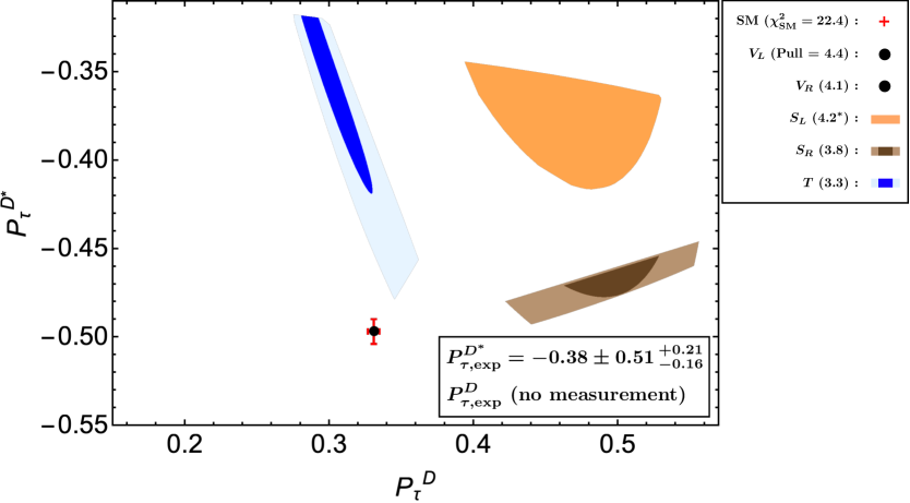
Figure 2: Predictions of $P_{\tau}^{D}$ and $P_{\tau}^{D^{\ast}}$ in the single complex NP operator scenarios. The allowed regions satisfying $\Delta\chi^{2}\leq 1$ ($4$) are shown in dark (light), orange, brown, and blue for the $C_{S_{L}}$, $C_{S_{R}}$, and $C_{T}$ scenarios, respectively, whereas the black dot is the case for the $C_{V_{L,R}}$ scenarios. The $B_{c}$ lifetime and LHC bounds are also taken into account. As for the $S_{L}$ scenario, the $B_{c}$ lifetime rules out the region for $\Delta\chi^{2}\leq 1$, whereas the LHC bound is not taken as discussed in the main text.

3.2 LQ scenarios

Finally, we study several LQ scenarios. It is well known that three categories of LQs can address the $R_{D^{(*)}}$ anomalies [74], which are referred to as a $SU(2)_{L}$-singlet vector $\text{U}_{1}^{\mu}$, a $SU(2)_{L}$-singlet scalar $\text{S}_{1}$, and a $SU(2)_{L}$-doublet scalar $\text{R}_{2}$. The relevant LQ interactions are given in Appendix A.

A key feature with respect to the fit is that these LQ scenarios involve three independent couplings relevant for $b\to c\tau\nu$, which are encoded in terms of the two independent (and complex in general) WCs as

$$\text{U}_{1}^{\mu}:~{} C_{V_{L}}\,,~{}C_{S_{R}}\,,$$ (3.7)

$$\text{S}_{1}:~{} C_{V_{L}}\,,~{}C_{S_{L}}=-4C_{T}\,,$$ (3.8)

$$\text{R}_{2}:~{} C_{V_{R}}\,,~{}C_{S_{L}}=4C_{T}\,,$$ (3.9)

at the LQ scale $\Lambda_{\text{LQ}}=M_{\text{LQ}}$. The $SU(2)_{L}$ doublet vector leptoquark $\text{V}_{2}$ forms $C_{S_{R}}$ [74], equivalent to the single $C_{S_{R}}$ scenario, and hence this LQ has now the viable solution as seen in Sec. 3.1. Flavor and collider phenomenologies of $\text{V}_{2}$ LQ could be interesting, but we leave it for a future work [108].

The $C_{V_{L}}$ phase in $|1+C_{V_{L}}|^{2}$ can be absorbed [42] in the flavor process. Thus, the absorption of the $C_{V_{L}}$ phase is irrelevant for the fit within the flavor observables and we take $C_{V_{L}}$ in $\text{U}_{1}$ and $\text{S}_{1}$ LQs as real without loss of generality. As for $C_{V_{R}}$ in the $\text{R}_{2}$ LQ, we assume it as pure imaginary from the fact of Eq. (3.3). Therefore, the three LQ scenarios of our interest have three degrees of freedom for the fit and the relevant observables, and then it is expected that fit results could be different from the previous studies.

These years, UV completions of the LQ scenarios have been studied in the literature; Refs. [109, 110, 111, 112, 113, 114, 115, 116, 117, 118, 119, 120, 121, 122, 123, 124] for $\text{U}_{1}$, Refs. [125, 126, 127] for $\text{S}_{1}$, Refs. [128, 129] for $\text{R}_{2}$, and see also Refs. [130, 131]. In the next subsection, we consider the case if the $\text{U}_{1}$ LQ is induced by a UV completed theory that gives a specific relation to the LQ couplings, and see how it changes the fit result. Recent re-evaluations on mass differences of the neutral $B$ mesons $\Delta M_{d},\,\Delta M_{s}$, (improved by HQET sum rule and lattice calculations [132]), would constrain a UV-completed TeV-scale LQ model [133, 126, 112, 111, 134, 124]. In particular, the ratio $\Delta M_{d}/\Delta M_{s}$ provides a striking constraint on the coupling texture of the LQ interactions. Here, we comment that a typical UV completion requires a vector-like lepton (VLL) and it induces LQ–VLL box diagrams that contribute to $\Delta M_{d,s}$. This implies that the constraint of our concern depends on the vector-like fermion mass spectrum, and hence we do not consider $\Delta M_{d,s}$ further in our analysis.

The LQ mass has been directly constrained as $M_{\text{LQ}}\gtrsim 1.5\,\text{TeV}$ from the LQ pair production searches [135, 136, 137]. Hence we take $M_{\text{LQ}}=2\,\text{TeV}$ for our benchmark scale. We recap that the WCs are bounded from the $\tau+\text{missing}$ search and, as shown in Table 3, the LQ scenarios receive milder constraints than the EFT operators as long as $M_{\text{LQ}}\leq 10\,\text{TeV}$.

The WCs will be fitted at the $\mu_{b}$ scale in our analysis, and then they are related to the WCs defined at the $\Lambda_{\text{LQ}}=M_{\text{LQ}}$ scale. The renormalization-group equations (RGEs) (the first matrix below) [138, 139, 140] and the LQ-charge independent QCD one-loop matching (the second one) [141] give the following relation

$$\begin{pmatrix}C_{V_{L}}(\mu_{b})\\ C_{V_{R}}(\mu_{b})\\ C_{S_{L}}(\mu_{b})\\ C_{S_{R}}(\mu_{b})\\ C_{T}(\mu_{b})\end{pmatrix} \simeq\begin{pmatrix}1&0&0&0&0\\ 0&1&0&0&0\\ 0&0&1.82&0&-0.35\\ 0&0&0&1.82&0\\ 0&0&-0.004&0&0.83\end{pmatrix}\begin{pmatrix}1.12&0&0&0&0\\ 0&1.07&0&0&0\\ 0&0&1.10&0&0\\ 0&0&0&1.05&0\\ 0&0&0&0&1.07\end{pmatrix}\begin{pmatrix}C_{V_{L}}(\Lambda_{\text{LQ}})\\ C_{V_{R}}(\Lambda_{\text{LQ}})\\ C_{S_{L}}(\Lambda_{\text{LQ}})\\ C_{S_{R}}(\Lambda_{\text{LQ}})\\ C_{T}(\Lambda_{\text{LQ}})\end{pmatrix}$$

$$\simeq\begin{pmatrix}1.12&0&0&0&0\\ 0&1.07&0&0&0\\ 0&0&1.91&0&-0.38\\ 0&0&0&2.00&0\\ 0&0&0.&0&0.89\end{pmatrix}\begin{pmatrix}C_{V_{L}}(\Lambda_{\text{LQ}})\\ C_{V_{R}}(\Lambda_{\text{LQ}})\\ C_{S_{L}}(\Lambda_{\text{LQ}})\\ C_{S_{R}}(\Lambda_{\text{LQ}})\\ C_{T}(\Lambda_{\text{LQ}})\end{pmatrix}\,,$$ (3.10)

with $\Lambda_{\text{LQ}}=2\,\text{TeV}$. Using these numbers, we obtain $C_{S_{L}}(\mu_{b})=-8.9\,C_{T}(\mu_{b})$ and $C_{S_{L}}(\mu_{b})=8.4\,C_{T}(\mu_{b})$ for $\text{S}_{1}$ and $\text{R}_{2}$ LQs, respectively.

With these ingredients, the LQ scenarios in terms of $C_{X}(\mu_{b})$ up to three degrees of freedom are investigated, where the full variable case is referred to as the general LQ. The results of the best fit points for the general LQ scenarios are then summarized as

$$\text{U}_{1}\text{~{}LQ}:~{} C_{V_{L}}=0.07\,,~{}C_{S_{R}}=0.06\,, \text{Pull}=3.8\,,$$ (3.11)

$$\text{S}_{1}\text{~{}LQ}:~{} C_{V_{L}}=0.06\,,~{}C_{S_{L}}=-8.9\,C_{T}=0.06\,, \text{Pull}=3.8\,,$$ (3.12)

$$\text{R}_{2}\text{~{}LQ}:~{} C_{V_{R}}=\pm i0.68\,,~{}C_{S_{L}}=8.4\,C_{T}=0.04\mp i0.65\,, \text{Pull}=3.8\,.$$ (3.13)

We observe that these three general LQ scenarios have the same Pull which means equivalently favored by the current data. We also see that $C_{S_{R}}$ ($C_{S_{L}}$) is preferred to be real at the best fit point for the $\text{U}_{1}$ ($\text{S}_{1}$) LQ scenario, whereas $C_{S_{L}}$ for $\text{R}_{2}$ LQ is given complex. The fit results for $\text{S}_{1}$ LQ and $\text{R}_{2}$ LQ with $C_{V_{L}}=C_{V_{R}}=0$ are obtained as

$$\text{S}_{1}\text{~{}LQ ($C_{V_{L}}=0$)}:~{} C_{S_{L}}=-8.9\,C_{T}=0.19\,, \text{Pull}=3.9\,,$$ (3.14)

$$\text{R}_{2}\text{~{}LQ ($C_{V_{R}}=0$)}:~{} C_{S_{L}}=8.4\,C_{T}=-0.07\pm i0.58\,, \text{Pull}=4.0\,,$$ (3.15)

where the improvements of Pull only come from the benefit of reducing the variables.

In turn, we evaluate the LHC bound on the two independent variables, such as $(C_{V_{L}},C_{S_{R}})$, by the following interpretation

$$\text{U}_{1}\text{~{}LQ}:~{}~{}\frac{|C_{V_{L}}(\mu_{b})|^{2}}{(0.42)^{2}}+\frac{|C_{S_{R}}(\mu_{b})|^{2}}{(0.77)^{2}}<1\,,$$ (3.16)

$$\text{S}_{1}\text{~{}LQ}:~{}~{}\frac{|C_{V_{L}}(\mu_{b})|^{2}}{(0.42)^{2}}+\frac{|C_{S_{L}}(\mu_{b})|^{2}}{(0.80)^{2}}<1\,,$$ (3.17)

$$\text{R}_{2}\text{~{}LQ}:~{}~{}\frac{|C_{V_{R}}(\mu_{b})|^{2}}{(0.51)^{2}}+\frac{|C_{S_{L}}(\mu_{b})|^{2}}{(0.80)^{2}}<1\,,$$ (3.18)

where the denominators are the current LHC bounds for the single WC scenarios with $M_{\text{LQ}}=2\,\text{TeV}$ from Table 3. Indeed this is a good approximation since the bound comes from the high-$p_{T}$ region that suppresses the interference term between the $V_{L,R}$ and $S_{L,R}$ operators. It can be seen that the best fit point of Eq. (3.13) for $\text{R}_{2}$ LQ is not consistent with the LHC bound of Eq. (3.18).

  Pull [$\chi^{2}_{\text{best}}$] Fitted $C_{X}$ Allowed region of $C_{X}$ Predictions $(\Delta\chi^{2}\leq 1)$ $B_{c}\to\tau\overline{\nu}$ LHC $P_{\tau}^{D}$ $-P_{\tau}^{D^{*}}$ $R_{J\mbox{\footnotesize$\!/\psi$}}$ SM –${~{}[22.4]}$ – – – $0.331\pm 0.004$ $0.497\pm 0.007$ $0.258\pm 0.004$ $\text{U}_{1}$ LQ $3.8~{}[2.2]$ $~{}~{}~{}\,C_{V_{L}}:\,[+0.04,+0.10]$ Eq. (2.9) Eq. (3.16) $[0.315,0.448]$ $[0.474,0.526]$ $[0.282,0.309]$ $\text{Re}C_{S_{R}}:\,[-0.02,+0.14]$ $\text{Im}C_{S_{R}}:\,[-0.46,+0.46]$ $\text{S}_{1}$ LQ $3.8~{}[2.4]$ $~{}~{}~{}\,C_{V_{L}}:\,[+0.02,+0.16]$ Eq. (2.9) Eq. (3.17) $[0.104,0.483]$ $[0.373,0.504]$ $[0.269,0.311]$ $\text{Re}C_{S_{L}}:\,[-0.05,+0.16]$ $\text{Im}C_{S_{L}}:\,[-0.50,+0.50]$ $\text{R}_{2}$ LQ $3.8~{}[2.0]$ $\text{Im}C_{V_{R}}:\,[\pm 0.00,\pm 0.50]$ Eq. (2.9) Eq. (3.18) $[0.286,0.492]$ $[0.404,0.537]$ $[0.280,0.311]$ $\text{Re}C_{S_{L}}:\,[-0.01,+0.08]$ $\text{Im}C_{S_{L}}:\,[\mp 0.00,\mp 0.39]$ $\text{R}_{2}$ LQ $4.0~{}[2.8]$ $\text{Re}C_{S_{L}}:\,[-0.13,-0.02]$ Eq. (2.9) Eq. (3.18) $[0.426,0.500]$ $[0.407,0.443]$ $[0.276,0.297]$ $(C_{V_{R}}=0)$ $\text{Im}C_{S_{L}}:\,[\pm 0.52,\pm 0.65]$  

Table 5: The fit results of the $\text{U}_{1}$, $\text{S}_{1}$, and $\text{R}_{2}$ LQ scenarios for $M_{\text{LQ}}=2\,\text{TeV}$. The WCs are given at the $\mu_{b}$ scale. The structure is the same as in Table 4.

In Table 5, we show our fit results and predictions with respect to the LQ scenarios like we did for the EFT cases. It is observed that the general LQ scenarios have less predictive values of the tau polarizations. This can be understood from the fact that the complex scalar WCs give large impacts on the interference terms as can be checked from Eqs. (2) and (2), which result in the wide ranges of the predictions.

Figure 3 visualizes the combined $P_{\tau}^{D}$–$P_{\tau}^{D^{*}}$ predictions satisfying $\Delta\chi^{2}\leq 1\,(4)$ and the aforementioned bounds, where the general $\text{U}_{1}$, $\text{S}_{1}$, and $\text{R}_{2}$ LQ scenarios are shown in dark (light) green, magenta, and yellow, respectively. The $\text{U}_{1}$ and $\text{R}_{2}$ LQ scenarios produce the correlated regions of the $P_{\tau}^{D}$–$P_{\tau}^{D^{*}}$ predictions and hence could be distinguished. On the other hand, the $\text{S}_{1}$ LQ scenario has the less-predictive wide region, which is hard to be identified.

Figure 3 also exhibits the predictions for the several specific scenarios, i.e., $\text{U}_{1}$ LQ with real WC (solid line), $\text{S}_{1}$ LQ with real WC (dashed line), and $\text{R}_{2}$ LQ with $C_{V_{R}}=0$ (gray region). It is seen that reducing the variable in the general LQ scenario provides the distinct prediction in particular for $P_{\tau}^{D^{*}}$ and the correlation for $P_{\tau}^{D}$–$P_{\tau}^{D^{*}}$ becomes a useful tool to identify the LQ signature. Therefore, it is significant to restrict the LQ interactions by other processes or by a UV theory that realizes the LQ particle. The latter will be discussed in the next subsection for the $\text{U}_{1}$ LQ (corresponding to the cyan region in the figure). Regarding the $\text{S}_{1}$ LQ scenario, we comment that a part of the allowed parameter region is ruled out by the $B\to K^{\ast}\nu\overline{\nu}$ measurement and $\Delta M_{s}$ (via LQ–$\nu_{\tau}$ box) [68].

Figure 3: Predictions of $P_{\tau}^{D}$ and $P_{\tau}^{D^{\ast}}$ in the LQ scenarios following the same procedure as in Fig. 2. The allowed regions are shown in dark (light) green, magenta, and yellow for the general $\text{U}_{1}$, $\text{S}_{1}$, and $\text{R}_{2}$ LQ scenarios, respectively. The specific scenarios; $\text{U}_{1}$ LQ with UV origin (cyan), real WC (solid line); $\text{S}_{1}$ LQ with real WC (dashed line); and $\text{R}_{2}$ LQ with $C_{V_{R}}=0$ (gray), are also given.

3.3 UV completion of $\text{U}_{1}$ LQ

As the $\text{U}_{1}$ LQ provides a unique solution, not only to the $b\to c\tau\nu$ anomaly, but also to several flavor issues, UV completions of the $U_{1}$ LQ have been discussed  [142, 143, 144, 145, 146, 147, 148, 149, 150]. A typical description is that the $\text{U}_{1}$ LQ is given as a gauge boson, embedded in a large gauge symmetry, such that the third-generation quarks and leptons are coupled to $U_{1}$ in the interaction basis. This means that the two LQ interactions of Eq. (A.1) are represented as a universal gauge coupling, $x_{L}^{33}=x_{R}^{33}\equiv g_{U}$ (see Appendix A). Moving to the mass basis leads to

$$C_{S_{R}}(\Lambda_{\text{LQ}})=-2\beta_{R}\times C_{V_{L}}(\Lambda_{\text{LQ}})\,,$$ (3.19)

where $\beta_{R}=e^{i\phi}$ denotes the relative complex (CP-violating) phase [149], which comes from the fact that the phases in the rotation matrices (to the mass basis) for quark and lepton are not necessarily identical. The LHC bound for this scenario has been studied and the typical scale of the constraint is obtained as $\Lambda_{\text{LQ}}\gtrsim 3.5\,\text{TeV}$ [111].

The RGE running effect changes the above relation of Eq. (3.19) at the $\mu_{b}$ scale of our interest. By taking $\Lambda_{\text{LQ}}=4\,\text{TeV}$ as a benchmark scale, we obtain

$$\begin{aligned} C_{V_{L}}(\mu_{b})&=1\times 1.11\times C_{V_{L}}(\Lambda_{\text{LQ}})\,,\\ C_{S_{R}}(\mu_{b})&=1.90\times 1.09\times C_{S_{R}}(\Lambda_{\text{LQ}})\,,\end{aligned}$$ (3.20)

where the first coefficient is the QCD two-loop RGE factor [140] and the second is the QCD one-loop matching correction [141] at the NP scale. Therefore, we have

$$C_{S_{R}}(\mu_{b})\simeq-3.7\,\beta_{R}\times C_{V_{L}}(\mu_{b})\,,$$ (3.21)

in the case of the UV origin $\text{U}_{1}$ LQ scenario, applied to our fit analysis.

The result of the best-fit point for the UV origin $\text{U}_{1}$ LQ scenario, with the definition of $\beta_{R}=e^{i\phi}$, is shown as

$$(C_{V_{L}},\phi)\,\simeq\,(0.07\,,\pm 0.54\pi) \text{Pull}=4.1\,.$$ (3.22)

One can see that this is consistent with the $B_{c}$ lifetime and LHC bounds. Predictions of the observables within $\Delta\chi^{2}\leq 1,4$ are then given in Fig. 3. It is observed that the large complex phase is favored which suppress the interference. It should be also stressed that the $\tau$ polarizations are so unique that this scenario can be distinguished from the aforementioned LQ scenarios.

4 The LFU violation in $\Upsilon$ decays

The UV completed NP models contributing to $b\to c\tau\overline{\nu}$ processes should also bring a related contribution to $b\overline{b}\to\tau^{+}\tau^{-}$ or $c\overline{c}\to\tau^{+}\tau^{-}$ interactions [28, 151, 152]. In this section, we show that $\text{U}_{1}$ and $\text{R}_{2}$ LQs predict a robust correlation between $b\to c\tau\overline{\nu}$ and $b\overline{b}\to\tau^{+}\tau^{-}$ via the LQ exchange.

A definition of the LFU observable in the $\Upsilon(nS)$ decays is

$$R_{\Upsilon(nS)}\equiv\frac{\mathcal{B}(\Upsilon(nS)\to\tau^{+}\tau^{-})}{\mathcal{B}(\Upsilon(nS)\to\ell^{+}\ell^{-})}\,,$$ (4.1)

with $n=1,2,3$, where $R_{\Upsilon(nS)}\simeq 1$ holds in the SM. As for $n\geq 4$, the leptonic branching ratios are significantly suppressed since a $B\kern 1.79993pt\overline{\kern-1.79993ptB}{}$ decay channel is open. Since the short- and long-distance QCD corrections [154] are independent of the lepton mass, they are canceled in this ratio. One can also discuss the $c\overline{c}\to l^{+}l^{-}$ LFU observable via $\psi(2S)$ decays. However, we do not consider it because the present experimental error is relatively large.

Recently, the BaBar collaboration has reported a precise result for measurement of $R_{\Upsilon(3S)}$ [73]: $R_{\Upsilon(3S)}^{\rm BaBar}=0.966\pm 0.008_{\rm stat}\pm 0.014_{\rm syst},$ where $\ell=\mu$. Combing a previous measurement by the CLEO collaboration [155], an average for the $\Upsilon(3S)$ decay is [151]

$$R_{\Upsilon(3S)}^{\rm exp}=0.968\pm 0.016\,.$$ (4.2)

This value is consistent with the SM prediction [28]

$$R_{\Upsilon(3S)}^{\rm SM}=0.9948\pm\mathcal{O}(10^{-5})\,,$$ (4.3)

at the $1.7\sigma$ level. The SM prediction slightly deviates from $1$ whose leading correction comes from the difference in the phase space factor between the $\tau/\ell$ modes [156]. The next-to-leading contribution comes from the QED correction which depends on the lepton mass [157]; $\delta_{\rm EM}R_{\Upsilon(nS)}=+0.0002$. The tree-level $Z$ exchange also contributes, but its effect is $\mathcal{O}(10^{-5})$ [28]. There is no Higgs boson contribution as one can see below. The other channels ($n=1,2$) still suffer from the current experimental uncertainty, and we do not utilize them in our presentation.

The effective Hamiltonian which is relevant to the bottomonium decay into $\tau^{+}\tau^{-}$ is described as

$$-\mathcal{H}^{\rm NP}_{\rm eff}= ~{}C_{VLL}^{b\tau}(\overline{b}\gamma^{\mu}P_{L}b)(\overline{\tau}\gamma_{\mu}P_{L}\tau)+C_{VRR}^{b\tau}(\overline{b}\gamma^{\mu}P_{R}b)(\overline{\tau}\gamma_{\mu}P_{R}\tau)$$

$$+C_{VLR}^{b\tau}(\overline{b}\gamma^{\mu}P_{L}b)(\overline{\tau}\gamma_{\mu}P_{R}\tau)+C_{VRL}^{b\tau}(\overline{b}\gamma^{\mu}P_{R}b)(\overline{\tau}\gamma_{\mu}P_{L}\tau)$$ (4.4)

$$+\left[C_{T}^{b\tau}(\overline{b}\sigma^{\mu\nu}P_{R}b)(\overline{\tau}\sigma_{\mu\nu}P_{R}\tau)+C_{SL}^{b\tau}(\overline{b}P_{L}b)(\overline{\tau}P_{L}\tau)+C_{SR}^{b\tau}(\overline{b}P_{R}b)(\overline{\tau}P_{L}\tau)+\textrm{h.c.}\right]\,,$$

at the scale $\mu=m_{\Upsilon}$. Note that $C_{VLL}^{b\tau},C_{VRR}^{b\tau},C_{VLR}^{b\tau}$ and $C_{VRL}^{b\tau}$ are real coefficients, and $C_{SL}^{b\tau}$ and $C_{SR}^{b\tau}$ never contribute to the $\Upsilon(nS)\to\tau^{+}\tau^{-}$ due to $\langle 0|\overline{b}b|\Upsilon\rangle=\langle 0|\overline{b}\gamma_{5}b|\Upsilon\rangle=0$. In this convention, the partial decay width is given by [28]

$$\begin{aligned} \Gamma(\Upsilon(nS)\to\tau^{+}\tau^{-})=&~{}\frac{f_{\Upsilon}^{2}}{4\pi m_{\Upsilon}}\sqrt{1-4x_{\tau}^{2}}\Bigl{[}A_{\Upsilon}^{2}(1+2x_{\tau}^{2})+B_{\Upsilon}^{2}(1-4x_{\tau}^{2})\\ &\quad+\frac{1}{2}C_{\Upsilon}^{2}(1-4x_{\tau}^{2})^{2}+\frac{1}{2}D_{\Upsilon}^{2}(1-4x_{\tau}^{2})+2A_{\Upsilon}C_{\Upsilon}x_{\tau}(1-4x_{\tau}^{2})\Bigr{]}\,,\end{aligned}$$ (4.5)

with

$$A_{\Upsilon}= \frac{4\pi\alpha}{3}+\frac{m_{\Upsilon}^{2}}{4}\left[C_{VLL}^{b\tau}+C_{VRR}^{b\tau}+C_{VLR}^{b\tau}+C_{VRL}^{b\tau}+16x_{\tau}\frac{f_{\Upsilon}^{T}}{f_{\Upsilon}}\textrm{Re}\left(C_{T}^{b\tau}\right)\right]\,,$$ (4.6)

$$B_{\Upsilon}= \frac{m_{\Upsilon}^{2}}{4}\left(C_{VRR}^{b\tau}+C_{VLR}^{b\tau}-C_{VLL}^{b\tau}-C_{VRL}^{b\tau}\right)\,,$$ (4.7)

$$C_{\Upsilon}= 2m_{\Upsilon}^{2}\frac{f_{\Upsilon}^{T}}{f_{\Upsilon}}\textrm{Re}\left(C_{T}^{b\tau}\right)\,,$$ (4.8)

$$D_{\Upsilon}= 2m_{\Upsilon}^{2}\frac{f_{\Upsilon}^{T}}{f_{\Upsilon}}\textrm{Im}\left(C_{T}^{b\tau}\right)\,,$$ (4.9)

and

$$x_{\tau}=\frac{m_{\tau}}{m_{\Upsilon}}\,.$$ (4.10)

The $f_{\Upsilon}$ and $f_{\Upsilon}^{T}$ are form factors for vector and tensor currents in $\Upsilon$ hadronic-matrix elements, and $f_{\Upsilon}=f_{\Upsilon}^{T}$ holds in the heavy quark limit, which is realized for the $\Upsilon$ decays [28].

Within the SM, this process is predominantly caused by the QED. Nevertheless, the photon-exchange QED contribution is suppressed by $1/m_{\Upsilon}^{2}$, and hence the NP contribution could be non-negligible [28, 158, 151]. In the SM, $A_{\Upsilon}\simeq 4\pi\alpha/3$ and $B_{\Upsilon},C_{\Upsilon},D_{\Upsilon}\simeq 0$. Setting the light lepton mass to zero and $m_{\Upsilon}=m_{\Upsilon(3S)}=10.355\,\text{GeV}$, we obtain the following numerical formula

$$\begin{aligned} \frac{R_{\Upsilon(3S)}}{R_{\Upsilon(3S)}^{\rm SM}}=&~{}1+1.64\times 10^{-3}\ {\rm TeV}^{2}\left(C_{VLL}^{b\tau}+C_{VRR}^{b\tau}+C_{VLR}^{b\tau}+C_{VRL}^{b\tau}\right)\\ &+6.37\times 10^{-3}\ {\rm TeV}^{2}\ \textrm{Re}\left(C_{T}^{b\tau}\right)+\delta_{\Upsilon}\,,\end{aligned}$$ (4.11)

with

$$\begin{aligned} \delta_{\Upsilon}=&~{}5.22\times 10^{-6}\ {\rm TeV}^{4}\left(C_{VLL}^{b\tau}+C_{VRR}^{b\tau}+C_{VLR}^{b\tau}+C_{VRL}^{b\tau}\right)\textrm{Re}\left(C_{T}^{b\tau}\right)\\ &+6.71\times 10^{-7}\ {\rm TeV}^{4}\left(C_{VLL}^{b\tau}+C_{VRR}^{b\tau}+C_{VLR}^{b\tau}+C_{VRL}^{b\tau}\right)^{2}\\ &+5.59\times 10^{-7}\ {\rm TeV}^{4}\left(C_{VRR}^{b\tau}+C_{VLR}^{b\tau}-C_{VLL}^{b\tau}-C_{VRL}^{b\tau}\right)^{2}\\ &+2.51\times 10^{-5}\ {\rm TeV}^{4}\left[\textrm{Re}\left(C_{T}^{b\tau}\right)\right]^{2}+1.79\times 10^{-5}\ {\rm TeV}^{4}\left[\textrm{Im}\left(C_{T}^{b\tau}\right)\right]^{2}\,,\end{aligned}$$ (4.12)

where the $\delta_{\Upsilon}$ term gives negligible contributions.

Let us now look into a correlation between $R_{\Upsilon(3S)}$ and $R_{D^{(\ast)}}$ by using the specific examples of the $\text{U}_{1}$ and $\text{R}_{2}$ LQs. First, we exhibit the $\text{U}_{1}$ LQ case. The $\text{U}_{1}$ LQ interaction with the SM fermions is given in Eq. (A.1). Integrating the $\text{U}_{1}$ LQ out, as well as the charged current contributions ($b\to c\tau\overline{\nu}$) in Eq. (A.2), the neutral current ones ($b\overline{b}\to\tau^{+}\tau^{-}$) are obtained as

$$C_{VLL}^{b\tau}(\mu_{\rm LQ})=-\frac{|x_{L}^{b\tau}|^{2}}{m_{U_{1}}^{2}}\,,\quad C_{VRR}^{b\tau}(\mu_{\rm LQ})=-\frac{|x_{R}^{b\tau}|^{2}}{m_{U_{1}}^{2}}\,,\quad C_{SR}^{b\tau}(\mu_{\rm LQ})=\frac{2x_{L}^{b\tau}(x_{R}^{b\tau})^{\ast}}{m_{U_{1}}^{2}}\,.$$ (4.13)

The vector contributions do not change under the RGEs, while the scalar contribution does not affect the $\Upsilon$ decay. Here, an important point is that $R_{\Upsilon(3S)}/R_{\Upsilon(3S)}^{\rm SM}$ is predicted to be less than $1$ when NP contributions are dominated by vector interactions. It would lead to a coherent deviation with $R_{D^{(\ast)}}$.

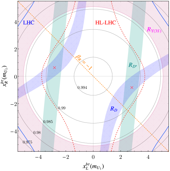
Figure 4: The correlation between $R_{\Upsilon(3S)}$ and $R_{D^{(\ast)}}$ is exhibited in the $\text{U}_{1}$ LQ scenario with $m_{\text{U}_{1}}=2\,$TeV by setting $(Vx_{L})^{c\tau}=V_{cb}x_{L}^{b\tau}$. The predicted values of $R_{\Upsilon(3S)}$ are shown by black contours, and $R_{\Upsilon(3S)}^{\rm exp}$ in Eq. (4.2) is shown in the red shaded area. $R_{D}$ and $R_{D^{\ast}}$ anomalies can be explained in the blue and green regions, respectively. The LHC exclusion region (outside the blue line) and the HL-LHC sensitivity (red dashed line) are based on the result of Table 3. The best fit points of Eq. (3.11) are shown by red crosses. The orange dashed line represents the $U(2)$ flavor symmetry prediction with $\beta_{R}=-1$.

Setting $m_{U_{1}}=2.0\,\text{TeV}$ and $(Vx_{L}(\mu_{\text{LQ}}))^{c\tau}=V_{cb}x_{L}^{b\tau}(\mu_{\text{LQ}})$, namely $x_{L}^{s\tau}(\mu_{\text{LQ}})=0$, we show a correlation between $R_{\Upsilon(3S)}$ and $R_{D^{(\ast)}}$ in Fig. 4. Here, favored parameter regions in the $\text{U}_{1}$ LQ model are exhibited on $x_{L}^{b\tau}$–$x_{R}^{b\tau}$ plane at the renormalization scale $\mu_{\text{LQ}}=m_{U_{1}}$. The black contour represents the expected values of $R_{\Upsilon(3S)}$. The red shaded region is favored by $R_{\Upsilon(3S)}^{\rm exp}$ in Eq. (4.2). It is noted that if we adopt the $2\sigma$ constraint of $R_{\Upsilon(3S)}^{\rm exp}$, the entire parameter region is allowed. The blue and green regions can explain the $R_{D}$ and $R_{D^{\ast}}$ discrepancies within $1\sigma$, respectively. The exclusion region by the LHC analysis ($\tau+\,$missing search) is outside the blue line, while the future prospect of the High Luminosity LHC (HL-LHC) is shown by the red dashed line, see Table 3. Furthermore, the orange dashed line stands for a prediction in the case of the UV origin $\text{U}_{1}$ LQ with $\beta_{R}=-1~{}(\phi=\pi)$. From the figure, it is found that the current $R_{\Upsilon(3S)}^{\rm exp}$ overshoots favored parameter region from the $R_{D^{(*)}}$ anomalies. The best fit points of Eq. (3.11) are shown by red crosses and predict $R_{\Upsilon(3S)}=0.991$, distinct from the 0.99 contour line in the figure. Thus, it seems crucial to measure $R_{\Upsilon(nS)}$ with less than $1\%$ accuracy in order to distinguish the $\text{U}_{1}$ LQ signal.

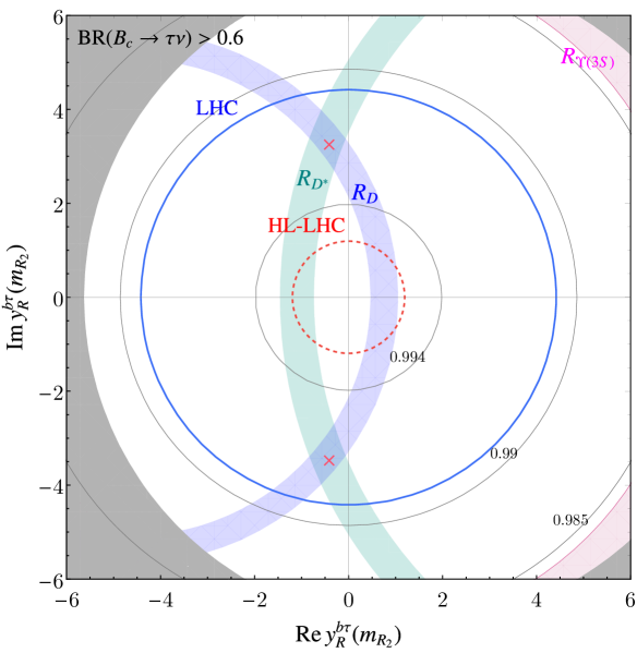
Figure 5: Correlation between $R_{\Upsilon(3S)}$ and $R_{D^{(\ast)}}$ in the $\text{R}_{2}$ LQ scenario with $m_{\text{R}_{2}}=2\,$TeV and $y_{L}^{c\tau}=1$. The color convention is the same as in Fig. 4. The gray shaded region is excluded by the $B_{c}$ lifetime. The best fit points of Eq. (3.15) are shown by red crosses.

Next, we investigate the $\text{R}_{2}$ LQ scenario. The $\text{R}_{2}$ LQ interaction with the SM fermions is given in Eq. (A.6). The generated charged current contributions are given in Eq. (A.7), while the neutral current one is

$$C_{VLR}^{b\tau}(\mu_{\rm LQ})=-\frac{|y_{R}^{b\tau}|^{2}}{2m_{R_{2}}^{2}}\,.$$ (4.14)

Since $C_{VLR}^{b\tau}<0$, $R_{\Upsilon(3S)}/R_{\Upsilon(3S)}^{\rm SM}$ has to be less than $1$ again.

The result is shown in Fig. 5. Here, we set $y_{L}^{c\tau}(\mu_{\rm LQ})=1$, $|V_{cb}|=0.04$, and $m_{\text{R}_{2}}=2.0\,$TeV, and take $y_{R}^{b\tau}(\mu_{\rm LQ})$ as complex value. The color convention is the same as the $\text{U}_{1}$ LQ case. Furthermore, the gray shaded region is excluded by the $B_{c}$ lifetime, i.e., $\mathcal{B}(B_{c}\to\tau\overline{\nu})>0.6$. The best fit points in Eq. (3.15) are shown by red crosses, predicting $R_{\Upsilon(3S)}=0.992$. Similar to $\text{U}_{1}$ LQ interpretation, $1\%$ accuracy of the $R_{\Upsilon(nS)}$ measurement is required as the $\text{R}_{2}$ LQ signature.

At the current stage, the large experimental uncertainty in $R_{\Upsilon(3S)}$ cannot allow a clear-cut conclusion. One should note that the Belle and Belle II experiments have enough sensitivities to the $R_{\Upsilon(nS)}$ measurements which would be more accurate than the existing BaBar measurement [159].

5 Conclusions and discussion

	Spin	Charge	Operators	$R_{D}$	$R_{D^{*}}$	LHC	Flavor
$H^{\pm}$	0	($\bf{1}$, $\bf{2}$, $\nicefrac{{1}}{{2}}$)	$O_{S_{L}}$	${\Large{\color[rgb]{0,.5,.5}{\bf{\checkmark}}}}$	${\Large{\color[rgb]{0,.5,.5}{\bf{\checkmark}}}}$	$b\tau\nu$	$B_{c}\to\tau\nu$, $F_{L}^{D^{\ast}}$, $P^{D}_{\tau}$, $M_{W}$
$\text{S}_{1}$	0	($\bf{\bar{3}}$, $\bf{1}$, $\nicefrac{{1}}{{3}}$)	$O_{V_{L}}$, $O_{S_{L}}$, $O_{T}$	${\Large{\color[rgb]{0,.5,.5}{\bf{\checkmark}}}}$	${\Large{\color[rgb]{0,.5,.5}{\bf{\checkmark}}}}$	$\tau\tau$	$\Delta M_{s}$, $P_{\tau}^{D}$, $B\to K^{(\ast)}\nu\nu$
$\text{R}_{2}^{(\nicefrac{{2}}{{3}})}$	0	($\bf{3}$, $\bf{2}$, $\nicefrac{{7}}{{6}}$)	$O_{S_{L}}$, $O_{T}$, ($O_{V_{R}}$)	${\Large{\color[rgb]{0,.5,.5}{\bf{\checkmark}}}}$	${\Large{\color[rgb]{0,.5,.5}{\bf{\checkmark}}}}$	$b\tau\nu$, $\tau\tau$	$R_{\Upsilon(nS)}$, $P_{\tau}^{D^{\ast}}$, $M_{W}$
$\text{U}_{1}$	1	($\bf{3}$, $\bf{1}$, $\nicefrac{{2}}{{3}}$)	$O_{V_{L}}$, $O_{S_{R}}$	${\Large{\color[rgb]{0,.5,.5}{\bf{\checkmark}}}}$	${\Large{\color[rgb]{0,.5,.5}{\bf{\checkmark}}}}$	$b\tau\nu$, $\tau\tau$	$R_{K^{(\ast)}}$, $R_{\Upsilon(nS)}$, $B_{s}\to\tau\tau$
$\text{V}_{2}^{(\nicefrac{{1}}{{3}})}$	1	($\bf{\bar{3}}$, $\bf{2}$, $\nicefrac{{5}}{{6}}$)	$O_{S_{R}}$	${\Large{\color[rgb]{0,.5,.5}{\bf{\checkmark}}}}$	${2\sigma}$	$\tau\tau$	$B_{s}\to\tau\tau$, $M_{W}$

Table 6: Summary table for the single-mediator NP scenarios in light of the $b\to c\tau\nu$ anomaly. We add implications for the LHC searches and flavor observables in the last two columns, which is useful to identify the NP scenario. In the $\text{V}_{2}^{(\nicefrac{{1}}{{3}})}$ LQ scenario, $2\sigma$ for $R_{D^{\ast}}$ implies that it can explain the $R_{D^{\ast}}$ anomaly within the $2\sigma$ range (but not within $1\sigma$).

In this work we revisited our previous phenomenological investigation and presented a statistical analysis of the LFU violation in $R_{D^{(*)}}$, including the new experimental data from the LHCb experiment. Starting with the re-evaluation of the generic formulae for $R_{D^{(*)}}$ by employing the recent development of the $B\to D^{(\ast)}$ transition form factors, we examined the new physics possibility with the low-energy effective Lagrangian as well as the leptoquark models. In addition to the constraints from the low-energy observables and the high-$p_{T}$ mono-$\tau$ search at LHC, the predictions on the relevant observables of $R_{\Upsilon}$, $R_{J\mbox{\footnotesize$\!/\psi$}}$, and the tau polarizations $P_{\tau}^{D^{(*)}}$ are evaluated.

To be precise, we performed the $\chi^{2}$ fit to the experimental measurements of $R_{D^{(*)}}$ and the $D^{*}$ polarization $F_{L}^{D^{*}}$. This updated analysis shows that the present data deviates from the SM predictions at $\sim 4\sigma$ level. Our fit result is summarized in Table 4 with Eqs. (3.3)–(3.5) for the single-operator scenarios, and Table 5 with Eqs. (3.11)–(3.15), (3.22) for the single-mediator leptoquark scenarios. The NP fit improvements compared with the SM one are visualized by Pull as usual, and it was found that the SM-like vector operator still gives the best Pull.

Due to the new LHCb result, the experimental world average has slightly come close to the SM predictions of $R_{D}$ and $R_{D^{*}}$. This change has affected the previous conclusions such that the scalar NP solutions to the $b\to c\tau\nu$ anomaly had been disfavored. Namely, the scalar NP interpretations have been revived now. On the other hand, it is found that the results of the LQ scenarios do not drastically change, compared with the previous fit.

As it was pointed out in the literature, the precise measurements of the polarization observables $P_{\tau}^{D^{(*)}}$ and $F_{L}^{D^{*}}$ have the potential to distinguish the NP scenarios. In Figs. 2 and 3, we show our predictions of $P_{\tau}^{D}$ and $P_{\tau}^{D^{*}}$ for the possible NP scenarios. One can make sure that the single-operator NP scenario explaining the $b\to c\tau\nu$ anomaly can be identified by the $P_{\tau}^{D^{(*)}}$ measurements, which may be available at the Belle II experiment. On the other hand, the general LQ scenarios are hard to be distinguished due to predicting wide ranges of $P_{\tau}^{D^{(*)}}$. Once the LQ model with restricted interactions is constructed, however, we see that the $P_{\tau}^{D^{(*)}}$ measurement has significant potential to probe the LQ signature. The high energy collider search is also important since the high-$p_{T}$ lepton search at the LHC can directly probe the NP interactions affecting the LFU ratios.

We also investigated the NP impacts on the LFU violation in the $\Upsilon(nS)$ decays. We found that the LFU ratio $R_{\Upsilon}$ has to be correlated to $R_{D^{(\ast)}}$ in the $\text{U}_{1}$ and $\text{R}_{2}$ LQ scenarios, while no correlation is expected in the $\text{S}_{1}$ LQ scenario. It is shown that an experimental accuracy of less than $1\%$ for the $R_{\Upsilon(nS)}$ measurement is necessary in order to identify the LQ scenario. We expect that this is possible in the Belle II experiment.

In Table 6, we put a summary check sheet to find which single-mediator NP scenarios are viable and to see important observables in order to identify the NP scenario responsible for the $b\to c\tau\nu$ anomaly.

Furthermore, it is known that the baryonic counterpart of $R_{D^{(*)}}$, namely $R_{\Lambda_{c}}\equiv\mathcal{B}(\Lambda_{b}\to\Lambda_{c}\,\tau\overline{\nu})/\mathcal{B}(\Lambda_{b}\to\Lambda_{c}\,\mu\overline{\nu})$, provides the independent cross check of the $b\to c\tau\nu$ anomaly [43, 44]. Recently, $R_{\Lambda_{c}}$ has been measured for the first time as $R_{\Lambda_{c}}=0.242\pm 0.026\pm 0.040\pm 0.059$ by the LHCb experiment [160], where the last dominant uncertainty comes from an external branching fraction from the LEP measurement [161]. This result implies consistency with the SM prediction at $1.1\sigma$ level [27, 162], while, instead, normalizing with the SM prediction of $\Gamma(\Lambda_{b}\to\Lambda_{c}\mu\overline{\nu})$ improves the accuracy and slightly up-lifts the central value, e.g., $R_{\Lambda_{c}}=|0.04/V_{cb}|^{2}(0.285\pm 0.073)$ [163]. Even though the current experimental uncertainty is not enough precise, it could already provide a nontrivial constraint on the NP parameter space which can explain the $b\to c\tau\nu$ anomaly. An implication of the measured $R_{\Lambda_{c}}$ for NP models is given in Ref. [164].

Appendix A Leptoquark interactions

The LQ interactions are classified with the generic $SU(3)_{c}\times SU(2)_{L}\times U(1)_{Y}$ invariant form [165]. We leave details of the model constructions, and then just introduce the interactions relevant for $b\to c\tau\overline{\nu}$. As mentioned above, there are three viable candidates of leptoquark $\text{U}_{1},~{}\text{S}_{1},~{}\text{R}_{2}$[166]. Their quantum numbers under $SU(3)_{\rm{C}}$, $SU(2)_{\rm{L}}$, $U(1)_{\rm{Y}}$ are summarized in Table 6.

First, the $\text{U}_{1}$ vector LQ interaction with the SM fermions, defined in the interaction basis, is given by

$$\mathcal{L}_{U_{1}}=\hat{x}^{ij}_{L}\overline{Q}_{i}\gamma_{\mu}U^{\mu}_{1}L_{j}+\hat{x}^{ij}_{R}\overline{d}_{Ri}\gamma_{\mu}U^{\mu}_{1}\ell_{Rj}+\textrm{h.c.}\,.$$ (A.1)

Integrating out the $\text{U}_{1}$ LQ mediator particle, then, the Wilson coefficients (WCs) for the charged current of our interest ($b\to c\tau\overline{\nu}$) is obtained as

$$\begin{aligned} C_{V_{L}}(\mu_{\rm LQ})&=\frac{1}{2\sqrt{2}G_{F}V_{cb}}\frac{(Vx_{L})^{c\tau}(x_{L}^{b\tau})^{\ast}}{m_{U_{1}}^{2}}\,,\\ C_{S_{R}}(\mu_{\rm LQ})&=-\frac{1}{\sqrt{2}G_{F}V_{cb}}\frac{(Vx_{L})^{c\tau}(x_{R}^{b\tau})^{\ast}}{m_{U_{1}}^{2}}\,,\end{aligned}$$ (A.2)

where $V$ is the CKM matrix and the couplings $x_{L,R}$ are in the mass basis. The relative sign and factor two in Eq. (A.2) come from the property of Fierz identity.

In a typical UV completed theory [149], the $\text{U}_{1}$ LQ is realized as a gauge boson generated from a large gauge symmetry and only couples to the third-generation SM fermions. Namely, $\hat{x}_{R}^{b\tau}=\hat{x}_{L}^{b\tau}\equiv g_{U}$, with the others to be zero, is indicated in the gauge interaction basis. Moving to the mass basis, then, generates a non-zero off-diagonal part such as $x_{L}^{c\tau}$ and also $x_{R}^{b\tau}=e^{i\phi}x_{L}^{b\tau}$, where the phase comes from those in the rotation matrices to the mass bases of the left- and right-handed quark and lepton fields that are not canceled in general. Therefore, the UV completion of $\text{U}_{1}$ LQ suggests

$$C_{S_{R}}(\mu_{\rm LQ})=-2e^{i\phi}C_{V_{L}}(\mu_{\rm LQ})\,,$$ (A.3)

as introduced in the main text. We also comment that an extension of the fermion families with a nontrivial texture of the fermion mass matrices is necessary to construct a practical UV model [123].

The $\text{S}_{1}$ scalar LQ interaction in the mass basis is given by

$$\mathcal{L}_{{\rm S}_{1}} =\big{(}V^{\ast}y_{L}\big{)}^{ij}\,\overline{u^{C}_{L\,i}}\ell_{L\,j}{\rm S}_{1}-y_{L}^{ij}\,\overline{d^{C}_{L\,i}}\nu_{L\,j}{\rm S}_{1}+y_{R}^{ij}\,\overline{u^{C}_{R\,i}}\ell_{R\,j}{\rm S}_{1}+\mathrm{h.c.}\,.$$ (A.4)

In the scalar LQ scenario, the source of the generation violating couplings is off-diagonal element of Yukawa matrices. Then the four-fermion interactions of $b\to c\tau{\overline{\nu}}$ are given by

$$\begin{aligned} C_{S_{L}}(\mu_{\rm LQ})&=-4\,C_{T}(\mu_{\rm LQ})=-\dfrac{1}{4\sqrt{2}G_{F}V_{cb}}\dfrac{y_{L}^{b{\tau}}\big{(}y_{R}^{c\tau}\big{)}^{\ast}}{m_{S_{1}}^{2}}\,,\\ C_{V_{L}}(\mu_{\rm LQ})&=\dfrac{1}{4\sqrt{2}G_{F}V_{cb}}\dfrac{y_{L}^{b\tau}\big{(}Vy_{L}^{\ast}\big{)}^{c\tau}}{m_{S_{1}}^{2}}\,.\end{aligned}$$ (A.5)

Finally, we introduce the $\text{R}_{2}$ scalar LQ interaction. $\text{R}_{2}$ is a SU(2) doublet and a component with $2/3$ of the electromagnetic charge ${\rm R}_{2}^{(\nicefrac{{2}}{{3}})}$ can contribute to $b\to c\tau{\overline{\nu}}$. The Yukawa interaction

$$\mathcal{L}_{{\rm R}_{2}}=y_{R}^{ij}\,\overline{d}_{L\,i}\ell_{R\,j}\,{\rm R}_{2}^{(\nicefrac{{2}}{{3}})}+y_{L}^{ij}\overline{u}_{R\,i}\nu_{L\,j}\,{\rm R}_{2}^{(\nicefrac{{2}}{{3}})}+\mathrm{h.c.}\,,$$ (A.6)

gives

$$C_{S_{L}}(\mu_{\rm LQ}) =4\,C_{T}(\mu_{\rm LQ})=\dfrac{1}{4\sqrt{2}G_{F}V_{cb}}\dfrac{y_{L}^{c\tau}\big{(}y_{R}^{b\tau}\big{)}^{\ast}}{m_{R_{2}}^{2}}\,.$$ (A.7)

In contrast to the above two LQ scenarios, the $\text{R}_{2}$ LQ does not generate $C_{V_{L}}$ but $C_{V_{R}}$. Thus we could expect solid predictions in polarization and related observables. To generate $C_{V_{R}}$, indeed, a large mixing between two distinct $\text{R}_{2}$ LQ doublet is required to induce a proper electroweak symmetry breaking. See details in Refs. [85, 68].

References

- [1] BaBar Collaboration, “Evidence for an excess of decays,” Phys. Rev. Lett. 109 (2012) 101802 [arXiv:1205.5442].
- [2] BaBar Collaboration, “Measurement of an Excess of Decays and Implications for Charged Higgs Bosons,” Phys. Rev. D 88 (2013) 072012 [arXiv:1303.0571].
- [3] Belle Collaboration, “Measurement of the branching ratio of relative to decays with hadronic tagging at Belle,” Phys. Rev. D 92 (2015) 072014 [arXiv:1507.03233].
- [4] Belle Collaboration, “Measurement of the lepton polarization and in the decay ,” Phys. Rev. Lett. 118 (2017) 211801 [arXiv:1612.00529].
- [5] Belle Collaboration, “Measurement of the lepton polarization and in the decay with one-prong hadronic decays at Belle,” Phys. Rev. D 97 (2018) 012004 [arXiv:1709.00129].
- [6] Belle Collaboration, “Measurement of and with a semileptonic tagging method.” arXiv:1904.08794.
- [7] Belle Collaboration, “Measurement of and with a semileptonic tagging method,” Phys. Rev. Lett. 124 (2020) 161803 [arXiv:1910.05864].
- [8] LHCb Collaboration, “Measurement of the ratio of branching fractions ,” Phys. Rev. Lett. 115 (2015) 111803 [arXiv:1506.08614]. [Erratum: Phys.Rev.Lett. 115, 159901 (2015)].
- [9] LHCb Collaboration, “Measurement of the ratio of the and branching fractions using three-prong -lepton decays,” Phys. Rev. Lett. 120 (2018) 171802 [arXiv:1708.08856].
- [10] LHCb Collaboration, “Test of Lepton Flavor Universality by the measurement of the branching fraction using three-prong decays,” Phys. Rev. D 97 (2018) 072013 [arXiv:1711.02505].
- [11] D. London and J. Matias, “ Flavour Anomalies: 2021 Theoretical Status Report,” Ann. Rev. Nucl. Part. Sci. 72 (2022) 37–68 [arXiv:2110.13270].
- [12] Belle-II Collaboration, “First flavor tagging calibration using 2019 Belle II data.” arXiv:2008.02707.
- [13] Belle-II Collaboration, “Snowmass White Paper: Belle II physics reach and plans for the next decade and beyond.” arXiv:2207.06307.
- [14] G. Landsberg, “B Physics Parking Program in CMS.” talk in 20th Annual RDMS CMS Collaboration Conference, 2018.
- [15] CMS Collaboration, “Recording and reconstructing 10 billion unbiased b hadron decays in CMS,” 2019. https://cds.cern.ch/record/2704495.
- [16] R. Bainbridge, “Recording and reconstructing 10 billion unbiased b hadron decays in CMS,” EPJ Web Conf. 245 (2020) 01025.
- [17] Y. Takahashi, “Indications of new physics beyond the Standard Model in flavor anomalies observed at the LHC experiments.” talk in The Physical Society of Japan 2020 Autumn meeting, 2020.
- [18] LHCb Collaboration, “ and with .”. https://indico.cern.ch/event/1187939/.
- [19] HFLAV Collaboration. “Average of and for End of 2022” at https://hflav-eos.web.cern.ch/hflav-eos/semi/fall22/html/RDsDsstar/RDRDs.html.
- [20] HFLAV Collaboration, “Averages of -hadron, -hadron, and -lepton properties as of 2021.” arXiv:2206.07501. Average of and for Spring 2021 at https://hflav-eos.web.cern.ch/hflav-eos/semi/spring21/html/RDsDsstar/RDRDs.html.
- [21] F. U. Bernlochner, M. F. Sevilla, D. J. Robinson, and G. Wormser, “Semitauonic b-hadron decays: A lepton flavor universality laboratory,” Rev. Mod. Phys. 94 (2022) 015003 [arXiv:2101.08326].
- [22] F. U. Bernlochner, et al., “Constrained second-order power corrections in HQET: R(D(*)), —Vcb—, and new physics,” Phys. Rev. D 106 (2022) 096015 [arXiv:2206.11281].
- [23] S. Iguro and R. Watanabe, “Bayesian fit analysis to full distribution data of determination and new physics constraints,” JHEP 08 (2020) 006 [arXiv:2004.10208].
- [24] M. Bordone, M. Jung, and D. van Dyk, “Theory determination of form factors at ,” Eur. Phys. J. C 80 (2020) 74 [arXiv:1908.09398].
- [25] M. Bordone, N. Gubernari, D. van Dyk, and M. Jung, “Heavy-Quark expansion for form factors and unitarity bounds beyond the limit,” Eur. Phys. J. C 80 (2020) 347 [arXiv:1912.09335].
- [26] LATTICE-HPQCD Collaboration, “ and Lepton Flavor Universality Violating Observables from Lattice QCD,” Phys. Rev. Lett. 125 (2020) 222003 [arXiv:2007.06956].
- [27] F. U. Bernlochner, Z. Ligeti, D. J. Robinson, and W. L. Sutcliffe, “New predictions for semileptonic decays and tests of heavy quark symmetry,” Phys. Rev. Lett. 121 (2018) 202001 [arXiv:1808.09464].
- [28] D. Aloni, A. Efrati, Y. Grossman, and Y. Nir, “ and leptonic decays as probes of solutions to the puzzle,” JHEP 06 (2017) 019 [arXiv:1702.07356].
- [29] S. de Boer, T. Kitahara, and I. Nisandzic, “Soft-Photon Corrections to Relative to ,” Phys. Rev. Lett. 120 (2018) 261804 [arXiv:1803.05881].
- [30] S. Calí, S. Klaver, M. Rotondo, and B. Sciascia, “Impacts of radiative corrections on measurements of lepton flavour universality in decays,” Eur. Phys. J. C 79 (2019) 744 [arXiv:1905.02702].
- [31] G. Isidori and O. Sumensari, “Optimized lepton universality tests in decays,” Eur. Phys. J. C 80 (2020) 1078 [arXiv:2007.08481].
- [32] M. Papucci, T. Trickle, and M. B. Wise, “Radiative semileptonic decays,” JHEP 02 (2022) 043 [arXiv:2110.13154].
- [33] M. Tanaka and R. Watanabe, “Tau longitudinal polarization in and its role in the search for charged Higgs boson,” Phys. Rev. D 82 (2010) 034027 [arXiv:1005.4306].
- [34] Y. Sakaki and H. Tanaka, “Constraints on the charged scalar effects using the forward-backward asymmetry on B¯→D(*)¯,” Phys. Rev. D 87 (2013) 054002 [arXiv:1205.4908].
- [35] M. Duraisamy and A. Datta, “The Full Angular Distribution and CP violating Triple Products,” JHEP 09 (2013) 059 [arXiv:1302.7031].
- [36] M. Duraisamy, P. Sharma, and A. Datta, “Azimuthal angular distribution with tensor operators,” Phys. Rev. D 90 (2014) 074013 [arXiv:1405.3719].
- [37] D. Becirevic, S. Fajfer, I. Nisandzic, and A. Tayduganov, “Angular distributions of decays and search of New Physics,” Nucl. Phys. B 946 (2019) 114707 [arXiv:1602.03030].
- [38] A. K. Alok, D. Kumar, S. Kumbhakar, and S. U. Sankar, “ polarization as a probe to discriminate new physics in ,” Phys. Rev. D 95 (2017) 115038 [arXiv:1606.03164].
- [39] M. A. Ivanov, J. G. Körner, and C.-T. Tran, “Probing new physics in using the longitudinal, transverse, and normal polarization components of the tau lepton,” Phys. Rev. D 95 (2017) 036021 [arXiv:1701.02937].
- [40] P. Colangelo and F. De Fazio, “Scrutinizing and in search of new physics footprints,” JHEP 06 (2018) 082 [arXiv:1801.10468].
- [41] S. Bhattacharya, S. Nandi, and S. Kumar Patra, “ Decays: a catalogue to compare, constrain, and correlate new physics effects,” Eur. Phys. J. C 79 (2019) 268 [arXiv:1805.08222].
- [42] S. Iguro, T. Kitahara, Y. Omura, R. Watanabe, and K. Yamamoto, “ polarization vs. anomalies in the leptoquark models,” JHEP 02 (2019) 194 [arXiv:1811.08899].
- [43] M. Blanke, et al., “Impact of polarization observables and on new physics explanations of the anomaly,” Phys. Rev. D 99 (2019) 075006 [arXiv:1811.09603].
- [44] M. Blanke, et al., “Addendum to “Impact of polarization observables and on new physics explanations of the anomaly”,” Phys. Rev. D 100 (2019) 035035 [arXiv:1905.08253].
- [45] D. Bečirević, M. Fedele, I. Nišandžić, and A. Tayduganov, “Lepton Flavor Universality tests through angular observables of decay modes.” arXiv:1907.02257.
- [46] D. Hill, M. John, W. Ke, and A. Poluektov, “Model-independent method for measuring the angular coefficients of decays,” JHEP 11 (2019) 133 [arXiv:1908.04643].
- [47] M. Algueró, S. Descotes-Genon, J. Matias, and M. Novoa-Brunet, “Symmetries in angular observables,” JHEP 06 (2020) 156 [arXiv:2003.02533].
- [48] B. Bhattacharya, A. Datta, S. Kamali, and D. London, “A measurable angular distribution for decays,” JHEP 07 (2020) 194 [arXiv:2005.03032].
- [49] N. Penalva, E. Hernández, and J. Nieves, “New physics and the tau polarization vector in b → decays,” JHEP 06 (2021) 118 [arXiv:2103.01857].
- [50] N. Penalva, E. Hernández, and J. Nieves, “Visible energy and angular distributions of the charged particle from the decay in reactions,” JHEP 04 (2022) 026 [arXiv:2201.05537].
- [51] M. Tanaka and R. Watanabe, “New physics in the weak interaction of ,” Phys. Rev. D 87 (2013) 034028 [arXiv:1212.1878].
- [52] P. Asadi, M. R. Buckley, and D. Shih, “Asymmetry Observables and the Origin of Anomalies,” Phys. Rev. D 99 (2019) 035015 [arXiv:1810.06597].
- [53] Belle Collaboration, “Measurement of the polarization in the decay .” arXiv:1903.03102.
- [54] M. Jung and D. M. Straub, “Constraining new physics in transitions,” JHEP 01 (2019) 009 [arXiv:1801.01112].
- [55] Fermilab Lattice, MILC Collaboration, “Semileptonic form factors for at nonzero recoil from 2 + 1-flavor lattice QCD.” arXiv:2105.14019.
- [56] G. Martinelli, S. Simula, and L. Vittorio, “Constraints for the semileptonic form factors from lattice QCD simulations of two-point correlation functions,” Phys. Rev. D 104 (2021) 094512 [arXiv:2105.07851].
- [57] G. Martinelli, S. Simula, and L. Vittorio, “ and ) using lattice QCD and unitarity,” Phys. Rev. D 105 (2022) 034503 [arXiv:2105.08674].
- [58] G. Martinelli, S. Simula, and L. Vittorio, “Exclusive determinations of and through unitarity,” Eur. Phys. J. C 82 (2022) 1083 [arXiv:2109.15248].
- [59] A. Greljo, J. Martin Camalich, and J. D. Ruiz-Álvarez, “Mono- Signatures at the LHC Constrain Explanations of -decay Anomalies,” Phys. Rev. Lett. 122 (2019) 131803 [arXiv:1811.07920].
- [60] B. Dumont, K. Nishiwaki, and R. Watanabe, “LHC constraints and prospects for scalar leptoquark explaining the anomaly,” Phys. Rev. D 94 (2016) 034001 [arXiv:1603.05248].
- [61] W. Altmannshofer, P. S. Bhupal Dev, and A. Soni, “ anomaly: A possible hint for natural supersymmetry with -parity violation,” Phys. Rev. D 96 (2017) 095010 [arXiv:1704.06659].
- [62] S. Iguro and K. Tobe, “ in a general two Higgs doublet model,” Nucl. Phys. B 925 (2017) 560–606 [arXiv:1708.06176].
- [63] M. Abdullah, J. Calle, B. Dutta, A. Flórez, and D. Restrepo, “Probing a simplified, model of anomalies using -tags, leptons and missing energy,” Phys. Rev. D 98 (2018) 055016 [arXiv:1805.01869].
- [64] S. Iguro, Y. Omura, and M. Takeuchi, “Test of the anomaly at the LHC,” Phys. Rev. D 99 (2019) 075013 [arXiv:1810.05843].
- [65] M. J. Baker, J. Fuentes-Martín, G. Isidori, and M. König, “High- signatures in vector–leptoquark models,” Eur. Phys. J. C 79 (2019) 334 [arXiv:1901.10480].
- [66] D. Marzocca, U. Min, and M. Son, “Bottom-Flavored Mono-Tau Tails at the LHC,” JHEP 12 (2020) 035 [arXiv:2008.07541].
- [67] S. Iguro, M. Takeuchi, and R. Watanabe, “Testing Leptoquark/EFT in at the LHC,” Eur. Phys. J. C 81 (2021) 406 [arXiv:2011.02486].
- [68] M. Endo, S. Iguro, T. Kitahara, M. Takeuchi, and R. Watanabe, “Non-resonant new physics search at the LHC for the anomalies,” JHEP 02 (2022) 106 [arXiv:2111.04748].
- [69] F. Jaffredo, “Revisiting mono-tau tails at the LHC,” Eur. Phys. J. C 82 (2022) 541 [arXiv:2112.14604].
- [70] ATLAS Collaboration, “Search for heavy Higgs bosons decaying into two tau leptons with the ATLAS detector using collisions at TeV,” Phys. Rev. Lett. 125 (2020) 051801 [arXiv:2002.12223].
- [71] CMS Collaboration, “Searches for additional Higgs bosons and for vector leptoquarks in final states in proton-proton collisions at = 13 TeV.” arXiv:2208.02717.
- [72] LHCb Collaboration, “Measurement of the ratio of branching fractions /,” Phys. Rev. Lett. 120 (2018) 121801 [arXiv:1711.05623].
- [73] BaBar Collaboration, “Precision measurement of the ratio,” Phys. Rev. Lett. 125 (2020) 241801 [arXiv:2005.01230].
- [74] Y. Sakaki, M. Tanaka, A. Tayduganov, and R. Watanabe, “Testing leptoquark models in ,” Phys. Rev. D 88 (2013) 094012 [arXiv:1309.0301].
- [75] Z.-R. Huang, Y. Li, C.-D. Lu, M. A. Paracha, and C. Wang, “Footprints of New Physics in Transitions,” Phys. Rev. D 98 (2018) 095018 [arXiv:1808.03565].
- [76] E. Kou and P. Urquijo, eds., “The Belle II Physics Book,” PTEP 2019 (2019) 123C01 [arXiv:1808.10567]. [Erratum: PTEP 2020, 029201 (2020)].
- [77] S. Iguro and Y. Omura, “Status of the semileptonic decays and muon g-2 in general 2HDMs with right-handed neutrinos,” JHEP 05 (2018) 173 [arXiv:1802.01732].
- [78] P. Asadi, M. R. Buckley, and D. Shih, “It’s all right(-handed neutrinos): a new model for the anomaly,” JHEP 09 (2018) 010 [arXiv:1804.04135].
- [79] A. Greljo, D. J. Robinson, B. Shakya, and J. Zupan, “R(D(∗)) from W′ and right-handed neutrinos,” JHEP 09 (2018) 169 [arXiv:1804.04642].
- [80] D. J. Robinson, B. Shakya, and J. Zupan, “Right-handed neutrinos and R(D(∗)),” JHEP 02 (2019) 119 [arXiv:1807.04753].
- [81] K. S. Babu, B. Dutta, and R. N. Mohapatra, “A theory of R(D∗, D) anomaly with right-handed currents,” JHEP 01 (2019) 168 [arXiv:1811.04496].
- [82] R. Mandal, C. Murgui, A. Peñuelas, and A. Pich, “The role of right-handed neutrinos in anomalies,” JHEP 08 (2020) 022 [arXiv:2004.06726].
- [83] N. Penalva, E. Hernández, and J. Nieves, “The role of right-handed neutrinos in from visible final-state kinematics,” JHEP 10 (2021) 122 [arXiv:2107.13406].
- [84] S. Iguro, S. Mishima, and M. Endo. Private communication.
- [85] P. Asadi, New solutions to the charged current B-anomalies. PhD thesis, Rutgers U., Piscataway (main), 2019.
- [86] Y. Sakaki, M. Tanaka, A. Tayduganov, and R. Watanabe, “Probing New Physics with distributions in ,” Phys. Rev. D 91 (2015) 114028 [arXiv:1412.3761].
- [87] I. Caprini, L. Lellouch, and M. Neubert, “Dispersive bounds on the shape of form factors,” Nucl. Phys. B 530 (1998) 153–181 [hep-ph/9712417].
- [88] F. U. Bernlochner, Z. Ligeti, M. Papucci, and D. J. Robinson, “Combined analysis of semileptonic decays to and : , , and new physics,” Phys. Rev. D 95 (2017) 115008 [arXiv:1703.05330]. [Erratum: Phys.Rev.D 97, 059902 (2018)].
- [89] F. Feruglio, P. Paradisi, and O. Sumensari, “Implications of scalar and tensor explanations of ,” JHEP 11 (2018) 191 [arXiv:1806.10155].
- [90] D. Bigi, P. Gambino, and S. Schacht, “, , and the Heavy Quark Symmetry relations between form factors,” JHEP 11 (2017) 061 [arXiv:1707.09509].
- [91] M. Beneke and G. Buchalla, “The Meson Lifetime,” Phys. Rev. D 53 (1996) 4991–5000 [hep-ph/9601249].
- [92] R. Alonso, B. Grinstein, and J. Martin Camalich, “Lifetime of Constrains Explanations for Anomalies in ,” Phys. Rev. Lett. 118 (2017) 081802 [arXiv:1611.06676].
- [93] A. Celis, M. Jung, X.-Q. Li, and A. Pich, “Scalar contributions to transitions,” Phys. Lett. B 771 (2017) 168–179 [arXiv:1612.07757].
- [94] R. Watanabe, “New Physics effect on in relation to the anomaly,” Phys. Lett. B 776 (2018) 5–9 [arXiv:1709.08644].
- [95] J. Aebischer and B. Grinstein, “Standard Model prediction of the lifetime,” JHEP 07 (2021) 130 [arXiv:2105.02988].
- [96] Particle Data Group Collaboration, “Review of Particle Physics,” PTEP 2020 (2020) 083C01.
- [97] A. G. Akeroyd and C.-H. Chen, “Constraint on the branching ratio of from LEP1 and consequences for anomaly,” Phys. Rev. D 96 (2017) 075011 [arXiv:1708.04072].
- [98] D. Bardhan and D. Ghosh, “ -meson charged current anomalies: The post-Moriond 2019 status,” Phys. Rev. D 100 (2019) 011701 [arXiv:1904.10432].
- [99] T. Zheng, et al., “Analysis of at CEPC,” Chin. Phys. C 45 (2021) 023001 [arXiv:2007.08234].
- [100] Y. Amhis, M. Hartmann, C. Helsens, D. Hill, and O. Sumensari, “Prospects for → +τ at FCC-ee,” JHEP 12 (2021) 133 [arXiv:2105.13330].
- [101] S. Iguro, “Revival of H- interpretation of RD(*) anomaly and closing low mass window,” Phys. Rev. D 105 (2022) 095011 [arXiv:2201.06565].
- [102] M. Blanke, S. Iguro, and H. Zhang, “Towards ruling out the charged Higgs interpretation of the anomaly,” JHEP 06 (2022) 043 [arXiv:2202.10468].
- [103] HPQCD Collaboration, “ form factors for the full range from lattice QCD,” Phys. Rev. D 102 (2020) 094518 [arXiv:2007.06957].
- [104] S. Descotes-Genon, L. Hofer, J. Matias, and J. Virto, “Global analysis of anomalies,” JHEP 06 (2016) 092 [arXiv:1510.04239].
- [105] C. Murgui, A. Peñuelas, M. Jung, and A. Pich, “Global fit to transitions,” JHEP 09 (2019) 103 [arXiv:1904.09311].
- [106] R.-X. Shi, L.-S. Geng, B. Grinstein, S. Jäger, and J. Martin Camalich, “Revisiting the new-physics interpretation of the data,” JHEP 12 (2019) 065 [arXiv:1905.08498].
- [107] D. A. Faroughy, A. Greljo, and J. F. Kamenik, “Confronting lepton flavor universality violation in B decays with high- tau lepton searches at LHC,” Phys. Lett. B 764 (2017) 126–134 [arXiv:1609.07138].
- [108] S. Iguro and Y. Omura. Private communication.
- [109] L. Di Luzio, A. Greljo, and M. Nardecchia, “Gauge leptoquark as the origin of B-physics anomalies,” Phys. Rev. D 96 (2017) 115011 [arXiv:1708.08450].
- [110] A. Greljo and B. A. Stefanek, “Third family quark–lepton unification at the TeV scale,” Phys. Lett. B 782 (2018) 131–138 [arXiv:1802.04274].
- [111] C. Cornella, J. Fuentes-Martin, and G. Isidori, “Revisiting the vector leptoquark explanation of the B-physics anomalies,” JHEP 07 (2019) 168 [arXiv:1903.11517].
- [112] L. Di Luzio, J. Fuentes-Martin, A. Greljo, M. Nardecchia, and S. Renner, “Maximal Flavour Violation: a Cabibbo mechanism for leptoquarks,” JHEP 11 (2018) 081 [arXiv:1808.00942].
- [113] M. Bordone, C. Cornella, J. Fuentes-Martin, and G. Isidori, “A three-site gauge model for flavor hierarchies and flavor anomalies,” Phys. Lett. B 779 (2018) 317–323 [arXiv:1712.01368].
- [114] M. Bordone, C. Cornella, J. Fuentes-Martín, and G. Isidori, “Low-energy signatures of the model: from -physics anomalies to LFV,” JHEP 10 (2018) 148 [arXiv:1805.09328].
- [115] M. Blanke and A. Crivellin, “ Meson Anomalies in a Pati-Salam Model within the Randall-Sundrum Background,” Phys. Rev. Lett. 121 (2018) 011801 [arXiv:1801.07256].
- [116] S. Balaji, R. Foot, and M. A. Schmidt, “Chiral SU(4) explanation of the anomalies,” Phys. Rev. D 99 (2019) 015029 [arXiv:1809.07562].
- [117] S. Balaji and M. A. Schmidt, “Unified SU(4) theory for the and anomalies,” Phys. Rev. D 101 (2020) 015026 [arXiv:1911.08873].
- [118] J. Fuentes-Martín and P. Stangl, “Third-family quark-lepton unification with a fundamental composite Higgs,” Phys. Lett. B 811 (2020) 135953 [arXiv:2004.11376].
- [119] J. Fuentes-Martín, G. Isidori, M. König, and N. Selimović, “Vector Leptoquarks Beyond Tree Level III: Vector-like Fermions and Flavor-Changing Transitions,” Phys. Rev. D 102 (2020) 115015 [arXiv:2009.11296].
- [120] D. Guadagnoli, M. Reboud, and P. Stangl, “The Dark Side of 4321,” JHEP 10 (2020) 084 [arXiv:2005.10117].
- [121] M. J. Dolan, T. P. Dutka, and R. R. Volkas, “Lowering the scale of Pati-Salam breaking through seesaw mixing,” JHEP 05 (2021) 199 [arXiv:2012.05976].
- [122] S. F. King, “Twin Pati-Salam theory of flavour with a TeV scale vector leptoquark,” JHEP 11 (2021) 161 [arXiv:2106.03876].
- [123] S. Iguro, J. Kawamura, S. Okawa, and Y. Omura, “TeV-scale vector leptoquark from Pati-Salam unification with vectorlike families,” Phys. Rev. D 104 (2021) 075008 [arXiv:2103.11889].
- [124] S. Iguro, J. Kawamura, S. Okawa, and Y. Omura, “Importance of vector leptoquark-scalar box diagrams in Pati-Salam unification with vector-like families,” JHEP 07 (2022) 022 [arXiv:2201.04638].
- [125] J. Heeck and D. Teresi, “Pati-Salam explanations of the B-meson anomalies,” JHEP 12 (2018) 103 [arXiv:1808.07492].
- [126] D. Marzocca, “Addressing the B-physics anomalies in a fundamental Composite Higgs Model,” JHEP 07 (2018) 121 [arXiv:1803.10972].
- [127] D. Marzocca and S. Trifinopoulos, “Minimal Explanation of Flavor Anomalies: B-Meson Decays, Muon Magnetic Moment, and the Cabibbo Angle,” Phys. Rev. Lett. 127 (2021) 061803 [arXiv:2104.05730].
- [128] D. Bečirević, et al., “Scalar leptoquarks from grand unified theories to accommodate the -physics anomalies,” Phys. Rev. D 98 (2018) 055003 [arXiv:1806.05689].
- [129] K. S. Babu, P. S. B. Dev, S. Jana, and A. Thapa, “Unified framework for -anomalies, muon and neutrino masses,” JHEP 03 (2021) 179 [arXiv:2009.01771].
- [130] T. Faber, et al., “A unified leptoquark model confronted with lepton non-universality in -meson decays,” Phys. Lett. B 787 (2018) 159–166 [arXiv:1808.05511].
- [131] T. Faber, et al., “Collider phenomenology of a unified leptoquark model,” Phys. Rev. D 101 (2020) 095024 [arXiv:1812.07592].
- [132] L. Di Luzio, M. Kirk, A. Lenz, and T. Rauh, “ theory precision confronts flavour anomalies,” JHEP 12 (2019) 009 [arXiv:1909.11087].
- [133] L. Calibbi, A. Crivellin, and T. Li, “Model of vector leptoquarks in view of the -physics anomalies,” Phys. Rev. D 98 (2018) 115002 [arXiv:1709.00692].
- [134] A. Crivellin, D. Müller, and F. Saturnino, “Flavor Phenomenology of the Leptoquark Singlet-Triplet Model,” JHEP 06 (2020) 020 [arXiv:1912.04224].
- [135] CMS Collaboration, “Search for heavy neutrinos and third-generation leptoquarks in hadronic states of two leptons and two jets in proton-proton collisions at 13 TeV,” JHEP 03 (2019) 170 [arXiv:1811.00806].
- [136] ATLAS Collaboration, “Searches for third-generation scalar leptoquarks in = 13 TeV pp collisions with the ATLAS detector,” JHEP 06 (2019) 144 [arXiv:1902.08103].
- [137] ATLAS Collaboration, “Search for pair production of third-generation scalar leptoquarks decaying into a top quark and a -lepton in collisions at = 13 TeV with the ATLAS detector,” JHEP 06 (2021) 179 [arXiv:2101.11582].
- [138] E. E. Jenkins, A. V. Manohar, and M. Trott, “Renormalization Group Evolution of the Standard Model Dimension Six Operators II: Yukawa Dependence,” JHEP 01 (2014) 035 [arXiv:1310.4838].
- [139] R. Alonso, E. E. Jenkins, A. V. Manohar, and M. Trott, “Renormalization Group Evolution of the Standard Model Dimension Six Operators III: Gauge Coupling Dependence and Phenomenology,” JHEP 04 (2014) 159 [arXiv:1312.2014].
- [140] M. González-Alonso, J. Martin Camalich, and K. Mimouni, “Renormalization-group evolution of new physics contributions to (semi)leptonic meson decays,” Phys. Lett. B 772 (2017) 777–785 [arXiv:1706.00410].
- [141] J. Aebischer, A. Crivellin, and C. Greub, “QCD improved matching for semileptonic B decays with leptoquarks,” Phys. Rev. D 99 (2019) 055002 [arXiv:1811.08907].
- [142] R. Barbieri, G. R. Dvali, and L. J. Hall, “Predictions from a U(2) flavor symmetry in supersymmetric theories,” Phys. Lett. B 377 (1996) 76–82 [hep-ph/9512388].
- [143] R. Barbieri, L. J. Hall, and A. Romanino, “Consequences of a U(2) flavor symmetry,” Phys. Lett. B 401 (1997) 47–53 [hep-ph/9702315].
- [144] R. Barbieri, G. Isidori, J. Jones-Perez, P. Lodone, and D. M. Straub, “ and Minimal Flavour Violation in Supersymmetry,” Eur. Phys. J. C 71 (2011) 1725 [arXiv:1105.2296].
- [145] R. Barbieri, P. Campli, G. Isidori, F. Sala, and D. M. Straub, “-decay CP-asymmetries in SUSY with a flavour symmetry,” Eur. Phys. J. C 71 (2011) 1812 [arXiv:1108.5125].
- [146] R. Barbieri, D. Buttazzo, F. Sala, and D. M. Straub, “Flavour physics from an approximate symmetry,” JHEP 07 (2012) 181 [arXiv:1203.4218].
- [147] G. Blankenburg, G. Isidori, and J. Jones-Perez, “Neutrino Masses and LFV from Minimal Breaking of and flavor Symmetries,” Eur. Phys. J. C 72 (2012) 2126 [arXiv:1204.0688].
- [148] R. Barbieri, G. Isidori, A. Pattori, and F. Senia, “Anomalies in -decays and flavour symmetry,” Eur. Phys. J. C 76 (2016) 67 [arXiv:1512.01560].
- [149] J. Fuentes-Martín, G. Isidori, J. Pagès, and K. Yamamoto, “With or without U(2)? Probing non-standard flavor and helicity structures in semileptonic B decays,” Phys. Lett. B 800 (2020) 135080 [arXiv:1909.02519].
- [150] M. Fernández Navarro and S. F. King, “-anomalies in a twin Pati-Salam theory of flavour.” arXiv:2209.00276.
- [151] C. H. García-Duque, J. H. Muñoz, N. Quintero, and E. Rojas, “Extra gauge bosons and lepton flavor universality violation in and meson decays,” Phys. Rev. D 103 (2021) 073003 [arXiv:2103.00344].
- [152] C. H. García-Duque, J. M. Cabarcas, J. H. Muñoz, N. Quintero, and E. Rojas, “Singlet vector leptoquark model facing recent LHCb and BABAR measurements.” arXiv:2209.04753.
- [153] S. Descotes-Genon, S. Fajfer, J. F. Kamenik, and M. Novoa-Brunet, “Testing lepton flavor universality in decays,” Phys. Rev. D 103 (2021) 113009 [arXiv:2104.06842].
- [154] M. Beneke, et al., “Leptonic decay of the (1) meson at third order in QCD,” Phys. Rev. Lett. 112 (2014) 151801 [arXiv:1401.3005].
- [155] CLEO Collaboration, “First Observation of Upsilon(3S) — tau+ tau- and Tests of Lepton Universality in Upsilon Decays,” Phys. Rev. Lett. 98 (2007) 052002 [hep-ex/0607019].
- [156] R. Van Royen and V. F. Weisskopf, “Hadron Decay Processes and the Quark Model,” Nuovo Cim. A 50 (1967) 617–645. [Erratum: Nuovo Cim.A 51, 583 (1967)].
- [157] D. Y. Bardin and G. Passarino, The standard model in the making: Precision study of the electroweak interactions. Clarendon Press, 1999.
- [158] S. Matsuzaki, K. Nishiwaki, and K. Yamamoto, “Simultaneous interpretation of and anomalies in terms of chiral-flavorful vectors,” JHEP 11 (2018) 164 [arXiv:1806.02312].
- [159] A. Ishikawa. Private communication.
- [160] LHCb Collaboration, “Observation of the decay ,” Phys. Rev. Lett. 128 (2022) 191803 [arXiv:2201.03497].
- [161] DELPHI Collaboration, “Measurement of the Lambda0(b) decay form-factor,” Phys. Lett. B 585 (2004) 63–84 [hep-ex/0403040].
- [162] F. U. Bernlochner, Z. Ligeti, D. J. Robinson, and W. L. Sutcliffe, “Precise predictions for semileptonic decays,” Phys. Rev. D 99 (2019) 055008 [arXiv:1812.07593].
- [163] F. U. Bernlochner, Z. Ligeti, M. Papucci, and D. J. Robinson, “Interpreting LHCb’s measurement and puzzles in semileptonic decays,” Phys. Rev. D 107 (2023) L011502 [arXiv:2206.11282].
- [164] M. Fedele, et al., “Impact of measurement on New Physics in transitions.” arXiv:2211.14172.
- [165] W. Buchmuller, R. Ruckl, and D. Wyler, “Leptoquarks in Lepton - Quark Collisions,” Phys. Lett. B 191 (1987) 442–448. [Erratum: Phys.Lett.B 448, 320–320 (1999)].
- [166] A. Angelescu, D. Bečirević, D. A. Faroughy, and O. Sumensari, “Closing the window on single leptoquark solutions to the -physics anomalies,” JHEP 10 (2018) 183 [arXiv:1808.08179].