High Energy Resummed Predictions for the Production of a Higgs Boson with at least One Jet

Abstract

We present all-order predictions for Higgs boson production plus at least one jet which are accurate to leading logarithm in $\hat{s}/|p_{\perp}|^{2}$. Our calculation includes full top and bottom quark mass dependence at all orders in the logarithmic part, and to highest available order in the tree-level matching. The calculation is implemented in the framework of High Energy Jets (HEJ). This is the first cross section calculated with $\log(\hat{s})$ resummation and matched to fixed order for a process requiring just one jet, and our results also extend the region of resummation for processes with two jets or more. This is possible because the resummation is performed explicitly in phase space. We compare the results of our new calculation to LHC data and to next-to-leading order predictions and find a numerically significant impact of the logarithmic corrections in the shape of key distributions, which remains after normalisation of the cross section.

1 Introduction

Analysing the Higgs sector is among the foremost objectives of the LHC. To this end, experiments aim for accurate measurements of processes where Higgs bosons are produced, either inclusively or in association with other identified particles. Given the phenomenological importance of processes involving Higgs boson production, there are considerable efforts to provide high-precision theory predictions. Perturbative corrections are typically found to be sizable, necessitating the inclusion of effects at high orders. This endeavour faces a major challenge: in large regions of phase space Higgs boson production is predominantly loop-induced, namely through gluon fusion via a virtual top-quark loop. Inclusive gluon-fusion Higgs boson production with full finite top-mass contributions is currently known at next-to-next-to-leading order (NNLO) [1], exclusive Higgs boson plus jet production at next-to-leading order (NLO) [2, 3], and Higgs boson plus dijet production only at leading order (LO) [4, 5].

To facilitate calculations, the top-quark mass is often assumed to be much larger than all other scales. Based on this approximation, one more order has been computed in the perturbative expansion for the aforementioned processes [6, 7, 8, 9, 10, 11, 12, 13, 14, 15]. However, one is often interested in observables where the assumption of a comparatively large top-quark mass is invalid and the full mass dependence has to be accounted for. One example is the study of the high-energy tail in the Higgs boson transverse momentum distribution.

Another avenue towards better theory predictions consists of the all-order resummation of contributions that are enhanced in kinematic regions of interest. For Higgs boson production together with at least one jet, one finds logarithms in $\hat{s}/\lvert p_{\perp}\rvert^{2}$, where $\hat{s}$ is the square of the partonic centre-of-mass energy and $p_{\perp}$ a characteristic transverse momentum scale [16]. For the case of two or more jets, the resummation of these high-energy logarithms has been shown to lead to significant corrections, especially after weak-boson fusion cuts are applied [17]. This provides a strong motivation to extend the study of logarithmic enhancement to the production of a Higgs boson with a single jet.

The study of logarithmically enhanced high-energy corrections takes different forms depending on the underlying Born process. For simple, one-scale processes like Drell-Yan boson production, high-energy corrections arise as the energy of the hadron collider increases. Such corrections are called small-$x$ corrections, since the light-cone momentum fraction of the incoming partons decreases for increasing hadronic energy. These corrections are often accounted for using unintegrated pdfs and off-shell scattering matrix elements. The much celebrated BFKL equation can be used to describe the small-$x$ evolution of the gluon pdfs.

Alternatively, the on-shell scattering involving two or more final state particles receives logarithmically enhanced perturbative corrections in the so-called multi-Regge kinematic limit of large partonic centre of mass energy $\hat{s}$ and fixed (not growing with $\hat{s}$) and similar transverse scale $p_{\perp}$ for the produced particles. As for all other on-shell scatterings, the perturbative process is calculated with collinear factorised pdfs. But the BFKL formalism can in this case predict the logarithmic corrections (in $\hat{s}/\lvert p_{\perp}\rvert^{2}$) to the on-shell scattering matrix elements [18]. The focus of the current study is corrections of this type.

Inclusive calculations of BFKL resummation for Higgs boson plus jet production have been performed [19, 20]. In contrast, our resummation of high-energy logarithms is based on the High Energy Jets (HEJ) framework [21, 22, 23, 24]. HEJ provides realistic predictions through a fully flexible Monte Carlo implementation, supplementing leading-order perturbation theory with high-energy resummation retaining exact gauge invariance and momentum conservation. The calculation presented here is the first time this approach has been used for an inclusive 1-jet process. As is necessary in the high-energy region, the all-order resummation includes the full effects of finite quark masses. We first review the formalism and derive the new building blocks required for leading-logarithmic (LL) resummation for Higgs boson plus jet production in section 2. In section 3, we compare our predictions to experimental measurements and propose observables tailored to the systematic analysis of high-energy corrections. We conclude in section 4.

2 Higgs Boson plus Jets Production in the High-Energy Limit

In the following, we discuss the general properties and structure of amplitudes in the high-energy limit. We briefly summarise LL resummation in the High Energy Jets formalism and derive the new ingredients for the production of a Higgs boson together with a single jet, and for processes with two or more jets where the Higgs boson is outside of the jets.

2.1 Scaling of Amplitudes at High Energies

Generally, we are interested in the behaviour of amplitudes in the region of Multi-Regge Kinematics (MRK). This region is defined by a large centre-of-mass energy with large invariant masses between all pairs of outgoing particles with finite transverse momenta. This is equivalent to a strong ordering in rapidities. Specifically, for a $2\rightarrow n$ process, we require

$$y(p_{n})\gg...\gg y(p_{1})\qquad|p_{i\perp}|\sim\text{finite}\;\forall i\in\{1..n\},$$ (1)

where the outgoing particle $i$ has momentum $p_{i}$, rapidity $y_{i}\equiv y(p_{i})$ and transverse momentum $|p_{i\perp}|$.

In this region, Regge theory [25] states that the amplitude should scale as

$$\mathcal{M}\sim s_{12}^{\alpha_{1}(t_{1})}...s_{n\,n+1}^{\alpha_{n}(t_{n})},$$ (2)

where the $s_{i\,i+1}$ refers to the invariant mass between particle $i$ and $i+1$, and $\alpha_{i}(t_{i})$ is the maximum spin of any particle that can be exchanged in the $t$-channel between particle $i$ and $i+1$. From this formula, it follows that the leading contribution to a QCD amplitude is given by the configurations which maximise the number of gluons exchanged in the $t$-channel. These configurations characterise the regions of phase space in which the leading high-energy logarithms arise. We therefore refer to them as leading-logarithmic (LL) or Fadin-Kuarev-Lipatov (FKL) configurations.

As a simple example, let us consider the amplitude for elastic scattering of a quark or antiquark ($q$) and a gluon ($g$), with the incoming quark in the backward direction [22]. Ordering the outgoing particles by ascending rapidity, the two possible configurations are $qg\to qg$ and $qg\to gq$. For the rapidity ordering $qg\to qg$ it is possible to exchange a $t$-channel gluon and we therefore expect the amplitude to scale as $\mathcal{M}_{qg\to qg}\sim\hat{s}^{1}$ for $y(p_{2})\gg y(p_{1})$. Conversely, the flipped ordering $qg\to gq$ only allows a $t$-channel (anti-)quark exchange, implying $\mathcal{M}_{qg\to gq}\sim\hat{s}^{\frac{1}{2}}$. This scaling behaviour is indeed confirmed by an explicit calculation and illustrated in figure 1, where increasing $\Delta y$ represents approaching the MRK limit.

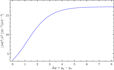
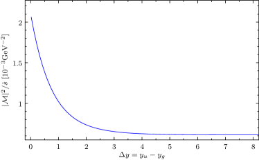
Figure 1: Regge scaling of quark-gluon scattering amplitudes in the MRK limit, approached by increasing $\Delta y$. Left: Rapidity ordering $qg\to qg$. Right: Rapidity ordering $qg\to gq$. The kinematics are fixed by the azimuthal angle $\phi_{1}=\frac{\pi}{7}$ and transverse momentum $p_{1\perp}=40\,$GeV of the outgoing particle in the backward direction.

2.2 $H+\geq 2j$ Processes within HEJ

The construction of the leading-logarithmic calculation of $pp\to H+\geq 2j$ in the HEJ framework was described in detail in [26, 17]. Here we summarise the main points in order to frame the discussion of the new components calculated in this paper.

Following the arguments in section 2.1, the LL configurations in pure QCD have the form $f_{a}f_{b}\to f_{a}\cdots f_{b}$, where $f_{a},f_{b}$ indicate the incoming parton flavours and the ellipsis denotes an arbitrary number of gluons. As before, the particles are written in order of increasing rapidity. The production of an additional Higgs boson proceeds via an effective coupling to two or more gluons. Since invariant masses are large in the high-energy region, it is crucial that the exact dependence on the top-quark mass is included in this effective coupling. A final-state Higgs boson with momentum $p_{H}\equiv p_{j}$ at an intermediate rapidity $y_{j}$ such that $y_{j-1}\ll y_{j}\ll y_{j+1}$ can then exchange $t$-channel gluons with the outgoing partons $j-1,j+1$. It was shown in [26] that the scaling behaviour in equation (2) directly generalises when a Higgs boson is emitted in the middle of the quarks and gluons. Therefore, all configurations $f_{a}f_{b}\to f_{a}\cdots H\cdots f_{b}$ contribute at LL accuracy.

In the MRK limit the amplitudes are found to factorise into a neat product of simple functions. In the High Energy Jets formalism we obtain the form

$$\begin{split}\overline{\left|\mathcal{M}_{{\tt HEJ}}^{f_{a}f_{b}\to f_{a}\cdots H\cdots f_{b}}\right|}^{2}={}&\mathcal{B}_{f_{a},H,f_{b}}(p_{a},p_{b},p_{1},p_{n},q_{j},q_{j+1})\\ &\cdot\prod_{\begin{subarray}{c}i=1\\ i\neq j\end{subarray}}^{n-2}\mathcal{V}(p_{a},p_{b},p_{1},p_{n},q_{i},q_{i+1})\\ &\cdot\prod_{i=1}^{n-1}\mathcal{W}(q_{i},y_{i},y_{i+1}),\end{split}$$ (3)

for the modulus square of the matrix element, summed and averaged over helicities and colours. In this expression, $p_{a}$ $(p_{b})$ is the incoming momentum in the backward (forward) direction and $p_{1},\dots,p_{n}$ are the outgoing momenta ordered in increasing rapidity. The $t$-channel momenta are given by

$$q_{1}=p_{a}-p_{1},\qquad q_{i}=q_{i-1}-p_{i}\;\text{ for }i>1.$$ (4)

The structure is illustrated in figure 2.

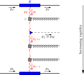
Figure 2: Structure of the matrix element for the process $f_{a}f_{b}\to f_{a}\cdots H\cdots f_{b}$.

At Born level, the right-hand side of equation (3) reduces to the function $\mathcal{B}_{f_{a},H,f_{b}}$, described below. $\mathcal{V}$ comprises the real corrections due to the production of $n-3$ gluons in addition to $f_{a},f_{b}$, and the Higgs boson. It is given by the contraction of two Lipatov vertices [26]:

$$\mathcal{V}(p_{a},p_{b},p_{1},p_{n},q_{i},q_{i+1})={} -\frac{C_{A}}{t_{i}t_{i+1}}V_{\mu}(p_{a},p_{b},p_{1},p_{n},q_{i},q_{i+1})V^{\mu}(p_{a},p_{b},p_{1},p_{n},q_{i},q_{i+1}),$$ (5)

$$V^{\mu}(p_{a},p_{b},p_{1},p_{n},q_{i},q_{i+1})={} -(q_{i}+q_{i+1})^{\mu}$$

$$+\frac{p_{a}^{\mu}}{2}\left(\frac{q_{i}^{2}}{p_{i+1}\cdot p_{a}}+\frac{p_{i+1}\cdot p_{b}}{p_{a}\cdot p_{b}}+\frac{p_{i+1}\cdot p_{n}}{p_{a}\cdot p_{n}}\right)+p_{a}\leftrightarrow p_{1}$$

$$-\frac{p_{b}^{\mu}}{2}\left(\frac{q_{i+1}^{2}}{p_{i+1}\cdot p_{b}}+\frac{p_{i+1}\cdot p_{a}}{p_{b}\cdot p_{a}}+\frac{p_{i+1}\cdot p_{1}}{p_{b}\cdot p_{1}}\right)-p_{b}\leftrightarrow p_{n},$$ (6)

where $t_{i}=q_{i}^{2}$ are the squares of the $t$-channel momenta. $\mathcal{W}$ accounts for the all-order finite contribution coming from the sum of the virtual corrections and unresolved real corrections. It is process-independent and described in detail in [26].

The process-dependent Born-level factor is given by

$$\mathcal{B}_{f_{a},H,f_{b}}=\frac{(4\pi\alpha_{s})^{n-1}}{4(N_{c}^{2}-1)}\frac{K_{f_{a}}(p_{1}^{-},p_{a}^{-})}{t_{1}}\ \frac{K_{f_{b}}(p_{n}^{+},p_{b}^{+})}{t_{n-1}}\frac{\left\|S_{f_{a}f_{b}\to f_{a}Hf_{b}}\right\|^{2}}{t_{j}t_{j+1}}.$$ (7)

Here, $\alpha_{s}$ is the strong coupling and $N_{c}=3$ is the number of colours. The difference between incoming gluons and (anti-)quarks is completely absorbed into the colour acceleration multipliers $K_{f}$ with

$$K_{g}(x,y)={} \frac{1}{2}\left(\frac{x}{y}+\frac{y}{x}\right)\left(C_{A}-\frac{1}{C_{A}}\right)+\frac{1}{C_{A}}$$ for gluons, (8)

$$K_{q}(x,y)={} C_{F}$$ for quarks and antiquarks. (9)

$C_{F}=\frac{N_{C}^{2}-1}{2N_{C}}$ and $C_{A}=N_{C}$ are the usual Casimir invariants. $S_{f_{a}f_{b}\to f_{a}Hf_{b}}$ is a contraction of currents with the Higgs boson production vertex. The double vertical bars indicate the sum over helicities of the corresponding amplitudes:

$$\left\|S_{f_{a}f_{b}\to f_{a}Hf_{b}}\right\|^{2}=\sum_{\begin{subarray}{c}\lambda_{a}=+,-\\ \lambda_{b}=+,-\end{subarray}}\left|j^{\lambda_{a}}_{\mu}(p_{1},p_{a})V_{H}^{\mu\nu}(q_{j},q_{j+1})j_{\nu}^{\lambda_{b}}(p_{n},p_{b})\right|^{2}.$$ (10)

$V_{H}$ is the well-known one-loop effective coupling between the Higgs boson and two gluons in the normalisation of [17], including the full quark-mass dependence. The inclusion of this piece in equation (3) then gives the correct finite quark-mass contributions at LL for any number of final state partons/jets. Finally, the current $j$ is given by

$$j^{\lambda}_{\mu}(p,q)=\bar{u}^{\lambda}(p)\gamma_{\mu}u^{\lambda}(q).$$ (11)

In addition to the LL resummation discussed so far, gauge-invariant subsets of next-to-leading logarithmic (NLL) corrections originating from non-FKL configurations have also been included in HEJ. One source of NLL corrections are the configurations $qf_{b}\to Hq\cdots f_{b}$ and $f_{a}q\to f_{a}\cdots qH$, which only permit $n-2$ $t$-channel gluon exchanges instead of the $n-1$ exchanges found in LL configurations. In these cases, we adapt the matrix element formula for the corresponding LL configurations to a flipped rapidity order of outgoing (anti-)quark and Higgs boson. If the Higgs boson is emitted first in rapidity order, we use equation (3) with $p_{2}\equiv p_{H}$ and exclude the virtual correction factor $\mathcal{W}$ for $i=1$. In the other case of the Higgs boson being emitted last, we set $p_{n-1}=p_{H}$ and skip $\mathcal{W}$ for $i=n-1$.

A second class of non-FKL configurations arises for three or more produced jets, when the most backward or forward outgoing particle is a gluon, but the corresponding incoming parton is a quark or antiquark. These “unordered gluon” configurations, $qf_{b}\to gq\cdots H\cdots f_{b}$ and $f_{a}q\to f_{a}\cdots H\cdots qg$, allow one $t$-channel gluon exchange less than the corresponding FKL configurations in which the unordered gluon is swapped with the neighbouring (anti-)quark. Hence, they contribute at NLL accuracy. Without loss of generality, we consider the case where the unordered gluon is the most backward emitted particle. We denote its momentum by $p_{g}$ and the following momenta by $p_{1},\dots,p_{n}$. The modulus square of the matrix element then has the same structure as in equation (3). In fact, the only changes are that the first $t$-channel momentum is now $q_{1}=p_{a}-p_{1}-p_{g}$ and that a different Born-level function $\mathcal{B}_{gq,H,f_{b}}$ depending also on $p_{g}$ appears. For a derivation and explicit expressions, see [26].

2.3 Scaling of $H+\geq 1j$ Amplitudes

To extend the formalism to the production of a Higgs boson with a single jet we first need to identify the LL configurations, following the discussion in section 2.1, and then derive the corresponding matrix elements.

So far, we have only considered LL configurations in which both the most backward and the most forward outgoing particle is a parton. However, in the process $gq\rightarrow Hq$, the amplitude should scale as $\mathcal{M}\sim s_{Hq}$, as there is a gluon exchange (thus a spin-1 particle) in the $t$-channel. Similarly, the process $gg\rightarrow Hg$ corresponds to $\mathcal{M}\sim s_{Hg}$. If we look at Higgs boson plus dijet production, the same argument allows us to establish that $gq\rightarrow Hgq$ scales as $\mathcal{M}\sim s_{Hg}s_{gq}$. All these configurations therefore contribute at LL accuracy. This is no longer the case if, for example, outgoing parton flavours are rearranged: $gq\rightarrow Hqg$ scales as $\mathcal{M}\sim s_{Hq}s_{qg}^{1/2}$.

Note that these scalings are valid whether we consider the full LO amplitude (with Higgs to gluons couplings via quark loops) or the Higgs Effective Field Theory (HEFT) one with an infinite top mass $m_{t}$, as shown in figure 3. To produce these plots, the amplitude is extracted from Madgraph5_aMC@NLO [27] and is calculated in a one-dimensional phase-space as a function of the rapidity separation between all pairs of particles. It was checked for consistency that setting the top mass to infinity in the LO amplitude yields the HEFT result. We compare to the LO truncation of the all-order HEJ amplitudes, anticipating their derivation from the high-energy limit in section 2.4,

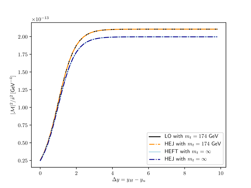
(a) $|\mathcal{M}|^{2}/\hat{s}^{2}$ for the process $gu\rightarrow Hu$

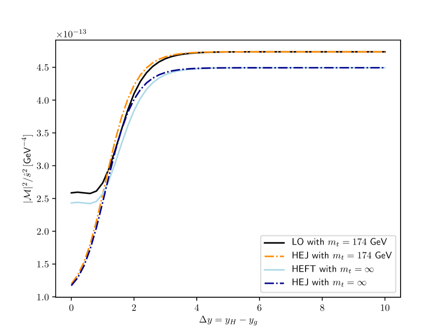
(b) $|\mathcal{M}|^{2}/\hat{s}^{2}$ for the process $gg\rightarrow Hg$

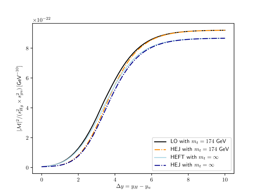
(c) $|\mathcal{M}|^{2}/(s_{Hg}^{2}\times s_{gu}^{2}))$ for the process $gu\rightarrow Hgu$

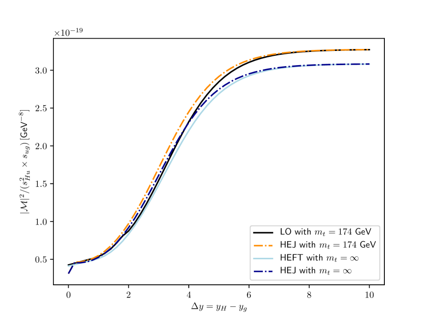
(d) $|\mathcal{M}|^{2}/(s_{Hu}^{2}\times s_{ug}))$ for the process $gu\rightarrow Hug$

Figure 3: Verifying Regge scaling of the squared matrix elements (equation (2)) for 4 different processes. Increasing values of $\Delta y$ on the $x$-axis approach the MRK limit (equation (1)).

The momentum configurations chosen are summarised in table 1. We stress though that the behaviour shown is not dependent on specific values of azimuthal angle or transverse momentum, but only on the rapidity assignment of the particles.

Process	Momenta configuration
$gq\rightarrow Hq$	$\begin{cases}y_{q}=-\Delta\text{ and }y_{H}=\Delta&\\ \phi_{q}=\frac{\pi}{4}&\\ p_{q\perp}=40\,\text{GeV}&\end{cases}$
$gg\rightarrow Hg$	$\begin{cases}y_{g}=-\Delta\text{ and }y_{H}=\Delta&\\ \phi_{g}=\frac{\pi}{4}&\\ p_{g\perp}=40\,\text{GeV}&\end{cases}$
$gq\rightarrow Hgq$	$\begin{cases}y_{q}=-\Delta,y_{g}=0\text{ and }y_{H}=\Delta&\\ \phi_{g}=\frac{\pi}{2}\text{ and }\phi_{q}=-\frac{\pi}{3}&\\ p_{g\perp}=k_{q\perp}=40\,\text{GeV}&\end{cases}$
$gq\rightarrow Hqg$	$\begin{cases}y_{g}=-\Delta,y_{q}=0\text{ and }y_{H}=\Delta&\\ \phi_{g}=-\frac{\pi}{2}\text{ and }\phi_{q}=\frac{\pi}{3}&\\ p_{g\perp}=k_{q\perp}=40\,\text{GeV}&\end{cases}$

Table 1: The momentum configurations used in figure 3.

2.4 New Components for $H+\geq 1j$ and an Outer Higgs Boson

In section 2.1 we discussed the factorisation of LL amplitudes for $f_{a}f_{b}\to f_{a}\cdots H\cdots f_{b}$ into a Born-level function $\mathcal{B}$, a product over real-emission vertices $\mathcal{V}$, and a product of virtual corrections $\mathcal{W}$. The same type of factorisation holds for LL configurations with the Higgs boson as the most forward or backward outgoing particle. In fact, the virtual corrections are the same as in equation (3). To derive the remaining factors, we first analyse the Born-level process $gf_{b}\to Hf_{b}$ and then consider real corrections.

2.4.1 Higgs Current

The Born-level function $\mathcal{B}_{H,f_{b}}$ for the process $gf_{b}\to H\cdots f_{b}$ is obtained by deriving a $t$-channel factorised form analogous to equation (7) from the modulus square of the Born-level amplitude in the MRK limit. For $gq\to Hq$, the tree-level amplitude is determined by a single diagram, depicted in figure 4.

Figure 4: The tree-level diagram for the process $gq\to Hq$. The straight solid line denotes an arbitrary light quark or antiquark.

Without requiring any approximations we obtain the factorised expression

$$\mathcal{B}_{H,f_{b}}={} \frac{(4\pi\alpha_{s})^{n-1}}{4(N_{c}^{2}-1)}\frac{1}{t_{1}}\frac{K_{f_{b}}(p_{n}^{+},p_{b}^{+})}{t_{n-1}}\left\|S_{gf_{b}\to Hf_{b}}\right\|^{2},$$ (12)

$$\left\|S_{gf_{b}\to Hf_{b}}\right\|^{2}={} \sum_{\begin{subarray}{c}\lambda_{a}=+,-\\ \lambda_{b}=+,-\end{subarray}}\left|\epsilon_{\mu}^{\lambda_{a}}(p_{a})\ V_{H}^{\mu\nu}(p_{a},p_{a}-p_{1})\ j_{\nu}^{\lambda_{b}}(p_{n},p_{b})\right|^{2},$$ (13)

for $f_{b}=q$, where $\epsilon^{\lambda_{a}}(p_{a})$ is the polarisation vector of the incoming gluon. This is plotted along with the exact LO results from Madgraph5_aMC@NLO [27] in figure 3(a), showing exact agreement for both finite top quark mass and in the infinite $m_{t}$ limit. In the MRK limit, this formula also holds for $f_{b}=g$, which is shown in figure 3(b). In this case there is some approximation away from the limit, but very quickly the LO and HEJ lines converge as $\Delta y$ increases.

2.4.2 Lipatov Vertex for Additional Gluons

In section 2.2, we described the simple factorised structure of amplitudes within (N)MRK limits. Not only are the different components independent of momenta in different parts of the chain, they are independent of the particle content of the rest of the chain. This should mean that the Lipatov vertex derived in pure QCD processes for additional gluons still applies. However, the Lorentz and colour structure of the “Higgs current” $j_{H}^{\nu}=\epsilon_{\mu}V_{H}^{\mu\nu}$ differ compared to pure QCD processes so it is important to check that this is indeed the case.

a)	b)	c)	d)

e)	f)	g)	h)

Figure 5: The eight LO diagrams which contribute to the process in equation (14).

We will consider the process

$$g(p_{a})q(p_{b})\rightarrow H(p_{1})g(p_{2})q(p_{3}),$$ (14)

in the MRK limit $y_{1}\ll y_{2}\ll y_{3}$. There are eight LO diagrams, as shown in fig. 5. Compact expressions for tree-level Higgs-plus-4 parton colour-ordered amplitudes appear in [28, 29]. Setting $q_{1}=p_{a}-p_{1}$ and $q_{2}=p_{3}-p_{b}$, the HEJ amplitude is given by

$$\begin{split}\mathcal{M}_{{\tt HEJ}}=ig_{s}^{2}f^{2ea}T^{e}_{3b}\ \frac{\bar{u}(p_{3})\gamma^{\nu}u(p_{b})}{q_{1}^{2}q_{2}^{2}}\ V^{\alpha}(p_{a},p_{b},p_{a},p_{3},q_{1},q_{2})V_{H}^{\mu\nu}(p_{a},q_{1})\ \varepsilon_{\mu}(p_{a})\varepsilon_{\alpha}(p_{2})^{*}.\end{split}$$ (15)

As the outer particle is no longer colour-charged, the third argument of the Lipatov vertex defined in equation (2.2) is now $p_{a}$ instead of $p_{1}$. The colour factor of the HEJ amplitude may be rewritten

$$if^{2ea}T^{e}_{3b}=(T^{a}T^{2})_{3b}-(T^{2}T^{a})_{3b}.$$ (16)

We can then directly compare equation (15) with the MRK limit of eqs. (26) and (27) in Ref. [29], and we find agreement at LL up to an unphysical phase arising from our spinor conventions. Specifically, the LL term in the MRK and infinite top-quark mass limit of equation (15) is given by

$$g_{s}^{2}\left(\frac{\alpha_{s}}{3\pi v}\right)if^{2ea}T^{e}_{3b}\frac{\langle 3a\rangle[ab]}{|p_{2\perp}||p_{3\perp}|}\rightarrow g_{s}^{2}\left(\frac{\alpha_{s}}{3\pi v}\right)if^{2ea}T^{e}_{3b}\frac{\hat{s}}{|p_{2\perp}||p_{3\perp}|},$$ (17)

where the angle and square brackets are Lorentz-invariant kinematic factors defined by $\langle ij\rangle=\bar{u}(p_{i})P_{R}u(p_{j})$ and $[ij]=\bar{u}(p_{i})P_{L}u(p_{j})$.

2.4.3 Matrix element including additional gluons

We can now use these results to form the analogue of equation (3) for the process $gf_{b}\to H\cdots f_{b}$

$$\begin{split}\overline{\left|\mathcal{M}_{{\tt HEJ}}^{gf_{b}\to H\cdots f_{b}}\right|}^{2}={}&\mathcal{B}_{H,f_{b}}(p_{a},p_{b},p_{1},p_{n})\\ &\cdot\prod_{i=1}^{n-2}\mathcal{V}(p_{a},p_{b},p_{a},p_{n},q_{i},q_{i+1})\\ &\cdot\prod_{i=1}^{n-1}\mathcal{W}(q_{i},y_{i},y_{i+1}),\end{split}$$ (18)

where the only differences to equation (3) are the Born-level function $\mathcal{B}_{H,f_{b}}(p_{a},p_{b},p_{1},p_{n})$ given in equation (12) and the third argument of the real-correction function $\mathcal{V}$. We illustrate that this gives the correct behaviour in the MRK limit in figure 3(c) for the processes $gu\to Hgu$, and in figure 3(d) we show that we obtain the correct limiting behaviour for the NLL configuration $gu\to Hug$.

3 Predictions and Comparison to Data

In this section we compare predictions for Higgs boson production in association with one or more jets obtained with High Energy Jets to those of fixed next-to-leading order perturbation theory and to experimental analyses. The analyses are implemented in Rivet [30] and relate to data collected at the LHC operated at both 13 TeV[31, 32] and 8 TeV [33].

3.1 Predictions

In our predictions, Sherpa [34] is used to generate leading-order events through Comix [35] and Openloops [36] for $H+n$ jets, where $n=1,\dots,5$. We include the exact dependence on the top-quark mass where available (i.e. for $n=1,2$) and for higher multiplicities use the simpler results valid for an infinite top mass. High-energy resummation is then applied using the method of HEJ 2, described in detail in [24]. This takes the fixed-order events as input and then adds all-order corrections (real and virtual) corresponding to each Born phase space point. The resulting resummation events are reweighted by

$$\frac{|{\cal M}_{\text{{\tt HEJ}}}(m_{t},m_{b})|^{2}}{|{\cal M}_{\text{{\tt HEJ}, LO}}(m_{t},0)|^{2}} \leq 2\text{ jets},$$ (19)

$$\frac{|{\cal M}_{\text{{\tt HEJ}}}(m_{t},m_{b})|^{2}}{|{\cal M}_{\text{{\tt HEJ}, LO}}(\infty,0)|^{2}} >2\text{ jets}.$$ (20)

${\cal M}_{\text{{\tt HEJ}}}(m_{t},m_{b})$ is the HEJ all-order matrix element discussed in section 2, where we have indicated the dependence on the top-quark mass $m_{t}$ and the bottom-quark mass $m_{b}$. ${\cal M}_{\text{{\tt HEJ}, LO}}(m_{t},m_{b})$ denotes the leading-order truncation of the HEJ matrix element. The $p_{T}$-sampling for the leading-order events used for the matching extends slightly beyond the cuts used in the analysis, as required by the mapping between the high-multiplicity $m$-body resummation phase space point and the $n$-parton ($n<m$) phase space point of the matching. One way to look at this is that the radiation produced by the resummation on top of the fixed-order input modifies the momenta in the input, and the over-sampling is needed in order for the full analysis-phase space of the resummation events to be covered.

We also use Sherpa and Openloops to provide NLO 1-jet and 2-jet predictions in the infinite top-quark mass limit without resummation, for comparisons with HEJ and the experimental data. The cross sections presented from HEJ are further matched to NLO by multiplying the predictions for the inclusive 1-jet (or 2-jet) distributions by the ratio of the inclusive 1-jet (resp. 2-jet) cross-section at NLO divided by the inclusive 1-jet (resp. 2-jet) cross-section of HEJ expanded to NLO. This changes the normalisation of distributions, and reduces the scale variation.

$$\frac{d\sigma_{\text{HEJNLO}n\text{J}}}{d\mathcal{O}}={} \frac{\sigma_{\text{NLO}n\text{J}}}{\sigma_{\text{{\tt HEJ}}n\text{J}}}\frac{d\sigma_{\text{{\tt HEJ}}}}{d\mathcal{O}},$$ (21)

where $\sigma_{\text{NLO}n\text{J}},n=1,2$ denotes the inclusive $n$-jet cross section at NLO and $\sigma_{\text{{\tt HEJ}}n\text{J}}$ the HEJ prediction for the inclusive $n$-jet cross section. Note that the components of the cross section with exclusive three or more jets as predicted by HEJ are technically matched only at Born level, but since they form part of the inclusive one or two-jet observables, their contribution is scaled by the relevant ratio in eq. (21).

We use the NNPDF30@NNLO [37] PDF set provided from the LHAPDF collaboration [38] for HEJ and NLO predictions, with the central scale choice $\mu_{F}=\mu_{R}=\max(m_{12},m_{H})$ (where $m_{12}$ is the invariant mass between the two hardest jets, and set to $m_{12}=0$ for 1-jet events). In order to gauge the scale dependence of the predictions the scales are varied independently by a conventional factor of two, excluding combinations where $\mu_{F}$ and $\mu_{R}$ differ by a factor of more than two. The coloured regions in the figures below indicate the theoretical uncertainty envelope formed by these scale variations.

We also investigated an alternative central scale choice $\mu_{F}=\mu_{R}=H_{T}/2$. The predictions changed only minimally with this scale compared to the custom scale choice above and so are not presented in this study.

3.2 Predictions for 13 TeV and Comparison to Data

In this section we present predictions for a CMS analysis [31, 32] at a centre-of-mass energy of $\sqrt{\hat{s}}=13$ TeV and for additional distributions showcasing differences between HEJ and fixed order predictions at NLO. The CMS study explored distributions for Higgs boson production (and decay in the di-photon channel) both inclusively and in association with one jet.

The baseline cuts related to the photons and the jets are listed in table 2 (see refs. [31, 32] for a full discussion). The pseudo-rapidity jet cuts are specific to the observables studied and are listed in table 3. Jets are reconstructed with the anti-$k_{T}$ [39] jet algorithm with $R=0.4$.

Description	Baseline cuts
Leading photon transverse momentum	$p_{T}(\gamma_{1})>30\text{ GeV}$
Subleading photon transverse momentum	$p_{T}(\gamma_{2})>18\text{ GeV}$
Diphoton invariant mass	$m_{\gamma\gamma}>90\text{ GeV}$
Pseudo-rapidity of the photons	$|\eta_{\gamma}|<2.5$
	excluding $1.4442<|\eta_{\gamma}|<1.566$
Ratio of harder photon $p_{T}$ to diphoton invariant mass	$p_{T}(\gamma_{1})/m_{\gamma\gamma}>\frac{1}{3}$
Ratio of softer photon $p_{T}$ to diphoton invariant mass	$p_{T}(\gamma_{2})/m_{\gamma\gamma}>\frac{1}{4}$
Photon isolation cut	$\text{Iso}^{\gamma}_{\text{gen}}<10\text{ GeV}$
Jet transverse momentum	$p_{T}(j)>30\text{ GeV}$

Table 2: Baseline photon and jet cuts of the 13 TeV analysis, following the CMS analysis of [31, 32]. $\text{Iso}^{\gamma}_{\text{gen}}$ denotes the sum of transverse energies of stable particles in a cone of radius $\Delta R$ = 0.3 around each photon.

Observable	Pseudo-rapidity jet cut
Number of jets $N_{\text{jets}}$, figure 6(a)	$|\eta_{j}|<2.5$ (all jets)
$|p_{T}^{j_{1}}|$, figure 6(b)	$|\eta_{j_{1}}|<2.5$ (hardest jet) and $|\eta_{j}|<4.7$ (other jets)
$\min m_{ff}$, figure 7(a)	$|\eta_{j_{1}}|<2.5$ (hardest jet) and $|\eta_{j}|<4.7$ (other jets)
$\max m_{ff}$, figure 7(b)	$|\eta_{j_{1}}|<2.5$ (hardest jet) and $|\eta_{j}|<4.7$ (other jets)

Table 3: Pseudo-rapidity jet cuts used for the 13 TeV analysis observables presented in this section, following the CMS analysis of [31, 32].

The HEJ and NLO QCD predictions only describe $pp\to H+n$-jet processes via gluon fusion (GF) where the jets consist of light quarks and gluons. The data includes a non-GF contribution from electroweak VBF, $VH$ and $t\bar{t}H$ processes, labelled together as $HX$ in the experimental papers. We have extracted the value of this component from the experimental papers for the rest of this section, and added it to both the HEJ and NLO QCD predictions, where possible. This is indicated with “+HX” in the legend.

Figure 6(a) shows the exclusive number of jets where the 1-jet and 2-jet HEJ predictions are rescaled as described in equation (21). The fixed-order predictions are limited to 2 jets at NLO and 3 jets at LO, whereas HEJ allows us to make predictions for the $\geq 4$-jet bin and reasonable agreement is achieved throughout.

In figure 6(b), the transverse momentum of the first jet is shown. We have compared to data from [31] here rather than [32] as it covers a larger range. The discrepancy between NLO and HEJ predictions as the transverse momentum increases is due to the resummation procedure, and has also been observed in $W$+jets processes (see ref. [40]). The effect would be even more significant for greater values of $p_{T}$, however the collected data does not probe this region of phase-space. We have previously observed that a similar harder $p_{T}$-spectrum seen in $H+\geq 2j$ processes in HEJ leads to a greater sensitivity to the effects of using finite top and bottom quark masses [17].

The minimum rapidity separation between any two particles in the final state is shown in figure 7(a). As the Higgs boson is one of these final states, this is a 1-jet observable, so the NLO 1-jet predictions are shown for comparison and the HEJ predictions are scaled by the ratio of the NLO to HEJ inclusive 1-jet rates. This observable is very sensitive to high-energy logarithmic corrections, and as was observed in previous studies (see ref. [17]), the effect of the resummation results in a significant lowering of the HEJ prediction compared to fixed-order, by as much as 50% at large values. Figure 7(b) shows the maximum invariant mass between any two particles in the final state. This is related to the high energy limit where all pairwise invariant masses are taken to be large, but also includes situations where two or more particles have a small invariant mass. The impact of the logarithmic corrections is not as strong here, and the fixed-order and resummed predictions agree within uncertainties.

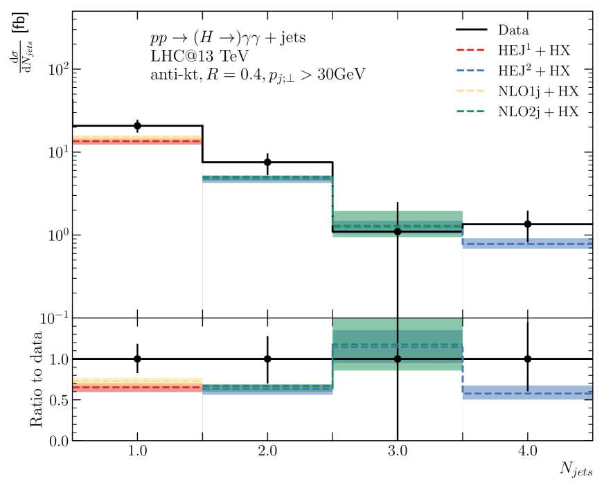
(a)

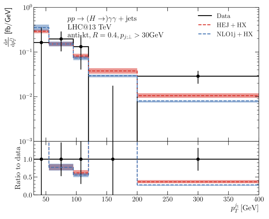
(b)

Figure 6: (a) The exclusive number of jets compared to CMS data from [32], and (b) the transverse momentum distribution of the leading jet compared to CMS data [31]. Both analyses employ the cuts described in table 2. The “HX” component is extracted from those publications.

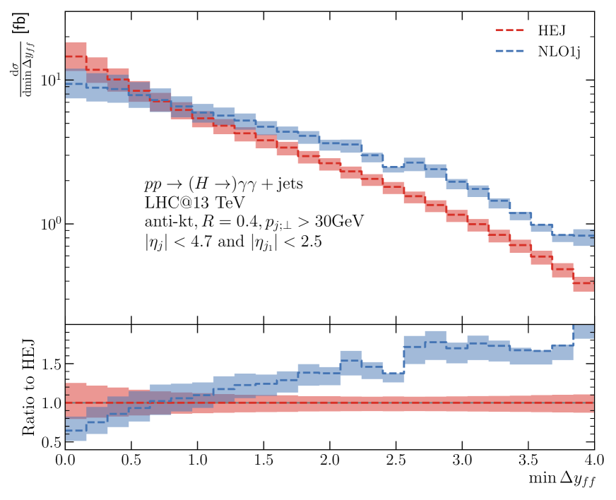
(a)

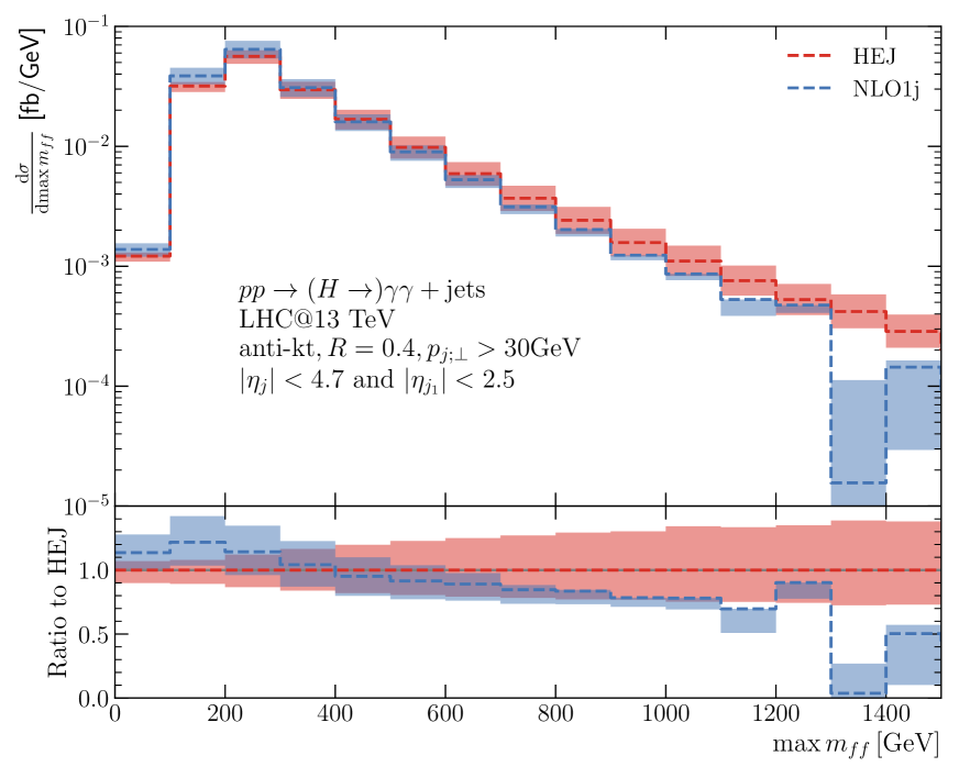
(b)

Figure 7: High-energy sensitive inclusive 1-jet distributions: (a) the minimum rapidity separation between any two outgoing particles (Higgs boson or jets) and (b) the maximum invariant mass between any two outgoing particles (Higgs or jets). HEJ results are rescaled by the inclusive cross section ratio $\sigma_{\text{NLO1J}}/\sigma_{\text{{\tt HEJ} 1J}}$.

3.3 Predictions for 8 TeV and Comparison to Data

We now present predictions for an ATLAS analysis [33] at a centre-of-mass energy of $\sqrt{\hat{s}}=8$ TeV as implemented in Rivet[30]. We list the relevant experimental cuts used in this analysis in table 4, the complete list being available in the experimental publication. As in the experimental analysis, the jets are reconstructed with the anti-$k_{T}$ algorithm with a radius parameter of $R=0.4$. This study explored the inclusive and differential cross-sections for Higgs boson production in the diphoton decay channel. For our purposes, we select the observables which correspond to Higgs boson production plus at least one jet, where our predictions are applicable.

Description	Baseline cuts
Photon transverse momentum	$p_{T}(\gamma)>25\text{ GeV}$
Diphoton invariant mass	$105\text{ GeV}<m_{\gamma\gamma}<160\text{ GeV}$
Pseudo-rapidity of the photons	$|\eta_{\gamma}|<2.37$ excluding $1.37<|\eta_{\gamma}|<1.56$
Ratio of harder photon $p_{T}$ to diphoton invariant mass	$p_{T}(\gamma_{1})/m_{\gamma\gamma}>0.35$
Ratio of softer photon $p_{T}$ to diphoton invariant mass	$p_{T}(\gamma_{2})/m_{\gamma\gamma}>0.25$
Photon isolation cut	$\text{Iso}^{\gamma}_{\text{gen}}<14\text{ GeV}$
Jet transverse momentum	$p_{T}(j)>30\text{ GeV}$
Jet rapidity	$|y_{j}|<4.4$

Table 4: Baseline cuts of the 8 TeV analysis, following the ATLAS analysis of [33]. $\text{Iso}^{\gamma}_{\text{gen}}$ denotes the sum of transverse energies of stable particles in a cone of radius $\Delta R$ = 0.4 around each photon.

We divide our results into 1-jet observables, i.e. containing at least one jet, where the new components of HEJ as detailed in section 2.3 can be tested, and 2-jet observables. As in the previous subsection, the experimental data points here include a non-GF contribution. We have extracted this “HX” component from [33] where this was available.

3.3.1 $H+\geq 1j$

In figure 8(a), we show the exclusive number of jets. As was evidenced at 13 TeV, the differences between fixed-order and resummed predictions are limited after the inclusive cross sections are rescaled. The NLO and HEJ predictions for the 1- and 2-jet rates are such that the bands for the theoretical scale variance and data uncertainty bands overlap. The predictions in the $\geq 3$-jet bin remain slightly below data.

In figure 8(b), the rapidity of the leading jet is displayed: the discrepancy between the fixed-order and the resummed predictions increases as the rapidity of the jet attains large values. This is a High-Energy effect as opposed to a finite quark mass effect. Indeed, the corrections in $\hat{s}/t$ are particularly sizeable in this region of phase-space, and previous studies (see. ref [17]) showed little dependence on the inclusion of the finite quark mass effects on this observable. However, this is not the case for the transverse momentum of the Higgs boson of figure 8(c). The finite quark mass effects and the resummation lead to a hardening of the high-$p_{T}$ tail of the Higgs boson, which would be even more dramatic had that region been probed. Due to the probed phase-space region of $p_{T}<140\,\text{GeV}$, HEJ and fixed-order predictions for the hardest jet transverse momentum of figure 8(d) remain close together and difficult to disentangle.

The High-Energy sensitive observables of figure 9 behave in a similar fashion to those at 13 TeV (figure 7) for the reasons explained in section 3.2. Here, there is nearly a factor of two difference between NLO and HEJ at large values of min $\Delta y_{ff}$.

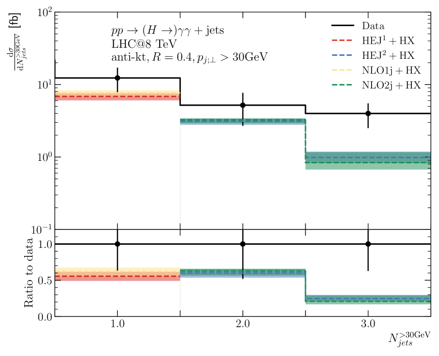
(a) Number of jets

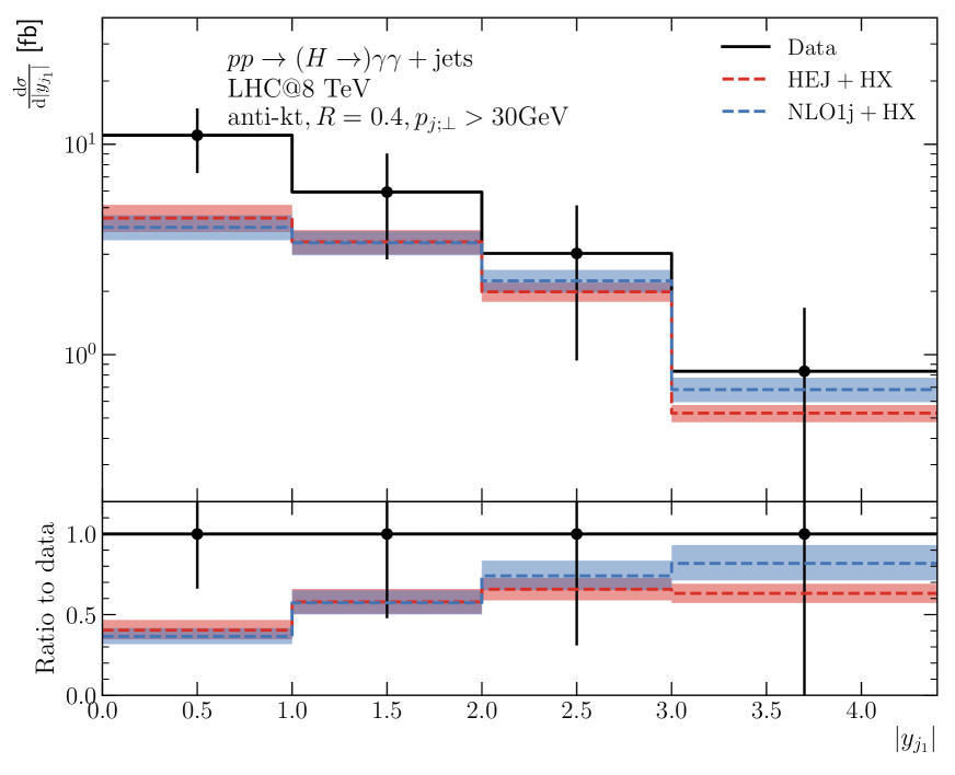
(b) Leading jet rapidity

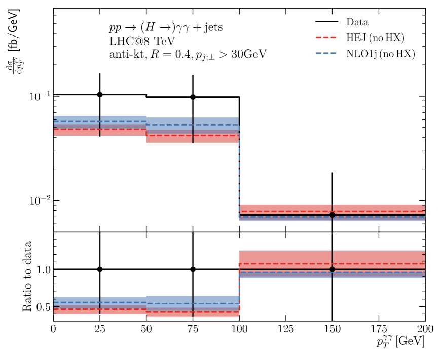
(c) $p_{T}$ of the Higgs boson, $N_{\text{jets}}=1$

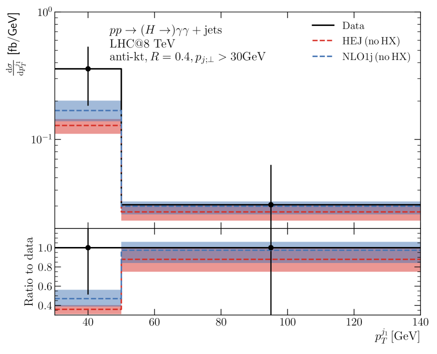
(d) Leading jet $p_{T}$, $N_{\text{jets}}=1$

Figure 8: (8(a)): Number of jets (exclusive). (8(b)): Leading jet rapidity. (8(c)): Higgs boson transverse momentum in the 1-jet bin. (8(d)): Leading jet transverse momentum in the 1-jet bin. The 1-jet HEJ predictions are rescaled by the inclusive cross section ratio $\sigma_{\text{NLO1J}}/\sigma_{\text{{\tt HEJ} 1J}}$ while the HEJ predictions of the 2 and 3-jet bins of (8(a)) are rescaled by $\sigma_{\text{NLO2J}}/\sigma_{\text{{\tt HEJ} 2J}}$. In (8(a)) and (8(b)), the “HX” component is extracted from [33]; this was not available for (8(c)) and (8(d)).

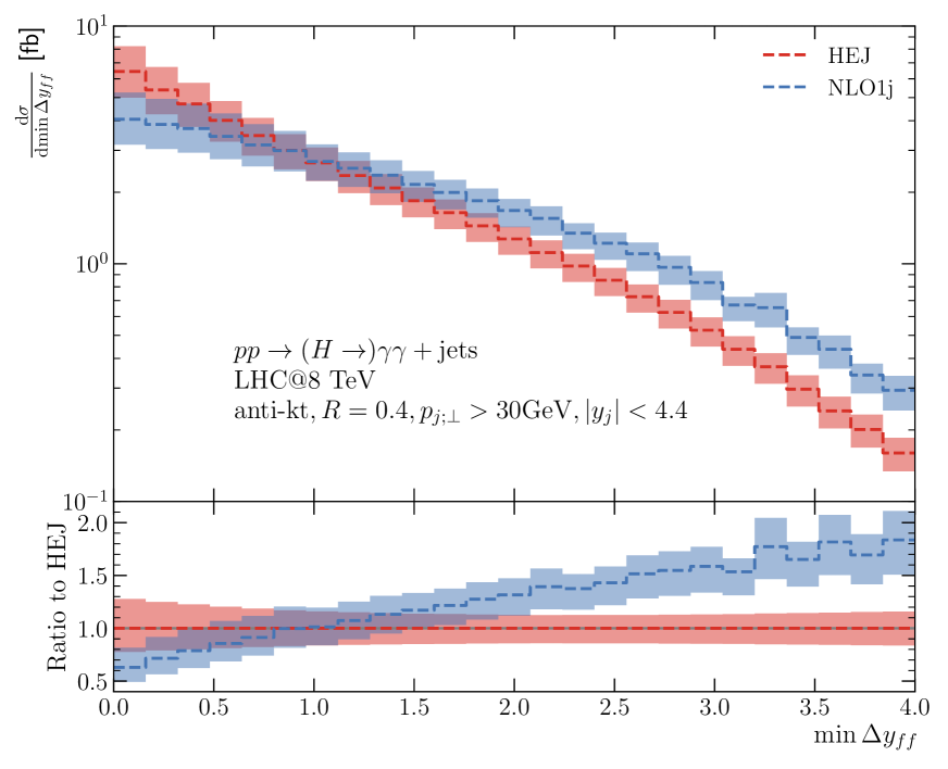
(a) $\text{min }\Delta y_{ff}$

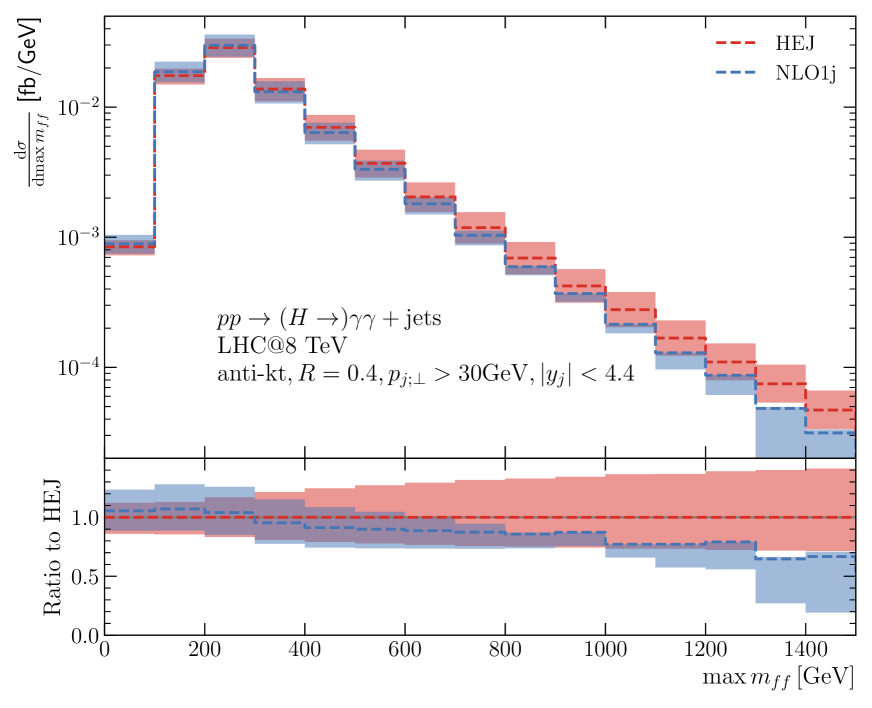
(b) $\text{max }m_{ff}$

Figure 9: High-energy sensitive 1-jet distributions. (9(a)): minimum rapidity separation between any two outgoing particles (Higgs boson or jets). (9(b)): maximum invariant mass between any two outgoing particles (Higgs boson or jets). HEJ results are rescaled by the inclusive cross section ratio $\sigma_{\text{NLO1J}}/\sigma_{\text{{\tt HEJ} 1J}}$.

3.3.2 $H+\geq 2j$

We now turn to a range of 2-jet observables, displayed in figures 10 and 11. Globally, the impact of the resummation on High-Energy sensitive observables is to lower the predictions from fixed-order approaches, as can be seen in large dijet rapidity separation in figure 10(a), large rapidity values of the second hardest jet in figure 10(b) and at large dijet invariant mass in figure 10(c). This can be seen more clearly before the addition of the “HX” component, see figure 12(a) in appendix B. As expected, the resummation procedure has little impact on the observables dependent on the azimuthal degrees of freedom: the azimuthal angle difference between the leading two jets of figure 10(d) and the azimuthal angle difference between the diphoton and the leading dijets systems depicted in figure 11(a), expect perhaps at values close to $\pi$ (that is when the systems are back-to-back).

As previously observed, the combination of the inclusion of corrections in $\hat{s}/t$ and the finite quark mass effects tend to harden the tail of the transverse momenta distributions compared to fixed order predictions. This is apparent in the description of the third-leading jet transverse momentum of figure 11(b) (see figure 12(b) for the shapes of the pure QCD predictions), but also in the transverse momentum of the diphoton-dijet system of figure 11(c). Although the Higgs transverse momentum seems to be independent of the effect of the resummation, it is conjectured that values of $p^{\gamma\gamma}_{\perp}$ above 200 GeV would lead to a disparity between the two approaches.

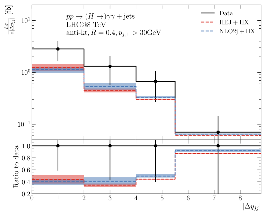
(a) Dijet rapidity separation

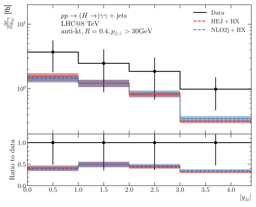
(b) Subleading jet rapidity

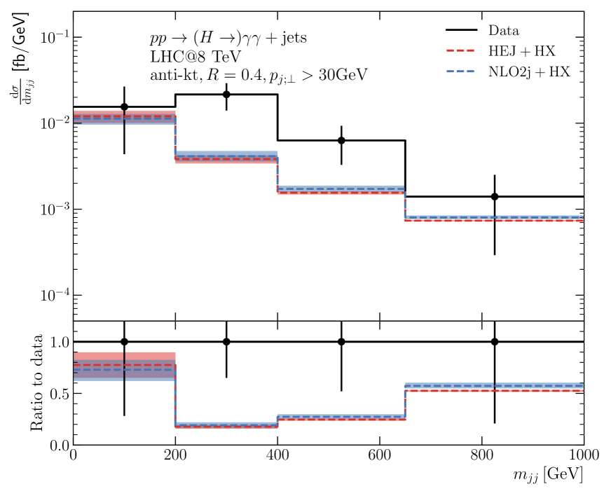
(c) Invariant dijet mass

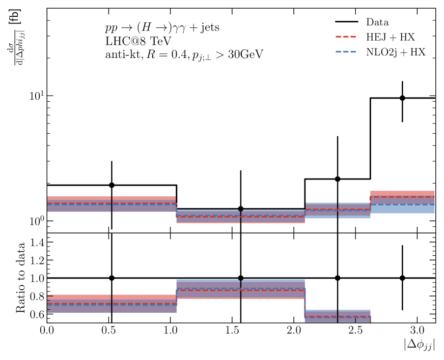
(d) $\Delta\phi$ between the leading 2 jets

Figure 10: (10(a)): Dijet rapidity separation. (10(b)): Subleading jet rapidity. (10(c)): dijet invariant mass. (10(d)): Azimuthal angle difference between the leading 2 jets. All 2-jet HEJ predictions are rescaled by the inclusive cross section ratio $\sigma_{\text{NLO2J}}/\sigma_{\text{{\tt HEJ} 2J}}$. The “HX” component is extracted from [33].

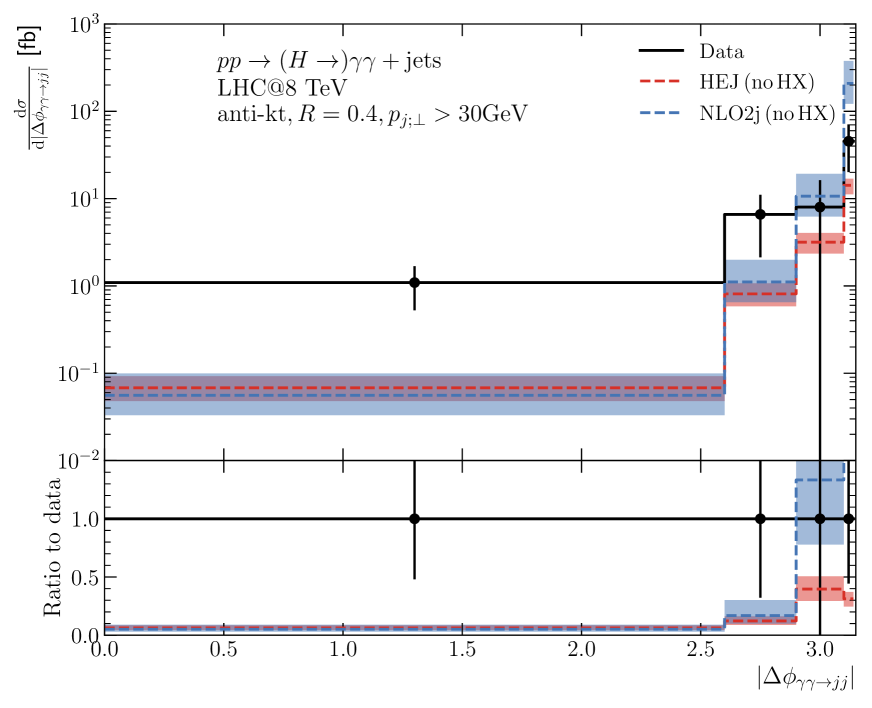
(a) $\Delta\phi$ between dijet and diphoton systems

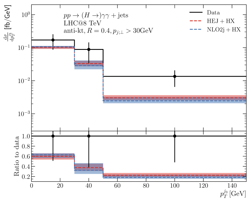
(b) Third-leading jet $p_{T}$

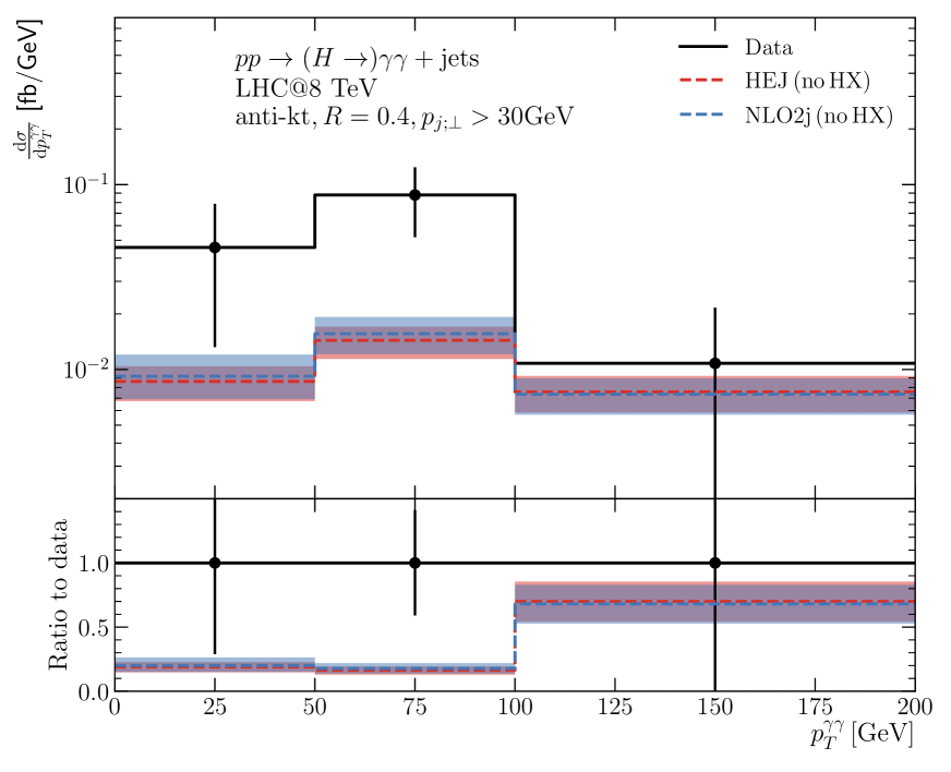
(c) Higgs $p_{T}$ with $N_{\text{jets}}=2$

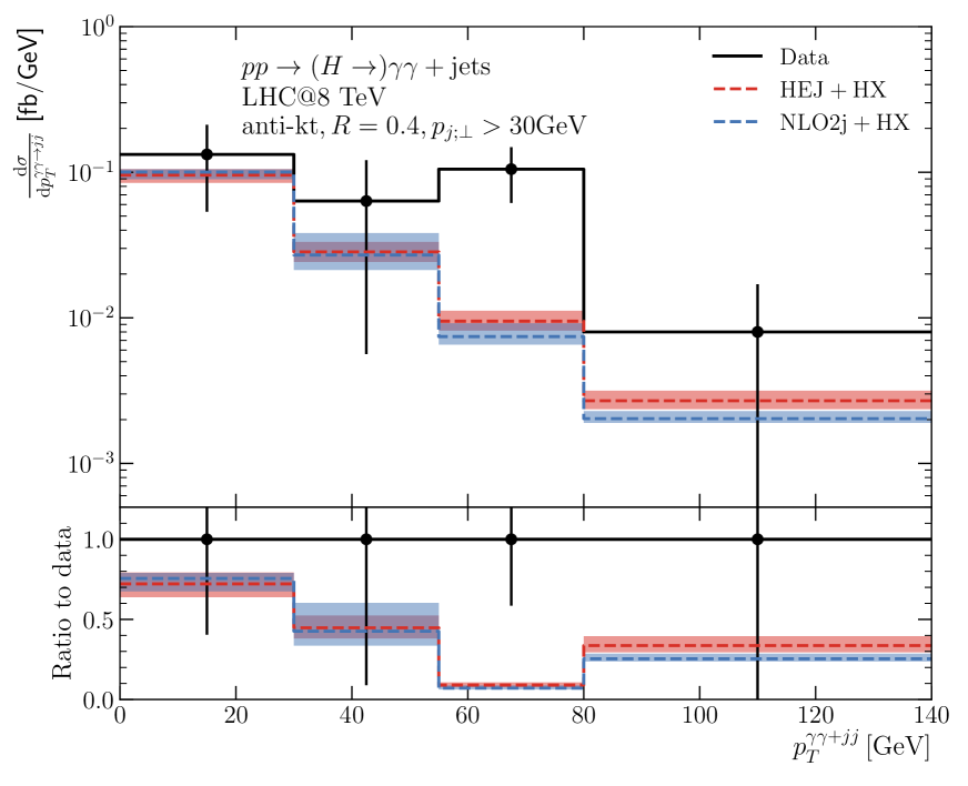
(d) $p_{T}$ of diphoton-dijet system

Figure 11: (11(a)): Azimuthal angle difference between dijet and diphoton objects. (11(b)): Transverse momentum of the third-leading jet. (11(c)): Transverse momentum of the Higgs boson in the $\geq$ 2-jet bin. (11(d)): Transverse momentum of the Higgs plus dijet object : $(p_{H}+p_{j_{1}}+p_{j_{2}})_{\perp}$. All 2 and 3-jet HEJ predictions are rescaled by the inclusive cross section ratio $\sigma_{\text{NLO2J}}/\sigma_{\text{{\tt HEJ} 2J}}$. In (11(b)) and (11(d)), the “HX” component is extracted from [33]; this was not available for (11(a)) and (11(c)).

4 Conclusions

In this paper we have presented an alternative description of $pp\to H+\geq 1j$, which is accurate to leading logarithms in $\hat{s}/p_{T}^{2}$ (LL). We have outlined the structure of a LL-accurate amplitude in the HEJ formalism, and described the calculation of the necessary new components in section 2. One big advantage of the approach is that it maintains full dependence on the finite top and bottom quark masses in the couplings of the Higgs boson to gluons for any number of jets, which quickly exceeds the multiplicities currently calculated at even leading order. The new pieces allow LL resummation in $\hat{s}/p_{T}^{2}$ to an inclusive 1-jet process for the first time in the HEJ framework.

We have then compared the resummed predictions to fixed-order predictions and to LHC data in section 3, and discussed the impact of the logarithmic corrections. We find the impact of the resummation is seen at large jet transverse momenta. The resummed results give a harder $p_{T}$-spectrum compared to NLO, which in turn leads to a greater dependence on finite quark masses in the coupling. We also observe a large suppression compared to NLO at large values of rapidity separation between all pairs of final state particles (i.e. between any two of the Higgs boson and jets). This can be as much of a factor of two and lies significantly outwith the uncertainty bands on the two predictions. Other observables, e.g. azimuthal angles, are less sensitive to these logarithmic corrections.

Looking forward to analyses of LHC Run 3 data, our results suggest that the inclusion of finite quark masses for higher jet multiplicities and of logarithmic corrections in $\hat{s}/p_{T}^{2}$ will be important in the comparison to data.

Appendix A NLO reweighting factors

In table 5, we give the value of the NLO reweighting factors as described in equation (21) for both the 8 TeV [33] and 13 TeV [31, 32] analyses.

Analysis	8 TeV			13 TeV
Scale	$\mu_{F},\mu_{R}$	$(\mu_{F},\mu_{R})/2$	$2(\mu_{F},\mu_{R})$	$\mu_{F},\mu_{R}$	$(\mu_{F},\mu_{R})/2$	$2(\mu_{F},\mu_{R})$
1J factor	1.87	1.54	2.15	1.59	1.30	1.84
2J factor	1.98	1.48	2.40	1.62	1.19	2.00

Table 5: NLO Reweighting factors with $\mu_{F}=\mu_{R}=\max(m_{12},m_{H})$.

In the 8 TeV analysis, the inclusive 1-jet and 2-jet cross-sections are calculated from the rapidity of the hardest and second hardest jet histograms respectively, figures 8(b) and 10(b).

In the 13 TeV analysis, the inclusive 1-jet and 2-jet cross-sections are obtained from the appropriate $N_{\text{jets}}$ bins, figure 6(a). Note that for at least 2 jets, this plot requires central jets only, but it is valid to use it as it is the only plot we present for the 2-jet observables. If more inclusive cross-sections are considered, say from the rapidity of the second hardest jet histogram over all the experimental range, then the 2-jet reweighting factor would be further away from the 1-jet value (1.79 for the central scale instead of 1.62).

Appendix B Additional Plots of QCD Component

In section 3, we showed the predictions from HEJ and at NLO compared to LHC data at 8 and 13 TeV. In order to make a realistic comparison, we have added the “HX” component from the experimental papers. Here, we include a few examples where the difference in shape resulting from the all-order QCD treatment in HEJ can be more clearly seen by studying only the QCD component. Figure 12 shows this for two distributions (originally shown in figures 10(a) and 11(b)). Here we can see that the HEJ predictions are strongly suppressed compared to NLO as rapidity separation increases (figure 12(a)); however the transverse momentum spectrum is harder for the third jet (figure 12(b)).

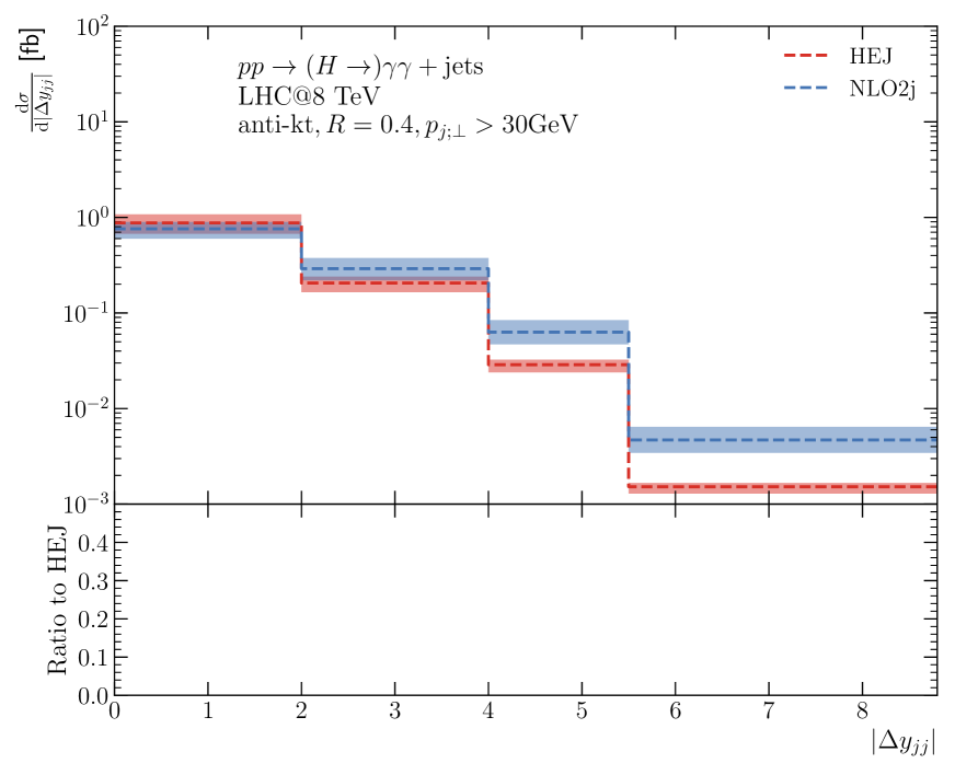
(a) Dijet rapidity separation

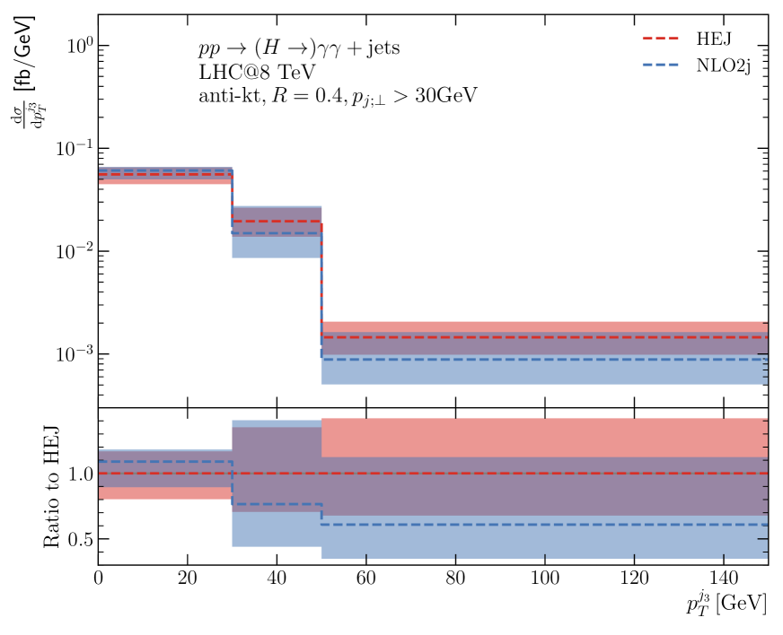
(b) Subleading jet rapidity

Figure 12: (12(a)): Dijet rapidity separation. (10(d)): Azimuthal angle difference between the leading 2 jets. This shows the distributions from Figs. 10(a) and 11(b), where now we only show the QCD contribution. As before, the 2-jet HEJ predictions are rescaled by the inclusive cross section ratio $\sigma_{\text{NLO2J}}/\sigma_{\text{{\tt HEJ} 2J}}$.

References

- [1] M. Czakon, R. V. Harlander, J. Klappert and M. Niggetiedt, Exact Top-Quark Mass Dependence in Hadronic Higgs Production, Phys. Rev. Lett. 127 (2021) 162002, [2105.04436].
- [2] S. P. Jones, M. Kerner and G. Luisoni, Next-to-Leading-Order QCD Corrections to Higgs Boson Plus Jet Production with Full Top-Quark Mass Dependence, Phys. Rev. Lett. 120 (2018) 162001, [1802.00349].
- [3] X. Chen, A. Huss, S. P. Jones, M. Kerner, J. N. Lang, J. M. Lindert et al., Top-quark mass effects in H+jet and H+2 jets production, JHEP 03 (2022) 096, [2110.06953].
- [4] V. Del Duca, W. Kilgore, C. Oleari, C. Schmidt and D. Zeppenfeld, Higgs + 2 jets via gluon fusion, Phys. Rev. Lett. 87 (2001) 122001, [hep-ph/0105129].
- [5] V. Del Duca, W. Kilgore, C. Oleari, C. Schmidt and D. Zeppenfeld, Gluon fusion contributions to H + 2 jet production, Nucl. Phys. B 616 (2001) 367–399, [hep-ph/0108030].
- [6] C. Anastasiou, C. Duhr, F. Dulat, F. Herzog and B. Mistlberger, Higgs Boson Gluon-Fusion Production in QCD at Three Loops, Phys. Rev. Lett. 114 (2015) 212001, [1503.06056].
- [7] F. Dulat, B. Mistlberger and A. Pelloni, Differential Higgs production at N3LO beyond threshold, JHEP 01 (2018) 145, [1710.03016].
- [8] B. Mistlberger, Higgs boson production at hadron colliders at N3LO in QCD, JHEP 05 (2018) 028, [1802.00833].
- [9] L. Cieri, X. Chen, T. Gehrmann, E. W. N. Glover and A. Huss, Higgs boson production at the LHC using the subtraction formalism at N3LO QCD, JHEP 02 (2019) 096, [1807.11501].
- [10] X. Chen, T. Gehrmann, E. W. N. Glover, A. Huss, B. Mistlberger and A. Pelloni, Fully Differential Higgs Boson Production to Third Order in QCD, Phys. Rev. Lett. 127 (2021) 072002, [2102.07607].
- [11] R. Boughezal, F. Caola, K. Melnikov, F. Petriello and M. Schulze, Higgs boson production in association with a jet at next-to-next-to-leading order in perturbative QCD, JHEP 06 (2013) 072, [1302.6216].
- [12] X. Chen, T. Gehrmann, E. W. N. Glover and M. Jaquier, Precise QCD predictions for the production of Higgs + jet final states, Phys. Lett. B 740 (2015) 147–150, [1408.5325].
- [13] R. Boughezal, F. Caola, K. Melnikov, F. Petriello and M. Schulze, Higgs boson production in association with a jet at next-to-next-to-leading order, Phys. Rev. Lett. 115 (2015) 082003, [1504.07922].
- [14] J. M. Campbell, R. K. Ellis and G. Zanderighi, Next-to-Leading order Higgs + 2 jet production via gluon fusion, JHEP 10 (2006) 028, [hep-ph/0608194].
- [15] J. M. Campbell, R. K. Ellis and C. Williams, Hadronic Production of a Higgs Boson and Two Jets at Next-to-Leading Order, Phys. Rev. D 81 (2010) 074023, [1001.4495].
- [16] V. Del Duca, W. Kilgore, C. Oleari, C. R. Schmidt and D. Zeppenfeld, Kinematical limits on Higgs boson production via gluon fusion in association with jets, Phys. Rev. D 67 (2003) 073003, [hep-ph/0301013].
- [17] J. R. Andersen, J. D. Cockburn, M. Heil, A. Maier and J. M. Smillie, Finite Quark-Mass Effects in Higgs Boson Production with Dijets at Large Energies, JHEP 04 (2019) 127, [1812.08072].
- [18] A. H. Mueller and H. Navelet, An Inclusive Minijet Cross-Section and the Bare Pomeron in QCD, Nucl. Phys. B 282 (1987) 727–744.
- [19] B.-W. Xiao and F. Yuan, BFKL and Sudakov Resummation in Higgs Boson Plus Jet Production with Large Rapidity Separation, Phys. Lett. B 782 (2018) 28–33, [1801.05478].
- [20] F. G. Celiberto, D. Y. Ivanov, M. M. A. Mohammed and A. Papa, High-energy resummed distributions for the inclusive Higgs-plus-jet production at the LHC, Eur. Phys. J. C 81 (2021) 293, [2008.00501].
- [21] J. R. Andersen and J. M. Smillie, Constructing All-Order Corrections to Multi-Jet Rates, JHEP 1001 (2010) 039, [0908.2786].
- [22] J. R. Andersen and J. M. Smillie, The Factorisation of the t-channel Pole in Quark-Gluon Scattering, Phys.Rev. D81 (2010) 114021, [0910.5113].
- [23] J. R. Andersen and J. M. Smillie, Multiple Jets at the LHC with High Energy Jets, JHEP 1106 (2011) 010, [1101.5394].
- [24] J. R. Andersen, T. Hapola, M. Heil, A. Maier and J. M. Smillie, Higgs-boson plus Dijets: Higher-Order Matching for High-Energy Predictions, JHEP 08 (2018) 090, [1805.04446].
- [25] V. S. Fadin, R. Fiore, M. G. Kozlov and A. V. Reznichenko, Proof of the multi-Regge form of QCD amplitudes with gluon exchanges in the NLA, Phys. Lett. B 639 (2006) 74–81, [hep-ph/0602006].
- [26] J. R. Andersen, T. Hapola, A. Maier and J. M. Smillie, Higgs Boson Plus Dijets: Higher Order Corrections, JHEP 09 (2017) 065, [1706.01002].
- [27] J. Alwall, R. Frederix, S. Frixione, V. Hirschi, F. Maltoni, O. Mattelaer et al., The automated computation of tree-level and next-to-leading order differential cross sections, and their matching to parton shower simulations, JHEP 07 (2014) 079, [1405.0301].
- [28] S. Dawson and R. P. Kauffman, Higgs boson plus multi - jet rates at the SSC, Phys. Rev. Lett. 68 (1992) 2273–2276.
- [29] R. P. Kauffman, S. V. Desai and D. Risal, Production of a Higgs boson plus two jets in hadronic collisions, Phys. Rev. D 55 (1997) 4005–4015, [hep-ph/9610541].
- [30] C. Bierlich et al., Robust Independent Validation of Experiment and Theory: Rivet version 3, SciPost Phys. 8 (2020) 026, [1912.05451].
- [31] CMS collaboration, A. M. Sirunyan et al., Measurement of inclusive and differential Higgs boson production cross sections in the diphoton decay channel in proton-proton collisions at 13 TeV, JHEP 01 (2019) 183, [1807.03825].
- [32] CMS collaboration, Measurement of the Higgs boson inclusive and differential fiducial production cross sections in the diphoton decay channel with pp collisions at = 13 TeV, 2208.12279.
- [33] ATLAS collaboration, G. Aad et al., Measurements of fiducial and differential cross sections for Higgs boson production in the diphoton decay channel at TeV with ATLAS, JHEP 09 (2014) 112, [1407.4222].
- [34] Sherpa collaboration, E. Bothmann et al., Event Generation with Sherpa 2.2, SciPost Phys. 7 (2019) 034, [1905.09127].
- [35] T. Gleisberg and S. Höche, Comix, a new matrix element generator, Journal of High Energy Physics 2008 (Dec, 2008) 039–039.
- [36] F. Buccioni, S. Pozzorini and M. Zoller, On-the-fly reduction of open loops, Eur. Phys. J. C 78 (2018) 70, [1710.11452].
- [37] R. D. Ball, , V. Bertone, S. Carrazza, C. S. Deans, L. D. Debbio et al., Parton distributions for the LHC run II, Journal of High Energy Physics 2015 (apr, 2015) .
- [38] A. Buckley, J. Ferrando, S. Lloyd, K. Nordström, B. Page, M. Rüfenacht et al., LHAPDF6: parton density access in the LHC precision era, The European Physical Journal C 75 (mar, 2015) .
- [39] M. Cacciari, G. P. Salam and G. Soyez, The anti- jet clustering algorithm, JHEP 04 (2008) 063, [0802.1189].
- [40] J. R. Andersen, J. A. Black, H. M. Brooks, E. P. Byrne, A. Maier and J. M. Smillie, Combined subleading high-energy logarithms and NLO accuracy for W production in association with multiple jets, JHEP 04 (2021) 105, [2012.10310].
- [41] The GridPP Collaboration, GridPP: Development of the UK Computing Grid for Particle Physics, J. Phys. G 32 (2006) N1–N20.
- [42] D. Britton et al., GridPP: the UK grid for particle physics, Phil. Trans. R. Soc. A 367 (2009) 2447–2457.