Towards Accurate Subgraph Similarity Computation via Neural Graph Pruning

Abstract

Subgraph similarity search, one of the core problems in graph search, concerns whether a target graph approximately contains a query graph. The problem is recently touched by neural methods. However, current neural methods do not consider pruning the target graph, though pruning is critically important in traditional calculations of subgraph similarities. One obstacle to applying pruning in neural methods is the discrete property of pruning. In this work, we convert graph pruning to a problem of node relabeling and then relax it to a differentiable problem. Based on this idea, we further design a novel neural network to approximate a type of subgraph distance: the subgraph edit distance (SED). In particular, we construct the pruning component using a neural structure, and the entire model can be optimized end-to-end. In the design of the model, we propose an attention mechanism to leverage the information about the query graph and guide the pruning of the target graph. Moreover, we develop a multi-head pruning strategy such that the model can better explore multiple ways of pruning the target graph. The proposed model establishes new state-of-the-art results across seven benchmark datasets. Extensive analysis of the model indicates that the proposed model can reasonably prune the target graph for SED computation. The implementation of our algorithm is released at our Github repo: https://github.com/tufts-ml/Prune4SED.

1 Introduction

Graphs are important tools for describing structured and relational data (Wu et al., 2020b) from small molecules and large social networks. Among fundamental operations in graph analysis, the calculation of subgraph similarity is one important problem (Yan et al., 2005). Subgraph similarity search concerns whether a target graph approximately contains a query graph (Samanvi & Sivadasan, 2015; Shang et al., 2010; Peng et al., 2014; Zhu et al., 2012; Yuan et al., 2012). Subgraph similarity search has a wide range of applications, which span over various fields, including drug discovery (Ranu et al., 2011), computer vision (Petrakis & Faloutsos, 1997), social networks (Samanvi & Sivadasan, 2015), and software engineering (Wu et al., 2020a).

There are multiple ways of defining the similarity or distance between a query graph and a target graph. This work focuses on Subgraph Edit Distance (SED) (Riesen, 2015), which is a type of pseudo-distance from the query graph to the target graph (Bunke, 1997; Bougleux et al., 2017; Zeng et al., 2009; Fankhauser et al., 2011; Daller et al., 2018; Riesen & Bunke, 2009). Concretely speaking, SED is the minimum number of edits that transform the query graph to a subgraph of the target graph. Such edits include insertion of nodes or edges, deletion of nodes or edges, and substitution of nodes or edge labels. When SED is zero, then the query graph is isomorphic to a subgraph of the target graph.

Exact computation of SED is NP-hard, which is from the fact that SED is a generalization of an NP-complete problem: the subgraph isomorphism problem. The core problem of SED calculation is to identify the subgraph in the target graph that best matches the query graph. In this type of problem, pruning plays an important role. Traditional algorithms often use a pruning procedure to remove from the target graph those nodes that are unlikely to match any nodes in the query graph. An effective pruning procedure can greatly reduce the space of the following searching procedure and thus improve both the speed and accuracy of similarity calculation. Improving the effectiveness of pruning algorithms is not an easy problem and is still a hot topic in the research of traditional algorithms (Lee et al., 2010b).

In this work, we consider neural methods for graph pruning. The main difficulty here is that graph pruning usually consists of discrete operations and is not differentiable. We overcome the difficulty by converting graph pruning to a node relabeling problem and then relaxing it to a continuous problem. This novel formulation enables the possibility of fitting a pruning model with neural networks.

We further design a new learning model, Neural Graph Pruning for SED (Prune4SED), to learn SEDs of graph pairs. The model first uses a query-aware learning component to compute node representations for the target graph such that these representations also contain information about the query graph. Then the model considers multiple prunings of the target graph using a multi-head structure. Finally the model compute the SED between the query and the pruned target graph. The entire model can be trained end-to-end.

The empirical study shows that Prune4SED  establishes new state-of-the-art results across seven benchmark datasets. In particular, Prune4SED achieves an average of 23% improvement per dataset over the previous neural model. We also demonstrate promising results for an application of molecular fragment containment search in drug discovery: our model can accurately retrieve molecules containing given functional groups. Finally, extensive analysis of our model confirms that it can effectively prune a significant fraction of nodes that cannot match the query graph.

2 Related Work

Based on edit distance (Bougleux et al., 2017; Zeng et al., 2009; Fankhauser et al., 2011; Riesen, 2015; Daller et al., 2018; Riesen & Bunke, 2009), SED is an expressive form to quantify subgraph similarity. Exact computation of SED is often infeasible because it is NP-hard. Pruning is an effective strategy in the detection of query graphs from target graphs (Lee et al., 2010b).

Graph Neural Networks (GNNs) (Wu et al., 2020b) apply deep learning models to learn from graph-structured data. GNNs have been tested powerful to embed a graph structures into vector representations. (Hamilton et al., 2017; Veličković et al., 2017; Xu et al., 2018; Liu et al., 2020; Chen et al., 2020). Though standard message-passing GNNs (Chen et al., 2020) has limitations in identifying subgraphs, various remedies (Sato, 2020) help to overcome these problems.

Recent advancements in GNNs open the possibility of neural combinatorial optimization (Cappart et al., 2021). For example, GNNs have been used to count isomorphic subgraphs (Liu et al., 2020), graph matching (Liu et al., 2021), and subgraph matching (Lou et al., 2020). Recently GNNs are applied to compute edit distance (Li et al., 2019; Bai et al., 2019; 2020; Zhang et al., 2021). The most relevant work is NeuroSED (Ranjan et al., 2021), which learns to predict SED via GNNs. While the method shows promising results for SED calculations, it faces difficulties when the target graph is much larger than the query: it becomes harder for the model to identify the subgraph that is most similar to the query. This issue motivates us to explicitly consider pruning in a neural model.

For applications such as graph matching where the input is a graph pair, it is beneficial to use cross-graph information in GNNs. The main idea is to allow information flow during GNN’s propagation (Li et al., 2019; Ling et al., 2020; 2021; Wang et al., 2019). For example, after a GNN propagation, node representation in one graph will be further updated by using node representation from the other graph (Li et al., 2019).

3 Preliminaries

A graph $G=(V,E,X)$ consists of a node set $V$ and an edge set $E$. $X(i)$ represents the label of a node $i\in V$; let $\mathbf{x}_{i}=\mathrm{ONEHOT}(X(i))$ be the one-hot encoding of $i$’s node label; and let $\mathbf{X}=(\mathbf{x}_{i})_{i\in V}$ denote the node label matrix, whose rows are one-hot encodings of node labels. Let $\Sigma$ be the universe of all node labels. We do not consider graphs with edge labels for now but will discuss extensions to include such cases.

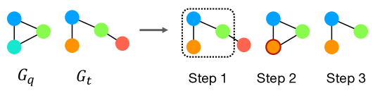
Figure 1: An example of computing SED between a query graph $G_{q}$ and a target graph $G_{t}$. The first step is to find an optimal subgraph in $G_{t}$. The last two steps are substituting a node label and deleting an edge in $G_{q}$, ending up SED as 2.

Subgraph Edit Distance (SED).  Given a query graph $G_{q}=(V_{q},E_{q},X_{q})$ and a target graph $G_{t}=(V_{t},E_{t},X_{t})$, SED represents the minimum cost of edits on $G_{q}$ such that the edited query is isomorphic to a subgraph in $G_{t}$. An edit operation can be inserting a node or an edge, deleting a node or an edge, or modifying a node or edge label (Zeng et al., 2009). Alternatively, the computation of SED seeks to identify a subgraph $G_{s}$ in the target graph $G_{t}$ such that $G_{s}$ and $G_{q}$ have the minimum graph edit distance (GED), which is the minimum number of edits that convert $G_{q}$ to be isomorphic $G^{\prime}_{t}$.

$$\mathrm{SED}(G_{t},G_{q})=\min_{G_{s}\subseteq G_{t}}\mathrm{GED}(G_{s},G_{q}).$$ (1)

Here we only consider connected graphs $G_{t}$ and $G_{q}$. Figure 1 illustrates an example of SED computation. In a geneal version of SED, each type of edit operation has a cost, which is application-dependent. Here we consider the basic version and set 1 as cost for all types of edits (e.g. (Zheng et al., 2013; Bai et al., 2019)).

Graph Neural Networks (GNNs).  GNNs learn node representations by iteratively updating node representations and sending messages to neighbors.

$$\mathbf{h}_{i}^{\prime}=\mathrm{UPDATE}\left(\mathbf{h}_{i},\mathrm{AGGREGATE}\left(\left\{\mathbf{h}_{j}:(i,j)\in E\right\}\right)\right).$$ (2)

Here $\mathrm{UPDATE}$ denotes an update function and $\mathrm{AGGREGATE}$ denotes an aggregation function. For example, $\mathrm{AGGREGATE}$ sums up all input vectors, and $\mathrm{UPDATE}$ is a dense layer that applies to the concatenation of its two arguments. $\mathbf{h}_{i}$ denotes the current representation of $i$, and $\mathbf{h}_{i}^{\prime}$ denotes updated representation. GNNs capture node features and topological features of a graph simultaneously (Wu et al., 2020b). GNN variants use different $\mathrm{UPDATE}$ and $\mathrm{AGGREGATE}$ functions. This work uses GATv2Conv (Brody et al., 2021), but other GNN alternatives such as Papp et al. (2021); Zhang & Li (2021) can also be considered. The choice of GNN architectures is a model selection problem , and we leave such exploration to the future.

A pooling function is often applied to aggregate all node vectors into a single graph vector.

$$\mathbf{z}=\mathrm{POOL}\left(\left\{\mathbf{h}_{i}:i\in V\right\}\right)$$ (3)

The $\mathrm{POOL}$ function is invariant to the order of elements in its input and has several implementations. For example, the $\mathrm{POOL}$ function can be an average function followed by a dense layer (Hamilton et al., 2017).

NeuroSED.  NeuroSED (Ranjan et al., 2021) is a neural network designed to mimic the calculation of SEDs from graph pairs. It uses Graph Isomorphism Network (GIN) (Xu et al., 2018) to encode both $G_{t}$ and $G_{q}$ into vectors and then predicts SED using a simple fixed function. Formally, NeuroSED writes as:

$$\mathbf{H}_{t}=\mathrm{GIN}(G_{t}),\quad\mathbf{H}_{q}=\mathrm{GIN}(G_{q}),$$ (4)

$$\mathrm{SED}=\left\lVert\mathrm{ReLU}\left(\mathrm{POOL}(\mathbf{H}_{q})-\mathrm{POOL}(\mathbf{H}_{t})\right)\right\rVert_{2}.$$ (5)

Here $\lVert\cdot\rVert_{2}$ is the $L_{2}$ norm.

4 Neural Graph Pruning for SED Calculation

4.1 Graph Pruning as a Node Relabeling Problem

Graph pruning aims to remove nodes in the target graph without affecting the SED between the target graph and the query graph. Suppose graph pruning keeps a node subset $V^{\prime}_{t}\subset V_{t}$ of the target graph and get the induced subgraph $G_{t}^{\prime}=(V^{\prime}_{t},E^{\prime}_{t},X_{t}(V^{\prime}_{t}))$. The purpose of pruning is to maintain that

$$SED(G_{t},G_{q})\approx SED(G^{\prime}_{t},G_{q})$$ (6)

while maximizing the number $|V_{t}|-|V^{\prime}_{t}|$ of pruned nodes. Graph pruning is a discrete operation, and the solution $V^{\prime}_{t}$ exists in a large searching space.

Here we formulate graph pruning as a node relabeling problem, which is more convenient for learning models.

We use a new node label $\phi\notin\Sigma$ to indicate that a node is pruned. Specifically, we relabel the target graph by $X^{\prime\prime}_{t}$ such that

$$X^{\prime\prime}_{t}(i)=\left\{\begin{array}[]{ll}X_{t}(i)&\mbox{if }i\in V^{\prime}_{t}\\ \phi&\mbox{otherwise}\end{array}\right.$$ (9)

Figure 2: Graph pruning in SED as a node relabeling problem. Gray nodes, which take the special label $\phi$, are treated as pruned.

We further assign a large cost (e.g. the size of $G_{t}$) to the edit operation that switches an actual label with $\phi$. Since the cost exceeds the edit distance from $G_{q}$ to any subgraph of $G_{t}$, the new graph $G_{t}^{\prime\prime}=(V_{t},E_{t},X^{\prime\prime}_{t})$ with relabeling is equivalent to the pruned graph $G^{\prime}$ in terms of SED calculation:

$$SED(G^{\prime}_{t},G_{q})=SED(G^{\prime\prime}_{t},G_{q}).$$ (10)

This is because the latter calculation will not match any node outside of $V^{\prime}_{t}$ to a node in $G_{q}$; otherwise, a node outside of $V^{\prime}_{t}$ will incur a large edit distance due to its new label $\phi$. A target graph with relabeling is shown in Figure 2.

To incorporate graph pruning in a neural network, we further formulate node relabeling to a continuous problem. In a neural network, the label of a node $i$ is usually expressed by a one-hot vector $\mathbf{x}_{i}=\mathrm{ONEHOT}(X_{t}(i))$, then we relabel each node $i$ by

$$\mathbf{x}^{\prime}_{i}=\alpha_{i}\mathbf{x}_{i}.$$ (11)

Here $\alpha_{i}$ is binary. If $\alpha_{i}=0$, which indicates the pruning of node $i$, then $\mathbf{x}^{\prime}_{i}$ is a zero vector, which is different from any one-hot representation of original labels in $\Sigma$. The vector $\mathbold{\alpha}=(\alpha_{i}:i\in V_{t})$ is a binary vector indicating which nodes are kept.

Then we relax the indicator vector to be continuous, $\mathbold{\alpha}\in[0,1]^{|V_{t}|}$. We call the continuous vector as keep probability: nodes with small probabilities are considered to be “pruned” from the graph. Now a neural network can compute $\mathbold{\alpha}$ from $G_{t}$ and $G_{q}$ as a learnable pruning component for neural SED calculation.

In the neural model, there is no need to specify the editing cost between a zero vector and a one-hot vector because the model can automatically decide it when fitting the training data. If $\mathbold{\alpha}$ reflexes accurate pruning, then a flexible learning model would avoid using nodes with zero vectors to predict accurate SED values.

4.2 Graph Pruning for SED Calculation

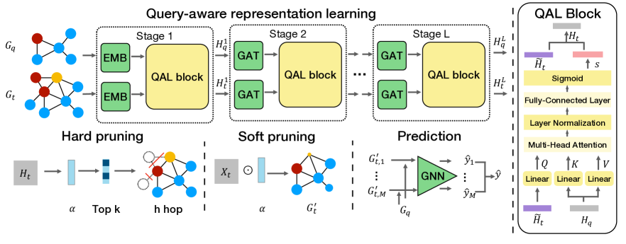
Figure 3: The overall framework of Prune4SED, including query-aware representation learning, hard/soft pruning, and multi-head SED prediction. The query-aware learning (QAL) block is implemented by a multi-head attention layer.

With the formulation above, we design an end-to-end neural model for computing SED. An overview of the model is depicted in Figure 3 (left). Specifically, Prune4SED  has three components, i.e., (1) query-aware representation learning, (2) hard/soft pruning, and (3) multi-head SED predicting. The first component learns node representation for $G_{t}$ conditioned on $G_{q}$. The second component learns to keep probability $\mathbold{\alpha}$ and also does the pruning. The third component predicts the final SED value.

Query-aware representation learning.  The representation learning component takes in the target $G_{t}$ and the query $G_{q}$ and outputs node representations of $G_{t}$. We design a neural architecture as the component to effectively use the information about $G_{q}$ when calculating node representations for $G_{t}$.

The core part of the component is the query-aware learning ($\mathrm{QAL}$) block, which allows the information of $G_{q}$ to flow into node representations of $G_{t}$. Figure 3 (right) shows the structure of $\mathrm{QAL}$. The inputs to the block are node representations $\mathbf{H}_{q}$ of $G_{q}$ and node representations $\widetilde{\mathbf{H}}_{t}$ of $G_{t}$. These representations are either from node features or learned by GNNs, which we will elaborate on later. Then the $\mathrm{QAL}$ block updates $\widetilde{\mathbf{H}}_{t}$ to new representations $\mathbf{H}_{t}$ using attention mechanism (Vaswani et al., 2017).

$$\mathbf{H}_{t}=\mathrm{QAL}\left(\widetilde{\mathbf{H}}_{t},\mathbf{H}_{q}\right).$$ (12)

The function of the $\mathrm{QAL}$ is specified as below:

$$\mathbf{H}_{t}=\mathrm{diag}(\mathbf{s})~{}\widetilde{\mathbf{H}}_{t},\quad\mathbf{s}=\mathrm{sigmoid}\left(\mathrm{MLP}(\mathbf{R})\right),\mathbf{R}=\mathrm{MHA}\left(\mathbf{Q}=\widetilde{\mathbf{H}}_{t},\mathbf{K}=\mathbf{V}=\mathbf{H}_{q}\right).$$ (13)

Here $\mathrm{MHA}$ is a multi-head attention layer (Vaswani et al., 2017) described in A.1. An intuitive understanding here is that representations of the target graph queries information from the query graph. Then we compute a weight vector $\mathbf{s}\in[0,1]^{|V_{t}|\times 1}$ that measures node importance in $G_{t}$. Then we scale $\widetilde{\mathbf{H}}_{t}$ according to $\mathbf{s}$, yielding the updated node representation $\mathbf{H}_{t}$ for $G_{t}$.

Now we are ready to compose the entire representation learning component with $\mathrm{QAL}$ blocks and GNN layers. We first use an embedding layer (the function $\mathrm{EMB}(\cdot)$) to encode node labels of both $G_{t}$ and $G_{q}$ into vector representations $\tilde{\mathbf{H}}^{1}_{t}$ and $\mathbf{H}_{q}^{1}$. Then we alternately apply $\mathrm{QAL}$ blocks and GNN layers to compute $G_{t}$ and $G_{q}$’s representations $\mathbf{H}_{t}^{l}$ and $\mathbf{H}_{q}^{l}$.

$$\mathbf{H}_{t}^{1}=\mathrm{QAL}\left(\widetilde{\mathbf{H}}_{t}^{1},\mathbf{H}_{q}^{1}\right),\quad\widetilde{\mathbf{H}}_{t}^{1}=\mathrm{EMB}\left(\mathbf{X}_{t}\right),\quad\mathbf{H}_{q}^{1}=\mathrm{EMB}\left(\mathbf{X}_{q}\right),$$ (14)

$$\mathbf{H}_{t}^{l}=\mathrm{QAL}\left(\widetilde{\mathbf{H}}_{t}^{l},\mathbf{H}_{q}^{l}\right),\quad\widetilde{\mathbf{H}}_{t}^{l}=\mathrm{GNN}\left(\mathbf{H}_{t}^{l-1},E_{t}\right),\quad\mathbf{H}_{q}^{l}=\mathrm{GNN}\left(\mathbf{H}_{q}^{l-1},E_{q}\right),\quad l=2,\ldots,L$$ (15)

Here $\mathrm{GNN}$ is a 1-layer graph attention convolution (Brody et al., 2021) (see A.2). The embedding layer and GAT layers are shared by $G_{q}$ and $G_{t}$.

We compute the final node representations $\mathbf{H}_{t}$ for $G_{t}$ using node representations after each $\mathrm{QAL}$ block.

$$\mathbf{H}_{t}=\mathrm{MLP}\left(\mathrm{CONCAT}\left(\mathbf{H}_{t}^{1}\ldots,\mathbf{H}_{t}^{L}\right)\right)$$ (16)

Here $\mathrm{CONCAT}$ concatenates node representations of $G_{t}$ at all stages to capture multi-granular views at various granularity levels. The MLP then encodes the concatenated node representations, further distilling essential information for pruning.

The query-aware learning component learns node representations of $G_{t}$ in the context of $G_{q}$. Each $\mathrm{QAL}$ block checks whether a node in $G_{t}$ can be matched to nodes in $G_{q}$ by considering their respective surrounding structures. Since GAT layers encode structural information at different levels of granularity, $\mathrm{QAL}$ blocks consider neighborhoods also at different levels. Therefore, it is beneficial to concatenate representations learned from all $\mathrm{QAL}$ blocks to capture information at different levels.

Hard/soft pruning.  Then we compute the keep probability $\mathbold{\alpha}$ for $G_{t}$ using $\mathbf{H}_{t}$.

We calculate $\mathbold{\alpha}$ from $G_{t}$’s node representations after each $\mathrm{QAL}$ block.

$$\mathbold{\alpha}=\mathrm{Sigmoid}\left(\frac{\mathbf{H}_{t}\mathbf{p}}{||\mathbf{p}||}\right).$$ (17)

Here $\mathbold{\alpha}$ is computed by a scalar projection along rows of $\mathbf{H}_{t}$ on a learnable vector $\mathbf{p}$, then it is scaled to $(0,1)$ by the $\mathrm{sigmoid}$ function. The projection is inspired by previous works in graph pooling (Gao & Ji, 2019; Cangea et al., 2018; Knyazev et al., 2019).

Next we use $\mathbold{\alpha}$ to prune $G_{t}$. Before we apply the type of pruning we discussed in equation 11, we first apply hard pruning to remove some nodes from $G_{t}$. We first keep a set $S$ of $k$ nodes corresponding to the largest value in $\mathbold{\alpha}$. We also keep all $h$ hop neighbors of each node in $S$ to increase connectivity and balance computation and information loss. Then we get a set $V^{\prime}_{t}$ of nodes as the result of hard pruning from $\mathbold{\alpha}$. Thus, we define hard pruning as follows:

$$S=\mathrm{top\_}k(\mathbold{\alpha}),$$ (18)

$$V_{t}^{\prime}=h\mbox{\_}\mathrm{hop}(S,G_{t}),$$ (19)

Here $\mathrm{top\_}k(\mathbold{\alpha})$ selects top $k$ nodes corresponding to the $k$ largest values in $\mathbold{\alpha}$; and $h\mbox{\_}\mathrm{hop}(S,G_{t})$ extracts $h$ hop neighbors surrounding nodes in $S$.

The hard pruning is useful when $G_{t}$ has a much larger diameter than $G_{q}$. In this case, it removes a decent fraction of nodes in $G_{t}$, which is beneficial to both accuracy and speed. Later we show the effectiveness of hard pruning in real examples in Figure 5, . Hard pruning shares the same principle as Graph U-Net (Gao & Ji, 2019), which shows that the discrete operation does not pose issues to loss minimization.

Then we apply $\mathbold{\alpha}$ to these nodes in $V^{\prime}_{t}$ to do soft pruning as introduced in Section 4.1.

$$X^{\prime}_{t}(i)=\alpha_{i}X_{t}(i),\quad i\in V_{t}^{\prime}$$ (20)

The pruned graph is $G^{\prime}_{t}=(V^{\prime}_{t},E^{\prime}_{t},X^{\prime}_{t})$. Here $E^{\prime}_{t}$ keeps all $G_{t}$’s edges that are incident with nodes in $V^{\prime}_{t}$.

We put the entire pruning procedure into a single function $G^{\prime}_{t}=\mathrm{PRUNE}(\mathbf{H}_{t},G_{t})$, which computes $\mathbold{\alpha}$ from $\mathbf{H}_{t}$ and then executes hard and soft pruning on $G_{t}$ to get $G^{\prime}_{t}$. Note that soft pruning is differentiable and helps to learn the keep probability $\alpha$. The model learns to use small keep probabilities to indicate that their corresponding nodes cannot be matched to nodes in the query graph. Hard pruning is not differentiable, but it is still meaningful to remove nodes with small keep probabilities.

Multi-head prediction of SEDs.  Once we have the pruned graph $G^{\prime}_{t}$, we use a neural module to “predict” the SED between $G^{\prime}_{t}$ and $G_{q}$. For example, we can use the NeuralSED network as the predictive module.

However, given the combinatorial nature of graph pruning, there might be many locally optimal solutions of $\mathbold{\alpha}$, and it is hard for the model to identify good $\mathbold{\alpha}$ values in one-shot. Inspired by multi-head attention, we propose a multi-head predicting module.

We use $M$ separate pruning functions, ($\mathrm{PRUNE}_{1},\ldots,\mathrm{PRUNE}_{M}$), each of which optimizes its own parameter $\mathbf{p}_{m}$ in equation 17, to obtain $M$ different pruned graphs $G^{\prime}_{t,1},\ldots,G^{\prime}_{t,M}$. Then we use the same predictive module $\mathrm{PRED}$ to compute SED values from these pruned graphs.

$$G^{\prime}_{t,m}=\mathrm{PRUNE}_{m}\left(\mathbf{H}_{t},G_{t}\right),\quad\hat{y}_{m}=\mathrm{PRED}(G^{\prime}_{t,m},G_{q}),\quad m=1,\ldots,M.$$ (21)

Then we take the average to get the final prediction.

$$\hat{y}=\mathrm{MEAN}\left(\hat{y}_{1},\ldots,\hat{y}_{M}\right).$$ (22)

Here we use NeuroSED in equation 5 as the $\mathrm{PRED}$ function.

With multi-head pruning our model is able to explore multiple ways of pruning $G_{t}$ and thus has chances to capture good ones. At the same time, we only compute multiple prunings from different projections of the same set of node representations, so we only slightly increase the number of parameters.

Algorithm 1 Prune4SED

1:Input: $G_{q},G_{t}$

2:$\triangleright$ Query-aware representation learning

3:for $l$ = 1 to $L$ do

4:     $\widetilde{\mathbf{H}}_{t}^{l},\mathbf{H}_{q}^{l}=\begin{cases}\mathrm{EMB}\left(\mathbf{X}_{t}\right),~{}\mathrm{EMB}\left(\mathbf{X}_{q}\right),&\text{if $l=1$}\\ \mathrm{GAT}\left(\mathbf{H}_{t}^{l-1},E_{t}\right),~{}\mathrm{GAT}\left(\mathbf{H}_{q}^{l-1},E_{q}\right),&\text{o.w.}\end{cases}$

5:     $\mathbf{H}_{t}^{l}=\mathrm{QAL}(\widetilde{\mathbf{H}}_{t}^{l},\mathbf{H}_{q}^{l})$ $\triangleright$ QAL block from equation 12

6:end for

7:$\mathbf{H}_{t}=\mathrm{MLP}\left(\mathrm{CONCAT}\left(\mathbf{H}_{t}^{1}\ldots,\mathbf{H}_{t}^{L}\right)\right)$

8:for $m$ = 1 to $M$ do $\triangleright$ Multi-head pruning

9:     $G^{\prime}_{t,m}=\mathrm{PRUNE}_{m}\left(\mathbf{H}_{t},G_{t}\right)$

10:     $\hat{y}_{m}=\mathrm{PRED}(G^{\prime}_{t,m},G_{q})$

11:end for

12:$\hat{y}=\mathrm{MEAN}\left(\hat{y}_{1},\ldots,\hat{y}_{M}\right)$

13:Return $\hat{y}$

4.3 Optimization

Prune4SED  is summarized in Algorithm 1. First, query-aware representation learning encodes target graph $G_{t}$ (Line 1-5). Then multi-head pruning is used to prune $G_{t}$ from multiple views to predict SED (Line 6-9). Each head contains a sequence of operations, including $\mathbold{\alpha}$ computation, hard/soft pruning, and SED prediction. Finally, predictions from multi-head pruning are combined as the final prediction (Line 10).

For model training, model predictions are compared against SED values computed by a MIP-F2 solver (Lerouge et al., 2017). Given a pair of graphs $(G_{t},G_{q})$, the model makes a prediction $\hat{y}$. For the same pair the solver returns a lower bound $y_{L}$ and an upper bound $y_{U}$ of the true solution. In most cases $y_{L}=y_{U}$, which means that the solver find the true solution. For the same pair. To handle the general case, we penalize the prediction with a squared error when it is outside of $[y_{L},y_{U}]$. We minimize the following training loss computed from a dataset $\mathcal{D}$ to train the model.

$$\min~{}~{}\mathcal{L}=\sum_{(G_{q},G_{t})\in\mathcal{D}}([y_{L}-\hat{y}]_{+})^{2}+([\hat{y}-y_{U}]_{+})^{2}$$ (23)

Here $[\cdot]_{+}$ truncate negative values to zero. The loss is equivalent to squared loss when $y_{L}=y_{U}$.

Next we analyze time complexity of Prune4SED. We first consider graph sizes. The attention layer in the $\mathrm{QAL}$ block needs to consider every node in $G_{t}$ against every node in $G_{q}$, so its running time is $O(|V_{t}|\cdot|V_{q}|)$. GAT layers runs in linear time about $O(|E_{t}|+|E_{q}|)$. Processing node vectors need time $O(|V_{t}|+|V_{q}|)$, so the overall running time is $O(|E_{t}|+|E_{q}|+|V_{t}|\cdot|V_{q}|)$.

The running time is in linear time with network hyperparameters, including the width of the network, the number of layers, the number of attention heads, or the number of pruning heads.

5 Experiments

In this section, we aim to validate the effectiveness of Prune4SED through experiments and also examine the model to understand how it works. We have the following sub-aims: 1) benchmarking the performance of Prune4SED  against existing SED solvers/predicting models; 2) understanding the usefulness of our model designs through ablation studies; 3) examining pruned graphs to check whether neural graph pruning aligns with SED calculation; and 4) applying the model to a real-world applications.

Experiment settings.  By default, we use $L=5$ stages for Prune4SED. In hard pruning, we take top $k$ $(k=5)$ important nodes and their $h$ $(h=L-1=4)$ hop neighbors. The SED predictor contains an 8-layer GIN with 64 hidden units at every layer. We use $M=5$ heads to produce the final prediction. More details about model hyperparameters and platforms are given in B.2.

Datasets.  We use seven datasets (AIDS, CiteSeer, Cora_ML, Amazon, DBLP, PubMed, and Protein) to evaluate our model for SED approximation. B.1 provides more descriptions about these datasets.

Table 1: Dataset Statistics.

Dataset	$|V_{q}|$	$|V_{t}|$	$|\Sigma|$
AIDS	9	14	38
CiteSeer	12	73	6
Cora_ML	11	98	7
Amazon	12	43	1
DBLP	14	240	8
PubMed	12	60	3
Protein	9	38	3

We extract query-target pairs from each dataset to train, validate, and test models. For datasets with a single network (CiteSeer, Cora_ML, Amazon, DBLP, and PubMed), the target graph $G_{t}$ is a ego-net (up to 5-hop) of a random node sampled from large network. For datasets with multiple graphs (AIDS and Protein), the target graph is a graph in the dataset. Except the AIDS datset, the query graph is a subgraph from a random target graph (sampled from all target graphs). The subgraph is randomly sampled by starting from the center node of the target $G_{t}$, progressively selecting unseen neighbors with a probability 0.5 of the current nodes, and stopping at a depth up to 5. Query graphs of the AIDS dataset are known functional groups from Ranu & Singh (2009). To compute the SED between $G_{q}$ and $G_{t}$, we use a mixed-integer-programming solver, MIP-F2 (Lerouge et al., 2017). The solver runs on a 64 core machine with maximum of 60 seconds to compute lower and upper bounds the true SED. From each dataset, we randomly pair target and query graphs to get 100K pairs for training, 10K for validation, and another 10K for testing. Table 1 shows average sizes (rounded to 1) of target and query graphs and the number of node labels in the data extracted from each dataset.

Baselines.  We compare Prune4SED with five other approaches. The first three are neural models: H²MN (Zhang et al., 2021), SIMGNN (Bai et al., 2019), and NeuroSED (Ranjan et al., 2021). For H²MN and SIMGNN, we use their modified versions from Ranjan et al. (2021) that better suit SED prediction. For H²MN, we include its two versions of random walks (H²MN-RW) and the k-hop version (H²MN-NE). The second comparison contains two non-neural methods MIP-F2 (Lee et al., 2010a) and BRANCH (Blumenthal, 2019), both of which are implemented by an efficient C++ library GEDLIB (Blumenthal et al., 2019; 2020). As competing methods, both are given 0.1 second to compute the upper bound $y_{U}$ and lower bounds $y_{L}$ of the true SED, then $\hat{y}=(y_{U}+y_{L})/2$ is used as the prediction. Note that 0.1 second is already much longer than our model’s predicting time.

The predictive performance of these models is evaluated by root-mean-square error (RMSE), which is the square root of the mean squared error defined in equation 23.

Table 2: RMSE on seven datasets.

	AIDS	CiteSeer	Cora_ML	Amazon	Dblp	PubMed	Protein
Branch	1.379	3.161	3.102	4.513	2.917	2.613	2.391
MIP-F2	1.537	4.474	3.871	5.595	3.427	3.399	2.249
H2MN-RW	0.749	1.502	1.446	1.294	1.47	1.213	0.941
H2MN-NE	0.657	1.827	1.229	0.971	1.552	1.326	0.755
SIMGNN	0.696	1.781	1.289	2.81	1.482	1.322	1.223
NeuroSED	0.512	0.519	0.635	0.495	0.964	0.728	0.524
Prune4SED	0.480	0.365	0.437	0.322	0.859	0.447	0.485
Improv. over best baseline	6.3%	29.7%	31.2%	34.9%	10.9%	38.6%	7.4%
Prune4SED  w/o. $\mathrm{QAL}$	0.496	0.439	0.575	0.359	0.953	0.585	0.505
Prune4SED  w. 1 head	0.497	0.383	0.458	0.324	0.915	0.469	0.495
Prune4SED  w. 10 heads	0.482	0.373	0.449	0.321	0.817	0.488	0.488

5.1 Benchmark Predictive Performances

Table 2 summarizes performances of different models. The results of baselines are taken from Ranjan et al. (2021). The results show that neural methods outperform non-neural methods (Branch and MIP-F2). This is consistent with findings in previous work. H2MN and SIMGNN are designed for Graph Edit Distance. They compare the entire target graph to the query to compute the target value. This calculation is not appropriate for SED because many nodes in the target graph are irrelevant to the true SED.

Prune4SED outperforms all baselines and establishes new state-of-the-art performances across all seven datasets in terms of RMSE, as shown in Table 2. Specifically, Prune4SED substantially improves the best neural solver, NeuroSED, with an average of 23% improvement. Our analysis later shows that our model gains an advantage by removing some irrelevant nodes from the target graph before predicting SED values.

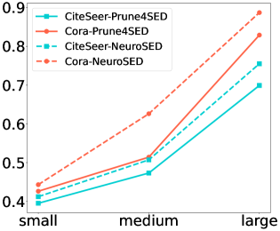
Figure 4: RMSE versus node number

We further study the performance of our model with graph sizes. By controlling the random sampling procedure, we get graph pairs with different sizes and form three sets (small, medium, and large) of graph pairs. Each set has 2000 query-target pairs. We separately extract such sets from Cora_ML and Citeseer datasets. In the three sets (small/medium/large), the target graphs extracted from CiteSeer have average sizes 16/62/122, and those extracted from Cora have average sizes 17/64/118. The average sizes of queries are about 12 across all sets extracted from the two datasets. Each set are split into training (80%) , validation (10%), and testing (10%). We run our model on each set to get an RMSE, then we can plot RMSEs from three sets against their sizes. We also run NeuroSED as a baseline here for a comparison.

Table 3: Inference time (seconds).

Dataset	Cora_ML	CiteSeer
MIP-F2	$1.0\times 10^{-1}$	$1.0\times 10^{-1}$
NeuroSED	$1.5\times 10^{-4}$	$1.5\times 10^{-4}$
Prune4SED	$1.9\times 10^{-3}$	$1.7\times 10^{-3}$

Figure 4 shows the results. We see that both models have worse performances on larger graphs, which indicates that SED problems on larger graphs are more challenging for neural models. Nevertheless, the RMSE of our model is less than 1, which is still fairly accurate, considering that query graphs often have dozens of edges. Our model is still significantly better than NeuroSED.

We also test the predicting time of all models and report the comparison in Table 3. The optimization-based approach for SED calculation can take very long time to get the true answer. Here we give a time limit of 0.1 second to MIP-F2, and the time is already much longer than the prediction time of neural methods, but its performance is worse than neural methods as we have shown above. Prune4SED is slower than NeuroSED because it uses more neural layers. But considering the performance improvement, our model still has advantages in many applications. Furthermore, the computation time is not relevant to graph sizes and thus can be sped up by improving network architectures. We leave such work to the future.

5.2 Examine pruned graphs

To understand the good performance of the proposed model, we examine how the model prunes target graphs. We visualize a few examples of hard and soft pruning over the graph in Figure 5. Here node colors represent node labels. Nodes removed by hard pruning are not shown in the figure, and node sizes are proportional to keep probabilities.

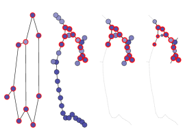
(a) $\quad\quad~{}G_{q}\quad\quad~{}G_{t}\quad\quad~{}\text{hard}\quad\quad\quad\text{soft}$

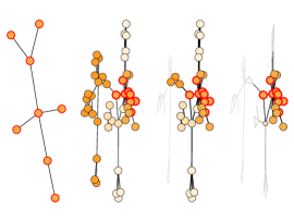
(b) $\quad\quad G_{q}\quad\quad~{}G_{t}\quad\quad~{}\text{hard}\quad\quad~{}~{}\text{soft}$

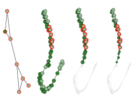
(c) $\quad~{}~{}G_{q}\quad\quad~{}G_{t}\quad\quad\text{hard}\quad\quad\text{soft}$

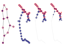
(d) AIDS

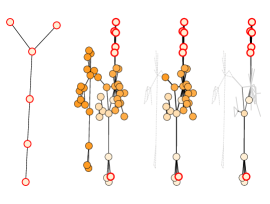
(e) CiteSeer

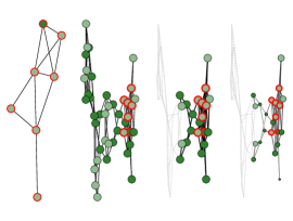
(f) Protein

Figure 5: Visualization of pruned graphs on AIDS, CiteSeer, and Proteins datasets. Every four graphs is a group, representing query graph $G_{q}$, target graph $G_{t}$, target graph after hard pruning and after soft pruning. Node colors represent node labels. In soft pruning, nodes are resized according to their keep probabilities. Nodes with red circles mark the optimal subgraph.

These examples show that the pruning component removes a significant amount of unrelated nodes in the target graph. Hard and soft prunings obtained from $\mathbold{\alpha}$ are reasonable for matching the query. In the first example, it removes the long-chain, which obviously cannot match the query graph. We also observe that the pruning of the same target graph is different for different query graphs. In the AIDS example, nodes at the top part of the target graph are pruned differently; In the CiteSeer example, the nodes on the right side are pruned differently. It is a strong indication that the model does consider the query graph when it prunes the target graph.

We further check the effect of graph pruning over SED calculations. Ideally graph pruning should not affect SED calculation, that is, SEDs computed from pruned graphs should still be the same as SEDs computed from original target graphs. We truncate keep probabilities with a threshold and then prune all nodes with probabilities below the threshold, then we run an exact SED solver to check how much this hard way of pruning affects the SED. If the SED does not change much, then it means that node probabilities do indicate a good pruning of the target graph.

We conduct this experiment with 500 randomly selected graphs from the AIDS, CiteSeer, and Protein datasets. We adjust the threshold to prune $r=0.1$, $0.3$, and $0.5$ of all graph nodes. Then we compare the calculated SEDs against SEDs computed from the original graphs (ground truth). The solver cannot get the true SED for a small number of cases, then we use $(y_{U}+y_{L})/2$ as the true SED. We use MAE to measure the difference and also compute the correlation coefficient between the two groups of SEDs.

Table 4 summarizes the results of MAE and correlation coefficient. We see that the difference is fairly small when the ratio is small. When the pruning ratio is low (0.1 and 0.3), SEDs computed from pruned graphs only have slight differences with SEDs computed from the original graph. The average difference is less than 0.04 on the first two datasets and only 0.11 on the third dataset; the Pearson correlation coefficient is above 0.99. When the pruning ratio is as aggressive as 0.5, the difference is still at an acceptable level. Figure 6 further visualizes the correlation between SEDs computed from original graphs and pruned graphs respectively. The size of dots in the figure indicate the number of graph pairs occurring at that location in the plot. We again see that pruning does not affect SED computation on most graphs. These results confirm that our pruning weights correctly recognize and retain important nodes in $G_{t}$.

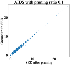
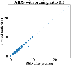
Figure 6: Correlation between SEDs computed from pruned graphs and SEDs computed from the original graphs. The size of dots indicates the number of SED pairs occurring at that location.

Table 4: Pearson correlation coefficient $\rho$ and mean absolute error (MAE) computed between ground truth SED and SED computed from pruned graph using an exact solver. The pruning ratio $r$ indicates the average node ratio impacted by hard pruning and soft pruning per graph. Larger results are better for $\rho$ and smaller results are better for MAE.

Dataset	$r=0.1$		$r=0.3$		$r=0.5$
	$\rho$ $\uparrow$	MAE $\downarrow$	$\rho$ $\uparrow$	MAE $\downarrow$	$\rho$ $\uparrow$	MAE $\downarrow$
AIDS	0.999	0.026	0.998	0.036	0.983	0.144
CiteSeer	1.000	0.022	1.000	0.026	1.000	0.032
Protein	0.996	0.092	0.995	0.110	0.980	0.237

5.3 Ablation Studies

We conduct two ablation studies to investigate the effectiveness of the QAL block and multi-head pruning, and we report results in the bottom three rows 2.

Query-aware representation learning.  Recall that query-aware learning aims to leverage query graph to learn representations for the target graph so that neural graph pruning is adaptive to the query graph.

To this end, we compare Prune4SED with and without query-aware learning. In the setup of Prune4SED without query-aware learning, we remove all $\mathrm{QAL}$ blocks in representation learning (i.e., $\mathbf{H}_{t}^{l}=\tilde{\mathbf{H}}_{t}^{l}$ in equation 14 and equation 15 ). Therefore, representation learning solely depends on the target graph.

We see that removing $\mathrm{QAL}$ blocks consistently increases RMSE values across seven datasets. The results verify the effectiveness of query-aware learning in terms of extracting information from query graphs.

(a) $G_{q}$

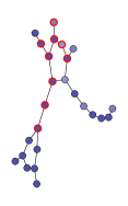
(b) $G_{t}$

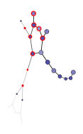
(c) Head 1

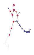
(d) Head 2

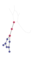
(e) Head 3

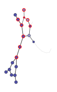
(f) Head 4

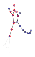
(g) Head 5

Figure 7: Multiple heads have learned different pruning strategies. By average, the final prediction obtained from multiple heads is close to ground truth (4.1 v.s. 4).

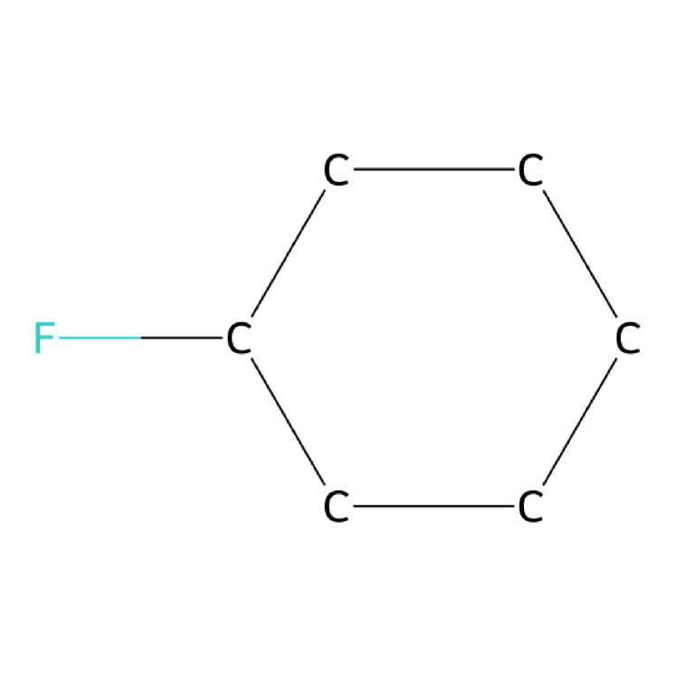
(a) Query

(b) SED/Prune4SED

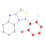
(c) 0/0.4

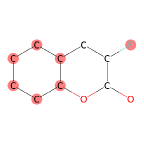
(d) 1/0.4

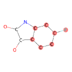
(e) 0/0.5

(f) 0/0.5

(g) 0/0.5

(h) SED/NeuroSED

(i) 0/0.6

(j) 1/0.6

(k) 1/0.6

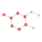
(l) 1/0.6

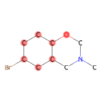
(m) 1/0.7

Figure 8: Retrieving chemical compounds given a query graph, which is a functional group. The retrieved compounds are ranked according to their predicted SED. Two values under each compound are ground truth SED and predicted SED.

Multi-head pruning.  We use $M=1$, $M=5$ (default), and $M=10$ heads to Prune4SED and compare their performances. Prune4SED with multiple heads ($M=5$ and $M=10$) clearly improves the performance compared with Prune4SED with a single predictive head, confirming the contribution of multiple heads. The results also suggest that $M=5$ is a reasonable choice in practice.

Figure 7 further show an example where five predictive heads prune the target $G_{t}$ in different ways. Multiple predictive heads allow the model to discover more structures that are similar to the query graph and smooth out some predictive errors. The final prediction (averaged over 5 heads) is close to the ground truth (ground truth SED is 4, and the predicted SED is 4.1).

5.4 Application: Molecular Fragment Containment Search

Molecular fragment containment searching is a fundamental problem in drug discovery (Ranu et al., 2011; Ranjan et al., 2021). The problem can be formulated as a standard problem of subgraph similarity search: given a query graph representing some functional group, the task is to retrieve from a database chemical compounds that contain the functional group.

We apply Prune4SED to solve this task. We evaluate on AIDS dataset, where target graphs are antivirus screen chemical compounds collected from NCI and query graphs are known functional groups. The dataset does not include Hydrogen atoms.

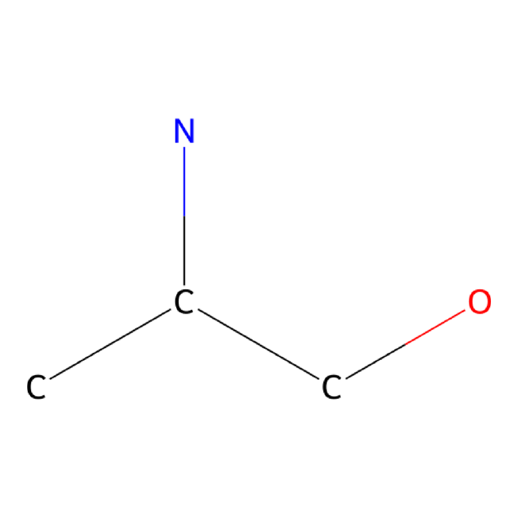
(a) Query

(b) SED/Prune4SED

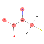
(c) 0/0.0

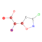
(d) 0/0.1

(e) 0/0.1

(f) 0/0.1

(g) 0/0.1

(h) SED/NeuroSED

(i) 0/0.2

(j) 1/0.2

(k) 1/0.2

(l) 0/0.2

(m) 0/0.2

(n) Query

(o) SED/Prune4SED

(p) 0/0.8

(q) 1/0.9

(r) 1/1.0

(s) 1/1.1

(t) 1/1.1

(u) SED/NeuroSED

(v) 0/1.2

(w) 2/1.3

(x) 2/1.4

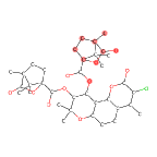
(y) 2/1.4

(z) 3/1.5

Figure 12: Retrieving chemical compounds given a query graph, which is a functional group.

Figure 8 visualizes one set of retrieval results. The five molecules with the smallest predicted SEDs are shown in the Figure. Four out of these five molecules actually contain the function group. Prune4SED has better retrieval results than NeuroSED. More examples can be found in Figure 12 of B.4.

We also observe that Prune4SED can find molecules that contain the query but is much larger than the query. We hypothesize that our model is able to prune unnecessary nodes and identify the subgraph corresponding to the query, while NeuroSED either tries to find target graphs that are similar to the query graph or bet its luck on very large molecules. It is another evidence that pruning is necessary for SED calculation.

6 Conclusion

In this work, we study the problem of using a learning model to predict the SED between a target graph and a query graph. We present Prune4SED, an end-to-end model to address the problem. Notably, Prune4SED learns to prune the target graph to reduce interference from irrelevant nodes. It converts graph pruning to a node relabeling problem and enables pruning in a differentiable neural model. Our new model Prune4SED combines two novel techniques, query-aware representation learning and multi-head pruning to improve the model’s ability of learning good prunings. Extensive experiments validate the superiority of Prune4SED.

Acknowledgments

We thank all reviewers and editors for their insightful comments. Linfeng Liu and Li-Ping Liu were supported by NSF 1908617. Xu Han was supported by Tufts RA support. Part of the computation resource is provided by Amazon AWS.

Appendix A Additional preliminaries

A.1 Multi-Head Attention

Transformer (Vaswani et al., 2017) has been proved successful in the NLP field. The design of multi-head attention (MHA) layer is based on attention mechanism with Query-Key-Value (QKV). Given the packed matrix representations of queries $\mathbf{Q}$, keys $\mathbf{K}$, and values $\mathbf{V}$, the scaled dot-product attention used by Transformer is given by:

$$\mathrm{ATTENTION}(\mathbf{Q},\mathbf{K},\mathbf{V})=\mathrm{softmax}\left(\frac{\mathbf{Q}\mathbf{K}^{T}}{\sqrt{D_{k}}}\right)\mathbf{V},$$ (24)

where $D_{k}$ represents the dimensions of queries and keys.

The multi-head attention applies $H$ heads of attention, allowing a model to attend to different types of information.

$$\mathrm{MHA}(\mathbf{Q},\mathbf{K},\mathbf{V})=\mathrm{CONCAT}\left(\mathrm{head}_{1},\ldots,\mathrm{head}_{H}\right)\mathbf{W}$$

$$\mathrm{where}\quad\mathrm{head}_{i}=\mathrm{ATTENTION}\left(\mathbf{Q}\mathbf{W}_{i}^{Q},\mathbf{K}\mathbf{W}_{i}^{K},\mathbf{V}\mathbf{W}_{i}^{V}\right),i=1,\ldots,H.$$ (25)

A.2 GATv2 Convolution

We use GATv2 (Brody et al., 2021) as $\mathrm{GAT}$ in equation 15. GATv2 improves GAT (Veličković et al., 2017) through dynamic attention, fixing the issue of GAT that the ranking of attention scores is unconditioned on query nodes. In GATv2, each edges $(j,i)\in E$ has a score to measure the importance of node $j$ to node $i$. The score is computed as

$$e\left(\mathbf{h}_{i},\mathbf{h}_{j}\right)=\mathbf{a}^{\mathrm{T}}\mathrm{LeakyReLU}\left(\mathbf{W}\left[\mathbf{h}_{i}~{}||~{}\mathbf{h}_{j}\right]\right),$$ (26)

where $\mathbf{a}$ and $\mathbf{W}$ are learnable parameters, and $||$ concatenates two vectors. These score are compared across the neighbor set of $i$, obtaining normalized attention scores,

$$\theta_{i,j}=\frac{\exp\left(e\left(\mathbf{h}_{i},\mathbf{h}_{j}\right)\right)}{\exp\left(\sum_{j^{\prime}\in\mathcal{N}(i)}e\left(\mathbf{h}_{i},\mathbf{h}_{j^{\prime}}\right)\right)}.$$ (27)

The representation of $i$ is then updated using an nonlinearity $\gamma$,

$$\mathbf{h}^{\prime}_{i}=\gamma\left(\sum_{j\in\mathcal{N}(i)}\theta_{i,j}\cdot\mathbf{W}\mathbf{h}_{j}\right).$$ (28)

Appendix B Experiment details

B.1 Dataset

AIDS.  AIDS dataset contains a collection of antiviral screen chemical compounds published by National Cancer Institute (NCI). Each graph represents a chemical compound with nodes as atoms and edges as chemical bonds. Hydrogen atoms are omitted. Notably, the queries of AIDS dataset are known functional groups from Ranu & Singh (2009).

Citation networks.  Cora_ML, CiteSeer, and PubMed are citation networks (Sen et al., 2008; Bojchevski & Günnemann, 2017). In each dataset, nodes represent publications and edges correspond to citation relations. Each node in the datasets has a feature vector derived from words in the publication.

Amazon.  Amazon dataset (Leskovec & Sosič, 2016) contains a collection of products as nodes. Two nodes are connected if they are frequently co-purchased.

DBLP.  DBLP is a co-author network (Tang et al., 2008). Each node represents an author. Edges link any two authors that appeared in a paper.

Protein.  Protein dataset contains graphs describing proteins (Dobson & Doig, 2003; Fey & Lenssen, 2019). Nodes represent secondary structure elements. Edges link two nodes if they are neighbors along the amino acid sequence or they are near in space.

B.2 Model hyperparameters

We use stochastic optimizer AdamW (Loshchilov & Hutter, 2017) with batch size 200. We set learning rate using a cyclical learning rate policy (CLR) (Smith, 2017), with each round learning rate increasing from 0 to $10^{-3}$ in 2000 iterations then decreasing back to 0 in another 2000 iterations. Weight decay is set to be $10^{-3}$. Validation set is used to early stop training if no improvement is observed in 5 rounds. We conduct experiments on a cluster of NVIDIA A100 GPUs.

Our predictor design follows NeuroSED (Ranjan et al., 2021) as written in equation 5. We also test NeuroSED using a $\mathrm{MLP}$ as the final layer to predict SED, $\mathrm{SED}=\mathrm{MLP}\left([\mathrm{POOL}(\mathbf{H}_{t})~{}\|~{}\mathrm{POOL}(\mathbf{H}_{q})]\right)$. We found the practical performance between the two versions is neglectable (relative difference on RMSE is around 1%).

B.3 Parameter sensitivity.

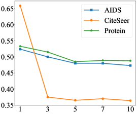
(a) $\mathrm{top}\_k$

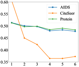
(b) $h\mbox{\_}\mathrm{hop}$

Figure 9: Sensitivity analysis of the two pruning hyper-parameters ($\mathrm{top}\_k$ and $h\mbox{\_}\mathrm{hop}$). Left: RMSEs by varying $k$ in $\mathrm{top}\_k$ with 4 hops ($h$ = 4). Right: RMSEs by varying $h$ in $h\mbox{\_}\mathrm{hop}$ ($k=5$).

We evaluate two important hyperparamters in Prune4SED, $k$ in $\mathrm{top\_}k$ and $h$ in $h\mbox{\_}\mathrm{hop}$. Smaller $k$ and $h$ lead to more aggressive pruning. We examine how Prune4SED performs at different values of $k$ and $h$. We see in Figure 9, Prune4SED performs well across multiple datasets when $k$ and $h$ are sufficiently large (e.g. $k=5$ and $h=5$). When $k$ and $h$ are large enough, soft pruning will play the main role and still maintain a good performance. It indicates that the two hyper-parameters are relatively easy to tune so the model adapts to different datasets.

B.4 More results

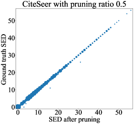
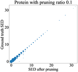
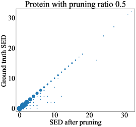
Figure 10: Correlation between SEDs computed from pruned graphs and SEDs computed from the original graphs.

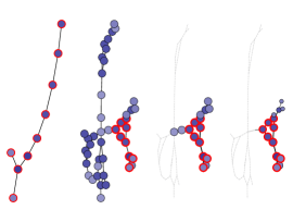
(a) $\quad~{}~{}G_{q}\quad\quad G_{t}\quad\quad\quad\text{hard}\quad\quad~{}\text{soft}$

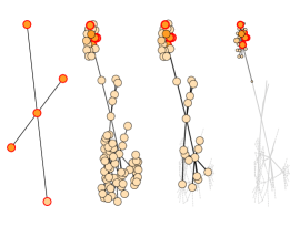
(b) $\quad~{}G_{q}\quad\quad~{}G_{t}\quad\quad~{}\text{hard}\quad\quad~{}~{}\text{soft}$

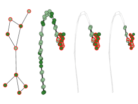
(c) $\quad~{}~{}G_{q}\quad\quad G_{t}\quad\quad~{}\text{hard}\quad\quad~{}~{}\text{soft}$

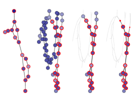
(d) AIDS

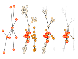
(e) CiteSeer

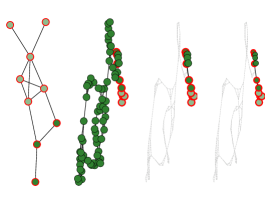
(f) Protein

Figure 11: Visualization of pruned graphs on AIDS, CiteSeer, and Proteins.

References

- Bai et al. (2019) Yunsheng Bai, Hao Ding, Song Bian, Ting Chen, Yizhou Sun, and Wei Wang. Simgnn: A neural network approach to fast graph similarity computation. In Proceedings of the Twelfth ACM International Conference on Web Search and Data Mining, pp. 384–392, 2019.
- Bai et al. (2020) Yunsheng Bai, Hao Ding, Ken Gu, Yizhou Sun, and Wei Wang. Learning-based efficient graph similarity computation via multi-scale convolutional set matching. In Proceedings of the AAAI Conference on Artificial Intelligence, volume 34, pp. 3219–3226, 2020.
- Blumenthal (2019) David B Blumenthal. New techniques for graph edit distance computation. arXiv preprint arXiv:1908.00265, 2019.
- Blumenthal et al. (2019) David B Blumenthal, Sébastien Bougleux, Johann Gamper, and Luc Brun. Gedlib: a c++ library for graph edit distance computation. In International Workshop on Graph-Based Representations in Pattern Recognition, pp. 14–24. Springer, 2019.
- Blumenthal et al. (2020) David B Blumenthal, Nicolas Boria, Johann Gamper, Sébastien Bougleux, and Luc Brun. Comparing heuristics for graph edit distance computation. The VLDB Journal, 29(1):419–458, 2020.
- Bojchevski & Günnemann (2017) Aleksandar Bojchevski and Stephan Günnemann. Deep gaussian embedding of graphs: Unsupervised inductive learning via ranking. arXiv preprint arXiv:1707.03815, 2017.
- Bougleux et al. (2017) Sebastien Bougleux, Luc Brun, Vincenzo Carletti, Pasquale Foggia, Benoit Gaüzère, and Mario Vento. Graph edit distance as a quadratic assignment problem. Pattern Recognition Letters, 87:38–46, 2017.
- Brody et al. (2021) Shaked Brody, Uri Alon, and Eran Yahav. How attentive are graph attention networks? arXiv preprint arXiv:2105.14491, 2021.
- Bunke (1997) Horst Bunke. On a relation between graph edit distance and maximum common subgraph. Pattern Recognition Letters, 18(8):689–694, 1997.
- Cangea et al. (2018) Cătălina Cangea, Petar Veličković, Nikola Jovanović, Thomas Kipf, and Pietro Liò. Towards sparse hierarchical graph classifiers. arXiv preprint arXiv:1811.01287, 2018.
- Cappart et al. (2021) Quentin Cappart, Didier Chételat, Elias B. Khalil, Andrea Lodi, Christopher Morris, and Petar Veličković. Combinatorial optimization and reasoning with graph neural networks. In Proceedings of the Thirtieth International Joint Conference on Artificial Intelligence, IJCAI-21, pp. 4348–4355. International Joint Conferences on Artificial Intelligence Organization, 2021.
- Chen et al. (2020) Zhengdao Chen, Lei Chen, Soledad Villar, and Joan Bruna. Can graph neural networks count substructures? Advances in neural information processing systems, 33:10383–10395, 2020.
- Daller et al. (2018) Évariste Daller, Sébastien Bougleux, Benoit Gaüzère, and Luc Brun. Approximate graph edit distance by several local searches in parallel. In 7th International Conference on Pattern Recognition Applications and Methods, 2018.
- Dobson & Doig (2003) Paul D Dobson and Andrew J Doig. Distinguishing enzyme structures from non-enzymes without alignments. Journal of molecular biology, 330(4):771–783, 2003.
- Fankhauser et al. (2011) Stefan Fankhauser, Kaspar Riesen, and Horst Bunke. Speeding up graph edit distance computation through fast bipartite matching. In International Workshop on Graph-Based Representations in Pattern Recognition, pp. 102–111. Springer, 2011.
- Fey & Lenssen (2019) Matthias Fey and Jan Eric Lenssen. Fast graph representation learning with pytorch geometric. arXiv preprint arXiv:1903.02428, 2019.
- Gao & Ji (2019) Hongyang Gao and Shuiwang Ji. Graph u-nets. In international conference on machine learning, pp. 2083–2092. PMLR, 2019.
- Hamilton et al. (2017) Will Hamilton, Zhitao Ying, and Jure Leskovec. Inductive representation learning on large graphs. Advances in neural information processing systems, 30, 2017.
- Knyazev et al. (2019) Boris Knyazev, Graham W Taylor, and Mohamed R Amer. Understanding attention and generalization in graph neural networks. arXiv preprint arXiv:1905.02850, 2019.
- Lee et al. (2010a) Jungmin Lee, Minsu Cho, and Kyoung Mu Lee. A graph matching algorithm using data-driven markov chain monte carlo sampling. In 2010 20th International Conference on Pattern Recognition, pp. 2816–2819. IEEE, 2010a.
- Lee et al. (2010b) Victor E Lee, Ning Ruan, Ruoming Jin, and Charu Aggarwal. A survey of algorithms for dense subgraph discovery. In Managing and mining graph data, pp. 303–336. Springer, 2010b.
- Lerouge et al. (2017) Julien Lerouge, Zeina Abu-Aisheh, Romain Raveaux, Pierre Héroux, and Sébastien Adam. New binary linear programming formulation to compute the graph edit distance. Pattern Recognition, 72:254–265, 2017.
- Leskovec & Sosič (2016) Jure Leskovec and Rok Sosič. Snap: A general-purpose network analysis and graph-mining library. ACM Transactions on Intelligent Systems and Technology (TIST), 8(1):1–20, 2016.
- Li et al. (2019) Yujia Li, Chenjie Gu, Thomas Dullien, Oriol Vinyals, and Pushmeet Kohli. Graph matching networks for learning the similarity of graph structured objects. arXiv preprint arXiv:1904.12787, 2019.
- Ling et al. (2020) Xiang Ling, Lingfei Wu, Saizhuo Wang, Tengfei Ma, Fangli Xu, Alex X Liu, Chunming Wu, and Shouling Ji. Multi-level graph matching networks for deep graph similarity learning. arXiv preprint arXiv:2007.04395, 2020.
- Ling et al. (2021) Xiang Ling, Lingfei Wu, Saizhuo Wang, Gaoning Pan, Tengfei Ma, Fangli Xu, Alex X Liu, Chunming Wu, and Shouling Ji. Deep graph matching and searching for semantic code retrieval. ACM Transactions on Knowledge Discovery from Data (TKDD), 15(5):1–21, 2021.
- Liu et al. (2021) Linfeng Liu, Michael C Hughes, Soha Hassoun, and Liping Liu. Stochastic iterative graph matching. In International Conference on Machine Learning, pp. 6815–6825. PMLR, 2021.
- Liu et al. (2020) Xin Liu, Haojie Pan, Mutian He, Yangqiu Song, Xin Jiang, and Lifeng Shang. Neural subgraph isomorphism counting. In Proceedings of the 26th ACM SIGKDD International Conference on Knowledge Discovery & Data Mining, pp. 1959–1969, 2020.
- Loshchilov & Hutter (2017) Ilya Loshchilov and Frank Hutter. Decoupled weight decay regularization. arXiv preprint arXiv:1711.05101, 2017.
- Lou et al. (2020) Zhaoyu Lou, Jiaxuan You, Chengtao Wen, Arquimedes Canedo, Jure Leskovec, et al. Neural subgraph matching. arXiv preprint arXiv:2007.03092, 2020.
- Papp et al. (2021) Pál András Papp, Karolis Martinkus, Lukas Faber, and Roger Wattenhofer. Dropgnn: Random dropouts increase the expressiveness of graph neural networks. Advances in Neural Information Processing Systems, 34, 2021.
- Peng et al. (2014) Yun Peng, Zhe Fan, Byron Choi, Jianliang Xu, and Sourav S Bhowmick. Authenticated subgraph similarity searchin outsourced graph databases. IEEE transactions on knowledge and data engineering, 27(7):1838–1860, 2014.
- Petrakis & Faloutsos (1997) Euripides G. M. Petrakis and A Faloutsos. Similarity searching in medical image databases. IEEE transactions on knowledge and data engineering, 9(3):435–447, 1997.
- Ranjan et al. (2021) Rishabh Ranjan, Siddharth Grover, Sourav Medya, Venkatesan Chakaravarthy, Yogish Sabharwal, and Sayan Ranu. A neural framework for learning subgraph and graph similarity measures. arXiv preprint arXiv:2112.13143, 2021.
- Ranu & Singh (2009) Sayan Ranu and Ambuj K Singh. Mining statistically significant molecular substructures for efficient molecular classification. Journal of chemical information and modeling, 49(11):2537–2550, 2009.
- Ranu et al. (2011) Sayan Ranu, Bradley T Calhoun, Ambuj K Singh, and S Joshua Swamidass. Probabilistic substructure mining from small-molecule screens. Molecular Informatics, 30(9):809–815, 2011.
- Riesen (2015) Kaspar Riesen. Structural pattern recognition with graph edit distance. In Advances in computer vision and pattern recognition. Springer, 2015.
- Riesen & Bunke (2009) Kaspar Riesen and Horst Bunke. Approximate graph edit distance computation by means of bipartite graph matching. Image and Vision computing, 27(7):950–959, 2009.
- Samanvi & Sivadasan (2015) Kanigalpula Samanvi and Naveen Sivadasan. Subgraph similarity search in large graphs. arXiv preprint arXiv:1512.05256, 2015.
- Sato (2020) Ryoma Sato. A survey on the expressive power of graph neural networks. arXiv preprint arXiv:2003.04078, 2020.
- Sen et al. (2008) Prithviraj Sen, Galileo Namata, Mustafa Bilgic, Lise Getoor, Brian Galligher, and Tina Eliassi-Rad. Collective classification in network data. AI magazine, 29(3):93–93, 2008.
- Shang et al. (2010) Haichuan Shang, Xuemin Lin, Ying Zhang, Jeffrey Xu Yu, and Wei Wang. Connected substructure similarity search. In Proceedings of the 2010 ACM SIGMOD International Conference on Management of Data, SIGMOD, pp. 903–914. Association for Computing Machinery, 2010.
- Smith (2017) Leslie N Smith. Cyclical learning rates for training neural networks. In 2017 IEEE winter conference on applications of computer vision (WACV), pp. 464–472. IEEE, 2017.
- Tang et al. (2008) Jie Tang, Jing Zhang, Limin Yao, Juanzi Li, Li Zhang, and Zhong Su. Arnetminer: extraction and mining of academic social networks. In Proceedings of the 14th ACM SIGKDD international conference on Knowledge discovery and data mining, pp. 990–998, 2008.
- Vaswani et al. (2017) Ashish Vaswani, Noam Shazeer, Niki Parmar, Jakob Uszkoreit, Llion Jones, Aidan N Gomez, Łukasz Kaiser, and Illia Polosukhin. Attention is all you need. In Advances in neural information processing systems, pp. 5998–6008, 2017.
- Veličković et al. (2017) Petar Veličković, Guillem Cucurull, Arantxa Casanova, Adriana Romero, Pietro Lio, and Yoshua Bengio. Graph attention networks. arXiv preprint arXiv:1710.10903, 2017.
- Wang et al. (2019) Runzhong Wang, Junchi Yan, and Xiaokang Yang. Learning combinatorial embedding networks for deep graph matching. In Proceedings of the IEEE/CVF International Conference on Computer Vision, pp. 3056–3065, 2019.
- Wu et al. (2020a) Jintao Wu, Xing Guo, Guijun Yang, Shuhui Wu, and Jianguo Wu. Substructure similarity search for engineering service-based systems. Journal of Systems and Software, 165, 2020a.
- Wu et al. (2020b) Zonghan Wu, Shirui Pan, Fengwen Chen, Guodong Long, Chengqi Zhang, and S Yu Philip. A comprehensive survey on graph neural networks. IEEE transactions on neural networks and learning systems, 2020b.
- Xu et al. (2018) Keyulu Xu, Weihua Hu, Jure Leskovec, and Stefanie Jegelka. How powerful are graph neural networks? arXiv preprint arXiv:1810.00826, 2018.
- Yan et al. (2005) Xifeng Yan, Philip S. Yu, and Jiawei Han. Substructure similarity search in graph databases. In Proceedings of the 2005 ACM SIGMOD International Conference on Management of Data, SIGMOD, pp. 766–777. Association for Computing Machinery, 2005.
- Yuan et al. (2012) Ye Yuan, Guoren Wang, Lei Chen, and Haixun Wang. Efficient subgraph similarity search on large probabilistic graph databases. arXiv preprint arXiv:1205.6692, 2012.
- Zeng et al. (2009) Zhiping Zeng, Anthony KH Tung, Jianyong Wang, Jianhua Feng, and Lizhu Zhou. Comparing stars: On approximating graph edit distance. Proceedings of the VLDB Endowment, 2(1):25–36, 2009.
- Zhang & Li (2021) Muhan Zhang and Pan Li. Nested graph neural networks. Advances in Neural Information Processing Systems, 34:15734–15747, 2021.
- Zhang et al. (2021) Zhen Zhang, Jiajun Bu, Martin Ester, Zhao Li, Chengwei Yao, Zhi Yu, and Can Wang. H2mn: Graph similarity learning with hierarchical hypergraph matching networks. In Proceedings of the 27th ACM SIGKDD Conference on Knowledge Discovery & Data Mining, pp. 2274–2284, 2021.
- Zheng et al. (2013) Weiguo Zheng, Lei Zou, Xiang Lian, Dong Wang, and Dongyan Zhao. Graph similarity search with edit distance constraint in large graph databases. In Proceedings of the 22nd ACM international conference on Information & Knowledge Management, pp. 1595–1600, 2013.
- Zhu et al. (2012) Yuanyuan Zhu, Lu Qin, Jeffrey Xu Yu, and Hong Cheng. Finding top-k similar graphs in graph databases. In Proceedings of the 15th International Conference on Extending Database Technology, pp. 456–467, 2012.