Robot Navigation with Reinforcement Learned Path Generation and Fine-Tuned Motion Control

Abstract

In this paper, we propose a novel reinforcement learning (RL) based path generation (RL-PG) approach for mobile robot navigation without a prior exploration of an unknown environment. Multiple predictive path points are dynamically generated by a deep Markov model optimized using RL approach for robot to track. To ensure the safety when tracking the predictive points, the robot’s motion is fine-tuned by a motion fine-tuning module. Such an approach, using the deep Markov model with RL algorithm for planning, focuses on the relationship between adjacent path points. We analyze the benefits that our proposed approach are more effective and are with higher success rate than RL-Based approach DWA-RL[1] and a traditional navigation approach APF[2]. We deploy our model on both simulation and physical platforms and demonstrate our model performs robot navigation effectively and safely.

I Introduction

The path planning task is one of the most common tasks for mobile robots or autonomous vehicles. Especially in an unknown environment without mapping in advance, how a robot manages collision avoidance, trajectory smoothing, and avoiding sub-optimal solutions are challenging during path planning.

When faced with a completely unfamiliar environment, the implementation of most traditional map-based approaches such as A* and RRT algorithms would become difficult. Thus some approaches in which the map information is not required have been proposed to solve path planning challenges (e.g., [3, 4]). However, several difficulties still prevent traditional algorithms from obtaining a breakthrough, since the traditional approaches suffer from slow computational speed when faced with complex environmental situations. Traditional algorithms rely on mathematical computation and inference, which may cost more time and greatly affect the speed of planning. Another defect is that the traditional path planning algorithms are prone to be affected by noise-filled raw sensor data, which will lead to a more difficult deployment of traditional path planning approaches on physical robots.

To solve the shortcomings of traditional algorithms in path planning problems, many learning-based approaches (e.g., [5, 6, 1]) have been proposed. Some imitation learning-based methods (e.g., [7]) have achieved fast inference speed in drone, autonomous driving, and mobile robot navigation tasks. However, it requires a large amount of training data. The expert trajectories in data sets are not guaranteed to be the most optimal. More importantly, the student network may not learn the corresponding trajectories with unseen observation spaces, which may lead to unexpected behavior. Some other approaches utilize the RL-based End-to-End approaches (e.g., [5, 1, 8, 9]) to learn from partial observation space to directly output driving commands. However, an important issue is that RL-based End-to-End approaches are hard to generalize, since once the model is trained, it is hard to correct the robot’s motion commands when collisions happen.

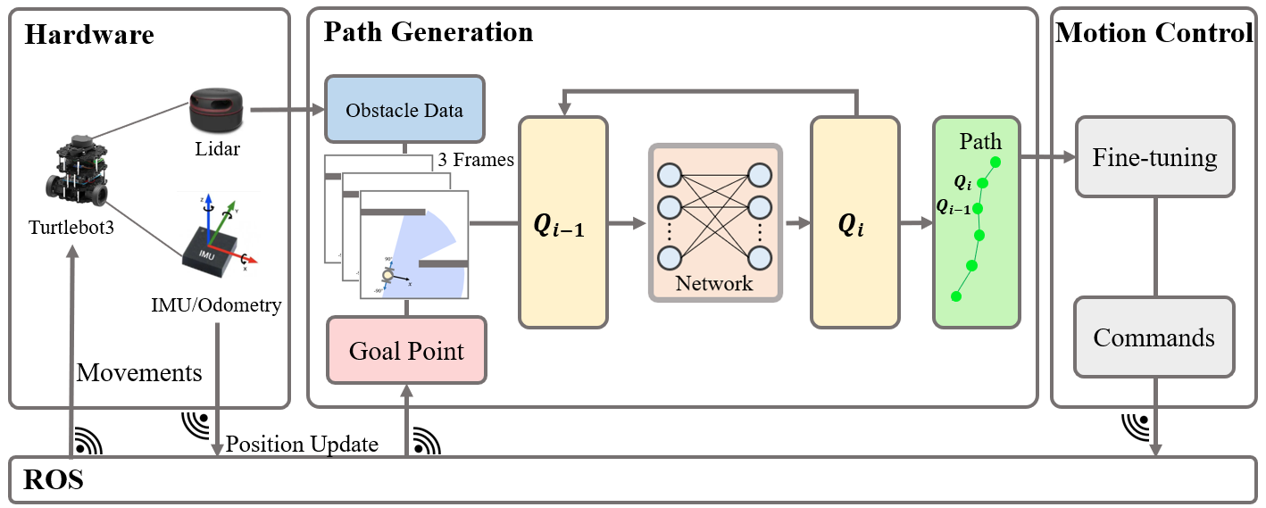
Figure 1: An overview of the framework. The obstacle data is collected by the lidar on Turtlebot3. The goal point is set up in advance. $Q_{i-1}$ and $Q_{i}$ represent the two adjacent path points. The network is a deep Markov model based policy network. During the robot movement, the path generation module dynamically generates multiple local paths based on varying sensor information and positions. The motion control module fine-tunes the paths and then sends execution commands to the robot.

Here we present a RL-based predictive path generation approach with fine-tuned motion control to drive the mobile robots in a variety of complex environments without any prior exploration while having only access to onboard sensors and computation. Different from other RL-based End-to-End approaches to output motion commands, we propose a novel RL-based method to generate predictive path points. This formulation could firstly fully utilize the advantages of learning-based methods such as fast inference speed and robustness to learn the mapping from raw sensor data to various types of outputs. Once a model is trained, substituting its controller in a modular way could fulfill navigation task requirements. Another great benefit is that our approach manages to decouple the trajectory generation and motion control since our RL-based approach’s action space and credit assignment are both based on planned trajectory, which means our path generation method is more robust to various environments.

Our novel actor policy based on the deep Markov model is designed for predictive path point generation. When generating paths, we fully consider the sequential relationship of adjacent path points. During the path generating process, the robot’s position, posture, and sensor information are dynamically changed. Due to robot kinematic limitations, the robot’s motion may not be consistent with the generated path, resulting in collision. Thus the motion fine-tuning module is proposed to fix the problem and improve safety. The overall framework is shown in Figure 1.

The main contributions of our work include:

• A RL-based path generation with fine-tuned motion control is proposed for robot’s navigation in an unknown environment without prior exploration. The path points prediction enables navigation and collision avoidance, while motion control is only used to ensure the safety of the robot in case of emergency.

• A novel deep Markov model trained by deep reinforcement learning to dynamically and iteratively predict planning path points. That is, at each time step, each predictive path point is obtained based solely on the previous path point and partially observable space, and we treat this point set as a planning trajectory. This predictive reinforcement learning based ‘action’ space later in simulation and experiments proves to be more optimal when the robot explores and navigates in unknown environments.

• Combining predictive path generation with control has the advantage of low coupling, allowing better differentiation between the two functions, and the role of each module on the robot will be well played.

II Related Work

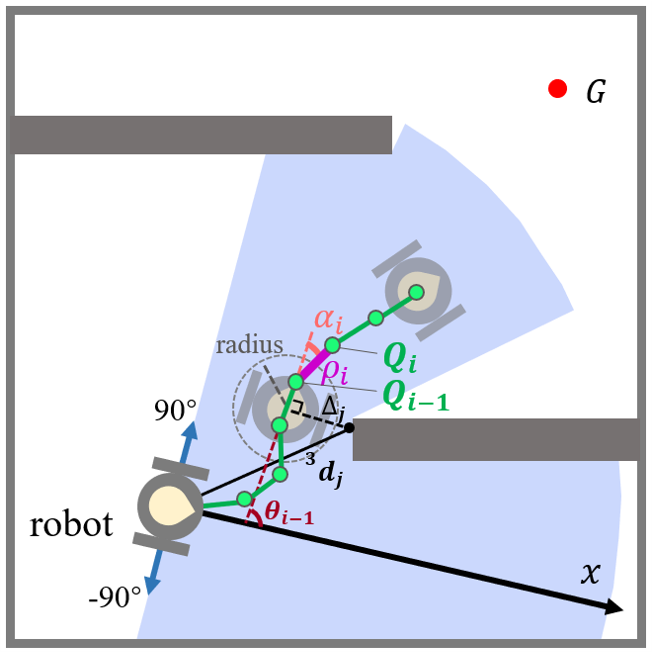
Figure 2: The blue sector is the obstacle data and the green points are the path points generated by the robot through the reinforcement learning method. $G$ represents the goal point. A plane rectangular coordinate system is established with the robot itself as the origin and x-axis denotes the robot’s facing direction. $\rho_{i},\alpha_{i}$ are the parameters of $Q_{i}$, which represents the distance the robot needs to travel and the angle that needs to rotate based on the $(i-1)^{th}$ path point $Q_{i-1}$. The ${}^{3}d_{j}$, defined in Equation 5 of Section IV, represents one of the obstacle data (distance between scanned obstacle and the lidar), while $\Delta_{j}$ represents the corresponding distance between the obstacle and the path.

For the representation of paths, the traditional approaches (e.g., [10]) are mostly points and line segments. Splitting the path into points and line segments is convenient for path expression and calculation. Traditional methods of path planning (e.g., [11, 3, 12]), typically generate a predicted segment of trajectory based on its state and convert it into executable instructions. As the number of predicted nodes increases, the computation time and resource consumption of the whole algorithm increase dramatically.

A number of path planning methods combined with learning algorithms require prior exploration of environments[13]. For example, the long-range path planning method (PRM-RL) [8, 9] uses a traditional method PRM for path planning of a globally known map, and then uses reinforcement learning method to generate robot’s actions for movement. RL-RRT[14], similar to PRM-RL, uses RRT algorithm to plan the global path and uses RL method to control robot’s motion for dynamic obstacle avoidance. Other grid-map-based methods such as PRIMAL[6], Improved DynaQ[15], RL-basd Heuristic Search[16], UAV-Path-Planning[17], etc., search for the higher scoring grids using learning algorithms in the grid map to form a path. Another approach uses Q-Learning[18] in the ANN method to plan the robot’s global moving direction, but switches to robot local planing module when it encounters an obstacle and guides the robot to change its direction to avoid collision.

Some other similar studies focus on using RL based method to generate the global path. In the known map, studies (e.g., [19, 20, 21]) present approaches based on RL that train networks with global information to generate all path points from the start point to the goal point once for the robots to follow.

Therefore, such RL-based approaches mentioned above focus on a prior exploration to the environment, planning the path and using reinforcement learning methods to regulate the robots’ movement actions. Instead, our approach focuses on utilizing reinforcement learning methods to make local path planning using obstacles information scanned by robot’s lidar without a map built in advance, and use fine-tuned motion control for robot movement.

Some other methods that do not require a prior exploration of the map, such as a local planner trained by RL[5, 1], only plan the robot’s motion instructions. PointGoal navigation, proposed in DDPPO[22], is used to infer the robot’s forward or rotation actions based on the images and GPS information using PPO method by giving robot the relative position of the target point. Here, the global map is of low importance and mainly assists the robot to locate the goal position.

III Problem Formulation

We here define how the robot’s path is expressed and transformed in the coordinate frames used in our approach. We use both an absolute world coordinate frame and a robot-relative local polar coordinate in our definition.

We use a set of points to represent a path. In the world coordinate system, the position and orientation of the robot is defined as $Qw(X,Y,\theta)$, where $X$, $Y$ represent the coordinates of the robot in the world coordinate system and $\theta$ represents the orientation of the robot. When converting $Qw$ into robot’s local polar coordinate $Q_{0}$, its local polar coordinates can be expressed as $Q_{0}(0,0)$. We define the robot’s facing direction as the direction of the x-axis in the robot’s local polar coordinate system. The orientation $\theta_{0}$ in polar coordinate at $Q_{0}$ is 0.

Then we define a generated path in the local coordinate as a set

$$L=\{Q_{i}(\rho_{i},\alpha_{i})|i\in(1,2,\dots,n)\}.$$ (1)

Here $\rho_{i}$ represents the displacement of $Q_{i}$ with respect to the previous point $Q_{i-1}$, $\alpha_{i}$ represents the angular deflection of $Q_{i}$ with respect to the previous point $Q_{i-1}$, shown in Figure 2.

In another word, $Q_{i}(\rho_{i},\alpha_{i})$ represents the predicted distance the robot needs to travel and the predicted angle the robot needs to rotate based on the $(i-1)^{th}$ path point $Q_{i-1}(\rho_{i-1},\alpha_{i-1})$ and the orientation $\theta_{i-1}$, shown in Figure 2. Here the orientation $\theta_{i}$ is accumulated by all $\alpha$.

$$\theta_{i}=\sum_{j=1}^{i}(\alpha_{j}).$$ (2)

We calculate the world coordinates of point $i$ using $\rho_{i}$, $\theta_{i}$ and its previous predicted point state $Qw_{i}(x_{i-1},y_{i-1},\theta w_{i-1})$. Here $x_{i-1}$ and $y_{i-1}$ are the world coordinates of previous points $Qw_{i-1}$, and $\theta w_{i-1}$ is accumulated orientation of all the previous points in the world coordinates. Specially, for the first point $Qw_{1}$, $x_{0}$, $y_{0}$ and $\theta w_{0}$ represent robot’s initial state.

When $i\geq 1$, for the $i^{th}$ point, we have

$$\begin{split}{x_{i}}={x_{i-1}}+{\rho_{i}}\cos({\theta w_{i}}),\\ {y_{i}}={y_{i-1}}+{\rho_{i}}\sin({\theta w_{i}}).\end{split}$$ (3)

So in the world coordinate we have

$$Lw=\{Qw_{i}(x_{i},y_{i},\theta w_{i})|i\in(1,2,\dots,n)\}.$$ (4)

We use the robot’s local coordinate system to generate the robot’s path point set $Q$ corresponding to itself and then transform the point set in the world coordinate for the controller to track.

For the goal point, we define it as $G(\rho_{g},\theta_{g})$ in the robot’s local polar coordinate. For the obstacle data, we use 180-dimensional obstacle data in 3 consecutive frames scanned by lidar.

IV Approach

IV-A Policy Representation

IV-A1 Observation Space

For each path point $Q_{i}$, the observation $\textbf{o}^{t}_{i}$ consists of three parts: the latest 3 frames of obstacle data $\textbf{o}^{t}_{d}$, the goal point $\textbf{o}^{t}_{g}$, and the previous point $Q_{i-1}$. Obstacle data is obtained from a rotating lidar sensor which returns distance to obstacles. Lidar is sampled every 1 degree from -90 degree to 89 degree with 0 degree as the robot’s forward heading. Three complete rotations of the lidar can then be combined into a history of three obstacle data readings as the obstacle data matrix $\textbf{o}^{t}_{d}$.

$$\textbf{o}_{d}^{t}=\begin{bmatrix}{}^{1}D\\ {}^{2}D\\ {}^{3}D\end{bmatrix},^{n}D=\{^{n}d_{i}|i\in[-90,90)\cap\mathbb{Z},n=1,2,3\}.$$ (5)

Here $i$ represents the $i^{th}$ angle divided equally by 180-degree from -90° to 89°, $n$ represents the $n^{th}$ frame of the obstacle data, and ${}^{n}d_{i}$ represents the distance between the lidar and the obstacle scanned on the angle $i$ in the $n^{th}$ frame. As the robot is moving, ${}^{n}D(n=1,2,3)$ are scanned at different positions and postures.

The goal point information needs to be transformed. We convert the goal point from the world coordinate to the local polar coordinate according to the goal point position $Gw(x_{gw},y_{gw})$ calibrated in the world coordinate system. We define the current state information of the robot mentioned in Section III as $Qw(X,Y,\theta)$. Here we have

$$x_{g}=(x_{gw}-X)\cos{\theta}+(y_{gw}-Y)\sin{\theta}.$$ (6)

$$y_{g}=-(x_{gw}-X)\sin{\theta}+(y_{gw}-Y)\cos{\theta}.$$ (7)

$$(\rho_{g},\theta_{g})=(\sqrt{x_{g}^{2}+y_{g}^{2}},\arctan(y_{g}/x_{g})).$$ (8)

Thus we have the goal information in local polar coordinate $\textbf{o}_{g}^{t}(\rho_{g},\theta_{g})$.

Therefore, the observation space $\textbf{o}^{t}$ consists of three parts.

$$\textbf{o}_{i}^{t}=(\textbf{o}_{d}^{t},\textbf{o}_{g}^{t},Q_{i-1}).$$ (9)

IV-A2 Action Space

In each cycle when generating a path, the path point $Q_{i}$ is one of the actions according to the data in the observation space and the network. Here the action space $\textbf{a}^{t}$ can be represented by $Q_{i}$. During the process of generating the path, all the actions are combined to be a complete path. According to the definition of the path in Equation 1, we have

$$\textbf{a}^{t}=\{Q_{i}|i\in(1,2,\dots,n)\}.$$ (10)

IV-A3 Reward Structure

We design the reward by judging the three elements of the path point. We call these three parts as

• $r_{c}$, if the predicted path collides with obstacles

• $r_{n}$, if the robot approaches the goal point

• $r_{s}$, smoothness judgment

The first is whether the generated path collides with the obstacle scanned by the lidar. We need to judge whether the path generated by the robot conflicts with the obstacles, as shown in Figure 2. For each frame of data swept by the lidar, we compute the scanned point and compute the distance $\Delta$ between the scanned point and the line segment connected by the path point. If $\Delta$ is less than the robot’s radius, it is judged as a collision.

$$r_{c}=\begin{cases}-15,\;break\quad&if\;\Delta_{i}<radius\;,\;i\in[-90,90)\cap\mathbb{N}\\ 0,\quad&otherwise.\end{cases}$$ (11)

If a collision occurs, we set $r_{c}=-15$, and terminate the training of the current process, which determines that the task failed.

For whether the path is approaching the goal, we compare the distance from the path points to the goal point and the distance from the robot to the goal point. For each point $i$, $s_{i}$ represents the distance between the $i^{th}$ path point and the goal point, and $d$ represents the distance between the robot and the goal point. If $s_{i}$ is smaller, the path point is closer to the goal, and the feedback is positive. Otherwise, it is negative. Thus

$$r_{n}=\sum_{i=1}^{n}(\frac{d-s_{i}}{i}).$$ (12)

For the smoothness judgment, if the second parameter $\alpha_{i}$ of the generated path points $Q_{i}(\rho_{i},\alpha_{i})$ is large, it means that the angle the robot needs to turn is large. Then, we can limit the size of the angle of each path point $\alpha_{i}$ to solve the problem of path smoothness. Thus, for all points in the path,

$$r_{s}=-\lambda\sum_{i=1}^{n}\alpha_{i}^{2},\lambda=0.0005.$$ (13)

Combining $r_{c}$, $r_{n}$ and $r_{s}$, we will obtain the total reward

$$r=r_{c}+r_{n}+r_{s}.$$ (14)

IV-A4 Actor-Critic Network

Our policy network is trained and inferenced in an iterable fashion. Given the input $\textbf{o}^{t}$ mentioned in Equation 9 and output $\textbf{a}^{t}$ mentioned in Equation 10, our policy could iteratively compute the mapping from observation space $\textbf{o}^{t}$ to action space $\textbf{a}^{t}$.

Note that not all observation space is observable. After the first iteration, path points are no longer obtainable. Only at the first iteration, our $Q_{i}$ as part of observation space is obtained directly as the point that represents the current robot location. For the rest of the iteration steps, we mark those unobservable positional points as ‘virtual’ position states that are generated by the previous iteration step, meaning the current single trajectory point depends on and only on partially observable environment space (in our space, lidar scan) and assume positional status at current iteration step which is exactly the output from the previous step. If $\pi$ represents the policy, we can generate all $Q$s from

$$Q_{i} \sim\pi(Q_{i}|(\textbf{o}_{d}^{t},\textbf{o}_{g}^{t},Q_{i-1}))$$

$$\sim\pi(Q_{i}|(\textbf{o}_{d}^{t},\textbf{o}_{g}^{t},\pi(Q_{i-1}|(\textbf{o}_{d}^{t},\textbf{o}_{g}^{t},Q_{i-2}))))$$

$$\sim\pi(Q_{i}|(\textbf{o}_{d}^{t},\textbf{o}_{g}^{t},\pi(\dots\pi(Q_{1}|(\textbf{o}_{d}^{t},\textbf{o}_{g}^{t},Q_{0}))))).$$ (15)

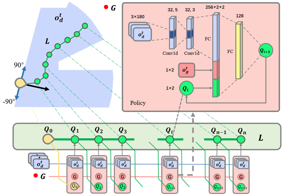
Figure 3: The architecture of the deep Markov model based policy network when generating path $L$. In the policy network, the inputs are the 3 frames of obstacle data $\textbf{o}_{d}^{t}$, local goal point $T$, and the previous point $Q_{i-1}$. It outputs current point $Q_{i}$. After $n$ times of point generation process, a complete path point set is presented. This process is then executed in a loop until the generation of $n$ path points is completed.

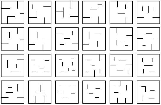
Figure 4: Training maps for 24 processes. The start points and the goal points are set randomly.

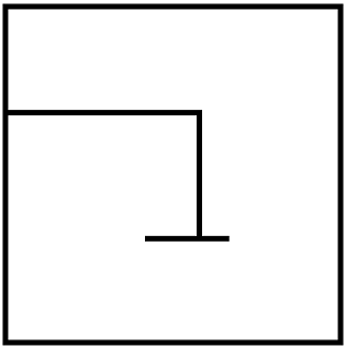
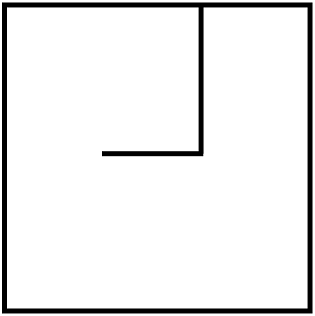
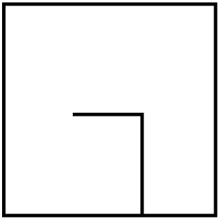
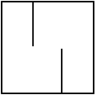
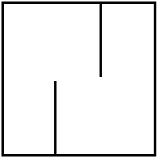
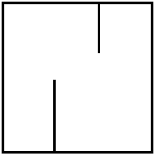
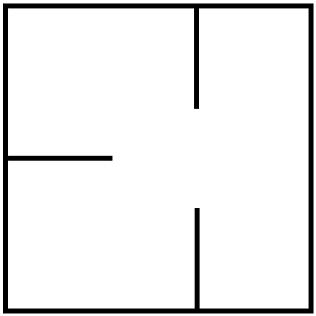
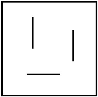
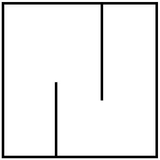
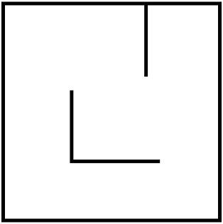
Figure 5: 10 testing maps. The size of each map is $6\times 6m^{2}$, expressed in the coordinate system as (-3, -3) to (3, 3). The robot is supposed to start from (-2, -2) and reach the goal (2, 2).

Our network shares the same weights and parameters at each iteration step. It is comprised of two convolutional layers to convolve 3*180 dimensional data $\textbf{o}_{d}^{t}$ to 1*256, then it is concatenated with other two inputs $\textbf{o}_{g}^{t}$ and $Q_{i-1}$ to form 260 (256+2+2) dimensional data. Then it comes through a fully connected layer that is added with leaky rectified linear units (ReLUs). The output of the network are variables: mean and standard deviation of Gaussian Distribution, as required by the PPO method to generate continuous and more diverse action space, followed by a sampling method thus to return final positional point as our action space. After all iteration steps are finished, our final action space as path points are obtained by concatenating all single-step action space, shown in Equation 10.

IV-B Training

For training, we refer to multi-process training approaches (e.g., [23, 24, 5, 6]) to improve the training efficiency. Multi-process Proximal Policy Optimization (PPO)[5] enables a multi-process update of the network. Twenty-four robots are trained in the corresponding maps (shown in Figure 4) and their start points and end points are set randomly. All policy training is done in simulation only.

In order to find the best path representation, we trained a number of different path generation networks. We tested the path with different number of path points $N$ and with different distance $\rho$ of adjacent path points to find out the best-fit path composition.

IV-C Motion Fine-Tuning

When the robot moves towards the target, the predicted points may be generated on both sides of robot at different time series, which may lead to shakes around predicted path. When the robot are too closed to an obstacle, if the shakes happens, the robot may crash into the obstacle. Thus to ensure the safety of the robot, a module is provided to fine-tune the robot’s motion instruction based on the predicted path points and the obstacle data, shown in Figure 6. We calculate the minimum value $F(i)$ in Equation 16 to find the execution direction. Here, we set $\alpha=0.3$ and $\beta=1.0$. $i$ represents one of the 180 obstacle data, and the max_range here represents the maximum sensor range and its value is 3.5m. ${}^{3}d$ is the 3rd latest obstacle data scanned by lidar, mentioned in Equation 5. $\psi$ represents the angle between direction $i$ and the first path point, shown in Figure 6.

$$F(i)=\alpha\sum_{j=i-5}^{i+5}(^{3}d_{j}-max\_range)^{2}+\beta\psi^{2}$$ (16)

$$i=\underset{i\in[-85,85)\cap\mathbb{N}}{{\arg\min}\,F(i)}$$ (17)

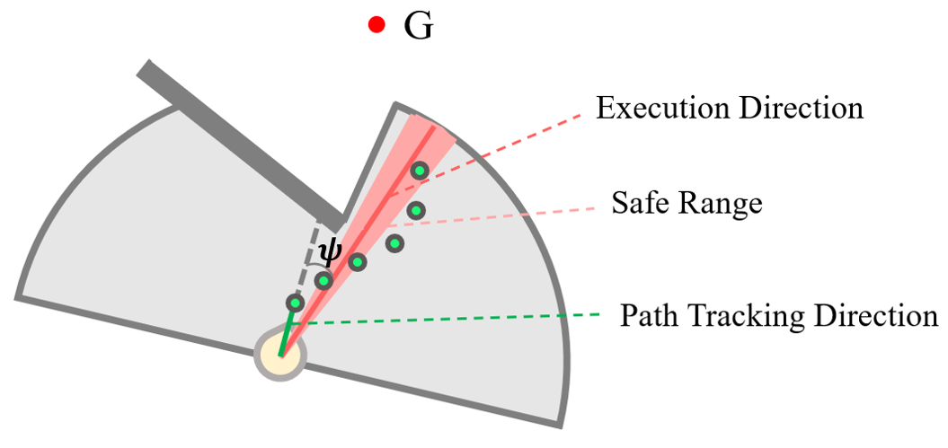
Figure 6: The motion fine-tuning module. Robot is supposed to follow the first predicted point generated by RL, which may lead to a collision if the direction is not safe. So the fine-tuning module is set to find a safe direction when generating the moving instructions for the robot. Execution Direction is selected by the minimum angle $\psi$ with the path tracking direction inside the Safe Range. The Safe Range here is a sector with an angle of 10 degree.

We record $i$ when $F(i)$ is minimal and regard it as the execution direction. Here $i$ is in the range [-85, 85) to ensure the value ${}^{3}d$ exists in Equation 16. Here we set the first point of the predicted path as the main moving direction. For the obstacle data scanned by lidar, if the obstacles are within 0.5m of the robot, the motion is fine-tuned to a direction away from the obstacles.

V Results and Discussion

We demonstrate that our proposed approach has a better structure than other approaches through comparative experiments. Meanwhile, we aim to find the best path structure by ablation experiments.

In our comparison experiments, we focus on the comparison with the DWA-RL approach proposed in [1] and traditional approach Artificial potential field (APF) approach[2, 25]. To compare the corresponding effects, the obstacle information acquisition of APF and DWA-RL approaches are adjusted accordingly in the experiment environments.

In the ablation experiments, we test the performance of different number of path points $N$ and the distance $\rho$ between adjacent path points.

V-A Evaluation Metrics

The following metrics are used to compare the performance of our approach with other approaches and to make further analysis in ablation studies.

• Average Trajectory Length - Average length of trajectory the robot travels from start point to goal point in the same test map.

• Time Cost - The average time cost from start point to goal point in the same test map.

• Success Rate - The rate of robot successfully travelling in an episode without any collision and finally reaching the goal. If a collision happens, the current test is immediately terminated and marked as failed.

V-B Comparison Experiments

V-B1 Simulation Experiments

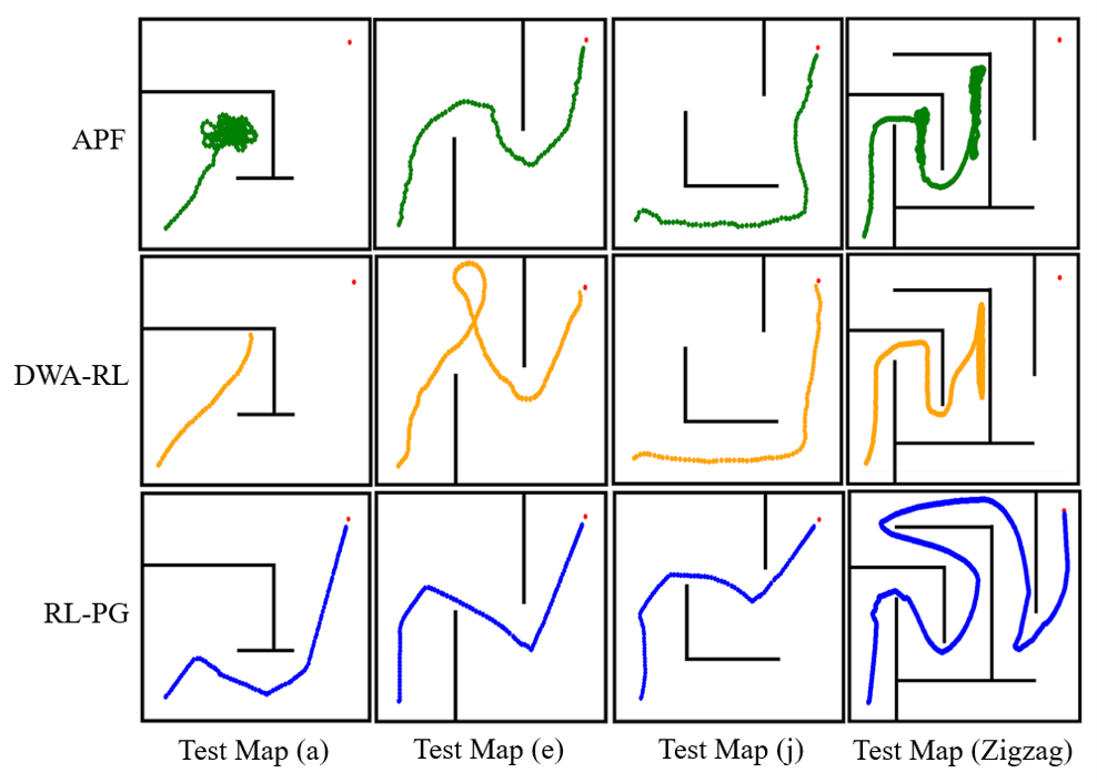
Figure 7: We compare our model with DWA-RL approach and APF approach in testing maps shown in Figure 5, and we take map (a), (e), (j) and a Zigzag test map to show the real trajectory driven by the robot. The red points represent the goal point in different maps. The green trajectories represent the trajectories drawn by robot with APF algorithm, the orange trajectories represent the trajectories drawn by robot with DWA-RL approach, and the blue trajectories represent the trajectories drawn by robot with our RL-based Path Generation (RL-PG) approach.

Metrics	Methods	Map a	Map b	Map c	Map d	Map e	Map f	Map g	Map h	Map i	Map j
Average Trajectory Length (m)	APF	$\infty$	6.071	12.008	5.328	11.223	6.419	5.444	5.781	22.027	7.372
	DWA-RL	$\infty$	6.178	$\infty$	5.386	11.419	8.470	5.430	7.206	12.619	6.901
	RL-PG	9.784	6.097	5.969	5.385	8.330	5.985	5.433	5.550	11.070	7.250
Average Time Cost ($\times$10s)	APF	$\infty$	6.620	12.508	5.971	11.658	7.066	6.156	6.402	22.340	7.862
	DWA-RL	$\infty$	6.681	$\infty$	5.938	12.093	8.697	5.938	7.561	13.187	7.231
	RL-PG	10.207	6.607	6.496	5.728	8.937	6.210	5.944	6.044	11.706	8.038
Success Rate (%)	APF	0	100	100	100	100	100	100	100	70	100
	DWA-RL	0	100	0	100	100	100	100	100	20	100
	RL-PG	100	100	100	100	100	100	100	100	100	100

TABLE I: Comparison Experiment Results

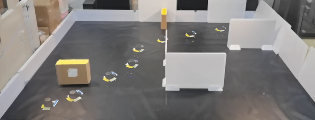
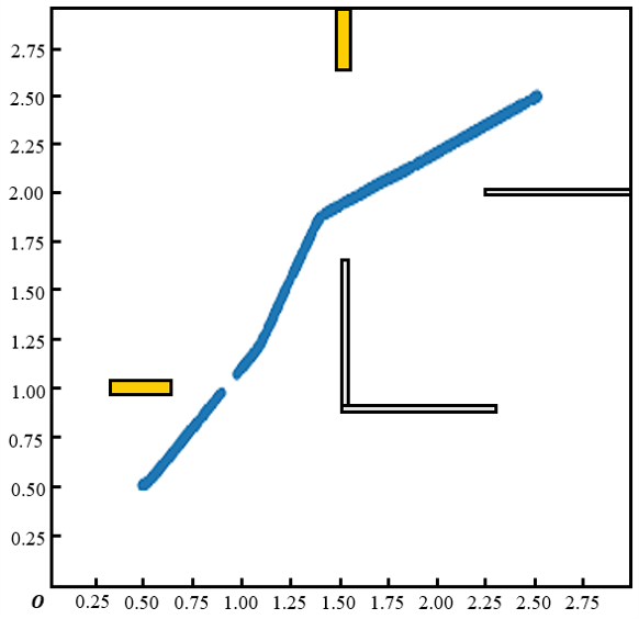
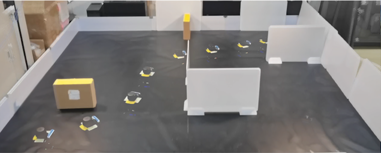
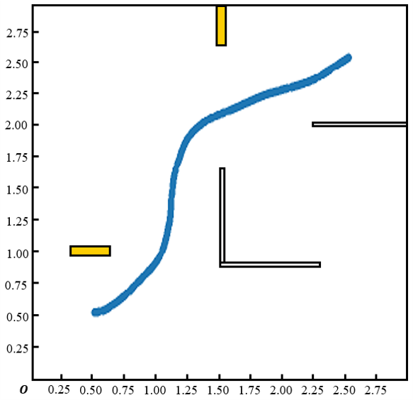
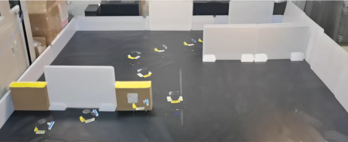
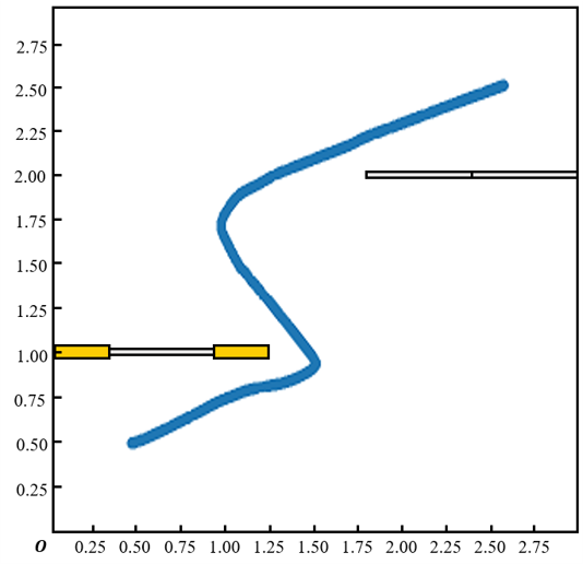
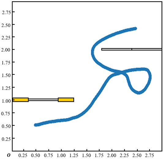
Figure 8: (a) and (e) are the real scenario screenshots of RL-PG approach while (b) and (f) are their corresponding trajectories. (c) and (g) are the real scenario screenshots of DWA-RL approach while (d) and (h) are their corresponding trajectories.

Metrics	$N$	$\rho$ (m)
		0.05	0.10	0.15	0.20	0.25	0.30
Average Trajectory Length (m)	3	5.93	6.02	6.00	6.04	5.92	5.90
	5	5.75	5.86	5.86	5.79	5.88	5.80
	10	5.65	5.69	5.70	5.68	5.66	5.63
	15	5.77	5.77	5.80	5.81	5.79	5.75
Average Time Cost ($\times$10s)	3	8.82	8.82	9.38	9.07	9.28	8.89
	5	7.45	7.68	7.60	7.48	7.78	7.60
	10	7.57	7.67	7.71	7.50	7.63	7.51
	15	10.93	11.84	11.76	12.24	11.52	11.69
Success Rate ($\%$)	3	100	100	100	100	100	100
	5	100	100	100	100	100	100
	10	100	100	100	100	100	100
	15	100	80	100	100	90	90

TABLE II: Ablation Experiment Results

We test our approach with DWA-RL approach[1] and APF approach[2, 25] on the same 10 testing maps shown in Figure 5 based on the simulator Stage. We trained our policy on a computer with one i7-8700 CPU and one Nvidia GTX 2080s GPU. The training of both our approach and the DWA-RL approach[1] runs $120000$ episodes. We take the testing maps (a)(e)(j) in Figure 5 and a Zigzag testing map as examples to show the trajectories robot travelled. Compared with other approaches, the trajectories of our approach are shorter, shown in Figure 7. We also found that when encountering certain situations, such as maze-like maps, the running time of the robot with DWA-RL and APF approaches increases significantly. But the robot with the path generation approach immediately finds a way to escape the maze and remove the deadlock situation caused by the environment.

In Zigzag testing map shown in Figure 7, we can see that the robot of the other approaches cannot find a feasible path over the wall when encountering corners and long walls, shown in Test Map (Zigzag) in Figure 7. Our approach can make better choices in the direction close to the goal point by exploring feasible paths in the same case. The DWA-RL approach and APF approach consumes a lot of resources to explore other feasible solutions with lower success rate when faced with the limitations of the complex environment.

Table I shows the detailed comparison results of the robot navigation tasks with different approaches. In test map (a), DWA-RL and APF approaches failed to find the goal due to the deceptive obstacles. In testing map (c) and (i), DWA-RL or APF also did not perform well. For trajectory length, our RL-PG approach are better in a deceptive map shown in Figure 7, while DWA-RL or APF approaches perform better in a simple environment. The max speed are all set 0.1m/s and we can find the RL-PG cost less time in most testing maps. As for the success rate, our RL-PG are all 100%, while DWA-RL and APF failed in some of the testing environments.

V-B2 Real Scenario Experiments

We designed physical experiments using Turtlebot3 robot with RPlidar_A2 on a $3\times 3m^{2}$ area and the data is communicated through ROS. We reduce the map size compared to the scene of the simulated environment.

Some experimental screenshots and their corresponding trajectories are shown in Figure 8. We found the pitfalls of the DWA-RL approach in real-world settings. In the real experimental scene, the DWA-RL approach trajectories are longer and the time costs are more than our approach as shown in Figure 8.

V-C Ablation Studies

In the simulation environment, we did ablation studies to observe the effects by the different distances $\rho$ between adjacent path points and different number of the path points $N$. We trained each model for 1000 episodes to compare the results. Here we recorded the test data shown in Table II. We take testing map (h) in Figure 5 as the test environment. From an overall perspective, when $N=10$ and $\rho=0.30$, the average trajectory length is minimum, and when $N=5$ and $\rho=0.05$, the average time cost is minimum. When $N$ is large, the success rate is lower.

We find that the performances of different distances between adjacent path points are close. The difference is that with smaller distances between adjacent path points, the network infers a higher probability of a predicted path that does not collide with an obstacle. The reason is that the larger the $\rho$, the easier the generated path is to conflict with the scanned obstacles. For $N$, when $N$ is small, the path points are more dispersed and require greater angular deflection in path tracking, which makes robot consume more time to turn a larger angle. However when $N$ is large, the time cost also increases and it takes more time to find the feasible, uncollide paths.

VI Conclusion

In this paper, we propose a novel RL-based robot path generation (RL-PG) approach with fine-tuned motion control. A deep Markov model suitable for path generation is trained using RL approach, which generates local paths in complex environments. The corrective effect of the controller is also able to correct the path generated by the deep Markov model to avoid collisions and improve the safety performance of the robot system.

With the experiments of comparing our approach with DWA-RL approach and traditional APF approach, we demonstrate that the RL-based path generation (RL-PG) with fine-tuned motion control is more effective and more safe. What is more, our approach is able to find feasible paths in a complex maze-like environment. In future work, we will try to apply the approach of path generation in the motion planning for multiple robots.

References

- [1] U. Patel, N. K. S. Kumar, A. J. Sathyamoorthy, and D. Manocha, “Dwa-rl: Dynamically feasible deep reinforcement learning policy for robot navigation among mobile obstacles,” in 2021 IEEE International Conference on Robotics and Automation (ICRA). IEEE, 2021, pp. 6057–6063.
- [2] Y. Chen, G. Bai, Y. Zhan, X. Hu, and J. Liu, “Path planning and obstacle avoiding of the usv based on improved aco-apf hybrid algorithm with adaptive early-warning,” IEEE Access, vol. 9, pp. 40 728–40 742, 2021.
- [3] M. Missura and M. Bennewitz, “Predictive collision avoidance for the dynamic window approach,” in 2019 International Conference on Robotics and Automation (ICRA). IEEE, 2019, pp. 8620–8626.
- [4] T. P. Nascimento, C. E. Dórea, and L. M. G. Gonçalves, “Nonholonomic mobile robots’ trajectory tracking model predictive control: a survey,” Robotica, vol. 36, no. 5, pp. 676–696, 2018.
- [5] T. Fan, P. Long, W. Liu, and J. Pan, “Distributed multi-robot collision avoidance via deep reinforcement learning for navigation in complex scenarios,” The International Journal of Robotics Research, vol. 39, no. 7, pp. 856–892, 2020.
- [6] G. Sartoretti, J. Kerr, Y. Shi, G. Wagner, T. S. Kumar, S. Koenig, and H. Choset, “Primal: Pathfinding via reinforcement and imitation multi-agent learning,” IEEE Robotics and Automation Letters, vol. 4, no. 3, pp. 2378–2385, 2019.
- [7] P. Cai, H. Wang, H. Huang, Y. Liu, and M. Liu, “Vision-based autonomous car racing using deep imitative reinforcement learning,” IEEE Robotics and Automation Letters, vol. 6, no. 4, pp. 7262–7269, 2021.
- [8] A. Francis, A. Faust, H.-T. L. Chiang, J. Hsu, J. C. Kew, M. Fiser, and T.-W. E. Lee, “Long-range indoor navigation with prm-rl,” IEEE Transactions on Robotics, vol. 36, no. 4, pp. 1115–1134, 2020.
- [9] A. Faust, K. Oslund, O. Ramirez, A. Francis, L. Tapia, M. Fiser, and J. Davidson, “Prm-rl: Long-range robotic navigation tasks by combining reinforcement learning and sampling-based planning,” in 2018 IEEE International Conference on Robotics and Automation (ICRA). IEEE, 2018, pp. 5113–5120.
- [10] X. Zhou, Z. Wang, H. Ye, C. Xu, and F. Gao, “Ego-planner: An esdf-free gradient-based local planner for quadrotors,” IEEE Robotics and Automation Letters, vol. 6, no. 2, pp. 478–485, 2020.
- [11] G. Bellegarda and K. Byl, “An online training method for augmenting mpc with deep reinforcement learning,” in 2020 IEEE/RSJ International Conference on Intelligent Robots and Systems (IROS). IEEE, 2020, pp. 5453–5459.
- [12] M. Ryll, J. Ware, J. Carter, and N. Roy, “Efficient trajectory planning for high speed flight in unknown environments,” in 2019 International conference on robotics and automation (ICRA). IEEE, 2019, pp. 732–738.
- [13] P. Anderson, A. Chang, D. S. Chaplot, A. Dosovitskiy, S. Gupta, V. Koltun, J. Kosecka, J. Malik, R. Mottaghi, M. Savva et al., “On evaluation of embodied navigation agents,” arXiv preprint arXiv:1807.06757, 2018.
- [14] H.-T. L. Chiang, J. Hsu, M. Fiser, L. Tapia, and A. Faust, “Rl-rrt: Kinodynamic motion planning via learning reachability estimators from rl policies,” IEEE Robotics and Automation Letters, vol. 4, no. 4, pp. 4298–4305, 2019.
- [15] M. Pei, H. An, B. Liu, and C. Wang, “An improved dyna-q algorithm for mobile robot path planning in unknown dynamic environment,” IEEE Transactions on Systems, Man, and Cybernetics: Systems, 2021.
- [16] X. Zhang, X. Kang, K. Wei, J. Li, and K. Ma, “Reinforcement learning combined with heuristic search for solving discrete space path planning problems,” in 2021 33rd Chinese Control and Decision Conference (CCDC). IEEE, 2021, pp. 2142–2147.
- [17] H. Bayerlein, M. Theile, M. Caccamo, and D. Gesbert, “Uav path planning for wireless data harvesting: A deep reinforcement learning approach,” in GLOBECOM 2020-2020 IEEE Global Communications Conference. IEEE, 2020, pp. 1–6.
- [18] Z. Ullah, Z. Xu, L. Zhang, L. Zhang, and W. Ullah, “Rl and ann based modular path planning controller for resource-constrained robots in the indoor complex dynamic environment,” IEEE Access, vol. 6, pp. 74 557–74 568, 2018.
- [19] H. Eslamiat, Y. Li, N. Wang, A. K. Sanyal, and Q. Qiu, “Autonomous waypoint planning, optimal trajectory generation and nonlinear tracking control for multi-rotor uavs,” in 2019 18th European control conference (ECC). IEEE, 2019, pp. 2695–2700.
- [20] P. Gao, Z. Liu, Z. Wu, and D. Wang, “A global path planning algorithm for robots using reinforcement learning,” in 2019 IEEE International Conference on Robotics and Biomimetics (ROBIO). IEEE, 2019, pp. 1693–1698.
- [21] J. Yu, Y. Su, and Y. Liao, “The path planning of mobile robot by neural networks and hierarchical reinforcement learning,” Frontiers in Neurorobotics, p. 63, 2020.
- [22] E. Wijmans, A. Kadian, A. Morcos, S. Lee, I. Essa, D. Parikh, M. Savva, and D. Batra, “Dd-ppo: Learning near-perfect pointgoal navigators from 2.5 billion frames,” arXiv preprint arXiv:1911.00357, 2019.
- [23] J. Schulman, F. Wolski, P. Dhariwal, A. Radford, and O. Klimov, “Proximal policy optimization algorithms,” arXiv preprint arXiv:1707.06347, 2017.
- [24] P. Long, T. Fan, X. Liao, W. Liu, H. Zhang, and J. Pan, “Towards optimally decentralized multi-robot collision avoidance via deep reinforcement learning,” in 2018 IEEE International Conference on Robotics and Automation (ICRA). IEEE, 2018, pp. 6252–6259.
- [25] Y. Huang, H. Ding, Y. Zhang, H. Wang, D. Cao, N. Xu, and C. Hu, “A motion planning and tracking framework for autonomous vehicles based on artificial potential field elaborated resistance network approach,” IEEE Transactions on Industrial Electronics, vol. 67, no. 2, pp. 1376–1386, 2019.