How Do the Probabilities Arise in Quantum Measurement?

Asatisfactory resolution of the persistent quantum measurement problem remains stubbornly unresolved in spite of an overabundance of efforts of many prominent scientists over the decades. Among others, one key element is considered yet to be resolved. It comprises of where the probabilities of the measurement outcome stem from. This article attempts to provide a plausible answer to this enigma, thus eventually making progress toward a cogent solution of the longstanding measurement problem.
Quanta 2021; 10: 65–74.

 
This is an open access article distributed under the terms of the Creative Commons Attribution License CC-BY-3.0, which permits unrestricted use, distribution, and reproduction in any medium, provided the original author and source are credited.

1 Introduction

The quantum measurement problem is considered as one of the important unresolved problems in physics although its origin goes back to the very inception of quantum mechanics nearly a century ago. In spite of an abundance of ideas that have been pursued throughout the decades resulting in countless articles, absence of a satisfactory explanation of the processes involved in the quantum to classical transition, also known as quantum measurement problem, has tenaciously persisted as a frustrating feature of quantum physics. This is very possibly because it involves the most distinctive characteristics of superposition of states in the quantum arena. A quantum state that has not yet been measured is in a superposition of two or more possible states of definite eigenvalue, the superposition differing qualitatively from any one of those states. There is no apparent manifestation of superposition in our familiar daily classical world, where tangible measurements of the quantum states are accomplished. In fact when we try to extrapolate the quantum superposition to classical domain in its entirety, we end up with such absurdity as the existence of a simultaneously dead and alive Schrödinger’s cat.

Yet it is an undeniable fact that the simultaneous existence of both the microscopic quantum world and the macroscopic classical world is essential for reality in a rather inseparably intertwined manner. For example, we humans are large and as such belong to the macroscopic classical world. However, everyone of us consists of about $7\times 10^{27}$ atoms [1] each containing additional elementary particles, all of which are in the microscopic quantum domain. Thus, we and everything else around us inevitably belong simultaneously both to the microscopic quantum as well as the macroscopic classical domain of the universe without ever paying much attention to this momentous reality. Indubitably the quantum realm does not exist somewhere out there. It is an essential part of our very existence. This inevitable transition from the quantum to classical domain taking place every moment of our life represents the basic premise of the quantum measurement problem. Significantly in recent times, experimental evidences conspicuously demonstrate that the distinctive phenomenon like quantum superposition just does not entirely disappear but inevitably get masked by interactions with the plethora of particles manifestly operational in the classical domain.

In a recent experiment, using a rather sophisticated procedure, coherent superposition has been demonstrated in a macroscopic object containing an estimated ten trillion atoms. For this purpose, the investigators [2] used a 40 micron long mechanical resonator, just large enough to be visible with the naked eye. The resonator with a resonant frequency of 6.175 GHz to its first excited phonon state was cooled to a temperature of merely 25 mK over absolute zero and put in a very high vacuum to minimize environmental effects. Under these circumstances, the resonator was confirmed to be in its ground state. Then a signal from a coupled qubit possessing the resonance frequency of 6.175 GHz was injected into the resonator thereby transferring the superposition feature of the qubit to the macroscopic object. Superposition of the ground and the first excited phonon state of the macroscopic resonator lasted for the resonator relaxation time of 6.1 ns.

The above demonstration provides strong evidence that quantum mechanics and its attendant aspect of superposition applies to macroscopic objects and can be revealed under appropriate circumstances provided that it was sufficiently decoupled from its environment. Can it apply to Schrödinger’s cat? The answer in principle should be yes. But to prove it, the cat will surely perish for other reasons! Because in order to conduct the experiment, it would be necessary to remove all sources of environmental disturbances exposing the cat to exceptionally low temperatures and high vacuum that would stop the metabolic processes for its survival. Further examples of coherence of superposition in large quantum objects have been presented by Bhaumik [3].

More recently, the quantum phenomena essentially arising from quantum fluctuations and superposition has been demonstrated in an as large an object as a man size 40 kg mirror in a gravitational detector [4]. The authors succinctly conclude, “It is remarkable that quantum vacuum fluctuations can influence the motion of these macroscopic, human-scale objects, and that the effect is measured.”

These experiments strongly point toward the fact that the quantum effects of the microscopic world is indeed present in the macroscopic domain but substantially veiled in their existence by the effects of some processes for the disappearance of the distinct quantum characteristics and the appearance of the classical world where we deal with an innumerable number of particles. Although substantial progress has been made, exactly how this is accomplished still comprises a subject of an overabundance of investigations with some intense debates. However, one particular aspect that is common to all these investigations is the scarcity of comprehension about where do the probabilities, rather than a certainty, in quantum measurement come from.

So far, only some ad hoc propositions such as Born’s rule [5] have allowed the physicists to predict experimental results with uncanny accuracy of better than a part in trillion [6]. But the basic cause of this essential rule has remained shrouded in a veil of mystery. One of the prominent investigators in this field, Wojciech Zurek has attempted to provide a derivation of the Born rule perhaps to make his program comprehensive [7]. But it has faced a stiff resistance from some foremost investigators including one of the giants of physics of our time, Nobel laureate Steven Weinberg.

In his classic textbook, Lectures on Quantum Mechanics, Weinberg states [8, p. 92], “There seems to be a wide spread impression that decoherence solves all obstacles to the class of interpretations of quantum mechanics, which take seriously the dynamical assumptions of quantum mechanics as applied to everything, including measurement.” Weinberg goes on to characterize his objection by asserting that the problem with derivation of the Born’s rule by Zurek “is clearly circular, because it relies on the formula for expectation values as matrix elements of operators, which is itself derived from the Born rule.” In [8, p. 26] he questions, “If physical states, including observers and their instruments, evolve deterministically, where do the probabilities come from? Again in his recent book [9, p. 131], Weinberg questions, “So if we regard the whole process of measurement as being governed by the equations of quantum mechanics, and these equations are perfectly deterministic, how do probabilities get into quantum mechanics?”

Maximilian Schlosshauer and Arthur Fine remark [10], “Certainly Zurek’s approach improves our understanding of the probabilistic character of quantum theory over that sort of proposal by at least one quantum leap.” However, they also criticize Zurek’s derivation of the Born’s rule of circularity, stating: “We cannot derive probabilities from a theory that does not already contain some probabilistic concept; at some stage, we need to “put probabilities in to get probabilities out.””

In this article, we present a plausible solution of the mysterious appearance of probabilities from some basic aspects of the well-established Quantum Field Theory (QFT) of the Standard Model of particle physics. Our argument relies on some characteristics of the universal quantum fields that appear to predetermine the values of the complex coefficients involved in the inherent superposition of eigenstates before measurement. Thus, it seems the century old mystery of quantum to classical transition could get a necessary boost from some recently revealed fundamental properties of the universe through the advent of QFT.

2 Significant characteristics of quantum fields

The ultimate ingredient of reality, uncovered by science so far, consists of fields, which are distinctively non-material in nature. Some perception of a field can be gained from our daily experience with the classical field of gravity that pervades us. The field that we do experience is stable everywhere in our vicinity but varies from place to place around its origin, the Earth. However, the ultimate realty of quantum fields also pervade all space including the one in which we exist, although we have no perception of them what so ever. Unlike the stable classical fields, however, the quantum fields are distinctly different in that they are incessantly teeming with intrinsic, spontaneous, and totally random activity all taking place locally in all space time elements, from the infinitesimal to the infinite everywhere in this unimaginably vast universe. Even though, we do not perceive its lively reality, indisputable evidence of its existence can be found everywhere in nature with the help of appropriate equipment. An outline of the salient features of the universal quantum fields are summarized below:

• Quantum fields are the primary ingredients of reality, from which all else is formed, fills all space and time.

• Every fragment, each spacetime element of the universe, has the same basic properties as every other fragment.

• “The deeper properties of the quantum field theory [$\ldots$] arise from the need to introduce infinitely many degrees of freedom, and the possibility that all these degrees of freedom are excited as quantum mechanical fluctuations.” [11, pp. 338-339].

• Thus the quantum fields are indeed alive with eternal, incessant, innately spontaneous, totally unpredictable activity of the quantum fields locally at each space time element even in perfect vacuum at absolute zero temperature.

• “Loosely speaking, energy can be borrowed to make evanescent virtual particles. Each pair passes away soon after it comes into being, but new pairs are constantly boiling up, to establish an equilibrium distribution.” [11, p. 404]

• One of the most notable aspects of the liveliness of the quantum fields is the fact that the expectation value or the average value of the quantum fields has remained immutable almost since the beginning of time in spite of its unique spontaneous random activities up to infinite dynamism.

Any reasonable concept of physical reality should then owe its eventual origin to the fundamental reality of quantum fields and their characteristic attributes. Of particular interest to us is to explore how the incessant, innately spontaneous and totally unpredictable activity of the primary reality of quantum fields comprising the overabundance of quantum fluctuations could foster the probabilistic nature of quantum states. All fundamental particles are inseparably intertwined in their existence with the quantum fields. Effects of the quantum fluctuations appear to have been generally underestimated even though matter would not have certain exceptional properties like the anomalous $g$ factor [12] and the Lamb shift [13] without them.

3 Wave function of an electron

The elementary particles like electrons, one of the initial products of material formation from the abstract but physical quantum fields, are quanta of the fields. However in reality, the physical electron state is actually a superposition of states produced by the interactions with the other fields of the standard model. But then the most significant question is, for a nonrelativistic single electron, what are these states that are superposed and how do they owe their existence to the interactions with the other fields? Are these really typical quantum states or just irregular disturbances in the field?

In order to give a physical depiction of the disturbances of the fields and quantum fluctuations, quoting from Frank Wilczek [14, p. 89]: “Here the electromagnetic field gets modified by its interaction with a spontaneous fluctuation in the electron field—or, in other words, by its interaction with a virtual electron-positron pair. [$\ldots$] The virtual pair is a consequence of spontaneous activity in the electron field. […] They lead to complicated, small but very specific modifications of the force you would calculate from Maxwell’s equations. Those modifications have been observed, precisely, in accurate experiments.” Emphasizing Wilczek’s critical observation again that in spite of the precipitous transitory characteristics of the virtual particles, there is an equilibrium distribution [11, p. 404].

Paraphrasing for further clarification, it turns out that the innately spontaneous activity of the electron field disturbs the electromagnetic field around them, and so electrons spend some of their time as a combination of two disturbances, one in in the electron field and one in the electromagnetic field. The disturbance in the electron field is not an electron particle, and the disturbance in the photon field is not a photon particle. However, the combination of the two is just such as to be a nice ripple, with a well-defined energy and momentum, and with an electron’s mass. This continues on and on, with a ripple in any field disturbing, to a greater or lesser degree, all of the fields with which it directly or even indirectly has an interaction. So we ascertain that particles are just not simple objects, and although we often naively describe them as simple ripples in a single field, that is far from true. Only in a universe with no spontaneous activities—with no interactions among particles at all—are particles merely ripple in a single field!

Would not it then be cogent to pronounce that the “states” being superposed here are the irregular disturbances of the fields originating from the incessant, innately spontaneous, and totally unpredictable quantum fluctuations? In fact we know quite explicitly what the states are out of which the physical electron is built, at least order by order in perturbation theory. The irregular disturbances of the fields indeed correspond to virtual particles. In particular, their respective energy-momentum does not correspond to the physical mass of a particle. One says that these particles are off-shell. However, in the process, the total energy-momentum is exactly conserved at all times. Because of the self-interaction of the quantum fields, such an energy-momentum eigenstate of the field can be expressed as a specific Lorentz covariant superposition of field shapes of the electron field along with all the other quantum fields of the Standard Model of particle physics.

It is particularly important to emphasize again that the quantum fluctuations are transitory but new ones are constantly boiling up to establish an equilibrium distribution so stable that their contribution to the screening of the bare charge provided the measured charge of the electron to be stable up to nine decimal places [15] (noteworthy, the elementary charge is no longer a measurable quantitity because it is exactly defined since 20 May 2019 by the International System of Units[16]) and the electron $g$-factor results in a measurement accuracy of better than a part in a trillion [6].

The Lorentz covariant superposition of fluctuations of all the quantum fields in the one-particle quantum state can be conveniently depicted leading to a well behaved smooth wave packet. A fairly rigorous underpinning of the wave packet function for a single particle QFT state in position space for a scalar quantum field has been provided by Robert Klauber [17]. Since particles of all quantum field are invariably an admixture of contributions from essentially all the fields of the Standard Model, the wave packet function of a single particle of a scalar quantum field can be considered to be qualitatively representative of those of the spinor and vector quantum fields as well.

Following Klauber, the wave function $\psi(x)$, for an electron in one dimension, can then be given by the Fourier integral

$$\psi(x)=\frac{1}{\sqrt{2\pi}}\int_{-\infty}^{+\infty}\tilde{\psi}(k)e^{\imath kx}dk$$ (1)

where $\tilde{\psi}(k)$ is a function that quantifies the amount of each wave number component $k=2\pi/\lambda$ that gets added to the combination.

From Fourier analysis, we also know that the spatial wave function $\psi(x)$ and the wave number function $\tilde{\psi}(k)$ are a Fourier transform pair. Therefore, we can find the wave number function through the Fourier transform of $\psi(x)$ as

$$\tilde{\psi}(k)=\frac{1}{\sqrt{2\pi}}\int_{-\infty}^{+\infty}\psi(x)e^{-\imath kx}dx$$ (2)

Thus the Fourier transform relationship between $\psi(x)$ and $\tilde{\psi}(k)$, where $x$ and $k$ are known as conjugate variables, can help us determine the frequency or the wave number content of any spatial wave function. A plot of the wave function $\psi(x)$ in equation (1) gives us the familiar wave function of a quantum particle like electron (Fig. 1).

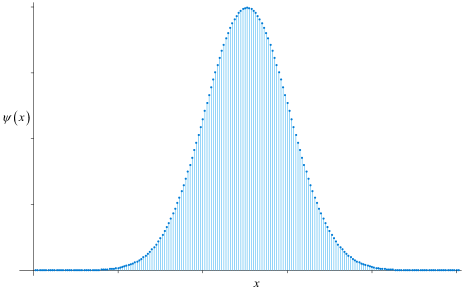
Figure 1: Plot of Gaussian wave packet function of an electron portrayed in equation (1) in position space. The amplitudes represent genuine reality as they correspond to the contributions from various quantum fields, the verified ultimate reality uncovered by science so far.

A few unique aspects of this depiction should be noted:

• First of all, the entire wave function as a whole represents all the requisite properties of the single electron. Therefore, in measurement, the entire wave packet should be acquired holistically or nothing at all. Experimental results demonstrate [18] that the entire extended wave packet can be reduced to the position of measurement instantaneously quite possibly because of the entanglement of the wave packet with the wave function of the quantum vacuum.

• The plot (Fig. 1) is a superposition of amplitudes as a function of position $x$. But what do these amplitudes represent? As we have repeatedly emphasized, these amplitudes arise from a mixture of different quantum fields even for a single quantum of the electron field. Consequently, they have nothing in common except energy, since the attributes of energy is the same irrespective of which quantum field they belong to. We are aware that these amplitudes do not constitute charge distribution of an electron as originally proposed by Schrödinger and shown to be incorrect by Born from his electron scattering experiments. But then what could these amplitudes mean?

4 Probability amplitudes

Following Einstein’s intuition, it would be cogent to consider that in measurement, a quantum particle would have the highest probability of being found where the intensity or the energy density of the quantum particle is the highest inside the wave packet. Energy density of a wave is given by the square of its amplitude. Therefore, to get the probability density, we have to take the square of the amplitude of the wave function, which usually involves a complex quantity. Consequently, the absolute square amplitude $\left|\psi(x)\right|^{2}=\psi^{*}(x)\psi(x)$, which is the probability density function $p(x)$, should represent the probability density for finding a particle in position space. Thus

$$p(x)=\left|\psi(x)\right|^{2}$$ (3)

Since the total probability is 1, the integral

$$\int_{-\infty}^{+\infty}\psi^{*}(x)\psi(x)dx=1$$ (4)

Max Born did something similar in formulating his famous Born’s rule. Quoting Born from his Nobel Lecture [19]: “Again an idea of Einstein’s gave me the lead. He had tried to make the duality of particles—light quanta or photons—and waves comprehensible by interpreting the square of the optical wave amplitudes as probability density for the occurrence of photons. This concept could at once be carried over to the $\psi$-function: $\left|\psi(x)\right|^{2}$ ought to represent the probability density for electrons (or other particles).” Since then it is known as the Born’s rule. However, Born could not have realized at his time that the wave function of the electron is derived from real quantum fields and therefore actually is real and so are the energy density amplitudes that can be described as probability amplitude, which consequently are real as well. It appears to be an erudite guess from Born’s part, especially judging from the fact that the single particle wave function was considered a fictitious mathematical construct at the time and the square of the wave function was added after submission of the original manuscript in 1926 [5] without any mention of energy density or intensity involved with wave functions. It is hard to imagine a fictitious mathematical construct having any energy density or intensity!

By now it should be evident that a quantum particle wave packet function is indeed real and far from being fictitious. Also Born’s rule can be reasonably derived following Einstein’s intuition and does not need to be a mere postulate. The fact that the position of the electron is given by a probability instead of certainty should not be surprising either. It is inevitable since the wave packet function is real. The Fourier transform correlations between conjugate variable pairs of any real wave packet have powerful consequences since these variables obey the uncertainty relation

$$\Delta x\Delta k\geq\frac{1}{2}$$ (5)

where $\Delta x$ and$\Delta k$ relate to the standard deviations $\sigma_{x}$ and $\sigma_{k}$ of the wave packet. This is a completely general property of a wave packet with a reality of its own and is in fact inherent in the properties of all wave-like systems. It becomes important in quantum mechanics because of the real wave nature of particles having the relationship $p=\hbar k$, where $p$ is the momentum of the particle. Substituting this in the general uncertainty relationship of a wave packet, the intrinsic uncertainty relation in quantum mechanics becomes

$$\Delta x\Delta p\geq\frac{1}{2}\hbar$$ (6)

It is thus evident that a particular fixed value of the position $x$ is not compatible with other measurable quantities like momentum.

However, it is critically important to note that whichever position $x$ turns up in the measurement process, its probability amplitude is predetermined from the complex interactions of the various quantum fields and encoded in the wave packet function. Again emphasizing from our earlier rather elaborate discussions, it should be aptly highlighted that the wave function is real and the computable value of the complex amplitudes $\psi(x)$ in the wave packet function is preordained from the indispensable interactions of the various quantum fields and their quantum fluctuations involved in the formation of the electron wave packet function.

For clarification, the wave number $k$ in the argument of the wave function for a massive particle like electron obeys the relativistic relation $p=\hbar k$. Therefore, for electrons $k$ in the exponent should be replaced by $p/\hbar$.

5 Probability in Hilbert space

It is of immense interest to emphasize again that the amplitudes in the wave packet of a particle resulting from the contributions of the diverse quantum fields are already predetermined. Hence the probability distribution of a quantum observable is already preordained before as well as after the unitary evolution of the Schrödinger equation. Can this comprehension be cogently extended to the observables in the customary Hilbert space formalism?

In Hilbert space, use of Dirac’s abstract algebraic model of bras and kets, from the bracket notation for the inner product, proved to be of great computational value. However, there were serious difficulties in finding a mathematical justification for using them in observables that have continuous spectrum as in the wave packet function of an electron we have been exploring so far. These difficulties were circumvented by the advent of the rigged Hilbert space (RHS) in 1960s [20, 21, 22]. The RHS is neither an extension nor an interpretation of the physical principles of Quantum Mechanics, but is simply a mathematical tool to extract and process the information contained in observables that have both continuous as well as discrete spectrum. Therefore, in spite of not using the Dirac’s bras and kets for the single particle, the inferences derived for the single particle wave packet can still be reasonably extended to the Hilbert space formalism. Observables with discrete spectrum and a finite number of eigenvectors (e.g., spin) do not need the RHS. For such observables, the Hilbert space is sufficient [22].

The Hilbert space is a square integrable, complex, linear, abstract space of vectors possessing a positive definite inner product assured to be a number. The states of a quantum mechanical system are vectors in a multidimensional Hilbert space containing an orthonormal basis set of eigenfunctions. The observables are Hermitian operators on that space, and measurements are orthogonal projections. The quantum wave functions, for example, the solutions of the Schrödinger equation describing physical states in wave mechanics are considered as the set of components $\psi(x)$ of the abstract vector $\Psi$, the state vector. However, the state vector does not depend upon any particular choice of coordinates. The same state vector can be described in terms of the wave function in position or momentum state or written as an expansion in wave functions $\psi_{n}$ of definite energy

$$|\Psi\rangle=\sum_{n}\psi_{n}|E_{n}\rangle$$ (7)

suggesting that every linear combination of vectors in a Hilbert space is again a vector in the Hilbert space. In general, the energy eigenstates $|E_{n}\rangle$ may not commute with the position eigenstates $|x\rangle$. The normalized square moduli $\left|\psi_{n}\right|^{2}$ of the energy complex coefficients are then interpreted as the probability for the system to be in the energy state $|E_{n}\rangle$ analogous to the single particle wave function where $\left|\psi(x)\right|^{2}$ is interpreted as the probability density for the particle to be at $|x\rangle$.

It is worthy to note that the coefficients $\psi_{n}(t)$ change during unitary time evolution but the probability for measuring outcome in a given energy eigenstate does not. The solution of the time-dependent Schrödinger equation is given by [23]:

$$|\Psi(t)\rangle=\sum_{n}\psi_{n}(0)e^{-\imath\frac{E_{n}}{\hbar}t}|E_{n}\rangle$$ (8)

where $E_{n}$ is the eigenvalue of the corresponding energy eigenvector $|E_{n}\rangle$. From (8), it is seen that for measurements in the energy basis the time dependence of $\psi_{n}(t)$ during unitary evolution drops out of the square modulus of the wave vector for computing the probability

$$\left|\psi_{n}(0)\right|^{2}e^{-\imath\frac{E_{n}}{\hbar}t}e^{+\imath\frac{E_{n}}{\hbar}t}=\left|\psi_{n}(0)\right|^{2}e^{0}=1\times\left|\psi_{n}(0)\right|^{2}$$ (9)

and the effective coefficient of superposition remains unchanged. Measurement in any non-commuting basis, however, leads to quantum interference effects of the $e^{-\imath\frac{E_{n}}{\hbar}t}$ terms [24, pp. 120-123].

Thus, it seems plausible that the gist of the ideas regarding the eventual origin of the probabilities from the incessant spontaneous activities of the ultimate reality of the quantum fields can be extended to the Hilbert space formalism. After all, Born’s rule was first derived historically for the single quantum particle and subsequently extended to the Hilbert space.

5.1 Projective measurement

Every vector in the Hilbert space, can be expressed in Dirac’s notation as a linear combination (7) of the energy basis vectors $|E_{n}\rangle$ with complex coefficients $\psi_{n}$. Multiplying both sides of (7) by $\langle E_{m}|$ gives

$$\langle E_{m}|\Psi\rangle=\sum_{n}\psi_{n}\langle E_{m}|E_{n}\rangle$$ (10)

Since

$$\langle E_{m}|E_{n}\rangle=\delta_{mn}=\begin{cases}1&\textrm{if }m=n\\ 0&{\textstyle\textrm{if }}m\neq n\end{cases}$$ (11)

it follows that

$$\psi_{n}=\langle E_{n}|\Psi\rangle$$ (12)

which is the transition amplitude of state $|\Psi\rangle$ to state $|E_{n}\rangle$. The energy basis vectors are then superposition of quantum states with complex coefficients if viewed in a different non-commuting basis.

Inserting (12) into (7) gives

$$|\Psi\rangle=\sum_{n}|E_{n}\rangle\langle E_{n}|\Psi\rangle$$ (13)

Further defining a projection operator $\hat{P}_{n}=|E_{n}\rangle\langle E_{n}|$ transforms (13) into

$$|\Psi\rangle=\sum_{n}\hat{P}_{n}|\Psi\rangle$$ (14)

leading to $\sum_{n}\hat{P}_{n}=\hat{I}$ signifying that the sum of all the projection operators is unity.

The outer product $|\psi\rangle\langle\psi|$ is called the projection operator since it projects an input ket vector $|\phi\rangle$ into a ray defined by the ket $|\psi\rangle$ as follows

$$|\psi\rangle\langle\psi|\,|\phi\rangle=|\psi\rangle\langle\psi|\phi\rangle$$ (15)

with a probability $\left|\langle\psi|\phi\rangle\right|^{2}$, as the inner product between two state vectors is a complex number recognized as the probability amplitude.

This is usually known as projective measurement and we should notice that it is important for the measurement of a mixed state consisting of an ensemble of pure states in a density matrix.

5.2 Operator valued observables

In a quantum system, what can be measured in an experiment are the eigenvalues of various observable physical quantities like position, momentum, energy, etc. These observables are represented by linear, self-adjoint Hermitian operators acting on Hilbert space.

Each eigenstate of an observable corresponds to eigenvectors $|\psi_{i}\rangle$ of the operator $\hat{A}$, and the associated eigenvalue $\lambda_{i}$ corresponds to the value of the observable in that eigenstate

$$\hat{A}|\psi_{i}\rangle=\lambda_{i}|\psi_{i}\rangle$$ (16)

For a Hermitian operator $\hat{A}$ , the quantum states associated with different eigenvalues are orthogonal to one another

$$\langle\psi_{i}|\psi_{j}\rangle=\delta_{ij}$$ (17)

The possible results of a measurement are the eigenvalues of the operator, which explains the choice of self-adjoint operators for all the eigenvalues to be real. The probability distribution of an observable in a given state can be found by computing the spectral decomposition of the corresponding operator. For a Hermitian operator $\hat{A}$ on an $n$-dimensional Hilbert space, this can be expressed in terms of its eigenvalues following (16) as

$$\hat{A}=\sum_{i}\lambda_{i}|\psi_{i}\rangle\langle\psi_{i}|$$ (18)

If the observable $\hat{A}$, with eigenstates $\left\{|\psi_{i}\rangle\right\}$ and spectrum $\left\{\lambda_{i}\right\}$ is measured on a system described by the state vector $|\Psi\rangle$, the probability for the measurement to yield the value $\lambda_{i}$ is given by

$$p\left(\lambda_{i}\right)=\left|\langle\psi_{i}|\Psi\rangle\right|^{2}$$ (19)

This again is the famous Born’s rule and we can see that it can be derived by extending the concepts discussed in the case of the single particle. After the measurement the system is in the eigenstate $|\psi_{i}\rangle$ corresponding to the eigenvalue $\lambda_{i}$ found in the measurement, which is called the reduction of state.

Recalling the discussions of the probability amplitudes in the one particle wave function, the probability amplitudes of the quantum states involved in superposition in Hilbert space has likewise been predetermined very possibly again because of the characteristic ceaseless activity and mutual interactions of the quantum fields. A quantum state in superposition generally has non-zero values for all states in superposition [9]. This is why we assert that the energy of the states is not on the mass shell. Again, this could be possible because of the interactions of the quantum states in superposition with the ceaseless quantum fluctuations just as in the case for the superposed components making up the composition of the structure of the non relativistic single electron.

It is of paramount importance to reemphasize that matter and particularly the elementary particles comprising them would not have some behavior in the absence of the special characteristics of the quantum fields listed earlier. These distinct activities are well recognized in the Lamb shift, anomalous electron $g$-factor, etc. Quantum superposition with definite complex amplitudes can therefore be also an example of such behavior.

5.3 Stern–Gerlach experiment

The Stern–Gerlach experiment is the most striking illustration of the experimental implementation of quantum measurements. It is as simple as it is persuasive. The following Stern–Gerlach experiment carried out using neutrons, each having a spin $\frac{1}{2}$, reinforces the fact that the probabilities of the eigenstates in superposition is present from the beginning, very likely because of the incessant activities of the quantum fields. The results of a series of Stern–Gerlach setups in tandem [25] show that the precise probabilities in superposition are indeed restored repeatedly following each projective measurement. After examining the results of these simple experiments, it is hard not be convinced about our assertion that the coefficients of probabilities are preexistent in superposition of states and their effect in the measurement of probability do not change during the unitary evolution of the superposed system.

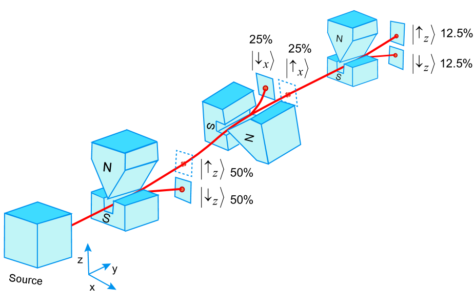
Figure 2: Serial Stern–Gerlach experiment in which neutrons are fired from a source into the non-homogeneous magnetic fields of three sequential Stern–Gerlach magnets oriented along the $z$-axis, the $x$-axis and the $z$-axis, respectively.

For the purpose of presentation clarity, we will assume that before entering the first Stern–Gerlach magnet (Fig. 2), the direction of the neutron spin magnetic moment is in a definite superposed state of two states referred to as spin-up and spin-down

$$|\Psi_{0}\rangle=\alpha|\uparrow_{z}\rangle+\beta|\downarrow_{z}\rangle$$ (20)

with unknown complex coefficients $\alpha$ and $\beta$ that are constrained by $|\alpha|^{2}=|\beta|^{2}=\frac{1}{2}$.

The superposed state (20) reduces (or collapses) as soon as the neutron enters the magnets of the analyzer to just one spin-$z$ direction by immediate momentum and energy transfer with the magnet, rather than by subsequent determination at the screen [26]. After exiting the magnet aligned in the $z$ direction, the trajectory of the neutron spin that can take only two equal but opposite values, will be deflected in either the $z+$ or $z-$ directions. If we denote these states by $|\uparrow_{z}\rangle$ and $|\downarrow_{z}\rangle$ respectively, we could say that the initial state performs one out of two equally probable quantum jumps

$$\begin{cases}|\Psi_{0}\rangle\to|\uparrow_{z}\rangle&\textrm{with }p=\frac{1}{2}\\ |\Psi_{0}\rangle\to|\downarrow_{z}\rangle&\textrm{with }p=\frac{1}{2}\end{cases}$$ (21)

When the beam of neutrons hits a detector screen, two spatially separated spots will appear corresponding to the two distinct trajectories. Each of the two spots would show equal number of neutrons following $|\alpha|^{2}=|\beta|^{2}=\frac{1}{2}$. If we now choose to send only the $|\uparrow_{z}\rangle$ state through second Stern–Gerlach magnet aligned in the $z$ direction, all the neutrons will be found, consistent with its preparation, in the upper region only.

However, if the state $|\uparrow_{z}\rangle=\frac{1}{\sqrt{2}}\left(|\uparrow_{x}\rangle+|\downarrow_{x}\rangle\right)$ faces Stern–Gerlach magnet aligned along the noncommuting orthogonal $x$-axis, any previous information about $|\uparrow_{z}\rangle$ will be completely destroyed and the direction of the spin magnetic moment will no longer be in an eigenstate of $\hat{\sigma}_{z}$ due to occurrence of one out of two equally probable quantum jumps

$$\begin{cases}|\uparrow_{z}\rangle\to|\uparrow_{x}\rangle&\textrm{with }p=\frac{1}{2}\\ |\uparrow_{z}\rangle\to|\downarrow_{x}\rangle&\textrm{with }p=\frac{1}{2}\end{cases}$$ (22)

Therefore, if only the $z+$ neutrons are passed through a second Stern–Gerlach magnet, which measures the neutron’s $x$-spins, the neutrons are deflected either right or left, labeled $x+$ and $x-$, and the number of neutrons with $|\uparrow_{x}\rangle$ and $|\downarrow_{x}\rangle$ spin is split even as expected.

Subsequently, if we pass only the $|\uparrow_{x}\rangle$ neutrons through a third Stern–Gerlach magnet oriented along the orthogonal $z$-direction, we observe that their previous $z$-spin value has been reset, and they are again split evenly between $z+$ and $z-$. This is despite the fact that we selected only the $z+$ neutrons from the first Stern–Gerlach magnet. When the second one is measured, it resets the state of the first one. Thus, there is another clear indication that the complex coefficients of superposition are predetermined, again very possibly by the quantum fluctuations. We can hence infer that the ceaseless quantum fluctuations as well as the mutual interactions of the quantum fields preordain the probability of detection of a quantum state.

In a recent investigation [27], by performing an ingenious experiment involving superposition of three eigenstates of a state vector given by

$$|\Psi\rangle=\alpha_{0}|0\rangle+\alpha_{1}|1\rangle+\alpha_{2}|2\rangle$$ (23)

it was strikingly demonstrated that the complex coefficient $\alpha_{0}$ governing the probability of the particular quantum state $|0\rangle$ in a superposition of three states can be measured without affecting the superposition of the two other remaining states in superposition. This further reinforces the fact that the coefficients of superposition that determines the probability outcome of measurement are predetermined.

6 Conclusion

History of the development of quantum mechanics is replete with a notable trend. Because of the sheer novelty of the subject so remarkably different from the established classical physics, the pioneers of the development of quantum physics utilized a procedure quite frequently with notable success. Due to a thorough lack of experience with the precepts of the newly emerging subject of quantum mechanics, an empirical model was fashioned first to accommodate the observed information. The experiential model was then amended to accommodate a more realistic version from a deeper understanding gained from subsequent revelations. This successful procedure started almost from the beginning with the proposal of a quantum by Max Planck.

Out of sheer frustration of not being able to match the characteristics of blackbody radiation to his equation, Planck introduced the indivisible radiation quantum believing it was just a necessary mathematical oddity without having any reality whatsoever. Five years later, Einstein persuasively demonstrated the reality of the quantum from the results of photo-electric effect. Citing another example, Neils Bohr crafted the first atomic model with discrete electron orbits merely to fit the observed spectral data. With the proposal and subsequent verification of matter wave, Schrödinger demonstrated Bohr’s discrete atomic orbits to be real standing wave patterns of matter wave and the list continues.

A similar situation presented itself with the fabrication of the wave packet function to accommodate the observed wave particle duality. It has essentially been considered to be a rather fictitious mathematical construct giving the probability density amplitude following Max Born’s educated guess. From our current deeper understanding based on contemporary knowledge of the primary reality of the quantum fields and their incessant, innately spontaneous, totally unpredictable activities identified as quantum fluctuations, we now realize that the wave packet function for a single nonrelativistic electron is in fact real. The wave function represents among others, real energy density amplitudes of the electron and consequently the probability density amplitude following Einstein’s intuition. Since the amplitudes of the wave function in position space are computable, the probability of the electron at a particular position is predetermined as a distinct result of the specific activities of the quantum fields. This phenomenon can be cogently extended to the superposition of quantum states in Hilbert space.

We, therefore believe that a plausible answer has now been provided to the question, where do the probabilities in the measurement come from, thus removing one of the hurdles in resolving the century old measurement problem.

References

- [1] B. Kross. How many atoms are in the human body?. Thomas Jefferson National Accelerator Facility - Office of Science Education 2021; https://education.jlab.org/qa/mathatom_04.html.
- [2] A. D. O’Connell, M. Hofheinz, M. Ansmann, R. C. Bialczak, M. Lenander, E. Lucero, M. Neeley, D. Sank, H. Wang, M. Weides, J. Wenner, J. M. Martinis, A. N. Cleland. Quantum ground state and single-phonon control of a mechanical resonator. Nature 2010; 464(7289):697–703. doi:10.1038/nature08967.
- [3] M. L. Bhaumik. Is Schrödinger’s cat alive?. Quanta 2017; 6:70–80. doi:10.12743/quanta.v6i1.68.
- [4] H. Yu, L. McCuller, M. Tse, N. Kijbunchoo, L. Barsotti, N. Mavalvala, et al.. Quantum correlations between light and the kilogram-mass mirrors of LIGO. Nature 2020; 583(7814):43–47. doi:10.1038/s41586-020-2420-8.
- [5] M. Born. Zur Quantenmechanik der Stoßvorgänge. Zeitschrift für Physik 1926; 37(12):863–867. doi:10.1007/bf01397477.
- [6] B. Odom, D. Hanneke, B. D’Urso, G. Gabrielse. New measurement of the electron magnetic moment using a one-electron quantum cyclotron. Physical Review Letters 2006; 97(3):030801. doi:10.1103/PhysRevLett.97.030801.
- [7] W. H. Zurek. Environment-assisted invariance, entanglement, and probabilities in quantum physics. Physical Review Letters 2003; 90(12):120404. doi:10.1103/PhysRevLett.90.120404.
- [8] S. Weinberg. Lectures on Quantum Mechanics. Cambridge University Press, Cambridge, 2013.
- [9] S. Weinberg. Third Thoughts. Harvard University Press, Cambridge, Massachusetts, 2018.
- [10] M. Schlosshauer, A. Fine. On Zurek’s derivation of the Born rule. Foundations of Physics 2005; 35(2):197–213. doi:10.1007/s10701-004-1941-6.
- [11] F. Wilczek. Fantastic Realities: 49 Mind Journeys and A Trip to Stockholm. World Scientific, Singapore, 2006. doi:10.1142/6019.
- [12] J. Schwinger. On quantum-electrodynamics and the magnetic moment of the electron. Physical Review 1948; 73(4):416–417. doi:10.1103/PhysRev.73.416.
- [13] W. E. Lamb, R. C. Retherford. Fine structure of the hydrogen atom by a microwave method. Physical Review 1947; 72(3):241–243. doi:10.1103/PhysRev.72.241.
- [14] F. Wilczek. The Lightness of Being: Mass, Ether, and the Unification of Forces. Basic Books, New York, 2008.
- [15] P. J. Mohr, B. N. Taylor, D. B. Newell. CODATA recommended values of the fundamental physical constants: 2006. Reviews of Modern Physics 2008; 80(2):633–730. doi:10.1103/RevModPhys.80.633.
- [16] D. B. Newell, E. Tiesinga. The International System of Units (SI). NIST Special Publication 330. National Institute of Standards and Technology, Gaithersburg, Maryland, 2019. doi:10.6028/nist.sp.330-2019.
- [17] R. D. Klauber. Student Friendly Quantum Field Theory. 2nd Edition. Sandtrove Press, Fairfield, Iowa, 2015.
- [18] M. Fuwa, S. Takeda, M. Zwierz, H. M. Wiseman, A. Furusawa. Experimental proof of nonlocal wavefunction collapse for a single particle using homodyne measurements. Nature Communications 2015; 6:6665. doi:10.1038/ncomms7665.
- [19] M. Born. Statistical interpretation of quantum mechanics. Science 1955; 122(3172):675–679. doi:10.1126/science.122.3172.675.
- [20] I. M. Gelfand, N. Y. Vilenkin. Generalized Functions, Volume 4: Applications of Harmonic Analysis. Academic Press, New York, 1964.
- [21] Y. M. Berezanskii. Expansions in Eigenfunctions of Selfadjoint Operators. Vol. 17 of Translations of Mathematical Monographs. American Mathematical Society, 1968.
- [22] R. de la Madrid. The role of the rigged Hilbert space in quantum mechanics. European Journal of Physics 2005; 26(2):287–312. arXiv:quant-ph/0502053. doi:10.1088/0143-0807/26/2/008.
- [23] L. Susskind, A. Friedman. Quantum Mechanics: The Theoretical Minimum. What You Need to Know to Start Doing Physics. Basic Books, New York, 2014.
- [24] D. D. Georgiev. Quantum Information and Consciousness: A Gentle Introduction. CRC Press, Boca Raton, 2017. doi:10.1201/9780203732519.
- [25] J. J. Sakurai, J. J. Napolitano. Modern Quantum Mechanics. Cambridge University Press, Cambridge, 2020. doi:10.1017/9781108587280.
- [26] M. Devereux. Reduction of the atomic wavefunction in the Stern–Gerlach magnetic field. Canadian Journal of Physics 2015; 93(11):1382–1390. doi:10.1139/cjp-2015-0031.
- [27] F. Pokorny, C. Zhang, G. Higgins, A. Cabello, M. Kleinmann, M. Hennrich. Tracking the dynamics of an ideal quantum measurement. Physical Review Letters 2020; 124(8):080401. doi:10.1103/PhysRevLett.124.080401.