Red supergiant stars in IC 1613 and metallicity-dependent mixing length in the evolutionary model

Abstract

We report a spectroscopic study on red supergiant stars (RSGs) in the irregular dwarf galaxy IC 1613 in the Local Group. We derive the effective temperatures ($T_{\mathrm{eff}}$) and metallicities of 14 RSGs by synthetic spectral fitting to the spectra observed with the MMIRS instrument on the MMT telescope for a wavelength range from 1.16 $\mu$m to 1.23 $\mu$m. A weak bimodal distribution of the RSG metallicity centered on the [Fe/H]=$-0.65$ is found, which is slightly lower than or comparable to that of the Small Magellanic Cloud (SMC). There is no evidence for spatial segregation between the metal rich ([Fe/H]$>-0.65$) and poor ([Fe/H]$<-0.65$) RSGs throughout the galaxy. The mean effective temperature of our RSG sample in IC 1613 is higher by about 250 K than that of the SMC. However, no correlation between $T_{\mathrm{eff}}$ and metallicity within our RSG sample is found. We calibrate the convective mixing length ($\alpha_{\mathrm{MLT}}$) by comparing stellar evolutionary tracks with the RSG positions on the HR diagram, finding that models with $\alpha_{\mathrm{MLT}}=2.2-2.4H_{P}$ can best reproduce the effective temperatures of the RSGs in IC 1613 for both Schwarzschild and Ledoux convection criteria. This result supports our previous study that a metallicity dependent mixing length is needed to explain the RSG temperatures observed in the Local Group, but we find that this dependency becomes relatively weak for RSGs having a metallicity equal to or less than the SMC metallicity.

1 Introduction

Red supergiants (RSGs) are massive stars with initial masses between about 9 $M_{\sun}$ and 30 $M_{\sun}$ at the post-main sequence evolutionary phase, of which the hydrogen envelopes are extended to several hundred solar radii (e.g., Levesque et al., 2005; Ekström et al., 2012). It is important to understand their physical properties such as the effective temperature, radius, and mass-loss rate in order to understand the evolutionary history of RSGs and the exact nature of Type II supernova progenitors.

The effective temperatures of RSGs are determined by the Hayashi limit (Hayashi, 1961). Stellar evolution models predict that this limit mainly depends on two factors for a given initial mass. One is metallicity, which greatly influences stellar opacity, and the other is the so-called mixing length, which characterizes the energy transport efficiency by convection in the convective hydrogen envelope (e.g., Elias et al., 1985; Ekström et al., 2012; Chun et al., 2018). The Hayashi limit shifts to a higher temperature for a lower metallicity and a larger mixing length (hereafter, the mixing length is denoted by $\alpha_{\mathrm{MLT}}$ which is given in units of the local pressure scale height $H_{P}$). The mixing length is a free parameter and needs an empirical calibration. Most stellar evolution models adopt a fixed mixing length of $\alpha_{\mathrm{MLT}}\approx 2.0$ following the calibration result with the Sun. However, some studies provide evidence that a fixed mixing length is not suitable for all types of stars (e.g., Guenther & Demarque, 2000; Bonaca et al., 2012; Tayar et al., 2017) and that the mixing length depends on metallicity for both low- and high-mass stars (Joyce & Chaboyer, 2018; Chun et al., 2018). More recently, González-Torà et al. (2021) also found that the standard solar mixing length is not applicable to RSGs in their comparison of effective temperature of Wolf-Lundmark-Mellote (WLM) galaxy with the Geneva evolution models.

Chun et al. (2018) calibrated the mixing length values in RSGs for various metallicities by comparing a grid of massive star evolution models with RSGs observed in the nearby universe, and found that the mixing length decreases for decreasing metallicity. Such a calibration of the mixing length is also important for theoretical predictions of the structure (in particular, the radius) of Type II supernova progenitors as discussed by Chun et al. (2018).

The effective temperatures of RSGs can be inferred from their spectra  (Levesque et al., 2005; Davies et al., 2013; Tabernero et al., 2018). However, spectroscopic studies on RSGs in the extragalactic galaxies are largely limited to the Magellanic Clouds (Levesque et al., 2006), M31 (Massey et al., 2009; Gordon et al., 2016), and M33 (Drout et al., 2012; Gordon et al., 2016). Only a small number of RSGs (about $10$ RSGs) in irregular galaxies with lower metallicity environments than the LMC metallicity have been investigated in several studies (Levesque & Massey, 2012; Britavskiy et al., 2014, 2015; Patrick et al., 2015; Garcia, 2018). Therefore, a spectroscopic investigation of a larger sample of RSGs in extragalactic galaxies with a wide range of metallicity from [Fe/H]$=-0.49$ (e.g., SMC) to [Fe/H]$=-1.0$ (e.g., Sextans A and Sagittarius Dwarf Irregular galaxy) would provide important information to constrain stellar evolution models of RSGs.

The photometric identification of RSGs for extragalactic galaxies (e.g., NGC 4449, NGC 5055, and NGC 5457 by Chun et al., 2017) including the dwarf irregular galaxy (dIrr) IC 1613 (Chun et al., 2015) has been conducted. IC 1613 is an excellent laboratory to study RSGs for a number of reasons. IC 1613 is a gas-rich, isolated galaxy with no past interaction with other galaxies. The distance of about 730 kpc (Dolphin et al., 2001; Pietrzyński et al., 2006), a low inclination of $i=38\arcdeg$ (Lake & Skillman, 1989) and the high Galactic latitude implying a low extinction value of $E(B-V)=0.02-0.04$ (Sandage, 1971; Freedman, 1988a; Cole et al., 1999) provide a great opportunity to access the resolved stellar populations with a reasonable exposure time from a ground-based telescope. Several studies indicate that IC 1613 has a nearly constant star formation rate over its entire lifetime (Cole et al., 1999; Skillman et al., 2003, 2014), hosting old ($>10$ Gyr), intermediate-age ($1-10$ Gyr), and young ($<$1 Gyr) stellar populations. However, most studies of the stellar populations in this galaxy have been focused on the old and intermediate-age stars having metallicity of [Fe/H]$=-1.75\sim-1.15$  (Cole et al., 1999; Tikhonov & Galazutdinova, 2002a; Skillman et al., 2003; Bernard et al., 2007; Skillman et al., 2014; Weisz et al., 2014; Chun et al., 2015; Sibbons et al., 2015; Pucha et al., 2019). The studies of the H II regions in this galaxy also indicate a low metallicity of 12+log(O/H) $\simeq 7.70$ (Kingsburgh & Barlow, 1995; Lee et al., 2003). Thus, IC 1613 is known to be an extremely low metallicity galaxy, being more metal-poor than SMC (Talent, 1980; Davidson & Kinman, 1982; Dodorico & Dopita, 1983; Peimbert et al., 1988; Herrero et al., 2010).

On the other hand, some studies on young stellar populations in IC 1613 imply different metallicity values. The studies on $3\sim 9$ O- and B-type supergiant stars in this galaxy give a metallicity of [Z]$=-0.82\sim-0.69$ (Bresolin et al., 2007; Garcia et al., 2014; Bouret et al., 2015). More recently,  Berger et al. (2018) found [Z]=$-0.69\pm 0.24$ with bimodal peaks at [Z]=$-0.50$ and [Z]=$-0.85$ for early B-type blue supergiants. Tautvaišienė et al. (2007) investigated the spectra of 3 M-type RSGs and found that the average metallicity is [Fe/H]=$-0.67\pm 0.09$. Britavskiy et al. (2019) investigated 6 RSGs including the RSG sample of Tautvaišienė et al. (2007). They adopted [Fe/H]=$-0.7$ for IC 1613 and found higher effective temperatures of RSGs than those of the SMC.

In this study, we investigate 14 RSG stars in IC 1613 using low-resolution $J$ band spectra obtained with the MMT and Magellan infrared spectrograph (MMIRS) on the 6.5 m MMT telescope. We aim to estimate the effective temperatures and metallicities of these RSGs, and calibrate the mixing length in stellar evolution models with our RSG sample. In Section 2 we describe the RSG target selection, observation and data reduction. In Section 3 we discuss the methods for determining the effective temperatures and metallicity. In Section 4 we compare the effective temperatures of our RSG sample with stellar evolutionary models and discuss its implications for the metallicity dependence of the mixing length. In Section 5 we conclude this work.

2 Target selection, observation and data reduction

RSG candidates are selected from the star catalog of IC 1613 classified by Chun et al. (2015). These authors investigated the stellar populations in IC 1613 using optical ($gi$) and near-infrared ($JHK_{s}$) photometry, and separated the stellar populations brighter than the tip of the red-giant branch (TRGB) into the Galactic foreground stars, supergiants, and asymptotic giant branch (AGB) stars in IC 1613 (see the text and Figure 4 in Chun et al., 2015, for details). In order to select suitable targets for MMIRS observation, we tested the slit mask configuration several times to maximize the number of observable RSGs considering the sky positions of the RSGs across the IC 1613 and distributions in the $(J-K_{s},K_{s})$ color-magnitude diagram (CMD). We finally select 72 targets among the 518 RSG candidates.

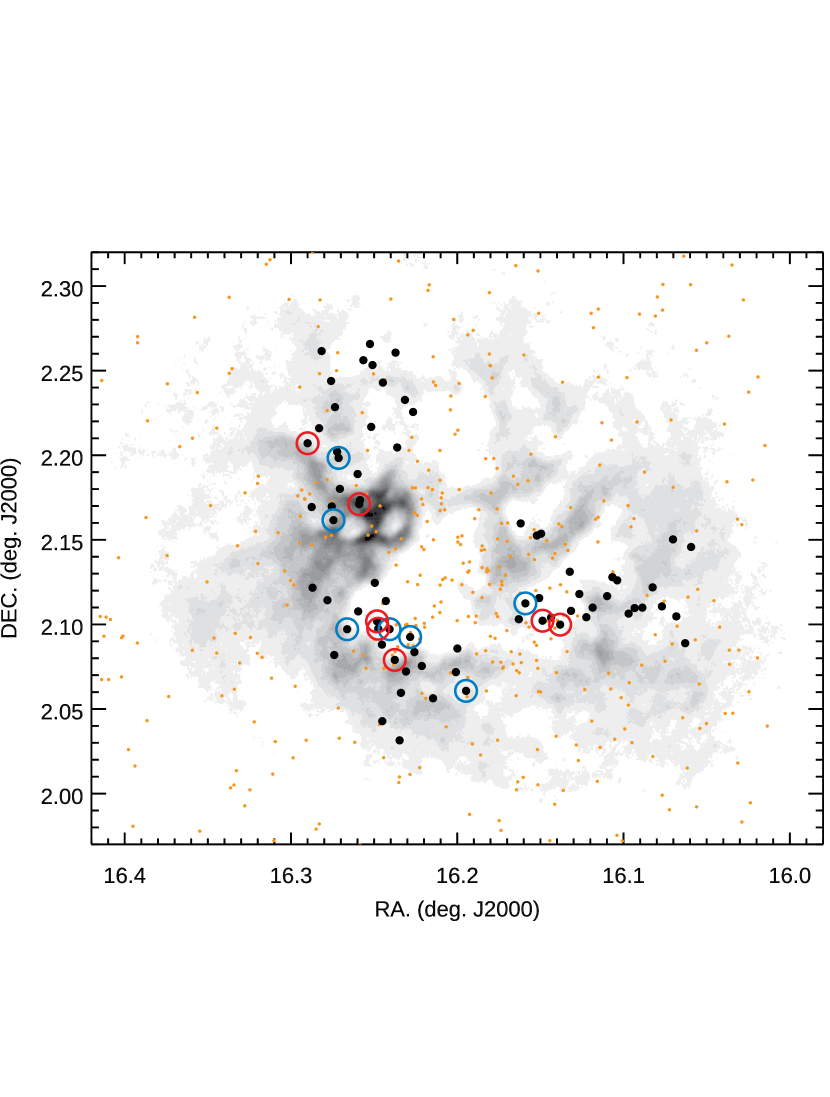
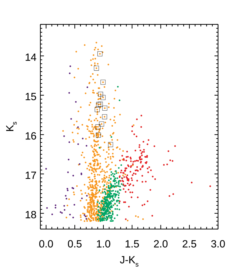
Figure 1: Left panel: The sky positions of the 518 RSG candidates (orange dots) classified by  Chun et al. (2015) and the 72 RSG candidates (black filled dots) observed in this study over the VLA H I map of Lozinskaya et al. (2001). The gray shading indicates H I column density: darker shading means higher density. The 14 RSGs of which the metallicity and effective temperature are inferred in this work are indicated by open circles, and the blue and red color of circles denote the metal poor ($\mathrm{[Fe/H]}<-0.65$) and rich ($\mathrm{[Fe/H]}>-0.65$) groups, respectively. Right panel: $(J-K_{s},K_{s})$ CMD of stars brighter than the tip of red-giant branch in IC 1613 (i.e., $K_{s}<18.2$ mag). The green and red dots denote M-giant and C-rich stars, respectively. The orange dots are the RSG candidates in IC 1613. The purple dots are foreground galactic stars. The open squares are the 14 RSG targets observed with the MMIRS for which the metallicity and effective temperatures are inferred in this work. The photometry data and stellar classification are taken from Chun et al. (2015).

In the left panel of Figure 1, the selected 72 RSGs candidates are displayed on the VLA H I map of IC 1613 (Lozinskaya et al., 2001). The RSGs in the central region of the galaxy having the H I cavity were not chosen because of the difficulty of the slit mask configuration due to the crowdedness. In the right panel of Figure 1, the $(J-K_{s},K_{s})$ CMD for several stellar populations in IC 1613 classified by Chun et al. (2015) is presented. The preselected RSGs have a wide magnitude range, from 13.5 mag to 18.0 mag in the $K_{s}$ band.

The near-infrared spectra for the 72 RSG targets have been obtained using the MMIRS instrument on the MMT telescope in the MOS mode. MMIRS has a HAWAII-2 $2048\times 2048$ HgCdTe detector with a pixel scale of $0.2^{\prime\prime}$, which covers a $4^{\prime}\times 7^{\prime}$ field of view in the MOS mode. The combination of $J$ grism and $zJ$ filter, which provides $J$ band spectra spanning $0.94-1.51$ $\mu$m, was used in the observation. Three slit masks with a slit width of 0.5 arcsec and a slit length of 7 arcsec to achieve a low-resolution of $R\sim 2000$ were created, following the MMT mask design procedure. The spectra data were acquired during the nights of September 1, 2 and 7 in 2017 by Queue mode. Our targets were observed using four dithering patterns with $\mathrm{+1.8}$, $\mathrm{-1.4}$, $\mathrm{+1.4}$, and $\mathrm{-1.8}$ arcsec offsets along the slit, and an individual exposure time of 300 seconds. We took three observation runs for each mask configuration to obtain enough signals. After the target observation, the telluric standard stars (A0V) for each mask were observed at a similar airmass to our target in order to correct for telluric absorption. The log of the observation is summarized in Table 1.

Table 1: Observation log for RSG candidates in IC 1613

Mask	RA.	DEC.	PA.	Exp. time
	(hh:mm:ss)	(dd:mm:ss)	(deg)	($N_{\mathrm{run}}\times N_{\mathrm{dith.}}\times$ sec.)
Mask1	01:04:58.56	02:05:12.43	42	$3\times 4\times$300
Mask2	01:05:02.17	02:12:41.71	-7	$3\times 4\times$300
Mask3	01:04:27.12	02:07:19.20	-96	$3\times 4\times$300

Data reduction was processed by using the MMIRS data reduction pipeline (Chilingarian et al., 2015) written in the IDL language. This pipeline automatically performs flat fielding, wavelength calibration, sky subtraction, and telluric correction using observed telluric standard stars for the MMIRS spectroscopic data. The final signal-to-noise ratios (S/N) per resolution element of the reduced spectra vary from 20 to 120, depending on the magnitudes of RSG candidates and the weather condition. We rejected the spectra with a S/N less than 40, and 33 RSG candidates with an average S/N$\simeq 80$ were preselected.

The radial velocities (RVs) for the 33 RSG candidates were measured by applying a cross-correlation technique to the observed spectra in the wavelength range from 1.15 $\mu$m to 1.25 $\mu$m, where several atomic absorption lines are present and the molecular lines are relatively rare. We use three template spectra, Betelgeuse and Arcturus from the NASA Infrared Telescope Facility spectral library for cool stars (Rayner et al., 2009), and a synthetic spectrum. The synthetic spectrum was generated by the local thermodynamic equilibrium (LTE) line analysis and synthetic spectrum code MOOG (Sneden, 1973) with a MARCS atmospheric model (Gustafsson et al., 2008) of $T_{\mathrm{eff}}=3800$ K, $\mathrm{log}$ $\mathrm{g}=-0.5$ and [Fe/H]=$-0.5$. We estimated RVs from the cross-correlation functions (CCF) between the observed and three template spectra, and the final RVs were averaged. From the resulting RVs, we find that 14 RSGs having an average RV of $-160~{}\rm km~{}s^{-1}$ are hosted in IC 1613. We note that it is difficult to precisely measure the RVs due to the low resolution and S/Ns of our spectra. The resulting RVs of $-160~{}\rm km~{}s^{-1}$ do not correspond to the systemic IC 1613 velocity of $-234~{}\rm km~{}s^{-1}$ measured from the H I 21 cm line spectra of Lu et al. (1993), but are in agreement with the value of $-185~{}\rm km~{}s^{-1}$ for RSGs in IC 1613 by Britavskiy et al. (2014).

3 Determination of stellar parameters

Table 2: Sky position, photometric magnitudes, and determined physical parameters of 14 RSGs in IC 1613

Star	RA.	DEC.	$J$	$H$	$K_{s}$	SN	$T_{\mathrm{eff}}$	log $g$	[Fe/H]	$v_{t}$	log L/L☉
	(hh:mm:ss)	(dd:mm:ss)					(K)			(km s-1)
star1	1:05:03.8905	+02:05:49.704	15.9264	15.2343	14.9763	120	4310$\pm$85 (4480)	0.9$\pm$0.2 (0.2)	-0.74$\pm$0.21 (-0.86)	4.0$\pm$0.4	4.629
star2	1:04:59.4095	+02:05:50.784	15.6624	14.9633	14.6693	120	4320$\pm$118 (4360)	0.8$\pm$0.3 (0.9)	-0.41$\pm$0.29 (-0.61)	3.9$\pm$0.6	4.729
star3	1:04:59.5798	+02:06:06.588	16.1524	15.4603	15.2353	100	4270$\pm$85 (4390)	0.9$\pm$0.1 (0.9)	-0.52$\pm$0.17 (-1.00)	3.9$\pm$0.4	4.544
star4	1:04:57.0190	+02:04:44.400	16.1744	15.5273	15.2283	110	4300$\pm$170 (4420)	0.9$\pm$0.4 (0.8)	-0.38$\pm$0.24 (-0.50)	3.1$\pm$0.4	4.531
star5	1:04:54.7993	+02:05:33.216	16.6994	15.9803	15.7313	100	4350$\pm$62 (4470)	0.6$\pm$0.7 (0.7)	-0.70$\pm$0.22 (-0.86)	3.7$\pm$0.4	4.317
star6	1:04:46.7303	+02:03:38.592	16.2564	15.5903	15.3643	100	4190$\pm$76 (4060)	0.6$\pm$0.4 (1.0)	-0.79$\pm$0.22 (-0.62)	4.3$\pm$0.4	4.507
star7	1:04:57.7702	+02:05:49.812	16.9254	16.2253	16.0133	90	4150$\pm$228 (4420)	0.7$\pm$0.6 (1.0)	-1.36$\pm$0.24 (-0.89)	3.1$\pm$0.6	4.236
star8	1:05:05.8704	+02:09:41.796	16.0504	15.3303	15.0573	40	4380$\pm$89 (4860)	-0.3$\pm$0.3 (-0.2)	-0.10$\pm$0.25 (-0.46)	3.9$\pm$0.6	4.574
star9	1:05:02.1506	+02:10:15.888	16.5674	15.8533	15.5473	40	4050$\pm$316 (4350)	-0.4$\pm$0.5 (0.6)	-0.36$\pm$0.32 (-0.78)	2.2$\pm$2.3	4.364
star10	1:05:09.6002	+02:12:25.488	14.8874	14.1993	13.9483	50	4370$\pm$85 (4370)	-0.4$\pm$0.4 (-0.5)	-0.58$\pm$0.23 (-0.85)	3.0$\pm$0.4	5.048
star11	1:05:05.1288	+02:11:54.312	15.1914	14.5893	14.3133	50	4360$\pm$88 (4570)	-0.3$\pm$0.4 (0.8)	-0.71$\pm$0.25 (-0.69)	3.9$\pm$0.4	4.937
star12	1:04:38.1697	+02:06:44.712	16.3524	15.6103	15.3283	50	4360$\pm$89 (4010)	-0.4$\pm$0.1 (0.7)	-1.02$\pm$0.24 (-0.75)	5.1$\pm$0.5	4.449
star13	1:04:33.1490	+02:05:59.496	16.7074	16.0013	15.8023	50	4360$\pm$105 (4140)	0.9$\pm$0.2 (0.6)	-0.59$\pm$0.26 (-0.72)	4.1$\pm$0.4	4.324
star14	1:04:35.6905	+02:06:07.884	17.3784	16.6543	16.2533	40	4120$\pm$117 (4400)	0.9$\pm$0.1 (0.9)	-0.50$\pm$0.25 (-0.69)	1.2$\pm$0.2	4.029

Inferring the effective temperature ($T_{\mathrm{eff}}$) is needed to understand the physical properties of RSGs and to confront the predictions of stellar evolution models, but it has been a challenging issue. Levesque et al. (2005, 2006) present comprehensive studies on the effective temperature of RSGs. They derive $T_{\mathrm{eff}}$ of RSGs in the Milky Way and the Magellanic Clouds by fitting the synthetic spectra generated with the MARCS atmosphere models to the TiO absorption band of the optical spectra. On the other hand,  Davies et al. (2013) estimate $T_{\mathrm{eff}}$ of RSGs in the Magellanic Clouds using the spectral energy distributions (SEDs), finding that $T_{\mathrm{eff}}$ inferred from the TiO band ($T_{\mathrm{eff,TiO}}$) is systematically lower than that from the SEDs ($T_{\mathrm{eff,SED}}$). Davies et al. (2013) argue that the TiO band property could not reflect the exact $T_{\mathrm{eff}}$ of the RSGs because the relatively upper layer of the atmosphere where the TiO band forms might be significantly affected by three-dimensional effects, such as granulation. Regarding the origin of the difference between $T_{\mathrm{eff,TiO}}$ and $T_{\mathrm{eff,SED}}$,  Davies & Plez (2021) recently suggest that the TiO absorption becomes stronger with presence of a strong wind, shifting the spectral type of a RSG to a later type for a given $T_{\mathrm{eff}}$. Alternatively atomic lines produced at a layer below the TiO band forming region would be less affected by the three-dimensional effects (Davies et al., 2013; Tabernero et al., 2018). Using atomic lines to infer $T_{\mathrm{eff}}$ and other stellar parameters of RSGs is investigated by several studies: CaT features (Dorda et al., 2016a, b; Tabernero et al., 2018; Dicenzo & Levesque, 2019), $J$-band technique (Gazak et al., 2014; Davies et al., 2015), and line-depth ratios of iron lines (Taniguchi et al., 2018, 2020). However, there are still some systematic offsets between the derived $T_{\mathrm{eff}}s$ from different methods.

In the present study, we apply the $J$-band technique to determine the stellar parameters of our RSG sample in IC 1613. We used the spectra ranging from 1.16 $\mu$m to 1.23 $\mu$m, where several atomic absorption lines (e.g., Fe, Mg, Si, and Ti) are present with little contamination by molecular lines, to apply the $J$-band technique discussed by Gazak et al. (2014) and Davies et al. (2015). To make a spectral fitting to the observed spectra, a synthetic spectra grid is generated using the online spectrum tool (Kovalev et al., 2018) hosted by the Max Planck Institute for Astronomy (MPIA), for which the RSG MARCS atmospheric models and the solar-scaled chemical abundance ratio from Grevesse et al. (2007) are used. The NLTE effects for several elements (e.g., Fe, Si, Ti, and Mg) are corrected (Bergemann et al., 2012, 2013, 2015). The grid covers a $T_{\mathrm{eff}}$ range of 3400 K $\sim$ 4400 K in increments of 100 K. The surface gravity of log $g$ ranges from -0.5 to +1.0 in increments of 0.5 (in cgs units), and the metallicity of [Fe/H] from -1.5 dex to +1.0 dex in increments of 0.25 dex. The microturbulence ($\xi$) range is from 1.0 km s^-1 to 6.0 km s^-1 in 1.0 km s^-1 increments.

The generated synthetic spectra are compared with the observed spectra, and stellar parameters and metallicity are determined by using $\chi^{2}$ minimization. As a first step, we fit the continuum level of both the observed and model spectra. We set wavelength points where any given synthetic spectrum within a 2–5 $\mathrm{\AA}$ wavelength window has a maximum flux, and we calculate the ratios of the model to the observed spectra flux at these wavelength points assuming the continuum level. The continuum correction function is then constructed by fitting the ratios with a low-order polynomial function. The outlier points with the residual of the fit larger than 3$\sigma$ are rejected. The final continuum correction function is applied to the synthetic spectra to fit the continuum level of the observation. At the same time, the synthetic spectra are also convolved to match the observed line profiles and the spectral resolution.

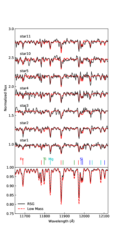
Figure 2: Top: Sample spectra of the observed RSG targets (black lines) with the best fit synthetic spectra (red lines). The prominent atomic lines are indicated by vertical lines. Bottom: The comparison between RSG model of 15$M_{\sun}$ (black) and low-mass model of 1$M_{\sun}$(red) spectra at low metallicity ([Fe/H]=$-0.7)$.

The $\chi^{2}$ values for all synthetic spectra are calculated, and the best model with the lowest $\chi^{2}$ value was selected. As investigated by Gazak et al. (2014), we keep two parameters among the four stellar parameters ([Fe/H], $T_{\mathrm{eff}}$, log $g$ and $\xi$) of the selected best model and investigate the $\chi^{2}$ distributions by varying the remaining two free parameters (e.g., [Fe/H] - $T_{\mathrm{eff}}$, [Fe/H] - log $g$, etc.). In this process, we can make six $\chi^{2}$ distribution planes with a combination of two different free parameters. For each of the six planes, we interpolate the $\chi^{2}$ grid of the two free parameters onto a denser grid plane and take two parameters at the minimum $\chi^{2}$ value as best fit values. Three best fit values for each stellar parameter were obtained from six $\chi^{2}$ planes. The final best fit parameters are averaged by these three values for each parameter. Figure 2 shows examples of the observed RSG spectra with the best fit synthetic spectra.

We estimate the uncertainties in deriving stellar parameters through Monte Carlo simulations. The synthetic spectra of the final best fit parameters are interpolated in the online spectrum tool with the correction of the NLTE effect. For each synthetic spectrum, we generate 200 noisy spectra by adding a random Gaussian noise to simulate the S/Ns of the observed spectrum. The best fit parameters of the individual noisy spectra are calculated through our analysis, and the distributions of the minimum $\chi^{2}$ for each parameter are investigated. The iso-contour levels, which encompass $1\sigma$ around a minimum $\chi^{2}$, are calculated, and then we take the minimum and maximum parameter values within the iso-contours to access $1\sigma$ uncertainty in stellar parameters. We summarize the fundamental physical parameters for the 14 RSG targets in IC 1613 in Table 2.

Although previous studies for RSGs in IC 1613 are limited, we compare our stellar parameters with the results of previous studies. We find that three RSGs (star4, star11, and star12) in our RSG targets are commonly detected in previous RSG studies: IC 1613-1 and IC 1613-3 in Britavskiy et al. (2019) and V43 in Tautvaišienė et al. (2007). The cross-identified RSGs in previous studies are indicated in the note in Table 2. We find that the average difference in the effective temperature ($\bigtriangleup T_{\mathrm{eff}}$) is about 350 K, which is so large that our results seem to be inconsistent with previous results. However, we note that Britavskiy et al. (2019) derived effective temperatures of RSGs using model SEDs with a fixed metallicity of [Fe/H]=$-1.0$ which is much lower than the metallicity measured in this study and Tautvaišienė et al. (2007), and also used narrow optical spectra with low S/N ratio which result in the significant uncertainties of the SED fitting.

3.1 Sensitivity test for RSG models, Signal-to-noise ratio, and spectral resolution

Figure 3: Top panels: The systematic offsets in metallicity (a) and temperature (b) obtained from low-mass spectra to RSG reference spectra at low metallicity ([Fe/H]=$-0.7$). The dotted lines are average offsets in metallicity and temperature and shaded area is $1\sigma$ error of average values. Bottom panels: The differences of metallicity (c) and effective temperature (d) between input and retrieved stellar parameters as a function of S/N per resolution elements and spectral resolution. The different resolutions are indicated by different colors: blue for R=2000, red for R=3000, and black for R=5000.

We found that the obtained effective temperatures of RSGs seem to be close to the edge ($\sim 4400$ K) of the model grid. The narrow grid coverage might introduce a bias into the results. A grid with a broader temperature range that fully encompasses the observed values is needed to obtain a more reliable result. Unfortunately, however, current available RSG models are limited up to $T_{\mathrm{eff}}=4400$ K temperature.

Regarding this problem,  Davies et al. (2010); Bergemann et al. (2012) noted that the model spectra between 1-5$M_{\sun}$ and 15$M_{\sun}$ for the same stellar parameters do not show much difference and there are small differences in NLTE abundance correction, according to which spherical MARCS models with lower mass instead of 15$M_{\sun}$ RSG models could be used to derive the stellar parameters of the RSGs. Contrary to the note of Davies et al. (2010); Bergemann et al. (2012), however, we found that there are considerable differences in the intensity of absorption lines between low-mass of 1$M_{\sun}$ and RSG of 15$M_{\sun}$ spectra at low metallicity (i.e., [Fe/H]=$-0.7$) across the $J-$band as shown in the bottom panel of Figure 2. The spectra of the low-mass star model show relatively stronger absorption lines than RSG spectra, which would lead to higher temperature and lower metallicity when we use the low-mass model spectra to fit the observed RSGs. Therefore, we calculate systematic offsets in temperature and metallicity in using low-mass models to derive RSG stellar parameters. Two sets of 100 RSG reference model spectra with $T_{\mathrm{eff}}=4000$ K and $4300$ K at IC 1613 metallicity were made, and then the stellar parameters of these spectra were estimated by using low-mass model spectra. The effective temperature range of $3500\leq T_{\mathrm{eff}}\leq 5000$ K and a fixed microturbulence ($\xi$) of 4.0 km s^-1 were used for model spectra.

In the top panels (a) and (b) in Figure 3, systematic offsets in metallicity and temperature obtained from low-mass models to the RSG reference spectra are plotted as a function of S/N ratios. We note that there is no a significant trend in the calculated systematic offsets between $T_{\mathrm{eff}}=4000$ K and $4300$ K RSG reference spectra. We find that the average temperature obtained from low-mass model spectra is systematically higher by about $130\pm 50$ K than that of reference RSG models, while the metallicity is lower by about $0.2\pm 0.1$ dex. This result is consistent with the predicted trend from using low-mass model, and corrections using these offset values should be applied to the stellar parameters obtained from the low-mass model spectra.

With the correction values, we use low-mass models and derive again the stellar parameters of the observed RSGs using the same fitting process. The stellar parameters after systematic corrections (i.e., $\triangle T=130$ K and $\triangle$ [Fe/H]$=0.2$) are indicated in the parenthesis in Table 2. The final corrected average temperature and metallicity (i.e., $\langle T_{\mathrm{eff}}\rangle=4380\pm 200$ K, $\langle\mathrm{[Fe/H]}\rangle$ = $-0.73\pm 0.15$) are comparable to those ($\langle T_{\mathrm{eff}}\rangle=4280\pm 110$ K, $\langle\mathrm{[Fe/H]}\rangle$ = $-0.68\pm 0.28$) obtained from RSG model spectra. We note that the average temperature and metallicity without corrections are higher by about 180 K and lower by 0.18 dex than those obtained from RSG model spectra, respectively. The differences in temperature and metallicity are almost consistent with the predicted systematic offsets. Therefore, we adopt and use the stellar parameters obtained from RSG models in the following analysis and figures.

Gazak et al. (2014) has tested the dependence of the inferred stellar parameters obtained by the J-band technique on the spectral resolution and S/N for the RSG spectra of solar metallicity, and shown that low resolution and/or low S/N can introduce systematic errors into the measured temperature and metallicity.  Gazak et al. (2014) suggested that the stellar parameters with reliable accuracy could be obtained from the RSG spectra with S/N $>$ 100 at the minimum spectral resolution of R=2000. Thus we also test the sensitivity of our stellar parameters as functions of spectral resolution and S/N. We made sets of 60 metal-poor ([Fe/H]= $-0.7$) RSG model spectra at given resolutions (R=2000, 3000, and 5000) and S/N per resolution elements (as 20, 40, 90, 130, and 170), respectively, and looked into how the retrieved stellar parameters compare to the input parameters. The average and standard deviation of the difference between the input and retrieved parameters were calculated.

The bottom panels (c) and (d) of Figure 3 show the differences of metallicity and effective temperature between input and retrieved parameters as functions of SN ratios and resolutions. The high-resolution spectra with a higher SN ratio provide more accurate effective temperatures with a small standard deviation. However, the temperature difference between the results with SN=40 and 100 at R=2000 is about 80 K, while the variation between the results with R=2000 and 5000 at SN=40 is about 40 K. In addition, the metallicity does not seem to be significantly changed by the resolution and SN ratio. For the spectral resolution (R=2000) and the SN ratio of our spectra, the maximum difference from the result of a higher resolution/SN ratio would be about 0.2 dex in metallicity and 150 K in temperature. Therefore we conclude that the resolution and SN ratio of our spectra can provide reasonable stellar parameters.

3.2 Metallicity and temperature distributions

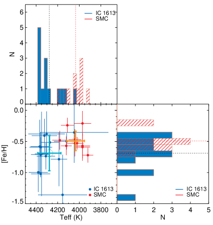
Figure 4: The effective temperatures of RSGs in IC 1613 as a function of metallicity. The RSG data in SMC given by  Davies et al. (2015) are also plotted with red dots. The mean metallicities and temperatures for IC 1613 and SMC are marked by cyan and orange open dots, respectively. The temperature and metallicity distributions are presented in the upper and right panels. The blue and red-hatched histograms are for IC 1613 and SMC, respectively. The black and red dotted lines in the distribution panels indicate the mean values for IC 1613 and SMC, respectively.

We present the metallicity and effective temperature of our 14 RSG targets in IC 1613 in Figure 4, compared with those of the RSGs in SMC given by Davies et al. (2015). The average metallicity of the RSG sample in IC 1613 is [Fe/H]=$-0.69\pm 0.27$, which is slightly lower than the average metallicity ([Fe/H]=$-0.49\pm 0.16$) of the SMC sample of Davies et al. (2015). This metallicity value is significantly higher than the metallicity of old and intermediate-age stellar populations in IC 1613  ($\mathrm{[Fe/H]}\sim-1.9$ to $-1.19$ Freedman, 1988b; Cole et al., 1999; Tikhonov & Galazutdinova, 2002b; Skillman et al., 2003; Kirby et al., 2013) but consistent with the young stellar population metallicity of [Fe/H]=$-0.69\pm 0.09$ (Tautvaišienė et al., 2007). Berger et al. (2018) also reports [Z]=$-0.69\pm 0.24$ for blue supergiant stars in IC 1613, which are RSG precursors. Since IC 1613 has been continuously star forming at a constant rate throughout its lifetime (Cole et al., 1999; Bernard et al., 2007; Skillman et al., 2014), the metal-richness of young stellar populations compared to old and intermediate-age stellar populations is expected, as also discussed in  Tautvaišienė et al. (2007).

One of the interesting results of Berger et al. (2018) is the bimodal metallicity distribution of blue supergiants and the spatial concentration of the metal-rich component in the central region of the galaxy. The metallicity distribution in our RSG sample shows a broad spread (see Figure 4). However, local peaks are also found at around [Fe/H]$\sim-0.4$ and [Fe/H]$\sim-0.7$, which are almost the same as those of Berger et al. (2018). Therefore, we divided the RSGs into two groups; 7 metal-rich ([Fe/H]$>-0.65$) and 7 metal-poor ([Fe/H]$<-0.65$). In the left panel of Figure 1, the metal-rich and metal-poor groups are indicated by red and blue open circles. Although the RSGs in the center of the galaxy were not observed in this study, there seems to be no spatial dependence between the metal-rich and metal-poor groups. Regarding the metallicity dependence, a non-significant (Sibbons et al., 2015) or slightly negative metallicity gradient (Chun et al., 2015) as a function of radial distance is reported for the intermediate-age AGB stars. Therefore, a study on metallicity of the RSGs in the central region or the H I cavity as well as metal-rich early A-type supergiants (ASGs) of Berger et al. (2018) is necessary to confirm the bimodal metallicity distribution and spatial dependence of RSGs.

Stellar evolutionary models predict systematically lower RSG effective temperatures at higher metallicity for a given mixing length (see Chun et al., 2018, for a recent discussion). In the effective temperature distribution of Figure 4, we find that the average temperature of RSGs in IC 1613 is higher (about 250 K) than that of RSGs in the SMC. Note, however, that no clear correlation between $T_{\mathrm{eff}}$ and metallicity among our RSG sample is found. The spectroscopic data with the higher resolution are necessary to find such a correlation among the RSGs in the galaxy. The trend of increasing temperature toward lower metallicity is also reported in the study of Britavskiy et al. (2019). They compared the effective temperatures of a small number of RSGs in several dwarf irregular galaxies (including IC 1613) having different metallicity environments in the Local Group, finding a clear trend of an increasing RSG effective temperature toward lower metallicity.

Our results appear to be in contrast to the previous work from Davies et al. (2013, 2015), who find roughly uniform temperature distribution of RSGs in the LMC and SMC. However, we have to note that they just find no systematic difference in temperature between the LMC ($4170\pm 170$ K) and SMC ($4030\pm 90$ K) for a small sample (9-10 RGSs) at the level of the precision of the measurements ($\sim 190$ K).  Davies et al. (2018) could later find a systematic shift in spectral types and temperature for a large sample of cool supergiants in LMC and SMC.  Tabernero et al. (2018) also find a significant difference ($\bigtriangleup T\sim 150$ K, see Figure 3 in their paper) in the temperature distributions between LMC and SMC for more than 400 RSGs. Although  González-Torà et al. (2021) could not find a meaningful difference in temperature between the LMC ($4140\pm 148$ K) and SMC ($4130\pm 103$ K) because of the rather large uncertainty ($\sim 180$ K) in their temperature measurement, they find that RSGs in the WLM dwarf galaxy, which has a lower metallicity than SMC, have a lower average $T_{\mathrm{eff}}$ than RSGs in SMC by about 250 K. Therefore, our finding that the average $T_{\mathrm{eff}}$ of RSGs in IC 1613 is higher than that of SMC RSGs supports the conclusion of  Davies et al. (2018),  Tabernero et al. (2018), and  González-Torà et al. (2021) that $T_{\mathrm{eff}}$ of RSGs increases with decreasing metallicity. A more accurate investigation of metallicity and temperature for a larger sample of RSGs in IC 1613 is needed to confirm the metallicity dependence of the RSG temperature in environments more metal-poor than the SMC.

4 Comparison with the stellar evolutionary tracks

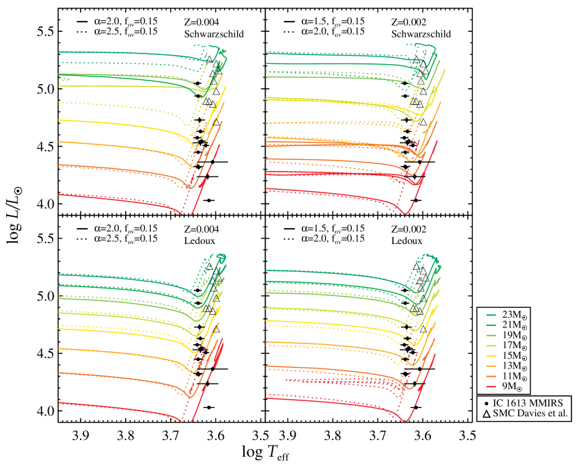
Figure 5: RSGs of IC 1613 on the HR diagram compared with the evolutionary tracks of SMC-like metallicity ($Z=0.004$, left panel) and $Z=0.002$ (right panel) with $f_{\mathrm{ov}}=0.15$, respectively. The Schwarzschild and Ledoux models are plotted in the top and bottom panels, respectively. The tracks with mixing lengths of $\alpha_{\mathrm{MLT}}=2.0$ (solid line) and $\alpha_{\mathrm{MLT}}=2.5$ (dotted line) are presented for $Z=0.004$, and those with $\alpha=1.5$ (solid line) and $\alpha=2.0$ (dotted line) for $Z=0.002$. The initial mass of each track is indicated by the color of the line. The RSGs in SMC from Davies et al. (2015) are indicated by open triangles.

We derive the bolometric luminosities of RSGs and compared the derived temperatures and luminosities with the evolutionary tracks in a Hertzsrung-Russel diagram (HRD). We use the near-infrared photometric magnitudes of Chun et al. (2015) in the $K$-band because the WIRCam photometry by Chun et al. (2015) provides more accurate magnitudes than those of the Two Micron All Sky Survey (2MASS, Cutri et al., 2003). The near-infrared magnitudes of WIRCam photometry are presented in Table 2. We note that the magnitudes of all RSG candidates of IC 1613 are on or below the limit of 2MASS. The bolometric magnitudes are calculated using the extinction values from Schlafly & Finkbeiner (2011), the bolometric correction relations between the $K_{s}$ band and $J-K_{s}$ for the spectroscopically late-type long periodic variables (Bessell & Wood, 1984), and the distance modulus of $\mu_{0}=24.291$ (Pietrzyński et al., 2006). This method is relatively insensitive to extinction as reported by Britavskiy et al. (2019). We also derived the bolometric luminosities using bolometric correction of Davies et al. (2013), and found that the average difference in both luminosities is about 0.005 dex.

The evolutionary tracks to compare with our RSG targets are calculated with the MESA code (Paxton et al., 2011, 2013, 2015). We follow the same physical assumptions described in Sect. 2 of Chun et al. (2018). In short, we considered both the Schwarzschild and Ledoux criteria for convection. Since the average metallicity of RSGs in IC 1613 is comparable to or slightly lower than that of SMC, we calculate the evolutionary tracks of the SMC-like ($Z=0.004$) and lower ($Z=0.002$) metallicities. For each metallicity, four different mixing length parameters: $\alpha_{\mathrm{MLT}}=1.5,2.0,2.5$ and $3.0$, which are given in units of the local pressure scale height, are considered. An overshooting parameter of $f_{\mathrm{ov}}=0.15$, which is given in units of local pressure scale height at the upper boundary of the convective core, is used.

In Figure 5 we present the RSGs of IC 1613 on the HR diagram compared with the evolutionary tracks at $Z=0.004$ and $Z=0.002$. We also include the RSGs in the SMC of Davies et al. (2015) in the figure. As discussed in Chun et al. (2018), the evolutionary tracks of $Z=0.004$ with about $\alpha_{\mathrm{MLT}}=2.0$ for both the Schwarzschild and Ledoux criteria can reproduce the temperatures of the RSGs in the SMC. However, these tracks are systematically cooler than the temperatures of the RSGs in IC 1613. The evolutionary tracks with $\alpha_{\mathrm{MLT}}=2.5$ are roughly compatible to the positions of the RSGs of IC 1613. For $Z=0.002$, the evolutionary tracks with $\alpha_{\mathrm{MLT}}=2.0$ give effective temperatures consistent with those of observed RSGs in IC 1613.

The average luminosity of our RSG targets in IC 1613 is lower than that of the SMC. The majority of RSGs in IC 1613 are located below the 19M_☉ evolutionary track (Figure 5). This is simply because of the selection effect in our work. As shown in the CMD of Figure 1, the majority of the observed RSGs in IC 1613 have a magnitude of $K_{s}>15$, and there are many bright RSG candidates that are not observed in this study. If we had a larger sample of RSGs including bright candidates over the full spatial extent of IC 1613, it would be possible to constrain the $L_{\mathrm{max}}$ or the Humphreys-Davidson limit in this galaxy.

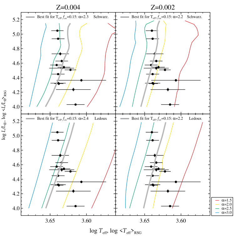
Figure 6: RSGs of IC 1613 on the HR diagram compared with the time weighted temperatures and luminosities of the evolutionary tracks with metallicities of Z=0.004 (left panel) and 0.002 (right panel). The Schwarzschild and Ledoux models are plotted in the top and bottom panels, respectively. The time-weighted values of tracks for different mixing lengths ($\alpha_{\mathrm{MLT}}=1.5,2.0,2.5,$ and $3.0$) are indicated by red, yellow, green, and cyan lines, respectively. The best fits to the derived effective temperatures of RSGs in IC 1613 are represented by thick gray line and the mixing length that gives the best fit is indicated by the label in the upper part of each panel.

In order to find the mixing length value that gives the best fit to the position of RSGs in the HR diagram, the time-weighted effective temperature ($<T_{\mathrm{eff}}>_{\mathrm{RSG}}$) and luminosity ($<L>_{\mathrm{RSG}}$) from the evolutionary tracks are calculated. We interpolate $<T_{\mathrm{eff}}>_{\mathrm{RSG}}$ and $<L>_{\mathrm{RSG}}$ at mixing lengths from $\alpha=1.5$ to 3.0 in increments of 0.1, and then compare the effective temperatures of the RSGs in IC 1613 with those of the interpolated values at a given luminosity. The $\chi^{2}$ value is calculated from the deviation between the observation and model temperatures, and the mixing length value with the lowest $\chi^{2}$ is selected as the best fit value (see Sect. 4 of Chun et al., 2018, for more details on this approach.).

In Figure 6, the effective temperatures and luminosities of the RSGs in IC 1613 are compared with time-weighted temperatures and luminosities of the evolutionary tracks in the HR diagram. From our $\chi^{2}$ minimization analysis, we find that the best fits of the Schwarzschild and Ledoux models with $Z=0.004$ to the observation are given by $\alpha_{\mathrm{MLT}}=2.3$ and $2.4$, respectively. On the other hand, for $Z=0.002$, a lower mixing length value of $\alpha_{\mathrm{MLT}}=2.2$ for both the Schwarzschild and Ledoux models gives the best fit to the observed data.

Figure 7: The calibrated mixing length values of WLM (Z=0.0014), IC 1613 (Z=0.002 and 0.004), SMC (Z=0.004), LMC (Z=0.007) and the Milky Way (Z=0.02) (Chun et al., 2018) as a function of metallicity obtained with the Schwarzschild (upper panel) and Ledoux (lower panel) models. The mixing length values of SMC, LMC, and the Milky Way calibrated by $f_{\mathrm{ov}}=0.15$ models and SED temperatures were adopted.

In Figure 7, we compare the mixing length value of IC 1613 with those of the SMC (Z=0.004), LMC (Z=0.007), the Milky Way (Z=0.02) from Chun et al. (2018). We assume Z=0.002 and Z=0.004 as the metallicity of IC 1613 because the metallicity of RSGs in this study shows a broad distribution. The mixing length values of the different galaxies calibrated by the $f_{\mathrm{ov}}=0.15$ models and the SED temperatures in Chun et al. (2018) were adopted. Recently, González-Torà et al. (2021) report the effective temperatures and luminosities of RSGs in Wolf-Lundmark-Mellote (WLM) galaxy by fitting the SEDs obtained by VLT+XSHOOTER with MARCS model atmospheres. We use their temperatures and apply the same analysis in this study to obtain the calibrated mixing length value for WLM, for which we used the metallicity of Z=0.0014 to calculate the MESA evolution models. We find that evolution models with mixing length of $\alpha_{\mathrm{MLT}}=2.1$ reproduce well the location of WLM RSGs in HR diagram for both Schwarzschild and Ledoux convection criteria. The results for WLM RSGs is included in Figure 7. Here we note that the metallicity and temperature of IC 1613 without correction discussed in Section 3.1 are very close to those of WLM. Thus, the similar mixing length value to WLM is expected. If we adopt the metallicity and temperature without correction, we indeed find that $\alpha_{\mathrm{MLT}}=2.1$ value is the best mixing length for IC 1613.

The metallicity-dependent mixing length trend found by Chun et al. (2018) becomes ambiguous by adding the results of IC 1613 and WLM at the low metallicity regime, in particular for the Schwarzschild case. The mixing length values for IC 1613 and WLM are higher than or comparable to that of the SMC in the Schwarzschild and Ledoux cases, respectively. The uncertainties in metallicity and effective temperature of our results seem to make it difficult to find clear evidence for a metallicity dependent mixing length in the regime of $Z\leq 0.004$. However, it is evident that the mixing length values for IC 1613 and WLM are still significantly lower than that of the Milky Way. More accurate temperature and metallicity measurements from a large sample of RSGs for several metal poor galaxies are necessary to confirm the metallicity-dependent mixing length in the metal poor regime. The metal-poor ([Fe/H]$<-0.8$) star-forming dIrr galaxies in the Local Group such as Pegasus, Sextans A and Sextans B (e.g., Britavskiy et al., 2019) would be ideal targets for future work.

5 Conclusions and Summary

We investigate RSGs in the dwarf irregular galaxy IC 1613 in the Local Group using $J$ band spectra with a low resolution ($R\sim 2000$) obtained by the MMIRS on the MMT telescope. Among the 72 observed RSG candidates, we analyze 14 RSGs belonging to IC 1613 of which 3 RSGs were also studied in previous studies. The effective temperatures and metallicities of the 14 RSGs are derived by synthetic spectral fitting to the observed spectra ranging from 1.16 $\mu$m to 1.23 $\mu$m where several atomic absorption lines are dominant.

We find that the average metallicity of RSGs in IC 1613 is [Fe/H]=$-0.69\pm 27$ which is consistent with previous results from young massive stars but significantly higher than the metallicity of [Fe/H]=$-1.75\sim-1.15$ obtained from old stellar populations in this galaxy. We find a broad metallicity distribution with weak double peaks at [Fe/H]$=-0.4$ and $-0.7$. However, we do not find the spatial dependence between metal-rich and metal-poor groups. On the other hand, the effective temperatures of the RSGs in IC 1613 are systematically higher by about 250 K than those of the SMC. Considering the metallicity-dependent $T_{\mathrm{eff}}$, the higher $T_{\mathrm{eff}}$ of IC 1613 might indirectly imply a lower metallicity than the SMC. However, we do not find a correlation between $T_{\mathrm{eff}}$ and metallicity among our RSG sample in IC 1613. By comparing our RSG sample to evolutionary tracks of massive star evolutionary models in the HR diagram, we find the observed RSGs have masses ranging from $9M_{\sun}$ to $23M_{\sun}$. The mixing length value for RSGs in IC 1613 calibrated with evolutionary models is $\alpha_{\mathrm{MLT}}=2.2-2.4$ for both Schwarzschild and Ledoux convection criteria used in the evolutionary models.

We compared this mixing length value calibrated for IC 1613 with those of SMC (Z=0.004), LMC (Z=0.007) and the Milky Way (Z=0.02) obtained by Chun et al. (2018). We also calibrate the mixing length value as $\alpha_{\mathrm{MLT}}=2.1$ for the RSGs in WLM (Z=0.0014) by González-Torà et al. (2021). Although the trend of decreasing mixing length with decreasing metallicity of host galaxies weakens at the low metallicity regime of $Z\lesssim 0.004$, it is evident that the mixing length values for IC 1613 and WLM are lower than that of the Milky Way.

Overall, the variations in effective temperatures, mixing length, and spatial distribution of RSGs by metallicity found in this study need to be further investigated for a larger sample of RSGs in IC1613, ideally through high resolution spectroscopic data. Furthermore, new model atmospheres with a broader range of temperature and metallicity with alpha-element enhancements are needed to obtain more accurate stellar parameters. An analogous spectroscopic analysis with new model atmospheres for RSGs in several metal-poor dwarf irregular galaxies in the Local Group will help constrain how the physical properties of RSGs depend on metallicity in environments more metal poor than the SMC.

References

- Bergemann et al. (2015) Bergemann, M., Kudritzki, R.-P., Gazak, Z., Davies, B., & Plez, B. 2015, ApJ, 804, 113
- Bergemann et al. (2012) Bergemann, M., Kudritzki, R.-P., Plez, B., et al. 2012, ApJ, 751, 156
- Bergemann et al. (2013) Bergemann, M., Kudritzki, R.-P., Würl, M., et al. 2013, ApJ, 764, 115
- Berger et al. (2018) Berger, T. A., Kudritzki, R.-P., Urbaneja, M. A., et al. 2018, ApJ, 860, 130
- Bernard et al. (2007) Bernard, E. J., Aparicio, A., Gallart, C., Padilla-Torres, C. P., & Panniello, M. 2007, AJ, 134, 1124
- Bessell & Wood (1984) Bessell, M. S., & Wood, P. R. 1984, PASP, 96, 247
- Bonaca et al. (2012) Bonaca, A., Tanner, J. D., Basu, S., et al. 2012, ApJ, 755, L12
- Bouret et al. (2015) Bouret, J. C., Lanz, T., Hillier, D. J., et al. 2015, MNRAS, 449, 1545
- Bresolin et al. (2007) Bresolin, F., Urbaneja, M. A., Gieren, W., Pietrzyński, G., & Kudritzki, R.-P. 2007, ApJ, 671, 2028
- Britavskiy et al. (2015) Britavskiy, N. E., Bonanos, A. Z., Mehner, A., Boyer, M. L., & McQuinn, K. B. W. 2015, A&A, 584, A33
- Britavskiy et al. (2014) Britavskiy, N. E., Bonanos, A. Z., Mehner, A., et al. 2014, A&A, 562, A75
- Britavskiy et al. (2019) Britavskiy, N. E., Bonanos, A. Z., Herrero, A., et al. 2019, A&A, 631, A95
- Chilingarian et al. (2015) Chilingarian, I., Beletsky, Y., Moran, S., et al. 2015, PASP, 127, 406
- Chun et al. (2015) Chun, S.-H., Jung, M., Kang, M., Kim, J.-W., & Sohn, Y.-J. 2015, A&A, 578, A51
- Chun et al. (2017) Chun, S.-H., Sohn, Y.-J., Asplund, M., & Casagrande, L. 2017, MNRAS, 467, 102
- Chun et al. (2018) Chun, S.-H., Yoon, S.-C., Jung, M.-K., Kim, D. U., & Kim, J. 2018, ApJ, 853, 79
- Cole et al. (1999) Cole, A. A., Tolstoy, E., Gallagher, John S., I., et al. 1999, AJ, 118, 1657
- Cutri et al. (2003) Cutri, R. M., Skrutskie, M. F., van Dyk, S., et al. 2003, 2MASS All Sky Catalog of point sources.
- Davidson & Kinman (1982) Davidson, K., & Kinman, T. D. 1982, PASP, 94, 634
- Davies et al. (2018) Davies, B., Crowther, P. A., & Beasor, E. R. 2018, MNRAS, 478, 3138
- Davies et al. (2010) Davies, B., Kudritzki, R.-P., & Figer, D. F. 2010, MNRAS, 407, 1203
- Davies et al. (2015) Davies, B., Kudritzki, R.-P., Gazak, Z., et al. 2015, ApJ, 806, 21
- Davies & Plez (2021) Davies, B., & Plez, B. 2021, MNRAS, 508, 5757
- Davies et al. (2013) Davies, B., Kudritzki, R.-P., Plez, B., et al. 2013, ApJ, 767, 3
- Dicenzo & Levesque (2019) Dicenzo, B., & Levesque, E. M. 2019, AJ, 157, 167
- Dodorico & Dopita (1983) Dodorico, S., & Dopita, M. 1983, in Supernova Remnants and their X-ray Emission, ed. J. Danziger & P. Gorenstein, Vol. 101, 517–524
- Dolphin et al. (2001) Dolphin, A. E., Saha, A., Skillman, E. D., et al. 2001, ApJ, 550, 554
- Dorda et al. (2016a) Dorda, R., González-Fernández, C., & Negueruela, I. 2016a, A&A, 595, A105
- Dorda et al. (2016b) Dorda, R., Negueruela, I., González-Fernández, C., & Tabernero, H. M. 2016b, A&A, 592, A16
- Drout et al. (2012) Drout, M. R., Massey, P., & Meynet, G. 2012, ApJ, 750, 97
- Ekström et al. (2012) Ekström, S., Georgy, C., Eggenberger, P., et al. 2012, A&A, 537, A146
- Elias et al. (1985) Elias, J. H., Frogel, J. A., & Humphreys, R. M. 1985, ApJS, 57, 91
- Freedman (1988a) Freedman, W. L. 1988a, ApJ, 326, 691
- Freedman (1988b) —. 1988b, AJ, 96, 1248
- Garcia (2018) Garcia, M. 2018, MNRAS, 474, L66
- Garcia et al. (2014) Garcia, M., Herrero, A., Najarro, F., Lennon, D. J., & Alejandro Urbaneja, M. 2014, ApJ, 788, 64
- Gazak et al. (2014) Gazak, J. Z., Davies, B., Kudritzki, R., Bergemann, M., & Plez, B. 2014, ApJ, 788, 58
- González-Torà et al. (2021) González-Torà, G., Davies, B., Kudritzki, R.-P., & Plez, B. 2021, MNRAS, 505, 4422
- Gordon et al. (2016) Gordon, M. S., Humphreys, R. M., & Jones, T. J. 2016, ApJ, 825, 50
- Grevesse et al. (2007) Grevesse, N., Asplund, M., & Sauval, A. J. 2007, Space Sci. Rev., 130, 105
- Guenther & Demarque (2000) Guenther, D. B., & Demarque, P. 2000, ApJ, 531, 503
- Gustafsson et al. (2008) Gustafsson, B., Edvardsson, B., Eriksson, K., et al. 2008, A&A, 486, 951
- Hayashi (1961) Hayashi, C. 1961, PASJ, 13, 450
- Herrero et al. (2010) Herrero, A., Garcia, M., Uytterhoeven, K., et al. 2010, A&A, 513, A70
- Joyce & Chaboyer (2018) Joyce, M., & Chaboyer, B. 2018, ApJ, 864, 99
- Kingsburgh & Barlow (1995) Kingsburgh, R. L., & Barlow, M. J. 1995, A&A, 295, 171
- Kirby et al. (2013) Kirby, E. N., Cohen, J. G., Guhathakurta, P., et al. 2013, ApJ, 779, 102
- Kovalev et al. (2018) Kovalev, M., Brinkmann, S., Bergemann, M., & MPIA IT-department. 2018, NLTE MPIA web server, [Online]. Available: http://nlte.mpia.de Max Planck Institute for Astronomy, Heidelberg., ,
- Lake & Skillman (1989) Lake, G., & Skillman, E. D. 1989, AJ, 98, 1274
- Lee et al. (2003) Lee, H., Grebel, E. K., & Hodge, P. W. 2003, A&A, 401, 141
- Levesque & Massey (2012) Levesque, E. M., & Massey, P. 2012, AJ, 144, 2
- Levesque et al. (2005) Levesque, E. M., Massey, P., Olsen, K. A. G., et al. 2005, ApJ, 628, 973
- Levesque et al. (2006) —. 2006, ApJ, 645, 1102
- Lozinskaya et al. (2001) Lozinskaya, T. A., Moiseev, A. V., Afanas’Ev, V. L., Wilcots, E., & Goss, W. M. 2001, Astronomy Reports, 45, 417
- Lu et al. (1993) Lu, N. Y., Hoffman, G. L., Groff, T., Roos, T., & Lamphier, C. 1993, ApJS, 88, 383
- Massey et al. (2009) Massey, P., Silva, D. R., Levesque, E. M., et al. 2009, ApJ, 703, 420
- Patrick et al. (2015) Patrick, L. R., Evans, C. J., Davies, B., et al. 2015, ApJ, 803, 14
- Paxton et al. (2011) Paxton, B., Bildsten, L., Dotter, A., et al. 2011, ApJS, 192, 3
- Paxton et al. (2013) Paxton, B., Cantiello, M., Arras, P., et al. 2013, ApJS, 208, 4
- Paxton et al. (2015) Paxton, B., Marchant, P., Schwab, J., et al. 2015, ApJS, 220, 15
- Peimbert et al. (1988) Peimbert, M., Bohigas, J., & Torres-Peimbert, S. 1988, Rev. Mexicana Astron. Astrofis., 16, 45
- Pietrzyński et al. (2006) Pietrzyński, G., Gieren, W., Soszyński, I., et al. 2006, ApJ, 642, 216
- Pucha et al. (2019) Pucha, R., Carlin, J. L., Willman, B., et al. 2019, ApJ, 880, 104
- Rayner et al. (2009) Rayner, J. T., Cushing, M. C., & Vacca, W. D. 2009, ApJS, 185, 289
- Sandage (1971) Sandage, A. 1971, ApJ, 166, 13
- Schlafly & Finkbeiner (2011) Schlafly, E. F., & Finkbeiner, D. P. 2011, ApJ, 737, 103
- Sibbons et al. (2015) Sibbons, L. F., Ryan, S. G., Irwin, M., & Napiwotzki, R. 2015, A&A, 573, A84
- Skillman et al. (2003) Skillman, E. D., Tolstoy, E., Cole, A. A., et al. 2003, ApJ, 596, 253
- Skillman et al. (2014) Skillman, E. D., Hidalgo, S. L., Weisz, D. R., et al. 2014, ApJ, 786, 44
- Sneden (1973) Sneden, C. 1973, ApJ, 184, 839
- Tabernero et al. (2018) Tabernero, H. M., Dorda, R., Negueruela, I., & González-Fernández, C. 2018, MNRAS, 476, 3106
- Talent (1980) Talent, D. L. 1980, PhD thesis, -
- Taniguchi et al. (2018) Taniguchi, D., Matsunaga, N., Kobayashi, N., et al. 2018, MNRAS, 473, 4993
- Taniguchi et al. (2020) Taniguchi, D., Matsunaga, N., Jian, M., et al. 2020, arXiv e-prints, arXiv:2012.07856
- Tautvaišienė et al. (2007) Tautvaišienė, G., Geisler, D., Wallerstein, G., et al. 2007, AJ, 134, 2318
- Tayar et al. (2017) Tayar, J., Somers, G., Pinsonneault, M. H., et al. 2017, ApJ, 840, 17
- Tikhonov & Galazutdinova (2002a) Tikhonov, N. A., & Galazutdinova, O. A. 2002a, A&A, 394, 33
- Tikhonov & Galazutdinova (2002b) —. 2002b, A&A, 394, 33
- Weisz et al. (2014) Weisz, D. R., Dolphin, A. E., Skillman, E. D., et al. 2014, ApJ, 789, 148