DyTed: Disentangled Representation Learning for Discrete-time Dynamic Graph

Abstract.

Unsupervised representation learning for dynamic graphs has attracted a lot of research attention in recent years. Compared with static graph, the dynamic graph is a comprehensive embodiment of both the intrinsic stable characteristics of nodes and the time-related dynamic preference. However, existing methods generally mix these two types of information into a single representation space, which may lead to poor explanation, less robustness, and a limited ability when applied to different downstream tasks. To solve the above problems, in this paper, we propose a novel disenTangled representation learning framework for discrete-time Dynamic graphs, namely DyTed. We specially design a temporal-clips contrastive learning task together with a structure contrastive learning to effectively identify the time-invariant and time-varying representations respectively. To further enhance the disentanglement of these two types of representation, we propose a disentanglement-aware discriminator under an adversarial learning framework from the perspective of information theory. Extensive experiments on Tencent and five commonly used public datasets demonstrate that DyTed, as a general framework that can be applied to existing methods, achieves state-of-the-art performance on various downstream tasks, as well as be more robust against noise.

1. INTRODUCTION

Graph data, which captures the relationships or interactions between entities, is ubiquitous in the real world, e.g., social networks (Liu et al., 2019), citation graphs (Zhang et al., 2019), traffic networks (Li et al., 2022), etc. With the abundance of graph data but the expensiveness of training labels, unsupervised graph representation learning has attracted much research attention  (Cao et al., 2015; Zhu et al., 2020; Cen et al., 2019). It aims to learn a low-dimensional representation of each node in graphs (Xue et al., 2022), which can be used for various downstream tasks, including node classification and link prediction. Traditional graph representation learning mainly focuses on static graphs with a fixed set of nodes and edges (Cui et al., 2019). However, real-world graphs generally evolve, where graph structures are dynamically changing with time (Sankar et al., 2020). How to learn dynamic graph representation becomes a significant research problem.

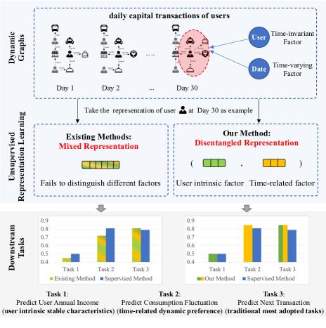
Figure 1. The effectiveness of the disentangled dynamic graphs representation in various downstream tasks. Note that, the existing method, supervised model, and our method share the same backbone model.

Existing methods for dynamic graph representation learning mainly fall into two categories (Sankar et al., 2020; Yang et al., 2021): continuous-time approaches and discrete-time approaches. The former regards new nodes or edges of dynamic graphs in a streaming manner and models the continuous temporal information via point process (Trivedi et al., 2019; Zuo et al., 2018) or temporal random walks (Yu et al., 2018; Nguyen et al., 2018b). This type of method usually requires finer-grained timestamps, which is however difficult to obtain in the real world for privacy protection. The latter regards the dynamic graphs as a series of snapshots changing at discrete time and adopts structure models (e.g., graph neural networks (Kipf and Welling, 2016; Velickovic et al., 2017)) to capture graph characteristics and temporal models (e.g., deep sequential neural networks (Bai et al., 2018; Vaswani et al., 2017)) to summarize historical information of each node (Pareja et al., 2020; Sankar et al., 2020; Yang et al., 2021), which is more practical.

Despite the preliminary success, existing methods typically adhere to a paradigm that generates a mixed representation for each node, neglecting to differentiate between the varying factors that determine dynamic graphs. As shown in Figure 1, taking the real dynamic graph of daily capital transactions on Tencent as an example, the daily transactions are determined by both the factor of user intrinsic characteristics and the factor of dates. Mixing these two kinds of factors into a single representation as existing methods leads to a limited ability when applied to various downstream tasks that require different types of information (bottom of Figure 1). In other words, there is still a lack of an effective dynamic graph representation learning method to handle various downstream tasks.

Recently, disentangled representation learning in various fields has demonstrated that separating the informative factors in representations is an essential step toward better representation learning (Locatello et al., 2019; Chen et al., 2021; Zhu et al., 2021). However, due to the non-Euclidean characteristics of graph structure and the complexity of temporal evolution, as well as the lack of guidance, how to learn disentangled dynamic graph representation still remains unexplored and challenging.

In this paper, we introduce a novel disenTangled representation learning framework for discrete-time Dynamic graphs, namely DyTed. Without loss of generality, we assume that the dynamic graph is a comprehensive embodiment of both the intrinsic stable characteristics of the node, referred to as the time-invariant factor, and the time-related dynamic preference, referred to as the time-varying factor. To effectively identify such two types of factors or information, we propose a time-invariant representation generator with the carefully designed temporal-clips contrastive learning task, together with a time-varying representation generator with structure contrastive learning. To further enhance the disentanglement or separation between time-invariant and time-varying representation, we propose a disentanglement-aware discriminator under an adversarial learning framework from the perspective of information theory. As shown in Figure 1, the different parts of disentangled representation perform well on downstream tasks, which is comparable to or even better than the supervised method.

Extensive experiments on Tencent and five commonly used public datasets demonstrate that our framework, as a general framework that can be applied to existing methods, significantly improves the performance of state-of-the-art methods on various downstream tasks including node classifications and link predictions. Also, we offer ablation studies to evaluate the importance of each part and conduct noise experiments to demonstrate the model’s robustness.

In summary, the main contributions are as follows:

• To the best of our knowledge, we are the first to study and introduce the disentangled representation learning framework for discrete-time dynamic graphs.

• We propose two representation generators with carefully designed pretext tasks and a disentanglement-aware discriminator under an adversarial learning framework.

• We conduct extensive experiments on real dynamic graphs of daily capital transactions on Tencent, achieving state-of-the-art performance on various downstream tasks.

2. RELATED WORK

This section briefly reviews the research on dynamic graph representation learning and disentangled representation learning.

2.1. Dynamic Graph Representation Learning

Representation learning for dynamic graphs aims to learn time-dependent low-dimensional representations of nodes (Xue et al., 2022), which can be mainly divided into continuous-time and discrete-time approaches according to the form of dynamic graphs. Continuous-time approaches treat the dynamic graphs as a flow of nodes or edges annotated with a specific timestamp (Nguyen et al., 2018a; Xu et al., 2020; Kumar et al., 2019). To incorporate the temporal information, either temporal random walks are sampled to serve as the context information of nodes (Nguyen et al., 2018b; Yu et al., 2018) or point process are adopted regarding the arrival of nodes/edges as an event (Chang et al., 2020; Trivedi et al., 2019; Zuo et al., 2018; Zhou et al., 2018). Although continuous-time approaches have demonstrated success, practical considerations such as privacy must be considered when collecting data in real-world scenarios, which makes it difficult to acquire fine-grained timestamps.

Another line of research regards the dynamic graphs as a series of snapshots (Sankar et al., 2020; Goyal et al., 2018; Pareja et al., 2020), which generally captures the characteristics of these snapshots via the structural and temporal models. Early methods adopt the matrix decomposition to capture the graph structure in each snapshot and regularize the smoothness of the representation of adjacent snapshots (Ahmed et al., 2018; Li et al., 2017). Unfortunately, such matrix decomposition is usually computationally complex (Xue et al., 2022). With the development of deep learning, graph neural networks (Kipf and Welling, 2016) are adopted to capture the structural information while recurrent neural networks or transformer (Vaswani et al., 2017) are further utilized to summarize the historical information (Wang et al., 2020; Pareja et al., 2020; Sankar et al., 2020). To effectively learn the representation, pretext tasks such as structure contrast (Sankar et al., 2020; Tian et al., 2021), graph reconstruction (Goyal et al., 2018; Cai et al., 2021), and link prediction (Yang et al., 2021) are further adopted to guide the model learning.

However, the above existing methods for dynamic graph representation learning generally mix various factors into a single representation, which makes it difficult to generalize the learned representation to different downstream tasks.

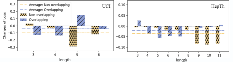
Figure 2. The average change proportion of overall loss after optimizing a certain type of positive pairs.

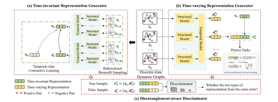
Figure 3. Overview of DyTed. (a) Time-invariant representation generator, composed of bidirectional Bernoulli sampling, structural-temporal modeling, and temporal-clips contrastive learning. (b) Time-varying representation generator, composed of structural-temporal modeling and pretext task in backbone models. (c) Disentanglement-aware discriminator, enhancing the separation between time-invariant and time-varying representation.

2.2. Disentangled Representation Learning

Recently, disentangled representation learning has attracted a lot of research attention and achieved great success in many fields (Chen et al., 2021; Ma et al., 2019; Locatello et al., 2019; Cao et al., 2022; Zhao et al., 2022; Wang et al., 2022). Specifically, in computer vision, the identity of a face is disentangled from the views or pose information to perform better on image recognition (Tran et al., 2017). In natural language generation, the writing style is disentangled from the text content to serve the text-style transfer tasks (John et al., 2019). In graph neural networks, the factor behind the formation of each edge is disentangled for semi-supervised node classification (Zhao et al., 2022). As demonstrated in existing research, the disentangling representation is an important step toward a better representation learning (Locatello et al., 2019), which is much closer to human perception and cognition as well as can be more robust, explainable, and transferrable.

However, due to the complexity of graph structure and temporal evolution, how to learn disentangled representation in dynamic graphs remains largely unexplored.

3. PROBLEM DEFINITION

In this paper, considering the availability of data, we focus on the discrete-time dynamic graph that is defined as a series of snapshots $\{\mathcal{G}^{1},\mathcal{G}^{2}…,\mathcal{G}^{T}\}$, where $T$ is the total number of snapshots. The snapshot at time $t$, i.e., $\mathcal{G}^{t}=(\mathcal{V}^{t},\mathcal{E}^{t})$, is a graph with a node set $\mathcal{V}^{t}$ and an edge set $\mathcal{E}^{t}\subseteq\mathcal{V}^{t}\times\mathcal{V}^{t}$. We use $\bm{A}^{t}$ to denote the adjacency matrix corresponding to the edge set $\mathcal{E}^{t}$. Note that, as time evolves, there may be both the appearance and disappearance of nodes or edges. Existing discrete-time dynamic graph representation learning aims to learn a low-dimensional representation $\bm{r}^{t}_{v}\in\mathbb{R}^{d}$ for each node $v\in\mathcal{V}^{t}$ at each timestamp $t$, which mix different types of information into a single representation space.

In this paper, we aim to disentangle the time-invariant and time-varying information in discrete-time dynamic graph representation learning, which is formally defined as follows:

Disentangled representation learning for discrete-time dynamic graphs Given a dynamic graph $\{\mathcal{G}^{1},\mathcal{G}^{2},...,\mathcal{G}^{T}\}$, for each node $v\in\mathcal{V}$, where $\mathcal{V}=\cup_{t=1}^{T}\mathcal{V}^{t}$, we aim to learn: (1) a time-invariant representation $\bm{s}_{v}\in\mathbb{R}^{\frac{d}{2}}$ that is independent of time and captures intrinsic stable characteristics of node $v$; (2) time-varying representations $\bm{d}_{v}^{t}\in\mathbb{R}^{\frac{d}{2}}$ at each timestamp $t$, that reflect the fluctuating preference of node $v$ related with time. The final disentangled representation $\bm{r}^{t}_{v}\in\mathbb{R}^{d}$ of node $v$ at timestamp $t$ is the combination of the above two types of representations: $\begin{aligned} \bm{r}_{v}^{t}=(\bm{s}_{v},\bm{d}_{v}^{t}).\end{aligned}$

In comparison to traditional representation learning methods, the disentangled representation learning approach separates the time-invariant and the time-varying information to address different downstream tasks. In addition, it’s worth noting that the total representation dimension of disentangled representation learning is comparable to or even less than traditional methods. Specifically, as the time-invariant representation is consistent across all snapshots, the resulting representation in disentangle representation learning is $\bm{r}_{v}=(\bm{s}_{v},\bm{d}_{v}^{1,...,T})\in\mathbb{R}^{(T+1)\times\frac{d}{2}}$, whereas the representation obtained using traditional methods is $\bm{r}_{v}=(\bm{r}_{v}^{1,...,T})\in\mathbb{R}^{T\times d}$.

4. Method

In this section, we present a disentangled representation learning framework for discrete-time dynamic graphs, namely DyTed. To effectively identify the two types of information in dynamic graphs, i.e., time-invariant and time-varying factors, we propose two representation generators and a disentanglement-aware discriminator under an adversarial learning framework. The overview of the framework is shown in Figure 3, where the backbone model in the blue box can be replaced with any existing discrete-time dynamic graph representation learning method. Next, we introduce each part in detail.

4.1. Time-invariant Representation Learning

The time-invariant representation generator aims to identify the intrinsic stable characteristics of nodes, which is not easy to learn due to the lack of explicit guidance information. To address this challenge, we consider the fundamental nature behind the time-invariant representation, that is, such properties of nodes should be identified as the same in any local temporal clips. Based on this understanding, we design an effective temporal-clips contrastive learning as the pretext task, together with a bidirectional Bernoulli sampling and structural-temporal modeling module.

4.1.1. Observation

We first define the temporal clips as a part of successive snapshots. In order to achieve the above objective for time-invariant representation of node $v$, the most straightforward way is to sample all pairs of two temporal clips and optimize the representations of node $v$ in any pair to be the same. However, such a way may result in a total of $\mathcal{O}(T^{4})$ pairs where $T$ is the number of snapshots, which is too large to lead to a low optimization efficiency. To solve this challenge, we aim to minimize the objective by finding some cost-effective pairs. Through experiments, as shown in Figure 2, we have three interesting observations: 1). On average, optimizing non-overlapping pairs benefits more for the overall loss reduction than overlapping pairs, i.e., the yellow dotted line is lower than the blue dotted line. 2). For non-overlapping pairs, optimizing long pairs, i.e. pairs with long temporal clips, are more effective than short pairs. 3). For overlapping pairs, the result is reverse, that is, optimizing short pairs are more effective. For more details, please refer to Appendix A.1.

4.1.2. Bidirectional Bernoulli sampling

Based on the above observed three rules, we design the bidirectional Bernoulli sampling to higher the sampling probability of more cost-effective pairs of temporal clips.

Definition 4.1.

Truncated geometric distribution. Let $p\in(0,1)$ be the probability of success on each Bernoulli trial, $m\in\mathbb{N}^{+}$ be the number of Bernoulli trials when we get the first success. Given $m\in[1,L]$, it follows the truncated geometric distribution as follows:

(1) $$Geo(p,L)\sim f(m;p;L)=p(1-p)^{(m-1)}\Phi(L)^{-1},$$

where $\Phi(L)=\sum^{L}_{m=1}p(1-p)^{(m-1)}$. We have $\mathbb{E}(m)=\frac{1}{p}-\frac{L(1-p)^{L}}{1-(1-p)^{L}}$.

Definition 4.2.

Bidirectional Bernoulli sampling. Let $t_{i}\in\mathbb{N}^{+}$ be the start timestamp for the first temporal clips and $t_{j}\in\mathbb{N}^{+}$ be the end timestamp for the second temporal clips. Let $L=t_{j}-t_{i}+1$ denote the clips range from $t_{i}$ to $t_{j}$. We sample $L$ from uniform distribution $U(1,T)$ and $t_{i}$ from $U(1,T-L)$, where $T$ is the total number of snapshots. Then the length of the two temporal clips $m_{1},m_{2}\in\mathbb{N}$ is drawn i.i.d. from truncated geometric distribution $Geo(p=\psi(L),L)$, where $\psi(L)$ is a decreasing function related to $L$. Following the above sampling process, two temporal clips are sampled as:

(2) $$\mathcal{C}_{1} =[\mathcal{G}^{t_{i}},\mathcal{G}^{t_{i}+1},...,\mathcal{G}^{t_{i}+m_{1}-1}],$$

$$\mathcal{C}_{2} =[\mathcal{G}^{t_{j}-m_{2}+1},\mathcal{G}^{t_{j}-m_{2}+2},...,\mathcal{G}^{t_{j}}].$$

Next, we analyze whether the pair of temporal clips $\mathcal{C}_{1},\mathcal{C}_{2}$ sampled via the above Bidirectional Bernoulli sampling can satisfy the observed three rules.

Proposition 4.1.

Let pairs of two temporal clips $\mathcal{C}_{1},\mathcal{C}_{2}$ be sampled from bidirectional Bernoulli sampling. Let $X=1$ denote that $\mathcal{C}_{1}$ and $\mathcal{C}_{2}$ have overlapped snapshots, otherwise $X=0$. When probability $p=\psi(L)$ in truncated geometric distribution satisfies that $\frac{2}{L+2}\leq p<1$ and $L\geq 3$, then we have:

(3) $$\frac{Pr(X=1)}{Pr(X=0)}\leq 1,\frac{Pr(L=l+1|X=0)}{Pr(L=l|X=0)}\geq 1,\frac{Pr(L=l+1|X=1)}{Pr(L=l|X=1)}\leq 1.$$

$Proof.$ see Appendix A.2. In Proposition 3, $\frac{Pr(X=1)}{Pr(X=0)}\leq 1$ indicates that the sampled probability of non-overlapping pairs is higher than overlapping pairs, satisfying the observation 1). $\frac{Pr(L=l+1|X=0)}{Pr(L=l|X=0)}\geq 1$ indicates that for non-overlapping pairs, the sampled clips range $L$ is more like to be large. Recall that $p=\psi(L)$ is a decreasing function related to $L$, i.e., $\psi(L)^{\prime}\leq 0$, then we can easily obtain that $\nabla_{L}\mathbb{E}_{G(p=\psi(L),L)}(m)\geq 0$. In other words, the larger the sampled clips gap $L$, the longer the expected length of the sampled temporal clips $\mathbb{E}(m)$ is, satisfying observation 2). Similarly, $\frac{Pr(L=l+1|X=1)}{Pr(L=l|X=1)}\leq 1$ indicates the satisfaction of observation 3).

To sum up, as long as $\frac{2}{L+2}\leq p=\psi(L)<1$, $\psi(L)^{\prime}\leq 0$, and $L\geq 3$, we have demonstrated that the proposed Bidirectional Bernoulli sampling has the ability to sample the cost-effective pairs of temporal clips with higher probability. In this paper, we design an exampled implementation of $\psi(L)$ to satisfy these constraints, i.e., $\psi(L)=1-\alpha\frac{L}{L+2}$, where the $0<\alpha\leq 1$ is a learnable parameter.

4.1.3. Temporal-clips Contrastive Learning

With the development of deep neural networks, the state-of-the-art methods for discrete-time dynamic graph representation learning generally follow a structural-temporal paradigm (Sankar et al., 2020; Yang et al., 2021). Here, we also take such structural-temporal models to generate the representation. Specifically, given two sampled temporal clips $\mathcal{C}_{1}$ and $\mathcal{C}_{2}$, the representation of time-invariant generator for node $v$ is denoted as:

(4) $$\bm{s}^{1}_{v}={G_{i}}(\mathcal{C}_{1})_{v},\bm{s}^{2}_{v}={G_{i}}(\mathcal{C}_{2})_{v},$$

where $G_{i}$ can be any backbone model in existing methods.

To optimize the time-invariant generator $G_{i}$, we take the representation of node $v$ for two temporal clips sampled via Bidirectional Bernoulli sampling as the positive pair in contrastive learning, i.e., $(\bm{s}_{v}^{1},\bm{s}_{v}^{2})$, and take the representation of node $v$ for $\mathcal{C}_{1}$ and the representation of node $u$ for $\mathcal{C}_{1}$ as the negative pair, i.e., $(\bm{s}_{v}^{1},\bm{s}_{u}^{1})$. We use InfoNCE (Oord et al., 2018) as the contrastive loss to separate the positive pair and the negative pairs. Such contrastive loss can maximize the mutual information between representations in positive pairs while minimizing the mutual information between representations in negative pairs, ensuring that the extracted representations of the same node in different temporal clips are similar. The loss function is formalized as follows:

(5) $$L_{i}(G_{i})=\mathbb{E}_{v}\left[-\log\left(\frac{\exp\left({\rm sim}(\bm{s}_{v}^{1},{\bm{s}_{v}^{2}})/\tau\right)}{\sum_{u\in\mathcal{V}}\exp\left({\rm sim}(\bm{s}_{v}^{1},{\bm{s}_{u}^{1}})/\tau\right)}\right)\right],$$

where $\rm sim(\cdot)$ is the similarity function, and $\tau$ is the temperature.

Note that, the final time-invariant representation $\bm{s}_{v}$ for node $v$ is obtained when the temporal clip contains all snapshots, i.e., $\bm{s}_{v}={G_{i}}([\mathcal{G}^{1},\mathcal{G}^{2},...,\mathcal{G}^{T}])_{v}$.

4.2. Time-varying Representation Learning

For the time-varying representation generator, we use the same backbone model as the time-invariant generator with non-shared parameters. The time-varying representation for node $v$ at timestamp $t$ is denoted as $\bm{d}_{v}^{t}$:

(6) $$={G_{v}}\left([\mathcal{G}^{1},\mathcal{G}^{2},...,\mathcal{G}^{T}]\right)_{v}.$$

Considering that the graph structure and the evaluation are the comprehensive embodiment of both the time-invariant and time-varying representations, we combine the time-invariant representation $\bm{s}_{v}$ and time-varying representation $\bm{d}_{v}^{t}$ together, i.e., $\bm{r}_{v}^{t}=(\bm{s}_{v},\bm{d}_{v}^{t})$, to complete the self-supervise task related to the evolution characteristics of dynamic graphs. Worth noting, the self-supervise task can be the same as the tasks in the backbone model or other well-design self-supervising tasks, such as structure-proximity contrastive learning:

(7) $$L_{v}(G=\{G_{i},G_{v}\})=\sum_{t=1}^{T}\mathbb{E}_{(u,v)\in\mathcal{E}_{t}}\left[-\log\left(\frac{\exp\left({\rm sim}(r_{v}^{t},r_{u}^{t})/\tau\right)}{\sum_{w\in\mathcal{U}}\exp\left({\rm sim}(r_{v}^{t},r_{w}^{t})/\tau\right)}\right)\right].$$

or link prediction:

(8) $$L_{v}(G)=-\sum_{t=1}^{T-1}\left[\mathbb{E}_{(u,v)\in\mathcal{E}_{t+1}}\log\left(r_{v}^{t\top}r_{u}^{t}\right)+\mathbb{E}_{(u,w)\notin\mathcal{E}_{t+1}}\log\left(1-(r_{v}^{t\top}r_{w}^{t})\right)\right].$$

4.3. Disentanglement-aware Discriminator

Algorithm 1 The training procedure of DyTed

1:Dynamic graph $[\mathcal{G}^{1},\mathcal{G}^{2},...,\mathcal{G}^{T}]$

2:Time-invariant representations $\bm{S}\in\mathbb{R}^{N\times\frac{d}{2}}$; Time-varying representations $\bm{D}^{t}\in\mathbb{R}^{N\times\frac{d}{2}}$, $t=1,...,T$.

3:while not Convergence do

4:    Draw $L$ from $U(1,T)$ and $t_{i}$ from $U(1,T-L)$, calculate $t_{j}=t_{i}+L-1$.

5:    Calculate the sampling vectors $\bm{k}^{1},\bm{k}^{2}$ according to Eq. 13

6:    Calculate the snapshots index vector $\bm{k}^{i}=\{k^{i}_{j}=k^{i}_{j}+k^{i}_{j+1}\}_{j=L-1}^{1}$, $i=1,2$

7:    $\mathcal{C}_{1}=[\mathcal{G}^{m}\cdot k^{1}_{m-t_{i}}]_{m=t_{i}}^{t_{j}}$, $\mathcal{C}_{2}=[\mathcal{G}^{m}\cdot k^{2}_{t_{j}-m}]_{m=t_{i}}^{t_{j}}$

8:    Time-invariant representations: $\bm{S}^{1}=G_{i}(\mathcal{C}_{1})$, $\bm{S}^{2}=G_{i}(\mathcal{C}_{2})$

9:    Time-varying representations: $[\bm{D}^{1},\bm{D}^{2},...,\bm{D}^{T}]={G_{v}}([\mathcal{G}^{i}]_{i=1}^{T})$

10:    Calculate $Loss(G)$ according to Eq. 12 and minimize $Loss(G)$

11:    for Epochs of Discriminator do

12:         Calculate $Loss(D)$ according to Eq. 10 and minimize $Loss(D)$

13:    end for

14:end while

15:Final time-invariant representation: $\bm{S}=G_{i}([\mathcal{G}^{i}]_{i=1}^{T}$)

16:return $\bm{S}$, $[\bm{D}^{1},\bm{D}^{2},...,\bm{D}^{T}]$

After the time-invariant and the time-varying representation generator, we get two parts of representations. To further enhance the disentanglement between these two types of information, we propose an adversarial learning framework from the perspective of information theory.

Imagine that if the time-invariant representations $\bm{s_{v}}\in\mathbb{R}^{\frac{d}{2}}$ and the time-varying representations $\bm{d^{t}_{v}}\in\mathbb{R}^{\frac{d}{2}}$ are not well disentangled, i.e., there is some overlap in the information of the representations. From the perspective of information theory, this overlap can be quantified using the mutual information $I(\bm{S},\bm{D})$, where $\bm{S}$ is the distribution of time-invariant representations for all nodes and $\bm{D}$ is the distribution of time-varying representations for all nodes. In other words, to enhance the disentanglement between the time-invariant and time-varying representations, we aim to minimize the mutual information between them, i.e.,

(9) $$\min_{G=\{G_{i},G_{v}\}}I(\bm{S},\bm{D}),$$

Considering that $I(\bm{S},\bm{D})=\sum_{s\in\bm{S}}\sum_{d\in\bm{D}}p(s,d)\log\frac{p(s,d)}{p(s)p(d)}=\mathcal{D}_{kl}(p(\bm{S},\bm{D})||p(\bm{S})p(\bm{D}))$, minimizing the mutual information is equivalent to minimizing the KL divergence between distribution $p(\bm{S},\bm{D})$ and $p(\bm{S})p(\bm{D})$. As a result, we construct the true data distribution as $p_{d}=p(\bm{S},\bm{D})$ and the generated data distribution as $p_{g}=p(\bm{S})p(\bm{D})$, and introduce the framework of generative adversarial networks to minimize the KL divergence between these two data distributions, i.e.,

(10) $$\min_{G}\max_{D}V(G,D)=\min_{G}\max_{D}\mathbb{E}_{T}\left(\log\left(D\left(\bm{r}_{i}^{t}\right)\right)+\log\left(1-D\left(\bm{z}_{i}^{t}\right)\right)\right)$$

where $\bm{r}_{i}^{t}=(\bm{s}_{v},\bm{d}_{v}^{t})$ is the true sample that randomly sampled from the same node, $\bm{z}_{i}^{t}=(\bm{s}_{v},\bm{d}_{u}^{t})$ is the false sample that randomly sampled from two nodes. $D$ is the disentanglement-aware discriminator implemented by multi-layer perceptron (MLP), which can distinguish whether the time-invariant and the time-varying representation come from the same node, telling generators if two parts representations have overlapped information.

Finally, the loss function of the discriminator is:

(11) $$Loss(D)=-V(G,D)$$

and the loss function of the generators is:

(12) $$Loss(G=\{G_{i},G_{v}\})=L_{v}(G)+\lambda_{1}L_{i}(G_{i})+\lambda_{2}V(G,D)+\lambda_{3}||w||_{2}^{2}$$

where $\lambda_{1},\lambda_{2}$ and $\lambda_{3}$ are hyperparameters.

4.4. Training Strategy

In order to train the parameters of bidirectional Bernoulli sampling, we introduce the categorical reparameterization (Jang et al., 2016). Given the truncated geometric distribution $Geo(p,L)$ and the probabilities of sampling length $m=1,2,...,L$ for temporal clips as $p_{m}=f(m;p;L)$, then we can generate $L$-dimensional sampling vectors $\bm{k}\in\mathbb{R}^{l}$:

(13) $$k_{m}=\frac{\exp\left(\left(\log(p_{m})+g_{m}\right)/\tau_{g}\right)}{\sum_{j=1}^{L}\exp\left(\left(\log(p_{j})+g_{j}\right)/\tau_{g}\right)},~{}~{}~{}~{}\rm{for}~{}m=1,2,...,L.$$

where $g_{m}$ is i.i.d. drawn from Gumbel distribution $\rm{Gumbel}(0,1)$ and $\tau_{g}$ is the temperature parameter.

Finally, we can propagate the gradient to parameter $\alpha$ in bidirectional Bernoulli sampling by sampling vectors $\bm{k}$. The procedure of training DyTed is illustrated in Algorithm 1.

4.5. Complexity Analysis

Without loss of generality, we assume that the time complexity of the backbone model is $\mathcal{O}(M)$. Then, when we further attach our framework to the backbone model, the time complexity is $\mathcal{O}(\frac{3}{2}M+n|\mathcal{V}|d+n^{\prime}d)$, where $\frac{3}{2}$ is due to three calculations of $\mathcal{C}_{1}$, $\mathcal{C}_{2}$ in the time-invariant generator and the entire dynamic graph in the time-varying generator, as well as the half dimension of representation in DyTed. $\mathcal{O}(n|\mathcal{V}|d)$ is the time complexity of the temporal-clips contrastive learning, where $n$ is the number of negative pairs for each positive pair in InfoNCE, and $d$ is the dimension of representations. $\mathcal{O}(n^{\prime}d)$ is the time complexity of the discriminator, where $n^{\prime}$ is the number of ture and false samples. In general, $\mathcal{O}(\mathcal{M})\gg\mathcal{O}(n|\mathcal{V}|d+n^{\prime}d)$. For example, when the backbone model is a simple GCN plus LSTM, $\mathcal{O}(M)=\mathcal{O}(T|\mathcal{E}||\mathcal{V}|d)\gg\mathcal{O}(n|\mathcal{V}|d+n^{\prime}d)$. As a result, compared with the backbone model, the time complexity of DyTed does not increase in magnitude. See Figure 8 in Appendix A.3 for more experimental results.

5. EXPERIMENTS

Table 1. Datasets

DATASET	#Nodes	#Edges	#Snapshots
UCI	1,809	56,459	13
Bitcoin	3,782	483,700	20
AS733	4,648	532,230	30
HepTh	7,576	196,463	23
HepPh	10,404	339,556	20
Tencent-alpha	11,623	102,464	30
Tencent-beta	115,190	6,680,276	30

In this section, we conduct extensive experiments to answer the following research questions (RQs). Due to space limitations, some experimental results or details are in Appendix.

• RQ1: Whether the DyTed framework can improve the performance of existing methods in various downstream tasks?

• RQ2. What does each component of DyTed bring?

• RQ3: Is there any additional benefit of disentanglement?

5.1. Experimental Setup

Table 2. Node classification for Tencent-alpha

Model	Annual Income		Age		Assets		Financing Risk		Consumption Fluctuation
	micro-F1	macro-F1	micro-F1	macro-F1	micro-F1	macro-F1	micro-F1	macro-F1	micro-F1	macro-F1
LSTMGCN	50.38 $\pm$ 0.38	27.12 $\pm$ 0.32	34.86 $\pm$ 0.48	17.98 $\pm$ 1.08	24.06 $\pm$ 0.46	16.37 $\pm$ 0.39	49.13 $\pm$ 0.32	29.56 $\pm$ 0.64	93.70 $\pm$ 0.06	93.65 $\pm$ 0.06
LSTMGCN-DyTed	(+7.23% $\uparrow$)	(+10.55% $\uparrow$)	(+1.55% $\uparrow$)	(+23.30% $\uparrow$)	(+6.77% $\uparrow$)	(+20.95% $\uparrow$)	(+2.89% $\uparrow$)	(+6.76% $\uparrow$)	(+3.18% $\uparrow$)	(+2.36% $\uparrow$)
-Combine	51.14 $\pm$ 0.46	28.21 $\pm$ 0.49	33.64 $\pm$ 0.56	21.13 $\pm$ 0.43	25.51 $\pm$ 0.54	19.14 $\pm$ 0.55	48.29 $\pm$ 0.55	31.56 $\pm$ 0.21	95.91 $\pm$ 0.33	95.83 $\pm$ 0.32
-Time-invariant	54.02 $\pm$ 0.35	29.98 $\pm$ 0.72	35.40 $\pm$ 0.20	22.17 $\pm$ 0.21	25.69 $\pm$ 0.26	19.80 $\pm$ 0.41	50.55 $\pm$ 0.50	31.42 $\pm$ 0.98	74.05 $\pm$ 0.99	73.32 $\pm$ 1.02
-Time-varying	52.45 $\pm$ 0.18	23.82 $\pm$ 0.21	34.04 $\pm$ 0.55	15.12 $\pm$ 0.47	25.39 $\pm$ 0.18	15.02 $\pm$ 0.31	49.03 $\pm$ 0.35	24.98 $\pm$ 1.09	96.68 $\pm$ 0.21	95.86 $\pm$ 0.20
DySAT	46.65 $\pm$ 3.12	25.34 $\pm$ 0.97	28.92 $\pm$ 3.18	13.54 $\pm$ 1.28	25.50 $\pm$ 0.58	13.06 $\pm$ 0.46	42.95 $\pm$ 2.46	25.03 $\pm$ 0.74	72.73 $\pm$ 2.06	71.21 $\pm$ 2.18
DySAT-DyTed	(+13.48$\%$ $\uparrow$)	(+10.22$\%$ $\uparrow$)	(+15.08$\%$ $\uparrow$)	(+38.63$\%$ $\uparrow$)	(+9.73$\%$ $\uparrow$)	(+26.26$\%$ $\uparrow$)	(+15.32$\%$ $\uparrow$)	(+14.74$\%$ $\uparrow$)	(+16.72$\%$ $\uparrow$)	(+19.15$\%$ $\uparrow$)
-Combine	49.39 $\pm$ 3.31	27.82 $\pm$ 1.76	28.07 $\pm$ 4.55	13.93 $\pm$ 2.04	25.88 $\pm$ 0.52	13.12 $\pm$ 0.62	45.66 $\pm$ 4.65	33.13 $\pm$ 3.09	80.11 $\pm$ 1.96	79.98 $\pm$ 2.05
-Time-invariant	52.94 $\pm$ 0.48	27.93 $\pm$ 0.50	33.28 $\pm$ 0.73	18.77 $\pm$ 0.94	27.98 $\pm$ 0.71	16.49 $\pm$ 0.82	49.53 $\pm$ 0.42	28.72 $\pm$ 1.32	71.48 $\pm$ 2.05	71.11 $\pm$ 2.07
-Time-varying	40.41 $\pm$ 4.87	25.16 $\pm$ 1.96	23.87 $\pm$ 1.42	11.74 $\pm$ 1.08	23.06 $\pm$ 1.22	11.25 $\pm$ 0.87	42.01 $\pm$ 3.10	26.05 $\pm$ 0.88	84.89 $\pm$ 1.66	84.85 $\pm$ 1.66
EvolveGCN	48.26 $\pm$ 1.01	23.89 $\pm$ 1.07	31.02 $\pm$ 0.88	12.64 $\pm$ 0.74	24.39 $\pm$ 1.02	11.62 $\pm$ 0.17	43.76 $\pm$ 1.00	25.76 $\pm$ 0.40	92.00 $\pm$ 0.39	92.14 $\pm$ 0.39
EvolveGCN-DyTed	(+11.33$\%$ $\uparrow$)	(+3.47$\%$ $\uparrow$)	(+15.73$\%$ $\uparrow$)	(+19.86$\%$ $\uparrow$)	(+11.19$\%$ $\uparrow$)	(+30.12$\%$ $\uparrow$)	(+15.68$\%$ $\uparrow$)	(+1.28$\%$ $\uparrow$)	(+4.62$\%$ $\uparrow$)	(+5.18$\%$ $\uparrow$)
-Combine	53.00 $\pm$ 0.84	24.72 $\pm$ 1.19	35.06 $\pm$ 0.64	13.43 $\pm$ 0.54	26.86 $\pm$ 0.35	12.39 $\pm$ 0.18	47.96 $\pm$ 1.50	26.08 $\pm$ 0.29	96.25 $\pm$ 0.08	96.20 $\pm$ 0.06
-Time-invariant	53.73 $\pm$ 0.40	23.38 $\pm$ 0.08	35.90 $\pm$ 0.31	15.15 $\pm$ 0.45	27.12 $\pm$ 0.30	15.12 $\pm$ 0.64	50.62 $\pm$ 0.58	26.09 $\pm$ 0.92	76.45 $\pm$ 2.11	79.71 $\pm$ 2.11
-Time-varying	52.53 $\pm$ 1.03	24.63 $\pm$ 1.12	34.78 $\pm$ 0.58	12.11 $\pm$ 0.61	26.37 $\pm$ 0.89	10.87 $\pm$ 0.17	47.82 $\pm$ 1.65	24.05 $\pm$ 0.55	96.02 $\pm$ 0.08	96.91 $\pm$ 0.08
HTGN	54.11 $\pm$ 0.46	23.41 $\pm$ 0.13	35.74 $\pm$ 0.36	10.53 $\pm$ 0.08	26.70 $\pm$ 0.39	11.25 $\pm$ 0.71	50.13 $\pm$ 0.19	22.26 $\pm$ 0.06	92.25 $\pm$ 1.54	92.14 $\pm$ 1.57
HTGN-DyTed	(+1.81$\%$ $\uparrow$)	(+1.11$\%$ $\uparrow$)	(+3.47$\%$ $\uparrow$)	(+9.78$\%$ $\uparrow$)	(+6.55$\%$ $\uparrow$)	(+29.69$\%$ $\uparrow$)	(+3.97$\%$ $\uparrow$)	(+4.49$\%$ $\uparrow$)	(+4.80$\%$ $\uparrow$)	(+4.87$\%$ $\uparrow$)
-Combine	53.26 $\pm$ 0.55	23.17 $\pm$ 0.16	36.50 $\pm$ 0.39	10.50 $\pm$ 0.08	27.43 $\pm$ 0.38	12.96 $\pm$ 0.77	49.86 $\pm$ 0.36	22.18 $\pm$ 0.11	96.57 $\pm$ 0.09	96.52 $\pm$ 0.09
-Time-invariant	55.09 $\pm$ 0.46	23.67 $\pm$ 0.13	36.98 $\pm$ 0.34	11.56 $\pm$ 0.07	28.45 $\pm$ 0.29	14.59 $\pm$ 0.07	52.12 $\pm$ 0.25	23.26 $\pm$ 0.08	93.30 $\pm$ 0.29	93.21 $\pm$ 0.29
-Time-varying	53.06 $\pm$ 0.37	23.11 $\pm$ 0.10	35.66 $\pm$ 0.46	10.51 $\pm$ 0.10	26.99 $\pm$ 0.37	8.97 $\pm$ 0.21	49.08 $\pm$ 0.30	21.95 $\pm$ 0.09	96.68 $\pm$ 0.11	96.63 $\pm$ 0.12
ROLAND	50.62 $\pm$ 0.40	20.27 $\pm$ 0.11	31.21 $\pm$ 0.34	10.41 $\pm$ 0.08	28.08 $\pm$ 0.43	8.77 $\pm$ 0.10	49.34 $\pm$ 0.42	22.02 $\pm$ 0.12	83.27 $\pm$ 0.16	75.18 $\pm$ 0.07
ROLAND-DyTed	(+9.40$\%$ $\uparrow$)	(+24.32$\%$ $\uparrow$)	(+15.54$\%$ $\uparrow$)	(+20.94$\%$ $\uparrow$)	(+3.74$\%$ $\uparrow$)	(+11.97$\%$ $\uparrow$)	(+5.78$\%$ $\uparrow$)	(+11.58$\%$ $\uparrow$)	(+8.47$\%$ $\uparrow$)	(+7.37$\%$ $\uparrow$)
-Combine	54.01 $\pm$ 0.51	23.38 $\pm$ 0.14	36.04 $\pm$ 0.23	11.60 $\pm$ 0.05	28.50 $\pm$ 0.32	8.87 $\pm$ 0.08	50.11 $\pm$ 0.24	22.25 $\pm$ 0.07	85.45 $\pm$ 0.21	75.67 $\pm$ 0.09
-Time-invariant	55.38 $\pm$ 0.36	25.20 $\pm$ 0.10	36.06 $\pm$ 0.47	12.59 $\pm$ 0.10	29.13 $\pm$ 0.37	9.82 $\pm$ 0.17	52.19 $\pm$ 0.36	24.57 $\pm$ 0.11	84.25 $\pm$ 0.20	75.17 $\pm$ 0.09
-Time-varying	53.76 $\pm$ 0.32	23.01 $\pm$ 0.09	35.13 $\pm$ 0.34	10.40 $\pm$ 0.08	27.63 $\pm$ 0.47	8.67 $\pm$ 0.12	49.15 $\pm$ 0.46	21.97 $\pm$ 0.14	90.32 $\pm$ 0.27	80.72 $\pm$ 0.12

In this section, we introduce the details of experimental setup.

5.1.1. Datasets

In order to evaluate our proposed method, we adopt five commonly used datasets of dynamic graphs, including the communication network UCI (Panzarasa et al., 2009), bitcoin transaction network Bitcoin (Kumar et al., 2018), routing network AS733 (Leskovec et al., 2005), citation network HepTh and HepPh (Leskovec et al., 2005). In addition, we also include two real financial datasets of dynamic graphs, Tecent-alpha and Tencent-beta, with high-quality user labels and various downstream tasks. The detailed statistics of all datasets are shown in Table 1.

• UCI (Panzarasa et al., 2009) is a communication network, where links represent messages sent between users on an online social network.

• Bitcoin (Kumar et al., 2018) is a who-trusts-whom network of people who trade using Bitcoin.

• AS733 (Leskovec et al., 2005) is a routing network. The dataset contains a total of 733 snapshots. We follow the setting in (Yang et al., 2021) and extract 30 snapshots. To enable all baselines to conduct experiments, we restricted the dataset not to include deleted nodes.

• HepTh (Leskovec et al., 2005) is a citation network related to high-energy physics theory. We extract 92 months of data from this dataset, forming 23 snapshots. For each reference edge, we set it to exist since the occurrence of the reference.

• HepPh (Leskovec et al., 2005) is a citation network related to high-energy physics phenomenology. We extract 60 months of data from this dataset, forming 20 snapshots. Other settings are similar to HepTh.

• Tencent-alpha is real dynamic graphs of daily capital transactions between users on Tencent after eliminating sensitive information. Each node represents a customer or a business, and each edge represents the transaction. The data ranges from April 1, 2020, to April 30, 2020, with 30 snapshots. Each node has five labels that reflect the time-invariant or time-varying characteristics of users, i.e., annual income grade with five classes, age with five classes, asset with five classes, financing risk with three classes, and consumption fluctuation, i.e. the increase or decrease in daily consumption of users, with binary class.

• Tencent-beta has the same data source as Tencent-alpha, but Tencent-beta has more nodes with only two labels, i.e. asset with five classes and financing risk with five classes.

5.1.2. Baselines

We apply the proposed framework DyTed to the following five baselines. First, we select the combination of GCN (Kipf and Welling, 2016) and LSTM (denoted as LSTMGCN) as a basic baseline. Then we choose three state-of-the-art discrete-time approaches with contrastive or prediction pretext task, i.e., DySAT (Sankar et al., 2020) with the contrastive task, EvolveGCN (Pareja et al., 2020) and HTGN (Yang et al., 2021) with the predictive task. In addition, we choose a framework ROLAND (You et al., 2022) that extends the static model to the discrete-time dynamic graph representation learning. Note that, all the baselines learn representations in a single mixed space.

• DySAT (Sankar et al., 2020) computes node representations through joint self-attention along the two dimensions of the structural neighborhood and temporal dynamics.

• EvolveGCN (Pareja et al., 2020) adapts the GCN to compute node representations, and captures the dynamism of the graph sequence by using an RNN to evolve the GCN parameters.

• HTGN (Yang et al., 2021) maps the dynamic graph into hyperbolic space, and incorporates hyperbolic graph neural network and hyperbolic gated recurrent neural network to obtain representations.

• ROLAND (You et al., 2022) views the node representations at different GNN layers as hierarchical node states and recurrently updates them.

5.1.3. Implementation Details

For all baselines and our DyTed, the representation model is trained on the snapshots $\{\mathcal{G}^{1},\mathcal{G}^{2},...,\mathcal{G}^{T}\}$. The total dimension of the representation is set according to the scale of datasets, chosen from $\{16,32,64,128\}$. We ensure that the dimensions of the representation of each method are equal on the same dataset. We follow the hyperparameters given in the paper of the baselines. The stop of the training process depends on the loss of the pretext task. The learning rate is chosen from $\{0.1,0.01,...,10^{-5}\}$. In our framework, we choose $\lambda_{1}$ and $\lambda_{2}$ from $\{0.1,0.2,...,1.0\}$, and set $\lambda_{3}$ to $5e-7$, temperature parameter $\tau$ to $0.1$ and $\tau_{g}$ to $0.01$. ${\rm sim}(\cdot)$ mentioned in Section 4 is a cosine function. Our implementation code is provided through the link .

5.2. Performance on Downstream Tasks

In this section, we answer RQ1, i.e., whether the DyTed framework can improve the performance of existing methods in various downstream tasks? We evaluate the performance of our method using three diverse tasks: node classification with time-invariant labels, node classification with the time-varying label, and link prediction for the next snapshot. For clarity, we use some abbreviations to denote the different representations as follows:

• Baseline: the representations from the original baselines, , i.e., $\bm{r}_{v}^{t}\in\mathbb{R}^{d},t=1,2,...,T$ for node $v$.

• Baseline-DyTed: apply the proposed DyTed framework to the baseline method.

• -Combine: the combination of time-invariant and time-varying representation, i.e., $\bm{r}_{v}^{t}=(\bm{s}_{v},\bm{d}_{v}^{t})\in\mathbb{R}^{d},t=1,2,...,T$ for node $v$.

• -Time-invariant: only the time-invariant representation $\bm{s}_{v}\in\mathbb{R}^{\frac{d}{2}}$ for node $v$.

• -Time-varying: only the time-varying representation $\bm{d}_{v}^{t}\in\mathbb{R}^{\frac{d}{2}},t=1,2,...,T$ for node $v$.

Table 3. Node classification on Tencent-beta

Model	Assets		Finacing Risk
	micro-F1	macro-F1	micro-F1	macro-F1
LSTMGCN	33.03 $\pm$ 0.51	18.95 $\pm$ 0.87	29.59 $\pm$ 0.52	19.25 $\pm$ 0.52
LSTMGCN-DyTed	(+11.96% $\uparrow$)	(+6.39% $\uparrow$)	(+9.33% $\uparrow$)	(+10.81% $\uparrow$)
-Combine	36.61 $\pm$ 0.45	20.08 $\pm$ 0.41	30.64 $\pm$ 0.60	20.10 $\pm$ 0.29
-Time-invariant	36.98 $\pm$ 0.30	20.16 $\pm$ 0.22	32.35 $\pm$ 0.41	21.33 $\pm$ 0.43
-Time-varying	34.65 $\pm$ 0.40	16.78 $\pm$ 0.59	30.36 $\pm$ 0.37	19.43 $\pm$ 0.48
DySAT	OOM 1	OOM	OOM	OOM
EvolveGCN	39.21 $\pm$ 0.40	22.17 $\pm$ 0.46	37.56 $\pm$ 0.70	22.16 $\pm$ 1.33
EvolveGCN-DyTed	(+5.43% $\uparrow$)	(+12.00% $\uparrow$)	(+1.54% $\uparrow$)	(+14.89% $\uparrow$)
-Combine	41.34 $\pm$ 0.76	24.38 $\pm$ 0.47	37.78 $\pm$ 0.71	25.19 $\pm$ 0.31
-Time-invariant	40.78 $\pm$ 0.46	24.83 $\pm$ 0.29	38.14 $\pm$ 0.72	25.46 $\pm$ 0.29
-Time-varying	39.07 $\pm$ 0.37	21.63 $\pm$ 0.31	37.01 $\pm$ 0.43	25.03 $\pm$ 0.67
HTGN	OOM	OOM	OOM	OOM
ROLAND	33.59 $\pm$ 0.15	10.06 $\pm$ 0.04	33.05 $\pm$ 0.37	9.93 $\pm$ 0.08
ROLAND-DyTed	(+10.87% $\uparrow$)	(+103.38% $\uparrow$)	(+6.20% $\uparrow$)	(+63.44% $\uparrow$)
-Combine	36.01 $\pm$ 0.65	19.11 $\pm$ 0.56	34.47 $\pm$ 0.74	15.61 $\pm$ 0.83
-Time-invariant	37.24 $\pm$ 1.01	20.46 $\pm$ 0.21	35.10 $\pm$ 0.47	16.23 $\pm$ 0.81
-Time-varying	33.23 $\pm$ 0.31	9.98 $\pm$ 0.07	33.24 $\pm$ 0.17	9.98 $\pm$ 0.04

• Out of memory.

Table 4. Link prediction ¹

Model	Uci		Bitcoin		as733		HepTh		HepPh
	AUC	AP	AUC	AP	AUC	AP	AUC	AP	AUC	AP
LSTMGCN	68.64 $\pm$ 0.23	68.04 $\pm$ 1.28	72.91 $\pm$ 0.87	72.69 $\pm$ 0.85	74.68 $\pm$ 0.57	75.11 $\pm$ 0.58	78.87 $\pm$ 1.01	78.55 $\pm$ 0.96	73.34 $\pm$ 1.29	73.50 $\pm$ 1.35
LSTMGCN-DyTed	76.06 $\pm$ 0.42	76.61 $\pm$ 0.59	79.02 $\pm$ 0.70	78.91 $\pm$ 0.64	81.82 $\pm$ 0.89	81.10 $\pm$ 1.07	85.88 $\pm$ 0.23	85.83 $\pm$ 0.27	87.12 $\pm$ 0.45	86.94 $\pm$ 0.52
DySAT	74.99 $\pm$ 0.53	79.91 $\pm$ 1.19	77.50 $\pm$ 1.46	77.45 $\pm$ 1.39	80.91 $\pm$ 0.79	81.00 $\pm$ 0.82	78.88 $\pm$ 0.58	79.35 $\pm$ 0.63	79.40 $\pm$ 1.30	74.98 $\pm$ 1.27
DySAT-DyTed	86.12 $\pm$ 0.46	85.30 $\pm$ 0.69	83.32 $\pm$ 1.03	83.40 $\pm$ 1.00	84.47 $\pm$ 0.89	84.75 $\pm$ 0.90	80.76 $\pm$ 0.43	81.02 $\pm$ 0.51	78.68 $\pm$ 1.56	78.64 $\pm$ 1.60
EvolveGCN	79.78 $\pm$ 0.50	84.01 $\pm$ 1.05	78.69 $\pm$ 1.60	78.96 $\pm$ 1.69	82.99 $\pm$ 1.23	83.18 $\pm$ 1.22	81.56 $\pm$ 0.74	81.28 $\pm$ 0.78	77.12 $\pm$ 1.16	77.60 $\pm$ 1.19
EvolveGCN-DyTed	84.15 $\pm$ 1.25	85.88 $\pm$ 1.17	85.50 $\pm$ 0.48	85.35 $\pm$ 0.54	80.97 $\pm$ 1.66	83.96 $\pm$ 1.25	87.52 $\pm$ 0.23	87.48 $\pm$ 0.22	80.21 $\pm$ 0.78	80.27 $\pm$ 0.78
HTGN	88.52 $\pm$ 0.63	88.93 $\pm$ 0.76	80.23 $\pm$ 1.62	80.42 $\pm$ 1.59	73.17 $\pm$ 1.33	73.16 $\pm$ 1.31	70.51 $\pm$ 0.45	72.79 $\pm$ 0.63	72.77 $\pm$ 0.84	72.34 $\pm$ 0.81
HTGN-DyTed	92.08 $\pm$ 0.14	91.85 $\pm$ 0.37	84.56 $\pm$ 0.29	84.15 $\pm$ 0.19	77.08 $\pm$ 0.11	76.94 $\pm$ 0.25	75.61 $\pm$ 0.23	75.88 $\pm$ 0.21	74.46 $\pm$ 0.57	74.37 $\pm$ 0.55
ROLAND	86.88 $\pm$ 0.96	86.73 $\pm$ 0.12	85.67 $\pm$ 0.92	85.09 $\pm$ 0.90	74.86 $\pm$ 0.46	73.01 $\pm$ 0.57	80.81 $\pm$ 0.15	81.43 $\pm$ 0.20	80.16 $\pm$ 1.02	80.46 $\pm$ 1.35
ROLAND-DyTed	88.05 $\pm$ 0.63	89.91 $\pm$ 0.13	88.59 $\pm$ 0.06	88.63 $\pm$ 0.13	76.96 $\pm$ 0.23	74.28 $\pm$ 0.35	81.14 $\pm$ 0.67	79.90 $\pm$ 0.53	80.50 $\pm$ 0.26	81.00 $\pm$ 0.30

• See Appendix A.5 for the performance on time-invariant representations and time-varying representations in Table 7.

5.2.1. Node Classification with Time-invariant Labels

In this section, we evaluate the performance of each method on node classification with time-invariant labels, i.e., annual income, age, asset, and financing risk. Considering that the time range of graphs is only one month, the above labels can well reflect the identity or stable characteristics of users. We employ a linear layer with softmax as the downstream classifier and take the representation of the snapshot $\mathcal{G}^{T}$ as the classifier’s input for all baselines. Note that, we have also tried to take the pooling of the representations over all snapshots as a time-invariant representation, but gained poor performance (see Table 6 in Appendix A.4). We divide downstream labels according to $0.2:0.2:0.6$ to serve as the train, validation, and test set. The results are shown in Table 2 and Table 3. It can be observed that when applying our framework to existing methods, the performance is significantly improved, demonstrating the effectiveness of the disentanglement. Specifically, the time-invariant representation disentangled via our framework achieves the best performance, gaining an average improvement of 8.81% in micro-F1 and 16.01% in macro-F1 on Tencent-alpha, and an average improvement of 7.55% in micro-F1 and 35.15% in macro-F1 on the large dynamic graph dataset Tencent-beta for such time-invariant classification tasks. It is worth noting that the dimension of the time-invariant representation is even half that of the baseline representation.

5.2.2. Node Classification with Time-varying Labels

In this subsection, we take the node classification with a time-invariant label as the downstream evaluation task. Specifically, we take the consumption fluctuation of users as the label, i.e. the increase or decrease in daily consumption of users. From Table 2 (last two columns), similarly, we can see that the framework DyTed significantly improves the performance of baselines, where the time-varying representation achieves the best performance and gain an average improvement of 7.51% in micro-F1 and 7.79% in macro-F1.

5.2.3. Link Prediction

We use representations of two nodes at snapshot $\mathcal{G}^{T}$ to predict whether they are connected at the snapshot $\mathcal{G}^{T+1}$, which is a commonly adopted evaluation task for dynamic graph representation learning. We follow the evaluation method used in (Sankar et al., 2020): taking logistic regression as the classifier and the Hadamard product of representations as the input. Table 4 shows that our framework consistently improves baselines on all datasets with an average improvement of 5.87% in AUC and 5.76% in AP.

Table 5. Ablation study

Model	Uci	Bitcoin	As722	HepTh	HepPh
LSTMGCN-DyTed	$\bm{76.06}$	$\bm{79.02}$	$\bm{81.82}$	$\bm{85.88}$	$\bm{87.12}$
-Random Sampling	$71.09$	$77.72$	$80.57$	$85.79$	$87.03$
-w/o Time-varying Generator	$72.85$	$69.83$	$73.69$	$76.49$	$82.78$
-w/o Discriminator	$76.03$	$76.88$	$80.52$	$85.58$	$86.12$
DySAT-DyTed	$\bm{86.12}$	$\bm{83.32}$	$\bm{84.47}$	$\bm{80.76}$	$\bm{78.68}$
-Random Sampling	$74.24$	$82.91$	$83.04$	$79.26$	$75.69$
-w/o Time-varying Generator	$71.26$	$79.61$	$78.7$	$74.87$	$71.66$
-w/o Discriminator	$78.20$	$80.21$	$84.38$	$77.47$	$76.01$
EvolveGCN-DyTed	$\bm{84.15}$	$\bm{85.50}$	$\bm{80.97}$	$\bm{87.52}$	$\bm{80.21}$
-Random Sampling	$80.62$	$79.14$	$79.85$	$78.22$	$79.64$
-w/o Time-varying Generator	$82.55$	$78.85$	$78.10$	$67.12$	$73.19$
-w/o Discriminator	$83.75$	$84.15$	$77.65$	$79.79$	$70.54$
HTGN-DyTed	$\bm{92.08}$	$\bm{84.56}$	$\bm{77.08}$	$\bm{75.61}$	$\bm{74.46}$
-Random Sampling	$85.09$	$82.21$	$76.00$	$73.05$	$74.26$
-w/o Time-varying Generator	$85.73$	$70.54$	$76.92$	$73.81$	$73.85$
-w/o Discriminator	$90.93$	$84.01$	$77.01$	$72.31$	$74.21$
ROLAND-DyTed	$\bm{88.05}$	$\bm{88.59}$	$\bm{76.96}$	$\bm{81.14}$	$\bm{80.50}$
-Random Sampling	$84.11$	$86.32$	$74.89$	$78.11$	$79.19$
-w/o Time-varying Generator	$73.97$	$86.95$	$74.83$	$78.72$	$79.87$
-w/o Discriminator	$85.76$	$84.34$	$74.16$	$80.47$	$80.10$

• The DyTed without the time-invariant representation generator is equivalent to the original backbone model.

5.3. Analysis of Disentangled Representation

In this section, we answer RQ2, i.e., what does each component of DyTed bring? We conduct the ablation study and illustrate the effectiveness of the disentanglement-aware discriminator.

5.3.1. Ablation Study

We name different versions as follows:

• -DyTed-Radom Sampling: Replace bidirectional Bernoulli sampling with random sampling.

• -DyTed-w/o-Time-varying Generator: Remove the time-varying representation generator.

• -DyTed-w/o-Discriminator: Remove the disentanglement-aware discriminator (adversarial learning).

As shown in Table 5, the incorporation of bidirectional Bernoulli sampling significantly improves the model performance when compared with random sampling, demonstrating the effectiveness of our designed sampling strategy in finding cost-effective pairs of temporal clips. Additionally, we find it not easy to obtain satisfactory results using only a time-invariant generator as a standalone method, indicating that modeling solely for time-invariant properties is insufficient. The introduction of the discriminator also contributes to the performance, showing that the better the representation disentangle, the more useful it is for downstream tasks.

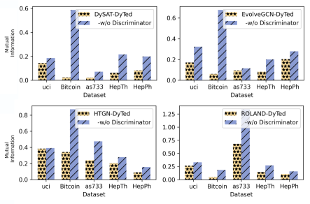
Figure 4. The discriminator can effectively minimize the mutual information between time-invariant representations and time-varying representations.

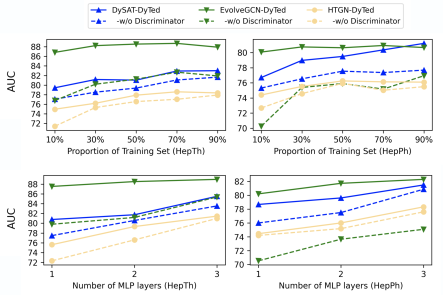
Figure 5. The performance with different training resources (training data and model complexity) for downstream tasks.

5.3.2. Evaluation of Disentangling Degree

To further quantitatively evaluate the effectiveness of the discriminator in disentangling the time-invariant and the time-varying representations, we measure the mutual information between these two types of representations. As illustrated in Figure 4, the designed discriminator is able to further reduce the mutual information between the time-invariant and the time-varying representations, resulting in a higher degree of disentanglement.

5.4. Benefit of the Disentanglement

In this section, we answer RQ3, i.e., is there any additional benefit of disentangling representation? In particular, we analyze such benefits in terms of both training resources required by downstream tasks and the robustness of models. Here we only show part of the results for the readability of figures, more results see Figure 9, Figure 10, Figure 11, and Figure 12 in Appendix A.5.

5.4.1. Training Resources

As demonstrated in Figure 5, the representation disentangled through the discriminator is able to achieve good performance with a smaller proportion of training data or a simpler downstream model. In contrast, the framework without discriminator needs more training resources to obtain a comparable or even lower performance.

5.4.2. Robustness against noise

To evaluate the robustness of our framework DyTed, we add noise to the original data by randomly adding or deleting edges for each snapshot. The ratio $r\%$ of noise refers to the proportion of added or deleted edges to existing edges, which increased from 0% to 50% in steps of 10%. As shown in Figure 6, our framework achieves better robustness, i.e., when compared with baselines, the performance of DyTed decreases less with the percentage of noise increases.

5.5. Hyper-parameter Analysis

We also analyze the effect of the hyper-parameters $\lambda_{1}$ and $\lambda_{2}$ on the performance of our proposed framework DyTed. We choose $\lambda_{1}$ and $\lambda_{2}$ from $\{0.1,0.2,...,1.0\}$, and take the LSTMGCN as an exampled backbone model. As illustrated in Figure 7, the overall performance of the framework is relatively stable.

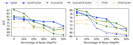
Figure 6. Performance against different noise rates.

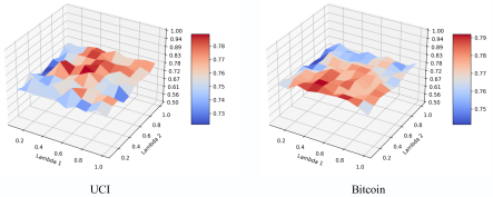
Figure 7. Hyper-parameter analysis of $\lambda_{1}$ and $\lambda_{2}$.

6. CONCLUSION

In this paper, we propose a novel disentangled representation learning framework for discrete-time dynamic graphs, namely DyTed. We propose a time-invariant representation generator with temporal clips contrastive learning, together with a time-varying generator with predefined pretext tasks. To improve the optimization efficiency, we design the bidirectional Bernoulli sampling to higher the sampling probability of cost-effective pairs in contrastive learning. Moreover, to further enhance the disentanglement of the two types of representations, we propose a disentanglement-aware discriminator under an adversarial learning framework from the perspective of information theory. Extensive experiments demonstrate the effectiveness, robustness, and generality of our framework.

In this work, due to the limitations of data, we only consider discrete-time dynamic graph representation learning methods. In the future, we devote ourselves to extending our framework to more types of dynamic graph representation learning approaches and scenarios, such as continuous-time dynamic graph methods.

7. Acknowledgments

This work is funded by the National Key R&D Program of China (2022YFB3103700, 2022YFB3103701), and the National Natural Science Foundation of China under Grant Nos. U21B2046, 62272125, 62102402. This work is also sponsored by CCF-Tencent Open Fund (RAGR20210108). Huawei Shen is also supported by Beijing Academy of Artificial Intelligence (BAAI).

Appendix A APPENDIX

A.1. Temporal-clips Sampling

We conduct the following experiments to get some intuitions for effective pairs of temporal clips for optimization. Specifically, according to whether the sampled pair of temporal clips have overlapping snapshots, we divide all pairs into two types: overlapping pairs and non-overlapping pairs. We then optimize one type of pairs with a given length of temporal clips and observe the loss changes on all types of pairs.

As shown in Figure 2, we have three interesting observations: 1). We find that, on average, optimizing non-overlapping pairs benefits more for the overall loss reduction than overlapping pairs, i.e., the yellow dotted line is lower than the blue dotted line. This phenomenon is intuitive since the pair of two overlapping temporal clips is naturally more likely to get similar representations, which may thus have less effect on the optimization of other pairs. 2). For non-overlapping pairs, optimizing long pairs are more effective than short pairs. This may be because long temporal clips cover more snapshots, forming more difficult samples for optimization. 3). For overlapping pairs, the result is reverse, that is, optimizing long pairs are less effective. This may be due to the fact that the number of overlapped snapshots will also be more in the long overlapping pair of temporal clips, resulting in less effective optimization.

A.2. Proof for Proposition 3

Proof.

First, give $Pr(M=m|L=l)=\Phi(l)^{-1}p(1-p)^{(m-1)}$ , we have the probability $Pr(X|L)$ as follows:

(14) $$Pr(X=1|L=l) =\sum_{m_{1}=1}^{l}Pr(M=m_{1}|L=l)\sum_{m_{2}=l-m_{1}+1}^{l}Pr(M=m_{2}|L=l)$$

$$=\Phi(l)^{-2}[p\cdot l(1-p)^{l-1}-(1-p)^{l}+(1-p)^{2l}],$$

$$Pr(X=0|L=l) =\sum_{m_{1}=1}^{l}Pr(M=m_{1}|L=l)\sum_{m_{2}=1}^{l-m_{1}}Pr(M=m_{2}|L=l)$$

$$=\Phi(l)^{-2}[1-(1-p)^{l}-p\cdot l(1-p)^{l-1}],$$

where $\Phi(l)=\sum_{m=1}^{l}p(1-p)^{(m-1)}$.

Since $Pr(L=l)=\dfrac{1}{T}$ , we have:

(15) $$Pr(X=1)-Pr(X=0)= \sum_{l=0}^{T}Pr(L=l)\left(Pr\left(X=1|L=l\right)-Pr\left(X=0|L=l\right)\right)$$

$$= \dfrac{1}{T}\sum_{l=0}^{T}\Phi(l)^{-2}(2pl(1-p)^{l-1}+(1-p)^{2l}-1)$$

Let $R(p,l)=2pl(1-p)^{l-1}+(1-p)^{2l}-1$ , when $l\geq 3$ and $\dfrac{2}{l+2}\leq p<1$ , we have $\nabla_{p}R(p,l)\leq 0$ , and $\nabla_{l}R(p,l)\leq 0$. Then:

(16) $$Pr(X=1)-Pr(X=0)\leq\dfrac{1}{T}\sum\Phi(l)^{-2}(R(p=\dfrac{2}{5},l=3))\leq 0$$

In other words, we have:

(17) $$\dfrac{Pr(X=1)}{Pr(X=0)}\leq 1$$

Accroding to Eq. 14:

(18) $$\dfrac{Pr(L=l+1|X=1)}{Pr(L=l|X=1)}= \dfrac{\Phi(l)^{2}Pr(L=l+1)}{\Phi(l+1)^{2}Pr(L=l)}$$

$$\cdot\dfrac{p\cdot(l+1)(1-p)^{l}-(1-p)^{l+1}+(1-p)^{2l+2}}{p\cdot l(1-p)^{l-1}-(1-p)^{l}+(1-p)^{2l}}$$

Since $0<\dfrac{\Phi(l)^{2}}{\Phi(l+1)^{2}}\leq 1$ , and $\dfrac{Pr(L=l+1|X=1)}{Pr(L=l|X=1)}\geq 0$ , the Eq. 18 can be written as:

(19) $$\dfrac{Pr(L=l+1|X=1)}{Pr(L=l|X=1)}\leq \dfrac{p\cdot(l+1)(1-p)^{l}-(1-p)^{l+1}+(1-p)^{2l+2}}{p\cdot l(1-p)^{l-1}-(1-p)^{l}+(1-p)^{2l}}$$

$$= \dfrac{p\cdot l(1-p)^{l}-(1-p)^{l+1}+(1-p)^{2l+2}+p(1-p)^{l}}{p\cdot l(1-p)^{l-1}-(1-p)^{l}+(1-p)^{2l}}$$

$$\leq (1-p)+\dfrac{p(1-p)^{l}}{p\cdot l(1-p)^{l-1}-(1-p)^{l}+(1-p)^{2l}}$$

$$\leq (1-p)+\dfrac{p(1-p)^{l}}{p\cdot l(1-p)^{l-1}-(1-p)^{l}}$$

$$= 1+\dfrac{p\left(2-p\left(l+2\right)\right)}{p\cdot\left(l+1\right)-1}$$

Given that $\dfrac{2}{l+2}\leq p<1$ , we have $\left(2-p\left(l+2\right)\right)\leq 0$ and $p\cdot\left(l+1\right)-1>0$ . Then we have:

(20) $$\dfrac{Pr(L=l+1|X=1)}{Pr(L=l|X=1)}=\dfrac{Pr(X=1|L=l+1)}{Pr(X=1|L=l)}\leq 1$$

Since $Pr(X=1|L=l)+Pr(X=0|L=l)=1$, we then have:

(21) $$\dfrac{Pr(L=l+1|X=0)}{Pr(L=l|X=0)}=\dfrac{Pr(X=0|L=l+1)}{Pr(X=0|L=l)}=\dfrac{1-Pr(X=1|L=l+1)}{1-Pr(X=1|L=l)}\geq 1$$

By combining Formula 17, 20, and 21, the proposition is proved.

∎

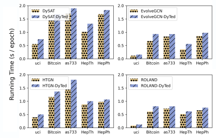
Figure 8. Running time of baselines and our framework.

Table 6. Node classification for Pooling Representation

Model	Assets		Financing Risk
	micro-F1	macro-F1	micro-F1	macro-F1
LSTMGCN	24.06 $\pm$ 0.46	16.37 $\pm$ 0.39	49.13 $\pm$ 0.32	29.56 $\pm$ 0.64
LSTMGCN-Pooling1	23.07 $\pm$ 0.35	13.94 $\pm$ 0.13	47.19 $\pm$ 0.23	22.25 $\pm$ 0.13
DySAT	25.50 $\pm$ 0.58	13.06 $\pm$ 0.46	42.95 $\pm$ 2.46	25.03 $\pm$ 0.74
DySAT-Pooling	22.85 $\pm$ 0.66	12.76 $\pm$ 0.27	34.51 $\pm$ 1.22	26.13 $\pm$ 0.92
EvolveGCN	24.39 $\pm$ 1.02	11.62 $\pm$ 0.17	43.76 $\pm$ 1.00	25.76 $\pm$ 0.40
EvolveGCN-Pooling	26.02 $\pm$ 2.23	8.76 $\pm$ 0.20	34.21 $\pm$ 0.15	16.99 $\pm$ 0.52
HTGN	26.70 $\pm$ 0.39	11.25 $\pm$ 0.71	50.13 $\pm$ 0.19	22.26 $\pm$ 0.06
HTGN-Pooling	25.45 $\pm$ 0.67	8.66 $\pm$ 0.31	50.15 $\pm$ 0.22	21.36 $\pm$ 0.79
ROLAND	28.08 $\pm$ 0.43	8.77 $\pm$ 0.10	49.34 $\pm$ 0.42	22.02 $\pm$ 0.12
ROLAND-Pooling	27.98 $\pm$ 0.13	8.71 $\pm$ 0.36	47.41 $\pm$ 0.93	21.31 $\pm$ 0.66

• The pooling of the representations over all snapshots of the baselines.

Table 7. Link prediction

Model	Uci		Bitcoin		as733		HepTh		HepPh
	AUC	AP	AUC	AP	AUC	AP	AUC	AP	AUC	AP
LSTMGCN-Time-invariant1	71.73 $\pm$ 0.68	69.05 $\pm$ 1.5	64.75 $\pm$ 0.48	64.71 $\pm$ 0.4	73.16 $\pm$ 0.13	72.56 $\pm$ 0.28	75.09 $\pm$ 0.71	74.89 $\pm$ 0.73	78.99 $\pm$ 0.72	78.74 $\pm$ 0.83
LSTMGCN-Time-varying	70.08 $\pm$ 0.42	70.09 $\pm$ 1.33	75.1 $\pm$ 0.62	74.94 $\pm$ 0.61	74.53 $\pm$ 1.15	73.94 $\pm$ 1.27	81.02 $\pm$ 0.16	81.15 $\pm$ 0.14	78.91 $\pm$ 0.36	79.78 $\pm$ 0.39
DySAT-Time-invariant	81.84 $\pm$ 0.44	81.56 $\pm$ 0.39	74.48 $\pm$ 1.47	74.28 $\pm$ 1.46	77.48 $\pm$ 1.32	77.61 $\pm$ 1.31	71.43 $\pm$ 0.89	72.04 $\pm$ 0.87	61.65 $\pm$ 0.68	61.8 $\pm$ 0.72
DySAT-Time-varying	80.16 $\pm$ 0.85	79.2 $\pm$ 0.65	76.27 $\pm$ 0.85	76.62 $\pm$ 0.81	72.77 $\pm$ 0.13	73.34 $\pm$ 0.13	73.31 $\pm$ 1.19	71.26 $\pm$ 1.23	77.4 $\pm$ 1.64	77.36 $\pm$ 1.66
EvolveGCN-Time-invariant	83.98 $\pm$ 0.87	89.11 $\pm$ 0.82	81.91 $\pm$ 0.46	82.02 $\pm$ 0.44	75.52 $\pm$ 0.35	73.5 $\pm$ 2.31	72.93 $\pm$ 1.91	73.42 $\pm$ 1.93	69.37 $\pm$ 1.76	69.46 $\pm$ 1.72
EvolveGCN-Time-varying	56.66 $\pm$ 0.47	57.54 $\pm$ 0.81	69.64 $\pm$ 1.53	69.73 $\pm$ 1.57	70.51 $\pm$ 1.82	70.93 $\pm$ 1.85	79.88 $\pm$ 1.45	79.59 $\pm$ 1.43	67.8 $\pm$ 2.04	68.01 $\pm$ 2.08
HTGN-Time-invariant	91.57 $\pm$ 0.12	90.17 $\pm$ 0.38	84.33 $\pm$ 0.29	83.92 $\pm$ 0.2	76.51 $\pm$ 0.14	76.32 $\pm$ 0.29	72.59 $\pm$ 0.93	72.86 $\pm$ 0.97	72.65 $\pm$ 0.67	72.48 $\pm$ 0.62
HTGN-Time-varying	80.73 $\pm$ 0.32	79.67 $\pm$ 0.36	87.01 $\pm$ 0.49	88.07 $\pm$ 0.48	72.14 $\pm$ 0.27	72.29 $\pm$ 0.39	75.56 $\pm$ 0.35	75.82 $\pm$ 0.35	70.6 $\pm$ 0.86	70.65 $\pm$ 0.86
ROLAND-Time-invariant	69.7 $\pm$ 1.12	67.37 $\pm$ 1.21	73.08 $\pm$ 2.01	73.06 $\pm$ 2.21	73.96 $\pm$ 0.26	74.25 $\pm$ 0.12	79.47 $\pm$ 0.21	79.53 $\pm$ 0.12	79.39 $\pm$ 0.37	78.78 $\pm$ 0.31
ROLAND-Time-varying	87.01 $\pm$ 0.93	87.21 $\pm$ 0.63	88.61 $\pm$ 0.05	88.62 $\pm$ 0.12	74.63 $\pm$ 0.35	74.11 $\pm$ 0.13	80.11 $\pm$ 0.6	79.67 $\pm$ 0.39	80.47 $\pm$ 0.51	79.97 $\pm$ 0.29

• baseline-Time-invariant and baseline-Time-Varying are under our framework DyTed.

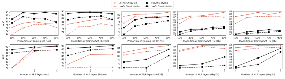
Figure 9. The benefits of disentanglement in terms of training resources for LSTMGCN and ROLAND.

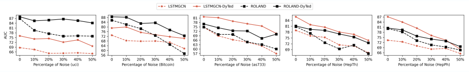
Figure 10. Performance against different noise rates for LSTMGCN and ROLAND.

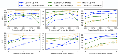
Figure 11. The benefits of disentanglement in terms of training resources.

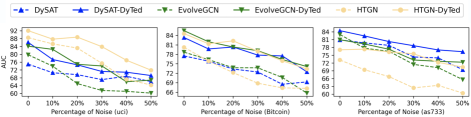
Figure 12. Performance against different noise rates.

A.3. Running Time Comparison

Figure 8 demonstrates the running time between baselines and our framework DyTed, which is comparable in order of magnitude.

A.4. Performance of Pooling Representation

Table 6 demonstrates the performance of pooling representations among all snapshots for node classification, showing a worse $F1$ than the representation of the last snapshot. (Due to the space limitation, we only show the results on two labels.)

A.5. Supplement

We have included Table 7 to supplement Table 4 in Section 5.2, Figure 9, Figure 10, Figure 11, and Figure 12 to supplement Figure 5 and Figure 6 in Section 5.4. These additional tables support the same conclusions.

References

- (1)
- Ahmed et al. (2018) Nahla Mohamed Ahmed, Ling Chen, Yulong Wang, Bin Li, Yun Li, and Wei Liu. 2018. DeepEye: Link prediction in dynamic networks based on non-negative matrix factorization. Big Data Mining and Analytics (2018), 19–33.
- Bai et al. (2018) Shaojie Bai, J Zico Kolter, and Vladlen Koltun. 2018. An empirical evaluation of generic convolutional and recurrent networks for sequence modeling. In arXiv preprint arXiv:1803.01271.
- Cai et al. (2021) Lei Cai, Zhengzhang Chen, Chen Luo, Jiaping Gui, Jingchao Ni, Ding Li, and Haifeng Chen. 2021. Structural temporal graph neural networks for anomaly detection in dynamic graphs. In Proceedings of the 30th ACM International Conference on Information and Knowledge Management. 3747–3756.
- Cao et al. (2022) Jiangxia Cao, Xixun Lin, Xin Cong, Jing Ya, Tingwen Liu, and Bin Wang. 2022. DisenCDR: Learning disentangled representations for cross-Domain recommendation. In Proceedings of the 45th International ACM SIGIR Conference on Research and Development in Information Retrieval. 267–277.
- Cao et al. (2015) Shaosheng Cao, Wei Lu, and Qiongkai Xu. 2015. GraRep: Learning graph representations with global structural information. In Proceedings of the 24th ACM International Conference on Information and Knowledge Management. 891–900.
- Cen et al. (2019) Keting Cen, Huawei Shen, Jinhua Gao, Qi Cao, Bingbing Xu, and Xueqi Cheng. 2019. Anae: Learning node context representation for attributed network embedding. arXiv preprint arXiv:1906.08745 (2019).
- Chang et al. (2020) Xiaofu Chang, Xuqin Liu, Jianfeng Wen, Shuang Li, Yanming Fang, Le Song, and Yuan Qi. 2020. Continuous-time dynamic graph learning via neural interaction processes. In Proceedings of the 29th ACM International Conference on Information and Knowledge Management. 145–154.
- Chen et al. (2021) Hong Chen, Yudong Chen, Xin Wang, Ruobing Xie, Rui Wang, Feng Xia, and Wenwu Zhu. 2021. Curriculum disentangled recommendation with noisy multi-feedback. In Proceedings of the 35th Conference on NeurIPS. 26924–26936.
- Cui et al. (2019) Peng Cui, Xiao Wang, Jian Pei, and Wenwu Zhu. 2019. A survey on network embedding. IEEE Transactions on Knowledge and Data Engineering (2019), 833–852.
- Goyal et al. (2018) Palash Goyal, Nitin Kamra, Xinran He, and Yan Liu. 2018. Dyngem: Deep embedding method for dynamic graphs. In arXiv preprint arXiv:1805.11273.
- Jang et al. (2016) Eric Jang, Shixiang Gu, and Ben Poole. 2016. Categorical reparameterization with gumbel-softmax. arXiv preprint arXiv:1611.01144 (2016).
- John et al. (2019) Vineet John, Lili Mou, Hareesh Bahuleyan, and Olga Vechtomova. 2019. Disentangled representation learning for non-parallel text style transfer. In Proceedings of the 57th Annual Meeting of the ACL. 424–434.
- Kipf and Welling (2016) Thomas N Kipf and Max Welling. 2016. Semi-supervised classification with graph convolutional networks. In Proceedings of the 4th International Conference on Learning Representations.
- Kumar et al. (2018) Srijan Kumar, Bryan Hooi, Disha Makhija, Mohit Kumar, Christos Faloutsos, and VS Subrahmanian. 2018. Rev2: Fraudulent user prediction in rating platforms. In Proceedings of the Eleventh ACM International Conference on WSDM. ACM, 333–341.
- Kumar et al. (2019) Srijan Kumar, Xikun Zhang, and Jure Leskovec. 2019. Predicting dynamic embedding trajectory in temporal interaction networks. In Proceedings of the 25th ACM SIGKDD international conference on knowledge discovery and data mining. 1269–1278.
- Leskovec et al. (2005) Jure Leskovec, Jon Kleinberg, and Christos Faloutsos. 2005. Graphs over time: densification laws, shrinking diameters and possible explanations. In Proceedings of the 11th ACM SIGKDD Conference on Knowledge Discovery and Data Mining. 177–187.
- Li et al. (2022) Fuxian Li, Jie Feng, Huan Yan, Guangyin Jin, Fan Yang, Funing Sun, Depeng Jin, and Yong Li. 2022. Dynamic graph convolutional recurrent network for traffic prediction: benchmark and solution. ACM Transactions on Knowledge Discovery from Data (2022), 1–21.
- Li et al. (2017) Jundong Li, Harsh Dani, Xia Hu, Jiliang Tang, Yi Chang, and Huan Liu. 2017. Attributed network embedding for learning in a dynamic environment. In Proceedings of the 26th ACM International Conference on Information and Knowledge Management. 387–396.
- Liu et al. (2019) Yozen Liu, Xiaolin Shi, Lucas Pierce, and Xiang Ren. 2019. Characterizing and forecasting user engagement with in-app action graph: A case study of snapchat. In Proceedings of the 25th ACM SIGKDD Conference on Knowledge Discovery and Data Mining. 2023–2031.
- Locatello et al. (2019) Francesco Locatello, Stefan Bauer, Mario Lucic, Gunnar Raetsch, Sylvain Gelly, Bernhard Schölkopf, and Olivier Bachem. 2019. Challenging Common Assumptions in the Unsupervised Learning of Disentangled Representations. In Proceedings of the 36th International Conference on Machine Learning. 4114–4124.
- Ma et al. (2019) Jianxin Ma, Peng Cui, Kun Kuang, Xin Wang, and Wenwu Zhu. 2019. Disentangled graph convolutional networks. In Proceedings of the 36th International Conference on Machine Learning. 4212–4221.
- Nguyen et al. (2018a) Giang Hoang Nguyen, John Boaz Lee, Ryan A. Rossi, Nesreen K. Ahmed, Eunyee Koh, and Sungchul Kim. 2018a. Continuous-time dynamic network embeddings. In Companion Proceedings of the 28th ACM Web Conference. 969–976.
- Nguyen et al. (2018b) Giang H Nguyen, John Boaz Lee, Ryan A Rossi, Nesreen K Ahmed, Eunyee Koh, and Sungchul Kim. 2018b. Dynamic network embeddings: From random walks to temporal random walks. In Proceedings of the 3rd IEEE International Conference on Big Data. 1085–1092.
- Oord et al. (2018) Aaron van den Oord, Yazhe Li, and Oriol Vinyals. 2018. Representation learning with contrastive predictive coding. In arXiv preprint arXiv:1807.03748.
- Panzarasa et al. (2009) Pietro Panzarasa, Tore Opsahl, and Kathleen M Carley. 2009. Patterns and dynamics of users’ behavior and interaction: Network analysis of an online community. Journal of the American Society for Information Science and Technology (2009), 911–932.
- Pareja et al. (2020) Aldo Pareja, Giacomo Domeniconi, Jie Chen, Tengfei Ma, Toyotaro Suzumura, Hiroki Kanezashi, Tim Kaler, Tao Schardl, and Charles Leiserson. 2020. Evolvegcn: Evolving graph convolutional networks for dynamic graphs. In Proceedings of the 34th AAAI Conference on Artificial Intelligence. 5363–5370.
- Sankar et al. (2020) Aravind Sankar, Yanhong Wu, Liang Gou, Wei Zhang, and Hao Yang. 2020. Dysat: Deep neural representation learning on dynamic graphs via self-attention networks. In Proceedings of the 13th International Conference on WSDM. 519–527.
- Tian et al. (2021) Sheng Tian, Ruofan Wu, Leilei Shi, Liang Zhu, and Tao Xiong. 2021. Self-supervised representation learning on dynamic graphs. In Proceedings of the 30th ACM International Conference on Information and Knowledge Management. 1814–1823.
- Tran et al. (2017) Luan Tran, Xi Yin, and Xiaoming Liu. 2017. Disentangled representation learning GAN for pose-invariant face recognition. In Proceedings of the 27th IEEE CVPR.
- Trivedi et al. (2019) Rakshit Trivedi, Mehrdad Farajtabar, Prasenjeet Biswal, and Hongyuan Zha. 2019. Dyrep: Learning representations over dynamic graphs. In Proceedings of the 7th International Conference on Learning Representations.
- Vaswani et al. (2017) Ashish Vaswani, Noam Shazeer, Niki Parmar, Jakob Uszkoreit, Llion Jones, Aidan N Gomez, Łukasz Kaiser, and Illia Polosukhin. 2017. Attention is all you need. In Proceedings of the 31th Conference on NeurIPS. 30.
- Velickovic et al. (2017) Petar Velickovic, Guillem Cucurull, Arantxa Casanova, Adriana Romero, Pietro Lio, and Yoshua Bengio. 2017. Graph attention networks. In Proceedings of the 5th International Conference on Learning Representations.
- Wang et al. (2020) Yanbang Wang, Pan Li, Chongyang Bai, V Subrahmanian, and Jure Leskovec. 2020. Generic representation learning for dynamic social interaction. In Proceedings of the 26th ACM SIGKDD Conference on Knowledge Discovery and Data Mining Workshop.
- Wang et al. (2022) Yifan Wang, Yifang Qin, Fang Sun, Bo Zhang, Xuyang Hou, Ke Hu, Jia Cheng, Jun Lei, and Ming Zhang. 2022. DisenCTR: Dynamic graph-based disentangled representation for click-through rate prediction. In Proceedings of the 45th International ACM SIGIR Conference on Research and Development in Information Retrieval. 2314–2318.
- Xu et al. (2020) Da Xu, Chuanwei Ruan, Evren Korpeoglu, Sushant Kumar, and Kannan Achan. 2020. Inductive representation learning on temporal graphs. arXiv preprint arXiv:2002.07962 (2020).
- Xue et al. (2022) Guotong Xue, Ming Zhong, Jianxin Li, Jia Chen, Chengshuai Zhai, and Ruochen Kong. 2022. Dynamic network embedding survey. Neurocomputing (2022), 212–223.
- Yang et al. (2021) Menglin Yang, Min Zhou, Marcus Kalander, Zengfeng Huang, and Irwin King. 2021. Discrete-time temporal network embedding via implicit hierarchical learning in hyperbolic space. In Proceedings of the 27th ACM SIGKDD Conference on Knowledge Discovery and Data Mining. 1975–1985.
- You et al. (2022) Jiaxuan You, Tianyu Du, and Jure Leskovec. 2022. ROLAND: Graph learning framework for dynamic graphs. In Proceedings of the 28th ACM SIGKDD Conference on Knowledge Discovery and Data Mining. 2358–2366.
- Yu et al. (2018) Wenchao Yu, Wei Cheng, Charu C Aggarwal, Kai Zhang, Haifeng Chen, and Wei Wang. 2018. Netwalk: A flexible deep embedding approach for anomaly detection in dynamic networks. In Proceedings of the 24th ACM SIGKDD Conference on Knowledge Discovery and Data Mining. 2672–2681.
- Zhang et al. (2019) Yizhou Zhang, Guojie Song, Lun Du, Shuwen Yang, and Yilun Jin. 2019. DANE: Domain adaptive network embedding. In Proceedings of the 28th International Joint Conference on Artificial Intelligence. 4362–4368.
- Zhao et al. (2022) Tianxiang Zhao, Xiang Zhang, and Suhang Wang. 2022. Exploring edge disentanglement for node classification. In Proceedings of the 32nd ACM Web Conference. 1028–1036.
- Zhou et al. (2018) Lekui Zhou, Yang Yang, Xiang Ren, Fei Wu, and Yueting Zhuang. 2018. Dynamic network embedding by modeling triadic closure process. In Proceedings of the 32nd Proceedings of the AAAI Conference on Artificial Intelligence.
- Zhu et al. (2021) Xinqi Zhu, Chang Xu, and Dacheng Tao. 2021. Where and what? examining interpretable disentangled representations. In Proceedings of the IEEE/CVF Conference on CVPR. 5861–5870.
- Zhu et al. (2020) Yanqiao Zhu, Yichen Xu, Feng Yu, Qiang Liu, Shu Wu, and Liang Wang. 2020. Deep graph contrastive representation learning. In arXiv preprint arXiv:2006.04131.
- Zuo et al. (2018) Yuan Zuo, Guannan Liu, Hao Lin, Jia Guo, Xiaoqian Hu, and Junjie Wu. 2018. Embedding temporal network via neighborhood formation. In Proceedings of the 24th ACM SIGKDD Conference on Knowledge Discovery and Data Mining. 2857–2866.