Margin Optimal Classification Trees

Abstract

In recent years, there has been growing attention to interpretable machine learning models which can give explanatory insights on their behaviour. Thanks to their interpretability, decision trees have been intensively studied for classification tasks and, due to the remarkable advances in mixed integer programming (MIP), various approaches have been proposed to formulate the problem of training an Optimal Classification Tree (OCT) as a MIP model. We present a novel mixed integer quadratic formulation for the OCT problem, which exploits the generalization capabilities of Support Vector Machines for binary classification. Our model, denoted as Margin Optimal Classification Tree (MARGOT), encompasses maximum margin multivariate hyperplanes nested in a binary tree structure. To enhance the interpretability of our approach, we analyse two alternative versions of MARGOT, which include feature selection constraints inducing sparsity of the hyperplanes’ coefficients. First, MARGOT has been tested on non-linearly separable synthetic datasets in a 2-dimensional feature space to provide a graphical representation of the maximum margin approach. Finally, the proposed models have been tested on benchmark datasets from the UCI repository. The MARGOT formulation turns out to be easier to solve than other OCT approaches, and the generated tree better generalizes on new observations. The two interpretable versions effectively select the most relevant features, maintaining good prediction quality.

© 2023. Licensed under the Creative Commons CC-BY-NC-ND 4.0.

1 Introduction

1.1 Related Work

In recent years, there has been growing interest in interpretable Machine Learning (ML) models [43]. Decision trees are among the most popular Supervised ML tools used for classification tasks. They are famous for being easy to manage, having low computational requirements, and the final model is easily understandable from a human perspective as opposed to other ML methods that are seen as black boxes. Given a set of points and class labels, a classification tree method builds up a binary tree structure of a maximum predefined depth. Trees are composed of branch and leaf nodes, and the branch nodes apply a sequence of dichotomic rules, called splitting rules, to partition the training samples into disjoint subsets. Splitting rules route samples to the left or right child node, and they are usually defined by hyperplanes. In a univariate tree, these hyperplanes are orthogonal, involving one single feature, while in a multivariate tree, they can be oblique, involving more than one feature. A value for the predicted class label is assigned to each leaf node according to some simple rule, for instance, the most common label rule. The key advantage of tree methods lies in their interpretability. The process behind a decision tree is transparent, and the sequential tree structure mimics the human decision-making process. These properties can be crucial factors in many applications, ranging from business and criminal justice to healthcare and bioinformatics. Indeed, in these domains, it is of great interest to use explainable approaches to help humans understand the model’s decisions and identify a subset of the most prominent features that influence the classification outcome. To this aim, it is preferable to build and manage shallow trees with small depth; indeed, if allowed to grow large, decision trees lose their interpretability aspect.

It is well-known that constructing a binary decision tree in an optimal way is an NP-complete problem [31]. For this reason, traditional approaches for finding decision trees rely on heuristics. In general, they are based on a top-down greedy strategy for growing the tree by generating splits at each node, and, once the tree is built, a bottom-up pruning procedure is applied to handle the complexity of the tree, i.e. the number of splits. Breiman et al. [16] proposed a heuristic algorithm known as CART (Classification and Regression Trees) for learning univariate decision trees. Starting from the root node, each hyperplane split is generated by minimizing a local impurity function, e.g. the Gini impurity for classification tasks.

Other univariate approaches employing different impurity functions were later proposed by Quinlan [41, 42] in his ID3 and C4.5 algorithms. These heuristic procedures produce a solution in fast computational time but may also generate tree models with poor generalization performances. In order to overcome these drawbacks, tree ensemble methods, such as Random Forests [15], TreeBoost [26] and XGBoost [22], have been proposed. These approaches combine decision trees using some kind of randomness; however, using multiple trees leads to a lack of interpretability of the final model.

Another way to improve prediction quality is to use multivariate decision trees, which employ oblique hyperplane splits. These methods involve more features per split, thus producing smaller trees but at the expense of the computational cost. Several approaches for inducing multivariate trees have been proposed (see [38, 17, 39, 49]). For instance, OC1 [38] is a greedy algorithm that searches for the best hyperplane at each node by applying a randomized perturbation strategy. In contrast, [39] presented a heuristic procedure that, at each step, solves a variant of the Support Vector Machine problem, where the empirical error is discretized by counting the number of misclassified samples.

Recently, several papers have been devoted to global exact optimization approaches to find an Optimal Classification Tree (OCT) using mathematical programming tools and, in particular, Mixed Integer Programming (MIP) models (see the recent surveys [27, 19] and references therein). Indeed, the significant improvement in the last thirty years of both algorithms for integer optimization and computer hardware has led to an incredible increase in the computational power of mixed integer solvers, as shown in [7]. Thus, MIP approaches became viable in the definition of ML methods, being [6] the seminal paper inaugurating a new era in using mixed integer based optimization to learn OCTs. Such approaches find the decision tree in its entirety through the resolution of a single optimization model, defining each branching rule with full knowledge of all the remaining ones. In [6], Bertsimas and Dunn proposed two Mixed Integer Linear Programming (MILP) models to build optimal trees with a given maximum depth based on univariate and multivariate splits. Along these lines, Günlük et al. [28] proposed a MIP formulation for binary classification tasks by exploiting the structure of categorical features and modelling combinatorial decisions. Further, in order to circumvent the problem of the curse of dimensionality related to the MIP approaches, Verwer and Zhang [46] presented BinOCT, a binary linear programming model, where the size is independent of the training set dimension. In [2], Aghaei et al. proposed a flow-based MILP model for binary features with a stronger linear relaxation and, by exploiting the decomposable and combinatorial structure of the model, derived a Benders’ decomposition method to deal with larger instances. Boutilier et al. [13] presented a new formulation for learning multivariate optimal trees. Moreover, they introduced a new class of valid inequalities and leveraged them within a Benders-like decomposition to improve the optimization process. In addition to expressing the combinatorial nature of the decisions involved in the process, the mixed integer framework is suitable to handle global objectives and constraints to embed desirable properties such as fairness, sparsity, cost-sensitivity, robustness, as it has been addressed in [19], [45], [1], [2] and [9].

Alongside integer optimization, continuous optimization paradigms have also been investigated in the context of optimal trees. In [12], Blanquero et al. proposed a nonlinear programming model for learning an optimal ”randomized” classification tree with oblique splits, where at each node, a random decision is made according to a soft rule, induced by a continuous cumulative density function. Later, in [11], they addressed global and local sparsity in the randomized optimal tree model (S-ORCT) by means of regularization terms based on polyhedral norms ($\ell_{1}$-norm and $\ell_{\infty}$-norm). In their randomized framework, a sample is not assigned to a class in a deterministic way but only with a given probability. Following this research line, Amaldi et al. [4] investigated additional versions of the S-ORCT model based on concave approximations of the $\ell_{0}$-norm and proposed a general proximal point decomposition scheme to tackle larger datasets.

Following a different viewpoint, approaches using a Support Vector Machine (SVM) (see [23], [47], [40]) for each split in the tree have been investigated. First, Bennett et al. [5] provided a primal continuous formulation with a non-convex objective function and a dual convex quadratic model to train optimal trees where each decision rule is based on a modified SVM problem. Their model can involve kernel functions to construct nonlinear splitting rules. The resulting problems are computationally hard to solve, and a tabu search algorithm is used to approximately find solutions. Recently, margin-based splits of the SVM type have been proposed by Blanco et al. in [9]. The authors introduced a Mixed Integer Nonlinear formulation for the OCT problem to solve binary classification tasks. The aim was to build a robust tree classifier, where during the training phase, some of the labels of the dataset are allowed to be changed in order to detect the label noise. Observations are relabelled based on misclassification errors, as described in [8]. The method aims to seek a trade-off between four objectives, the first being the maximization of the minimum margin among all the margins of the hyperplane splits in the tree. In addition, it minimizes the misclassification cost at the branch nodes, the number of relabelled observations and the complexity of the tree. The model is formulated as a Mixed Integer Second Order Cone Optimization problem. In [10], an extension of the model in [9] for handling multiclass instances has been proposed.

1.2 Our contribution

Our approach falls within the basic framework of using Support Vector Machines to define optimal classification trees with multivariate splits for binary classification tasks. In particular, our model employs maximum margin hyperplanes obtained using a linear soft SVM paradigm in a nested binary tree structure. The maximum depth of the tree is fixed, as usual in OCT approaches.

The main contribution of this paper is a novel Mixed Integer Quadratic Programming (MIQP) formulation, denoted as Margin Optimal Classification Tree (MARGOT), for learning classification trees. Our formulation differs from others in the literature as we exploit the statistical learning properties of the $\ell_{2}$-regularized soft SVM formulation. In particular, the SVM quadratic convex function is retained, and the collective measure of performance of the OCT is obtained as the sum of the objective functions of each SVM-based problem over all the branch nodes of the tree. Differently, in [9], only the minimum among all the hyperplane margins is maximized. Further, exploiting both the SVMs properties and the binary classification setting allows us to drastically reduce the overall number of binary variables needed in our MIQP model. Specifically, we need to introduce as many binary variables as half the number of leaf nodes, which is much less than other OCT MIP approaches. We show, both on synthetic datasets in a 2-dimensional feature space and on datasets selected from the UCI Machine Learning repository [24], that MARGOT formulation requires less computational effort than other state-of-the-art MIP models for OCT, and it can be solved to certified optimality on nearly all the considered problems with a limited computational time using off-the-shelf solvers. As a consequence of the maximum margin approach, our model produces OCTs with a higher out-of-sample accuracy.

As a second contribution, we aim to reduce the number of features used in each split to enhance the interpretability of the model itself. Indeed, for tabular data, sparsity is a core component of interpretability [43], and having fewer features selected at each branching node allows the end user to identify the key factors affecting the classification of the samples.

Actually, due to the intrinsic statistical properties of SVMs, such a model tends to use a large number of features to define each split of the classification tree. For this reason, we propose two embedded models that simultaneously train the OCT and perform feature selection. Embedded models for feature selection in SVMs have been studied in several papers (see e.g. [32, 20, 36, 33, 34]). To control the sparsity of the oblique splits, we draw inspiration from the model proposed in [33], and we use additional binary variables and a budget on the number of features used. We consider two different modellings of the budget on the number of features: hard constraints and soft penalization, respectively implemented in HFS-MARGOT and SFS-MARGOT. Numerical results on the UCI datasets are reported, showing that the hard version seems to be easier to solve to certified optimality in a reasonable CPU time, resulting in a more sparse solution too. For all the formulations, we propose a simple greedy heuristic to obtain a first incumbent which exploits the SVM-based tree structure.

The rest of the paper is organized as follows. In Section 2, a brief introduction about Multivariate Optimal Classification Trees, proposed in [6], and Support Vector Machines is provided. In Section 3, we introduce our approach and its formulation, denoted as MARGOT. In Section 4, we present the two interpretable versions of the model with hard and soft feature selection techniques to address the sparsity of the hyperplanes’ weights. In Section 5, we provide a heuristic to generate starting feasible solutions for the analysed MIP problems. Then, in Section 6, we first evaluate MARGOT on 2-dimensional synthetic datasets, and we report a graphical representation of the generated trees. Finally, computational experiments on benchmark datasets from the UCI repository are presented for all the proposed models.

2 Preliminaries

2.1 Multivariate Optimal Classification Trees

In this section, we introduce in more detail multivariate optimal classification trees. Given a dataset $\{(x^{i},y^{i})\in\mathbb{R}^{n}\times\{1,\dots,K\},\ i\in\mathcal{I}\}$, and a maximum depth $D$, an optimal classification tree is made up by $2^{(D+1)}-1$ nodes, divided in:

• Branch nodes, $\mathcal{T}_{B}=\{0,\dots,2^{D}-2\}$: a branch node applies a splitting rule on the feature space defined by a separating hyperplane $\mathcal{H}_{t}(x):=\{x:h_{t}(x)=0\}$, where $h_{t}(x)=w^{T}_{t}x+b_{t}$ is the hyperplane function and $w_{t}\in\mathbb{R}^{n}$ and $b_{t}\in\mathbb{R}$. If $h_{t}(x^{i})\geq 0$, sample $i$ will follow the right branch of node $t$, otherwise it will follow the left one;

• Leaf nodes, $\mathcal{T}_{L}=\{2^{D}-1,\dots,2^{D+1}-2\}$: leaf nodes act as collectors, and the samples which end up in the same leaf are classified with the same class label.

The training phase aims at building a classification tree by finding coefficients $w_{t}$ and the intercept $b_{t}$ for each $t\in\mathcal{T}_{B}$ and by assigning class labels to the leaf nodes. According to the hierarchical tree structure, the feature space will be partitioned into disjoint regions, each corresponding to a leaf node of the tree. The obtained tree is then used to classify out-of-sample data: every new sample will follow a unique path within the tree based on the splitting rules, ending up in a leaf node that will predict its class label.

In [6], Bertsimas and Dunn proposed a MILP optimization model for training multivariate OCTs, denoted as OCT-H, where, in the objective function, the misclassification error together with the number of features used at each split is minimized. In the optimization model, each sample is forced to end up in a single leaf, a class label for each leaf node is chosen according to the most common label rule and the classification error is computed according to the assignment of each sample to a leaf. Routing constraints enforce each sample to follow a unique path, while other constraints control the complexity of the tree by imposing pruning conditions and a minimum number of points accepted by each non-empty leaf.

2.2 A brief overview on Support Vector Machines

Given a binary classification instance $\{(x^{i},y^{i})\in\mathbb{R}^{n}\times\{-1,1\},\ i\in\mathcal{I}\}$, the linear soft-margin SVM classification problem defines a linear classifier as the function $f:\mathbb{R}^{n}\to\{-1,1\}$,

$$f(x)=\mbox{\rm sgn}({w^{*}}^{T}x+b^{*}),$$

using the structural risk minimization principle ([23, 44]). In the traditional $\ell_{2}$-regularized $\ell_{1}$-loss linear SVM, coefficients $(w^{*},b^{*})\in\mathbb{R}^{n}\times\mathbb{R}$ identify a separating hyperplane that maximizes its margin, i.e. the distance between two parallel hyperplanes, each supporting samples belonging to one of the two classes. The tuple is found by solving the following convex quadratic problem:

$$\text{(SVM})\quad\min\limits_{{w,b,\xi}}\quad \displaystyle\frac{1}{2}\|w\|^{2}_{2}+C\sum_{i\in\mathcal{I}}\xi_{i}$$ (1)

s.t. $$y^{i}(w^{T}x^{i}+b)\geq 1-\xi_{i} \forall i\in\mathcal{I}$$ (2)

$$\xi_{i}\geq 0 \forall i\in\mathcal{I},$$

where $C$ is a hyperparameter that balances the two objectives: the maximization of the margin $2\|w\|_{2}^{-1}$ and the minimization of the misclassification cost. Variables $\xi_{i}$ allow for violation of the margin constraints (2) and a sample $i$ is misclassified when $\xi_{i}>1$, while values $0<\xi_{i}\leq 1$ correspond to correctly classified samples inside the margin. The further a misclassified data point $x^{i}$ is from a feasible hyperplane, the greater the value of variable $\xi_{i}$ will be (see Fig. 1). Thus, $\sum_{i\in\mathcal{I}}\xi_{i}$ is an upper bound on the number of samples misclassified by the hyperplane.

Figure 1: Example showing how errors are upper-bounded in the SVM approach by variables $\xi_{i}$: values $0<\xi_{i}\leq 1$ correspond to samples that lie within the margin but are correctly classified; values $\xi_{i}>1$ correspond to samples wrongly classified.

Although the objective function of the SVM problem is loosely convex, in [18], necessary and sufficient conditions are given for the support vector solution to be unique. In particular, with reference to (1) where $C$ is the same for all $i$, a necessary condition for the solution to be non-unique is that the negative and positive polarity support vectors are equal in number. Further, it has been proven that, even when the solution is not unique, all solutions share the same $w$. Thus, among the infinite separating hyperplanes, SVM selects the unique one that maximizes the margin.

Minimizing the $\ell_{2}$-norm of the vector $w$ has little effect on its sparsity, namely in reducing the number of components different from zero. In this regard, in the literature, many papers adopted the SVM version where the $\ell_{2}$-regularization term is replaced by the $\ell_{1}$ one (see e.g. [14, 37, 25]), because $\ell_{1}$-norm acts on the sparsity of the vector. Some references also suggest the combined use of the two terms [48, 29]. In the models proposed in this paper, we consider the $\ell_{2}$-regularized $\ell_{1}$-loss linear SVM and, when addressed, the sparsity of the oblique splits is modelled by constraints involving additional binary variables, following the idea of [33].

3 The Margin Optimal Classification Tree

In this section, we propose a novel MIQP model for constructing optimal classification trees which encompasses multivariate hyperplanes. The aim is to exploit the generalization capabilities of the soft SVM approach using maximum margin hyperplanes, thus the name Margin Optimal Classification Tree (MARGOT). For the sake of interpretability, we also analyse two alternative versions of MARGOT which reduce the number of features used at each split. These additional models are addressed in Section 4.

In order to formally present the MARGOT formulation, besides the sets of branch and leaf nodes, we use the following additional notation (see Figure 2). The set of branch nodes $\mathcal{T}_{B}$ is partitioned into:

• $\mathcal{T}_{B}^{\prime\prime}$, the set of nodes in the last branching level;

• $\mathcal{T}_{B}^{\prime}$, the set $\mathcal{T}_{B}\setminus{\mathcal{T}_{B}^{\prime\prime}}$.

Figure 2: Representation of a tree model with depth $D=3$ and of the sets $\mathcal{T}_{B}^{\prime},\mathcal{T}_{B}^{\prime\prime},\mathcal{T}_{L}$.

We also define the following sets:

• $\mathcal{S}(t)$, the set of nodes of the subtree rooted at node $t\in\mathcal{T}_{B}$;

• $\mathcal{S}^{\prime\prime}(t)\coloneqq\mathcal{S}(t)\cap\mathcal{T}_{B}^{\prime\prime}$, the subset of nodes of $\mathcal{S}(t)$ belonging to the last branching level $\mathcal{T}_{B}^{\prime\prime}$;

• $\mathcal{S}^{\prime\prime}_{L}(t)$ and $\mathcal{S}^{\prime\prime}_{R}(t)$, the set of nodes in $\mathcal{T}_{B}^{\prime\prime}$ under the left and right branch of node $t\in\mathcal{T}_{B}^{\prime}$ such that:

  • $\mathcal{S}^{\prime\prime}(t)=\mathcal{S}^{\prime\prime}_{L}(t)\cup\mathcal{S}^{\prime\prime}_{R}(t)$

  • $\mathcal{S}^{\prime\prime}_{L}(t)\cap\mathcal{S}^{\prime\prime}_{R}(t)=\emptyset$.

The formulation needs to model the fact that the hyperplane at each node $t$ needs to be trained on just a subset of samples. To this aim, let $\mathcal{I}_{t}\subseteq\mathcal{I}$ be the index set of samples routed to $t\in\mathcal{T}_{B}$. The definition of the hyperplane at each node $t$ is obtained by means of an SVM-type problem. This means that, for each node $t\in\mathcal{T}_{B}$, we will have standard variables $(w_{t},b_{t},\xi_{t})\in\mathbb{R}^{n}\times\mathbb{R}\times\mathbb{R}^{|\mathcal{I}_{t}|}$ which must satisfy the soft SVM margin constraints:

$$y^{i}(\displaystyle w_{t}^{T}x^{i}+b_{t})\geq 1-\xi_{t,i} \qquad\forall i\in\mathcal{I}_{t}$$ (3)

$$\xi_{t,i}\geq 0 \qquad\forall i\in\mathcal{I}_{t}.$$

Samples $(x^{i},y^{i})$, $i\in\mathcal{I}_{t}$, can be split among the right or left child node of $t$ depending on the rules:

$$w_{t}^{T}x^{i}+b_{t}\geq 0\;\text{ if }\;i\in\mathcal{I}_{R(t)}\;\text{ or }\;w_{t}^{T}x^{i}+b_{t}<0\;\text{ if }\;i\in\mathcal{I}_{L(t)},$$ (4)

where sets $\mathcal{I}_{R(t)}$ and $\mathcal{I}_{L(t)}$ are the index sets of samples assigned to the right and left child nodes of $t$, respectively, thus $\mathcal{I}_{R(t)}\cup\mathcal{I}_{L(t)}=\mathcal{I}_{t}$ and $\mathcal{I}_{R(t)}\cap\mathcal{I}_{L(t)}=\emptyset$. A set of routing constraints is therefore needed, for each sample $i\in\mathcal{I}_{t}$, in order to impose the correct sign of the hyperplane function in $x^{i}$, $h_{t}(x^{i})=w_{t}^{T}x^{i}+b_{t}$.

The objective function of the single SVM-type problem at node $t$ optimizes the trade-off between the maximization of the hyperplane margin and the minimization of the upper bound on the misclassification cost given by the sum of the slack variables $\xi_{t,i}$ for all $i\in\mathcal{I}_{t}$, weighted by a positive coefficient $C_{t}$:

$$\frac{1}{2}\|w_{t}\|^{2}_{2}+C_{t}\sum_{i\in\mathcal{I}_{t}}\xi_{t,i}.$$

The aim is to train all the hyperplanes with a single optimization model. Thus, in the objective function, we sum the previous terms over all branch nodes $t\in\mathcal{T}_{B}$ and all samples $i\in\mathcal{I}_{t}$:

$$\min\sum_{t\in\mathcal{T}_{B}}\Big{(}\displaystyle\frac{1}{2}\|w_{t}\|^{2}_{2}+C_{t}\sum_{i\in\mathcal{I}_{t}}\xi_{t,i}\Big{)}.$$

However, the route of the samples in the tree, and consequently the definition of subsets $\mathcal{I}_{t}$ with $t\in\mathcal{T}_{B}$, is not preassigned, but it is defined by the optimization procedure. Hence, we need to define variables $\xi_{t,i}$ and all margin and routing constraints for every sample in $\mathcal{I}$, considering that constraints at node $t$ must activate only on the subset of samples $\mathcal{I}_{t}$. In order to model the activation/deactivation of these constraints, we need to introduce binary variables which determine the unique path of each sample in the tree. In state-of-the-art OCT models, such variables model the assignment of each sample in $\mathcal{I}$ to either leaf nodes (resulting in $|\mathcal{T}_{L}|\cdot|\mathcal{I}|=2^{D}|\mathcal{I}|$ variables), as in [6], or to branch nodes (resulting in $\displaystyle|\mathcal{T}_{B}|\cdot|\mathcal{I}|=(2^{D}-1)|\mathcal{I}|$ variables), as in [9]. Routing constraints are defined using these variables, often leading to large MIP models. We aim to reduce as much as possible both the number of binary variables and the constraints used in the model to obtain a more tractable problem. For each sample in $\mathcal{I}$ we can introduce such binary variables only for the branch nodes in $\mathcal{T}_{B}^{\prime\prime}$, resulting in $|\mathcal{T}_{B}^{\prime\prime}|\cdot|\mathcal{I}|=2^{D-1}|\mathcal{I}|$ variables which are half the value $|\mathcal{T}_{L}|\cdot|\mathcal{I}|$ and less than $|\mathcal{T}_{B}|\cdot|\mathcal{I}|$. Indeed, following the SVM approach, we do not need to model the assignment of labels to the leaf nodes. This is because, once hyperplanes $\mathcal{H}_{t}$ for $t\in\mathcal{T}_{B}^{\prime\prime}$ are defined, labels are then implicitly assigned to the leaves, with positive labels always assigned to right leaf nodes and negative labels to the left ones, as shown in Fig. 2. Moreover, the modelling of the leaf level is usually needed to evaluate the misclassification error, which is usually computed ”inside” the leaves, counting, with appropriate binary variables, the number of misclassified samples assigned to each leaf. Nonetheless, in our case, the misclassification cost is controlled by its upper bound defined by the sum of slack variables which do not depend on the leaf nodes. Thus, we will model the assignment of a sample $i$ only to a node in $\mathcal{T}_{B}^{\prime\prime}$, and this will be sufficient to reconstruct the unique path of the sample within the tree.

We can now define binary variables $z_{i,t}$ for all $i\in\mathcal{I}$ and $t\in\mathcal{T}_{B}^{\prime\prime}$, as follows:

$$\begin{array}[]{llll}z_{i,t}=\begin{cases}1&\text{if sample $i$ is {assigned} to node $t\in\mathcal{T}_{B}^{\prime\prime}$}\\ 0&\text{otherwise}\end{cases}.\end{array}$$

Each sample has to be assigned to exactly one node $t\in\mathcal{T}_{B}^{\prime\prime}$, so we must impose that

$$\sum_{t\in\mathcal{T}_{B}^{\prime\prime}}z_{i,t}=1 \qquad\forall i\in\mathcal{I}$$ (5)

$$z_{i,t}\in\{0,1\} \qquad\forall i\in\mathcal{I},\quad t\in\mathcal{T}_{B}^{\prime\prime},$$ (6)

where constraints (5) will be also referred to as assignment constraints. To model the SVM margin constraints (3), we observe that whenever a sample $i$ belongs to $\mathcal{I}_{t}$, it must be assigned to a node in $\mathcal{S}^{\prime\prime}(t)$, hence we must have

$$\sum_{\ell\in\mathcal{S}^{\prime\prime}(t)}z_{i,\ell}=1\qquad\qquad\forall i\in\mathcal{I}_{t}.$$

We use this condition to activate or deactivate the SVM margin constraints when $i\in\mathcal{I}_{t}$ or $i\not\in\mathcal{I}_{t}$ respectively by means of a Big-M term. Hence, we can express the SVM constraints as

$$y^{i}(\displaystyle w_{t}^{T}x^{i}+b_{t})\geq 1-\xi_{t,i}-M_{\xi}\Big{(}1-\displaystyle\sum_{\ell\in\mathcal{S}^{\prime\prime}(t)}z_{i,\ell}\Big{)} \forall i\in\mathcal{I},\quad\forall t\in\mathcal{T}_{B}$$ (7)

$$\xi_{t,i}\geq 0 \forall i\in\mathcal{I},\quad\forall t\in\mathcal{T}_{B},$$ (8)

where $M_{\xi}>0$ is a sufficiently large value such that $M_{\xi}\geq 1-y^{i}(\displaystyle w_{t}^{T}x^{i}+b_{t})$ is satisfied for all $i\in\mathcal{I}$. When a sample $i\not\in\mathcal{I}_{t}$, margin constraints in (7) will always be satisfied, and variables $\xi_{t,i}$ at the optimum will be set to 0 because their sum is minimized in the objective function.

It remains to force each sample $i\in\mathcal{I}$ to follow a unique path from the root node to the node in $\mathcal{T}_{B}^{\prime\prime}$. As we have already commented, we must impose routing constraints only for the branch nodes in $\mathcal{T}_{B}^{\prime}$. Indeed, the hyperplane at each node $t\in\mathcal{T}_{B}^{\prime\prime}$ is defined according to the soft SVM-type model using $\xi$ variables to measure the misclassification cost, and it does not depend on how the samples are finally routed in the leaves (namely on the predicted label). Thus, for each $t\in\mathcal{T}_{B}^{\prime}$, we introduce the routing constraints modelling rules in (4) observing that a sample $i\in\mathcal{I}_{t}$ following either the left or right branch from $t$, must satisfy

$$\text{either}\quad\sum_{\ell\in\mathcal{S}^{\prime\prime}_{L}(t)}z_{i,\ell}=1\quad\text{or}\quad\sum_{\ell\in\mathcal{S}^{\prime\prime}_{R}(t)}z_{i,\ell}=1.$$

We can model the routing conditions for each $t\in\mathcal{T}_{B}^{\prime}$ and for each $i\in\mathcal{I}$ using big-M constraints as follows:

$$\displaystyle w_{t}^{T}x^{i}+b_{t}\geq-M_{\mathcal{H}}\Big{(}1-\sum_{\ell\in\mathcal{S}^{\prime\prime}_{R}(t)}z_{i,\ell}\Big{)} \forall i\in\mathcal{I},\ \forall\ t\in\mathcal{T}_{B}^{\prime}$$ (9)

$$\displaystyle w_{t}^{T}x^{i}+b_{t}+\varepsilon\leq M_{\mathcal{H}}\Big{(}1-\sum_{\ell\in\mathcal{S}^{\prime\prime}_{L}(t)}z_{i,\ell}\Big{)} \forall i\in\mathcal{I},\ \forall\ t\in\mathcal{T}_{B}^{\prime},$$ (10)

where $\varepsilon>0$ is a sufficiently small positive value to model closed inequalities. We observe that when a sample $i\not\in\mathcal{I}_{t}$, we have that $\sum_{\ell\in\mathcal{S}^{\prime\prime}_{L}(t)}z_{i,\ell}=\sum_{\ell\in\mathcal{S}^{\prime\prime}_{R}(t)}z_{i,\ell}=0$ and both the constraints do not force any restriction on the sample. Thus, each separating hyperplane $(w_{t},b_{t})$ is constructed using a subset of samples.

The final MARGOT formulation is the following:

$$(\text{MARGOT})\quad\min\limits_{{w,b,\xi,z}}\quad \sum_{t\in\mathcal{T}_{B}}\Big{(}\displaystyle\frac{1}{2}\|w_{t}\|^{2}_{2}+C_{t}\sum_{i\in\mathcal{I}}\xi_{t,i}\Big{)}$$

s.t. $$y^{i}(\displaystyle w_{t}^{T}x^{i}+b_{t})\geq 1-\xi_{t,i}-M_{\xi}\Big{(}1-\displaystyle\sum_{\ell\in\mathcal{S}^{\prime\prime}(t)}z_{i,\ell}\Big{)} \forall i\in\mathcal{I},\quad\forall t\in\mathcal{T}_{B}$$

$$w_{t}^{T}x^{i}+b_{t}\geq-M_{\mathcal{H}}\Big{(}1-\sum_{\ell\in\mathcal{S}^{\prime\prime}_{R}(t)}z_{i,\ell}\Big{)} \forall i\in\mathcal{I},\quad\forall t\in\mathcal{T}_{B}^{\prime}$$

$$w_{t}^{T}x^{i}+b_{t}+\varepsilon\leq M_{\mathcal{H}}\Big{(}1-\sum_{\ell\in\mathcal{S}^{\prime\prime}_{L}(t)}z_{i,\ell}\Big{)} \forall i\in\mathcal{I},\quad\forall t\in\mathcal{T}_{B}^{\prime}$$

$$\displaystyle\sum_{t\in\mathcal{T}_{B}^{\prime\prime}}z_{i,t}=1 \forall i\in\mathcal{I}$$

$$\xi_{t,i}\geq 0 \forall i\in\mathcal{I},\quad\forall t\in\mathcal{T}_{B}$$

$$z_{i,t}\in\{0,1\} \forall i\in\mathcal{I},\quad\forall t\in\mathcal{T}_{B}^{\prime\prime}.$$

It is important to observe that the complexity of the tree, namely the number of effective splits, is implicitly controlled in MARGOT. Indeed, let us assume that the node $t$ does not split, namely that $w_{t}=0$. The value of $b_{t}$ and $\xi_{t,i}$ are set to appropriate values according to the SVM constraints (3) that read as

$$y^{i}b_{t}\geq 1-\xi_{t,i}=\begin{cases}b_{t}\geq 1-\xi_{t,i}&\text{if }y^{i}=1\cr b_{t}\leq\xi_{t,i}-1&\text{if }y^{i}=-1\end{cases}.$$

Hence, the minimization of the misclassification cost will lead to $\xi_{t,i}=0$ for samples $i\in\mathcal{I}_{t}$ labelled with the most common label $\hat{y}$ in the node $t$, and, accordingly, $\hat{y}b_{t}\geq 1$. For the samples $i\in\mathcal{I}_{t}$ with the minority label, the minimization of $\xi_{t,i}$, and the constraints $\xi_{t,i}\geq 1+|b_{t}|$ and $|b_{t}|\geq 1$ will lead to $b_{t}=\hat{y}$ and $\xi_{t,i}=2$. Thus, if a sample $i$ is correctly classified, the misclassification cost related to node $t$ is $C_{t}\xi_{t,i}=0$, otherwise $C_{t}\xi_{t,i}=2C_{t}$. In the special case when samples $i\in\mathcal{I}_{t}$ belong to the same class $\hat{y}$, then we get $w_{t}=0$, $\xi_{t,i}=0$ and we do not incur any cost in the objective function for that node. In this case, we have multiple solutions for $b_{t}$ that must satisfy $\hat{y}b_{t}\geq 1$ for $i\in\mathcal{I}_{t}$.

In Table 1, we report a summary of the number of variables and constraints as a function of the depth $D$ of the tree. For the sake of simplicity, all the notation used in the definition of the model is reported in Table 17 in the Appendix.

	Class	Cardinality
Variables	Continuous variables $(w,b,\xi)$	$(n+1+|I|)(2^{D}-1)$
	Integer variables $z$	$|I|\cdot 2^{D-1}$
Constraints	Routing constraints	$2(2^{D-1}-1)|I|$
	Margin constraints	$(2^{D}-1)|I|$
	Assignment constraints	$|I|$

Table 1: Summary of the dimensions of MARGOT.

It is worth noticing that, even in the case in which the binary variables $z_{i,t}$ are fixed to values $\hat{z}_{i,t}$ (e.g. by setting the values returned by another classification tree method such as CART), the subproblems solved at each $t\in\mathcal{T}_{B}$ are not pure SVM problems unless $t\in\mathcal{T}_{B}^{\prime\prime}$. Let us first note that sets $\mathcal{I}_{t}$, for all $t\in\mathcal{T}_{B}$, can be equivalently redefined as:

$$\mathcal{I}_{t}\coloneqq\Big{\{}i\in\mathcal{I}:\sum_{\ell\in\mathcal{S}^{\prime\prime}(t)}\hat{z}_{i,\ell}=1\Big{\}}.$$

Similarly, sets $\mathcal{I}_{R(t)}$ and $\mathcal{I}_{L(t)}$, for all $t\in\mathcal{T}_{B}^{\prime}$, can be redefined as:

$$\mathcal{I}_{R(t)}\coloneqq\Big{\{}i\in\mathcal{I}:\sum_{\ell\in\mathcal{S}^{\prime\prime}_{R}(t)}\hat{z}_{i,\ell}=1\Big{\}}\quad\text{and}\quad\mathcal{I}_{L(t)}\coloneqq\Big{\{}i\in\mathcal{I}:\sum_{\ell\in\mathcal{S}^{\prime\prime}_{L}(t)}\hat{z}_{i,\ell}=1\Big{\}}.$$

Thus, the MARGOT optimization problem decomposes into the resolution of $|\mathcal{T}_{B}|$ problems, where the first $|\mathcal{T}_{B}^{\prime}|$ problems, one for each $t\in\mathcal{T}_{B}^{\prime}$, are of the type:

$$\min\limits_{{w_{t},b_{t},\xi_{t}}}\quad \displaystyle\frac{1}{2}\|w_{t}\|^{2}_{2}+C_{t}\sum_{i\in\mathcal{I}_{t}}\xi_{t,i}$$

s.t. $$y^{i}(\displaystyle w_{t}^{T}x^{i}+b_{t})\geq 1-\xi_{t,i} \forall i\in\mathcal{I}_{t}$$

$$w_{t}^{T}x^{i}+b_{t}\geq 0 \forall i\in\mathcal{I}_{R(t)}$$

$$w_{t}^{T}x^{i}+b_{t}+\varepsilon\leq 0 \forall i\in\mathcal{I}_{L(t)}$$

$$\xi_{t,i}\geq 0 \forall i\in\mathcal{I}_{t}.$$

Only the remaining $|\mathcal{T}_{B}^{\prime\prime}|$ problems are pure SVM problems in that routing constraints are not defined for the nodes of the last branching level.

4 MARGOT with feature selection

In Machine Learning, Feature Selection (FS) is the process of selecting the most relevant features of a dataset. Among FS approaches, embedded methods integrate feature selection in the training process. In optimization literature, a solution is defined as sparse when the cardinality of the variables not equal to 0 is ”low”. The sparsity of an optimal solution is a requirement that is highly desirable in many application contexts. As a matter of fact, the concept of embedded feature selection translates into the sparsity requirement for the solution of the optimization model used for the training process.

The MARGOT formulation does not take into account the sparsity of the hyperplane coefficients variables $w_{t}$ for each node $t\in\mathcal{T}_{B}$. Thus, in order to improve the interpretability of our method, we propose two alternative versions of the MARGOT model where the number of features used at each branch node of the tree is either limited (”hard” approach) or penalized (”soft” approach). This way, the hyperplane at each branch node is induced to use only a subset of features. This, together with the tree structure of the model, yields a hierarchy scheme on the subset of features which mostly affect the classification. In more detail, we introduce, for each node $t\in\mathcal{T}_{B}$ and for each feature $j=1,\dots,n$, a new binary variable $s_{t,j}\in\{0,1\}$ such that:

$$\begin{array}[]{llll}s_{t,j}=\begin{cases}1&\text{if feature $j$ is \emph{selected} at node $t$ ($w_{t,j}\neq 0$)}\\ 0&\text{otherwise}\end{cases}.\end{array}$$

Classical Big-M constraints on the variables $w_{t,j}$ must be added to model the above implication:

$$-M_{w}s_{t,j}\leq w_{t,j}\leq M_{w}s_{t,j} \forall t\in\mathcal{T}_{B},\quad\forall j=1,\dots,n$$ (11)

$$s_{t,j}\in\{0,1\} \forall t\in\mathcal{T}_{B},\quad\forall j=1,\dots,n,$$ (12)

where $M_{w}$ is set to a sufficiently large value.

Similarly to [33], where a MILP feature selection version of the $\ell_{1}$-regularized SVM primal problem is proposed, in the hard features selection approach, we restrict the number of features used at each node to be not greater than a budget value. We do that by introducing a hyperparameter $B_{t}$ and a budget constraint for each branch node $t\in\mathcal{T}_{B}$:

$$\sum_{j=1}^{n}s_{t,j}\leq B_{t}.$$

The resulting formulation for the hard version, denoted as HFS-MARGOT, is the following:

$$(\text{HFS-MARGOT})\quad\displaystyle\min\limits_{{w,b,\xi,z,s}}\quad \sum_{t\in\mathcal{T}_{B}}\Big{(}\displaystyle\frac{1}{2}\|w_{t}\|^{2}_{2}+C_{t}\sum_{i\in\mathcal{I}}\xi_{t,i}\Big{)}$$

s.t. $$\eqref{cons: MARGOT sum z}-\eqref{cons: MARGOT left}$$

$$-M_{w}s_{t,j}\leq w_{t,j}\leq M_{w}s_{t,j} \forall t\in\mathcal{T}_{B},\quad\forall j=1,\dots,n$$

$$\displaystyle\sum_{j=1}^{n}s_{t,j}\leq B_{t} \forall t\in\mathcal{T}_{B}$$

$$s_{t,j}\in\{0,1\} \forall t\in\mathcal{T}_{B},\quad\forall j=1,\dots,n.$$

In the soft approach, we remove the budget constraints and control their violations by adding a penalization term in the objective function weighted by an appropriate hyperparameter $\alpha$:

$$\sum_{t\in\mathcal{T}_{B}}\max\Big{\{}0,\sum_{j=1}^{n}s_{t,j}-B_{t}\Big{\}}.$$

The resulting version allows for more than $B_{t}$ features to be selected at each splitting node $t$ by penalizing the number of the features that exceed the budget. The $\max$ functions can be linearized with the introduction of a new continuous variable $u_{t}$, for all $t\in\mathcal{T}_{B}$, thus obtaining the following MIQP formulation denoted as SFS-MARGOT:

$$(\text{SFS-MARGOT})\quad\min\limits_{{w,b,\xi,z,s,u}}\quad \sum_{t\in\mathcal{T}_{B}}\Big{(}\displaystyle\frac{1}{2}\|w_{t}\|^{2}_{2}+C_{t}\sum_{i\in\mathcal{I}}\xi_{t,i}+\alpha u_{t}\Big{)}$$

s.t. $$\eqref{cons: MARGOT sum z}-\eqref{cons: MARGOT left}$$

$$-M_{w}s_{t,j}\leq w_{t,j}\leq M_{w}s_{t,j} \forall t\in\mathcal{T}_{B},\quad\forall j=1,\dots,n$$

$$u_{t}\geq\sum_{j=1}^{n}s_{t,j}-B_{t} \forall t\in\mathcal{T}_{B}$$

$$u_{t}\geq 0 \forall t\in\mathcal{T}_{B}$$

$$s_{t,j}\in\{0,1\} \forall t\in\mathcal{T}_{B},\quad\forall j=1,\dots,n.$$

Inducing local sparsity on each vector $w_{t}$ may be preferable rather than addressing global sparsity on the full vector $w$, as done in the OCT-H model proposed in [6]. Indeed, global sparsity of the vector $w$ has little effect on the ”spreadness” of the features among the splitting rules in the tree, often leading to trees with fewer and less interpretable splits, usually at the higher levels. This way, a local approach can generate models that better exploit the tree’s hierarchical structure. A solution that is more ”spread” in terms of features can thus result in a more interpretable machine learning model because it yields a hierarchy scheme among the features which mostly affect the classification. In this sense, HFS-MARGOT attains a locally sparse tree classifier, while SFS-MARGOT is more of a hybrid between HFS-MARGOT and OCT-H, and, depending on the choice of parameters $\alpha$ and $B_{t}$, $t\in\mathcal{T}_{B}$, it can be regarded as a more local or global approach. Of course, other constraints facing additional requirements on the selected features can be added to these formulations. Indeed, the sparsity of the $w_{t}$ variables may not be the only interesting property when addressing the interpretability of the decision.

Table 2 provides an overview of all the variables used in the MARGOT formulations.

Variable	Meaning	Model
${w}\in\mathbb{R}^{|\mathcal{T}_{B}|\times n}$	split coefficients	all
${b}\in\mathbb{R}^{|\mathcal{T}_{B}|}$	split biases	all
${\xi}\in\mathbb{R}^{|\mathcal{T}_{B}|\times|\mathcal{I}|}$	slack variables	all
${z}\in\{0,1\}^{|\mathcal{I}|\times|\mathcal{T}_{B}^{\prime\prime}|}$	samples assignment to nodes in $\mathcal{T}_{B}^{\prime\prime}$	all
${s}\in\{0,1\}^{|\mathcal{T}_{B}|\times n}$	feature selection	HFS/SFS-MARGOT
${u}\in\mathbb{R}^{|\mathcal{T}_{B}|}$	soft FS penalization parameter	SFS-MARGOT

Table 2: Overview of all the variables used in the MARGOT formulations and their meaning.

5 Heuristic for a starting feasible solution

We develop a simple greedy heuristic algorithm to find a feasible solution to be used as a good-quality warm start for the optimization procedure. As well known, the value of the warm start solution is an upper bound on the optimal one, and it can be used to prune nodes of the branch and bound tree of the MIP solver, eventually yielding shorter computational times. Thus, developing a good warm start solution is usually addressed in MIP formulations and implemented in off-the-shelf solvers at the root node of the branching tree. In [6], several warm start procedures are proposed, from the simplest one, which consists of using the solution provided by CART, to more tailored ones.

The general heuristic scheme, denoted as Local SVM Heuristic, exploits the special structure of the MIQP models addressed and can be applied to obtain feasible solutions for MARGOT, HFS-MARGOT, and SFS-MARGOT models. The Local SVM Heuristic is based on a greedy recursive top-down strategy. Starting from the root node, the maximum margin hyperplane is computed using an SVM model embedding, when needed, feature selection constraints and penalization. More in detail, for each node $t\in\mathcal{T}_{B}$, given a predefined index set $\mathcal{I}_{t}\subseteq\mathcal{I}$, the heuristic solves the following problem:

$$({\color[rgb]{0,0,0}\text{WS-SVM${}_{t}$}})\quad\min\limits_{{w_{t},b_{t},{\xi_{t}}},s_{t},u_{t}}\quad \displaystyle\frac{1}{2}\|w_{t}\|^{2}_{2}+C_{t}\sum_{i\in\mathcal{I}_{t}}\xi_{t,i}+\alpha u_{t}$$

s.t. $$y^{i}(w_{t}^{T}x^{i}+b_{t})\geq 1-\xi_{t,i} \forall i\in\mathcal{I}_{t}$$

$$-M_{w}s_{t,j}\leq w_{t,j}\leq M_{w}s_{t,j} \forall j=1,\dots,n$$

$$u_{t}\geq\sum_{j=1}^{n}s_{t,j}-B_{t}$$

$$u_{t}\geq 0$$

$$\xi_{t,i}\geq 0 \forall i\in\mathcal{I}_{t}$$

$$s_{t,j}\in\{0,1\} \forall j=1,\dots,n,$$

where hyperparameters $B_{t},\alpha$ and variable $u_{t}$ may be fixed to specific values to get warm start solutions for the three different models. In particular, when $B_{t}=n$ we do not impose restrictions on the number of features, and variable $u_{t}$ will be automatically set to $0$. When $B_{t}<n$ and $u$ is set to zero, we obtain an $\ell_{2}$-regularized SVM model with a hard constraint on the number of features, similar to the approach in [33]. Finally, when $\alpha>0,B_{t}<n$ and variable $u_{t}$ is not fixed, we impose a soft constraint on the number of features. Given the optimal tuple $(\widehat{w}_{t},\widehat{b}_{t},\widehat{\xi}_{t},\widehat{s}_{t})\in\mathbb{R}^{n}\times\mathbb{R}\times\mathbb{R}^{|\mathcal{I}|}\times\{0,1\}^{n}$ obtained at node $t$, the samples are partitioned to the left or right child node in the subsequent level of the tree according to the routing rules defined by the hyperplane $\mathcal{H}_{t}=\{x\in\mathbb{R}^{n}:\widehat{w}_{t}^{T}x+\widehat{b}_{t}=0\}$. Thus, each node $t$ works on a different subset of samples $\mathcal{I}_{t}\subseteq\mathcal{I}$, and $\mathcal{I}_{L(t)}$ and $\mathcal{I}_{R(t)}$ are the index sets of samples assigned to the left and right child node of $t$, respectively. At the end of the procedure, for each $t\in\mathcal{T}_{B}$, the solutions $(\widehat{w}_{t},\widehat{b}_{t},\widehat{\xi}_{t})\in\mathbb{R}^{n}\times\mathbb{R}\times\mathbb{R}^{|\mathcal{I}|}$, together with solutions $\widehat{s}_{t}\in\{0,1\}^{n}$, when needed, constitute a feasible solution for the original problem. In the very last step, variables $z_{i,t}$ are set according to the definitions of sets $\mathcal{I}_{t},\,t\in\mathcal{T}_{B}^{\prime\prime}$. The general scheme encompassing the three different strategies is reported in Algorithm 1.

Data: $\{(x^{i},y^{i})\in\mathbb{R}^{n}\times\{-1,1\},i\in\mathcal{I}\}$;

Parameters: $\{C_{t}>0,t\in\mathcal{T}_{B}\}$, $\widehat{\alpha}>0$, $M_{w}>0$, $D$, $\varepsilon>0$, $\{\widehat{B}_{t}>0,t\in\mathcal{T}_{B}\}$;

Input: Model $\in\{\text{MARGOT, HFS-MARGOT, SFS-MARGOT}\}$;

Initialize: $\mathcal{I}_{0}=\mathcal{I}$, $\mathcal{I}_{t}=\emptyset\;\forall t\in\mathcal{T}_{B}\setminus\{0\}$, $\widehat{z}_{i,t}=0,$ $\forall t\in\mathcal{T}_{B}^{\prime\prime},\forall i\in\mathcal{I}$, $\widehat{\xi}_{t,i}=0,$ $\forall t\in\mathcal{T}_{B},\forall i\in\mathcal{I}$;for level $k=0,\dots,D-1$ do

       for node $t=2^{k}-1,\dots,2^{k+1}-2$ do

            if model = MARGOT  then

                   set $B_{t}=n$

             end if

            

            if model = HFS-MARGOT  then

                   set $B_{t}=\widehat{B}_{t}$ and $u_{t}=0$

             end if

            if model = SFS-MARGOT then

                   set $B_{t}=\widehat{B}_{t}$ and $\alpha=\widehat{\alpha}$

             end if

            

            

            Find $(\widehat{w}_{t},\widehat{b}_{t},\widehat{\xi}_{t},\widehat{s}_{t})$ optimal solution of WS-SVM_t

            Set $\mathcal{I}_{L(t)}=\{i\in\mathcal{I}_{t}:\widehat{w}_{t}^{T}x^{i}+\widehat{b}_{t}+\varepsilon\leq 0\}$ and $\mathcal{I}_{R(t)}=\{i\in\mathcal{I}_{t}:\widehat{w}_{t}^{T}x^{i}+\widehat{b}_{t}\geq 0\}$

       end for

      

end for

for $t\in\mathcal{T}_{B}^{\prime\prime}$ do

       if $i\in\mathcal{I}_{t}$ then

             Set $\widehat{z}_{i,t}=1$

       end if

      

end for

Output: A feasible solution $(\widehat{w},\widehat{b},\widehat{\xi},\widehat{s},\widehat{z})$ for all the input models.

Algorithm 1 Local SVM Heuristic

The heuristic procedure requires the solution of $2^{D}-1$ MIQP problems with a decreasing number of constraints (depending on the size of $\mathcal{I}_{t}$) that can be easily handled by off-the-shelf MIP solvers. We show in the computational experiments that the use of the proposed heuristics improves the quality of the first incumbent solution with respect to the chosen optimization solver.

6 Computational Results

In this section, we present different computational results where models MARGOT, HFS-MARGOT and SFS-MARGOT are compared to other three benchmark OCT models:

• OCT-1 and OCT-H, the traditional univariate and multivariate optimal classification tree models proposed in [6];

• MM-SVM-OCT, as proposed in [9], where no relabelling is allowed.

Note that there are alternative methods for constructing optimal univariate trees based on dynamic programming algorithms ([3, 35]). However, to ensure a fair comparison, we select OCT-1 as a standard benchmark for univariate trees so that all the tested approaches rely on solving MIP formulations using the same optimization solver. Moreover, in the case of MM-SVM-OCT, we did not allow relabelling, which is used to make the method robust against noisy data. Indeed, our aim is to evaluate the isolated effect of their way of constructing margin-based splits in the tree without considering the potential effects relabelling may introduce.

All mathematical programming models have been implemented on our own. They were coded in Python and solved using Gurobi 9.5.1 on a server Intel(R) Xeon(R) Gold 6252N CPU processor at 2.30 GHz and 96 GB of RAM. The source code and the data of the experiments are available at https://github.com/m-monaci/MARGOT, and additional implementation details are provided in the next sections.

We used two groups of datasets:

• 3 non-linearly separable synthetic datasets in a 2-dimensional feature space, in order to give a graphical representation of the maximum margin approach (presented in section 6.1);

• 10 datasets from UCI Machine Learning Repository [24], to assess the effectiveness of the formulations as regards both the predictive and the optimization performances (presented in section 6.2).

As regards categorical data, we treated ordinal attributes as numerical ones, while we applied the standard one-hot encoding for nominal features. We normalized the feature values of each dataset to the 0-1 interval. For the results on the UCI datasets, we performed a $4$-fold cross-validation to select the best hyperparameters which is detailed in the specific sections below. In Section 6.3, we eventually present a brief analysis on the Local SVM algorithm presented in Section 5, in order to motivate the use of the warm start solution in input to the solver. In all tables reporting predictive and optimization performances, the best result is highlighted in bold, while, when the time limit was reached, the time value is underlined. The interested reader can also refer to the A for other insightful results that were omitted here to avoid excessive verbosity.

6.1 Results on 2-dimensional synthetic datasets

As regards the 2-dimensional datasets, we used two artificially constructed problems, 4-partitions and 6-partitions, and the more complex synthetic fourclass dataset [30] as reported in LIBSVM Library [21]. Our aim is to offer a glimpse of the differences in the hyperplanes generated by the different multivariate optimal tree models, thus OCT-1 was not compared here. We also reported the solution returned by the Local SVM Heuristic (Algorithm 1) to show how far the greedy solution is from the optimal ones. For all three synthetic datasets, there exists a set of hyperplanes that can reach perfect classification on the training data. In particular, 4-partitions and 6-partitions were constructed by defining hyperplanes with margins and plotting 108 and 96 random points, respectively, in regions outside the margin (see Figures 3(a), 4(a)). Although reaching zero classification error on the training data is not desirable in ML models, in these cases, we want to highlight the power of using hyperplanes with margins to derive more robust classifiers. We did not account for the out-of-sample performance; therefore, the entire datasets were used to train the optimal tree.

Of course, because these datasets are in a 2-dimensional space, we do not consider HFS-MARGOT and SFS-MARGOT. The results are commented below, and a cumulative view is provided in Table 3. For all the experiments, the time limit of the solver has been set to 4 hours.

In Figures 3(b), 4(b), 5, we report the hyperplanes generated by the Local SVM Heuristic, OCT-H, MM-SVM-OCT, and MARGOT. Different colours correspond to different branch nodes of the tree, as reported in the legend.

In the case of MM-SVM-OCT and MARGOT, at each last splitting node, we plotted the two supporting hyperplanes at a distance of $2||w||^{-1}$ to highlight the margins of the hyperplanes that define the predicted class of samples. Of course, such supporting hyperplanes can also be plotted for the other splitting nodes. However, we omit them because the hyperplane margins at these nodes are very wide, and highlighting them may be confusing and not provide much insight for the reader.

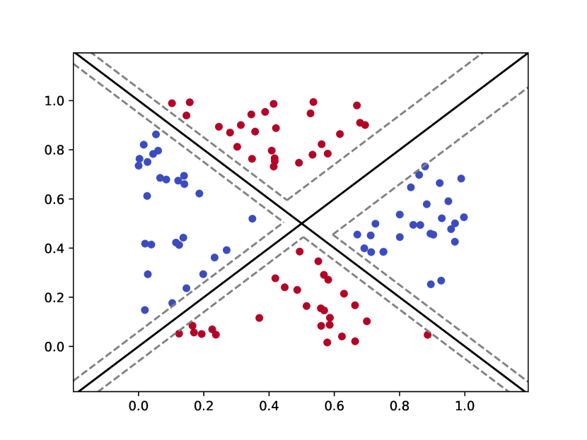
(a) Ground truth

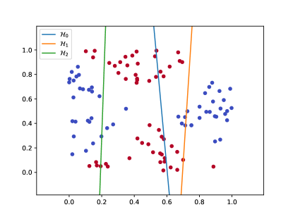
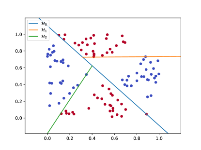
(i) Local SVM Heuristic	(ii) OCT-H

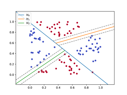
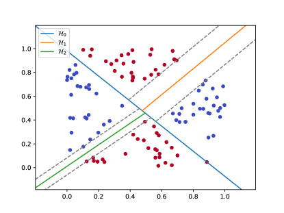
(iii) MM-SVM-OCT	(iv) MARGOT

(b)

Figure 3: Results on the 4-partitions synthetic dataset.

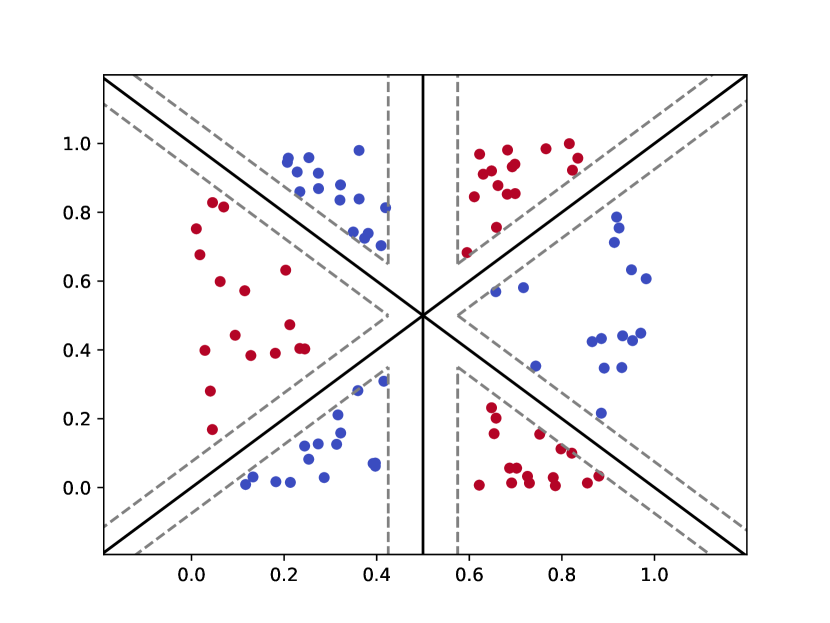
(a) Ground truth

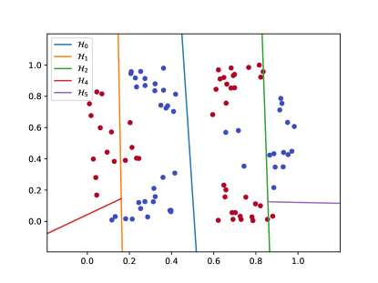
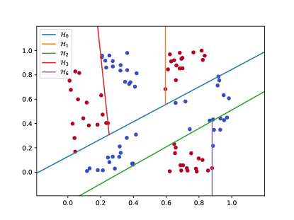
(i) Local SVM Heuristic	(ii) OCT-H

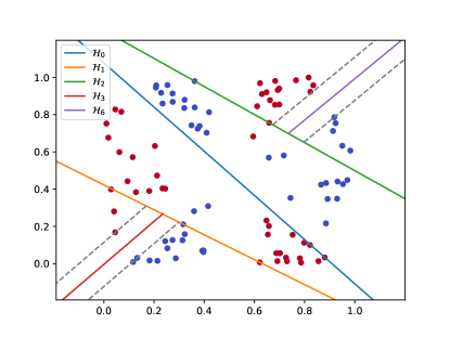
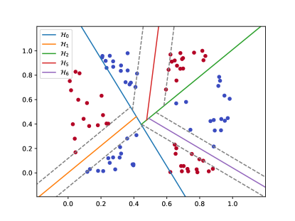
(iii) MM-SVM-OCT	(iv) MARGOT

(b)

Figure 4: Results on the 6-partitions synthetic dataset.

For the 4-partitions dataset, we consider trees with depth $D=2$. Fig. 3(b) (i) represents the tree obtained by the Local SVM Heuristic. Hyperplane $\mathcal{H}_{0}$ at the root node coloured in blue is obtained on the whole dataset, while the hyperplanes at its child nodes, $\mathcal{H}_{1}$ in green and $\mathcal{H}_{2}$ in orange, are obtained considering the partition of the points given by $\mathcal{H}_{0}$ as the splitting rule on the whole dataset. The heuristic returns a classification tree that does not classify all data points correctly, obtaining an accuracy of $86.1\%$. Concerning the OCT approaches in Fig. 3(b) (ii), (iii), and (iv), the solver certified the optimal solution on all three models, thus obtaining 0% MIP gap in different computational times. All three OCT models reach an accuracy of $100\%$. We note that OCT-H creates hyperplanes that do not consider the margin. Indeed, the objective of this approach is to minimize the misclassification cost and the number of features used across the whole tree. Thus, as it happens for the orange hyperplane $\mathcal{H}_{1}$, OCT-H tends to select axis-aligned hyperplanes to split the points. As regards the tree produced by the MM-SVM-OCT model, only the minimum margin among all the hyperplanes is maximized. Consequently, only the green hyperplane $\mathcal{H}_{2}$ lies in the centre between the partitions of points, while the others do not. Instead, the MARGOT tree is the one that most resembles the ground truth in Fig. 3(a) and both the $\mathcal{H}_{1}$ and $\mathcal{H}_{2}$ hyperplanes have a wider margin.

Fig. 4 shows the more complex synthetic dataset 6-partitions where we set $D=3$, the minimum depth to correctly classify all samples. MARGOT and OCT-H reach perfect classification on the whole dataset, and both Local SVM Heuristic and MM-SVM-OCT return good accuracies above 90%. Moreover, the solutions produced by MARGOT and MM-SVM-OCT models are optimal, while OCT-H optimization reaches the time limit with a MIP gap of 50%. In this case as well, MARGOT appears to produce the most reliable classifier among all the generated trees, as it is the one closest to the ground truth.

Finally, we evaluated the four methods on the fourclass dataset. In this case, being the problem the most complex of the three, none of the models has been solved to certified optimality, and OCT-H, MM-SVM-OCT and MARGOT optimization procedures reach a MIP gap of 100%, 74.5% and 67.2% respectively. MARGOT and OCT-H approaches were able to correctly classify almost all the samples, outperforming MM-SVM-OCT, which reaches an accuracy of 88.4%. It is possible to observe how the greedy fashion of the Local SVM Heuristic may generate models not able to capture the underlying truth of the data. Indeed, when applying local SVMs after the split at the root node, it might happen that producing splits is not ”convenient” in terms of the objective function. This is due to the highly nonlinear separability of the dataset, which cannot be effectively handled by a single linear SVM. Thus, when applying the Local SVM Heuristic, not all the possible 15 splits are generated. This case illustrates the drawbacks of the greedy methods compared to optimal ones: when applied to highly non-linearly separable datasets, these heuristic approaches lead to myopic decisions resulting in poor predictive performances.

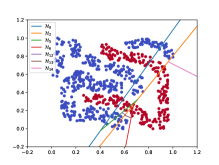
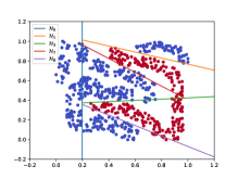
(i) Local SVM Heuristic		(ii) OCT-H

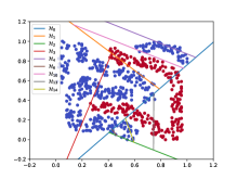
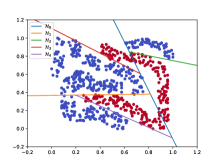
(iii) MM-SVM-OCT		(iv) MARGOT

Figure 5: Results on the fourclass synthetic dataset.

It is worth noticing that all the approaches on the 6-partitions and fourclass datasets tend to minimize the complexity of the tree, i.e. the number of hyperplane splits created. In OCT-H model, this is a consequence of both the penalization of the selection of features in the objective function and the presence of specific constraints and variables which model the pruning of the tree. Similarly, MM-SVM-OCT controls the complexity of the tree with a penalization term in the objective function by introducing binary variables and related constraints. On the contrary, in MARGOT model the complexity is implicitly minimized in the objective function. Indeed, creating an hyperplane split at a node $t$ leads to new coefficients $w_{t}\neq 0$ and variables $\xi_{t}\neq 0$ that appear in the objective function.

				Local SVM				OCT-H				MM-SVM-OCT				MARGOT
Dataset	$|\mathcal{I}|$	$D$		Time	Gap	ACC		Time	Gap	ACC		Time	Gap	ACC		Time	Gap	ACC
4-partitions	108	2		0.1	-	86.1		53.5	0	100		5.2	0	100		0.2	0	100
6-partitions	96	3		0.1	-	91.7		14400	50	100		181.2	0	96.9		4215.0	0	100
fourclass	689	4		126.0	-	80.0		14400	100.0	97.8		14400	74.5	88.4		14400	67.2	99.6

Table 3: Time (s), Gap (%) and ACC (%) performances on the synthetic datasets (time limit $=14400$s $=4$h).

6.2 Results on UCI datasets

We compare the different OCT models computing two predictive measures: the accuracy (ACC) and the balanced accuracy (BACC). The ACC is the percentage of correctly classified samples, and the BACC is the mean of the percentage of correctly classified samples with positive labels and the percentage of correctly classified samples with negative labels.

Hence,

$$ACC=\frac{TP+TN}{TP+TN+FP+FN},$$

$$BACC=\frac{\frac{TP}{TP+FN}+\frac{TN}{TN+FP}}{2},$$

where TP are true positives, TN are true negatives, FP false positives and FN false negatives. Information about the datasets considered is provided in Table 4. We first partitioned each dataset in training ($80\%$) and test ($20\%$) sets and then performed a 4-fold cross-validation (4-FCV) on the training set in order to find the best hyperparameters. In the first set of results where feature selection is not taken into account, the selected hyperparameters are the ones which gave the best average validation accuracy in the cross-validation process. For the second set of results, we implemented a more specific tuning of the hyperparameters to address the sparsity of the hyperplanes’ coefficients, as will be explained later in this section. Once the best hyperparameters are selected, we compute the predictive measures on the training and test sets. The results on the training dataset, as well as all the hyperparameters used in this paper, can be found in the B.

Dataset		$|\mathcal{I}|$	$n$	Class (%)
Breast Cancer D.		569	30	63/36
Breast Cancer W.		683	9	65/35
Climate Model		540	18	9/91
Heart Disease C.		297	13	54/46
Ionosphere		351	34	36/64
Parkinsons		195	22	25/75
Sonar		208	60	53/47
SPECTF H.		267	44	21/79
Tic-Tac-Toe		958	27	35/65
Wholesale		440	7	81/19

Table 4: Information about the datasets considered.

For the resolution of MARGOT, HFS-MARGOT and SFS-MARGOT models, we injected warm start solutions produced by the Local SVM Heuristic. Similarly, for OCT-1, we used as a heuristic solution the one produced by CART [16] using the same setting of OCT-1 for depth $D$, the minimum number of samples per leaf $N_{min}$ and complexity parameter $\alpha$. OCT-H was also given its starting solution, following the warm start procedure presented in [6]. A time limit of 30 seconds was set for every warm start procedure, and an overall time limit of 600 seconds was set for training the models. The maximum depth of the trees generated was fixed to $D=2$, and the ranges of the hyperparameters used in the 4-FCV for the different models are the following:

• For OCT-1 and OCT-H, $N_{min}$ was set to 5% of the total number of training samples and the grid used for the hyperparameter $\alpha$ is $\{0\}\cup\{2^{i}:i\in\{-8,\dots,2\}\}$.

• For MM-SVM-OCT, we used the same grid as the one specified in the related paper; $c_{1}\in\{10^{i}:i\in\{-5,\dots,5\}\}$ and the complexity hyperparameter $c_{3}\in\{10^{i}:i\in\{-2,\dots,2\}\}$.

• For MARGOT, we consider all possible combinations resulting from $C_{t}\in\{10^{i}:i\in\{-5,\dots,5\}\}$ for all $t\in\mathcal{T}_{B}$, and $C_{1}=C_{2}$, imposing the same $C_{t}$ values for all nodes $t$ belonging to the same branching level.

• For HFS-MARGOT, we used the same grid for the $C_{t}$ values as in MARGOT and, concerning the budget parameters $\{B_{t},\text{ for all }t\in\mathcal{T}_{B}\}$, we varied all possible combinations resulting from values of $B_{t}\in\{1,2,3\}$, with $t\in\mathcal{T}_{B}$, considering only combinations where $B_{0}\leq B_{1}=B_{2}$, with the value 3 regarded as the maximum number of features a node can admit in order to be interpretable.

• For SFS-MARGOT, the grid used for the hyperparameter $\alpha$ is $\{2^{i}:i\in\{0,\dots,10\}\}$ and we varied $C_{t}$ values as in MARGOT but in a smaller grid $\{10^{i}:i\in\{-4,-2,0,2,4\}\}$. We set all budget values $B_{t}=1$ for all $t\in\mathcal{T}_{B}$, allowing the model to have full flexibility on where to use more features than the budget value.

6.2.1 Choice of the Big-M and $\varepsilon$

Regarding the $\varepsilon$ parameter used in our formulation, for similar reasons as the one stated in [6], we set $\varepsilon=0.001$ as a compromise between choosing small values that lead to numerical issues and large values that can affect the feasible region excluding possible solutions. Moreover, we carefully tuned the big-M parameters through extensive computational experiments in order to find values as tight as possible. As a result, we set those values as follows:

$$M_{\xi}=M_{w}=50,\ M_{\mathcal{H}}=100,$$

while the Big-M values in MM-SVM-OCT are fixed as indicated in [9].

6.2.2 First set of results

The first set of results is shown in Table 5, where we compare the predictive performances of MARGOT against OCT-H and MM-SVM-OCT. We can see how MARGOT takes full advantage of the generalization capabilities deriving from the maximum margin approach, resulting in much higher ACC and BACC scores on the test sets.

		OCT-H			MM-SVM-OCT			MARGOT
Dataset		ACC	BACC		ACC	BACC		ACC	BACC
Breast Cancer D.		94.7	94.3		93.9	92.7		97.4	96.9
Breast Cancer W.		94.9	95.6		96.4	96.2		96.4	96.2
Climate Model		93.5	86.4		97.2	88.4		97.2	88.4
Heart Disease C.		80.0	79.7		81.7	81.3		83.3	83.0
Ionosphere		87.3	85.7		85.9	80.9		93.0	90.0
Parkinsons		82.1	84.7		87.2	81.6		84.6	83.1
Sonar		66.7	65.9		73.8	73.0		73.8	73.0
SPECTF H.		74.1	53.3		79.6	50.0		79.6	56.8
Tic-Tac-Toe		96.9	96.2		97.4	97.0		97.9	97.0
Wholesale		84.1	79.8		83.0	74.2		87.5	85.1

Table 5: Results on the test predictive performances of the OCT models evaluated: test ACC (%) and test BACC (%).

Computational times and MIP gaps can be found in Table 6. It is clear how MARGOT optimization problem is much easier to solve than OCT-H and MM-SVM-OCT. Indeed, 9 times out of 10, MARGOT reaches the optimal solution with a mean computational time and MIP gap of 121.5 seconds and 0.3%, respectively. MM-SVM-OCT reaches the optimal solution 3 times out of 10, with a mean running time and gap of 482.7 seconds and 18.8% respectively, and OCT-H reaches the optimum only in one case, with a mean time and gap of 564.3 seconds and 63.7% respectively.

		OCT-H			MM-SVM-OCT			MARGOT
Dataset		Time	Gap		Time	Gap		Time	Gap
Breast Cancer D.		620.2	72.8		600.2	27.5		7.4	0.0
Breast Cancer W.		615.3	80.1		333.0	0.0		8.7	0.0
Climate Model		620.2	90.6		600.2	0.6		10.7	0.0
Heart Disease C.		630.1	91.9		600.0	28.8		318.1	0.0
Ionosphere		59.1	0.0		600.0	8.4		11.2	0.0
Parkinsons		612.3	90.8		600.1	12.5		207.4	0.0
Sonar		620.2	96.1		262.7	0.0		1.5	0.0
SPECTF H.		620.2	96.9		30.3	0.0		600.2	3.3
Tic-Tac-Toe		625.4	100.0		600.1	78.1		3.5	0.0
Wholesale		620.1	95.6		600.0	32.4		46.4	0.0

Table 6: Results on the optimization performances of the OCT models evaluated: computational times (s) and MIP Gaps (%).

6.2.3 Second set of results: feature selection

In the following set of results, we compare HFS-MARGOT and SFS-MARGOT with OCT-1 and OCT-H. Both MARGOT and MM-SVM-OCT do not appear in this set of results because these models do not address the sparsity of the hyperplanes’ weights. For this analysis, a different hyperparameter selection was carried out. This was done to take into account that we are not just comparing the predictive performances of the methods, but we are also evaluating the feature selection aspect. The 4-FCV was still conducted, but this time we did not select the hyperparameters which gave the highest mean validation accuracy. Indeed, the highest mean validation accuracy values yield to models which select a high number of features, thus contrasting the aim to create more interpretable trees. At the same time, solely considering sparsity is not useful as the hyperparameters which gave the best results in terms of feature selection may result in less performing classifiers.

		OCT-1			OCT-H*			HFS-MARGOT*			SFS-MARGOT*
Dataset		ACC	BACC		ACC	BACC		ACC	BACC		ACC	BACC
Breast Cancer D.		91.2	91.6		94.7	94.3		95.6	95.5		94.7	94.3
Breast Cancer W.		92.0	90.9		92.0	91.4		94.2	94.5		94.2	93.6
Climate Model		91.7	60.1		98.1	93.9		96.3	77.8		96.3	82.8
Heart Disease C.		71.7	71.0		80.0	79.5		83.3	82.6		86.7	86.2
Ionosphere		91.5	91.7		90.1	86.9		87.3	83.8		84.5	79.8
Parkinsons		89.7	83.3		87.2	81.6		89.7	83.3		87.2	84.8
Sonar		69.0	68.9		71.4	71.1		71.4	70.9		73.8	73.6
SPECTF H.		77.8	65.8		75.9	51.1		75.9	57.8		83.3	65.9
Tic-Tac-Toe		69.3	61.5		96.4	95.5		76.0	65.7		97.9	97.0
Wholesale		86.4	85.2		87.5	86.1		86.4	85.2		88.6	86.9

Table 7: Results on the test predictive performances of the OCT models with feature selection: test ACC (%) and test BACC (%).

		OCT-1			OCT-H*			HFS-MARGOT*			SFS-MARGOT*
Dataset		Time	Gap		Time	Gap		Time	Gap		Time	Gap
Breast Cancer D.		600.0	96.3		620.2	72.8		313.9	0.0		314.7	0.0
Breast Cancer W.		138.6	0.0		615.4	72.3		14.1	0.0		37.6	0.0
Climate Model		600.0	100.0		620.1	81.4		600.3	100.0		600.4	14.2
Heart Disease C.		93.3	0.0		630.1	86.9		106.5	0.0		600.3	28.2
Ionosphere		600.0	52.0		625.2	83.2		124.0	0.0		15.9	0.0
Parkinsons		600.0	92.9		620.1	82.4		7.8	0.0		600.2	62.0
Sonar		600.1	30.7		620.1	91.4		601.2	98.3		610.8	42.2
SPECTF H.		600.0	98.0		626.1	94.5		601.3	93.8		610.1	99.9
Tic-Tac-Toe		268.1	0.0		630.0	94.7		604.6	88.2		47.2	0.0
Wholesale		600.0	86.5		620.2	73.5		36.4	0.0		600.2	80.1

Table 8: Results on the optimization performances of the OCT models with feature selection: computational times (s) and MIP Gap values (%).

Thus, we proceeded as follows. For each dataset, after performing the standard 4-FCV, we highlighted the combinations of hyperparameters which resulted in a mean validation accuracy in the range $[0.975\gamma,\gamma]$, where $\gamma$ is the best mean validation accuracy value scored. This way, we selected the combinations of hyperparameters corresponding to ”good” classifiers. Among these combinations, we chose the ones corresponding to the lower number of features used, and, among these last ones, we picked the combination corresponding to the best validation accuracy. We denote by OCT-H*, HFS-MARGOT* and SFS-MARGOT* the tree models generated with this feature selection driven hyperparameter tuning. For OCT-1, we performed the standard hyperparameter search considering that the univariate splits of the model are sparse by definition. To the best of our knowledge, this is the first time a tailored cross-validation was carried out to fairly compare optimization-based ML models that embed feature selection.

Tables 7 and 8 report both the predictive and optimization performances of the compared models. Tables 9 and 10, together with their graphical representation in Figure 6, show the difference in the features selected among the analysed OCT models. We denote by $F$ the set of distinct features used overall in the tree, and by $F_{t}$ the set of features selected at node $t$. As expected, MARGOT and MM-SVM-OCT models tend to use all the available features because they have no feature selection constraints or penalization terms in the objective function. One thing to notice is that, in many cases, MM-SVM-OCT tends to activate more branch splits than MARGOT, each involving all the features. This might be due to the difference in the objective functions of the two models. Moreover, the OCT-H model for which a standard 4-FCV is carried out, tends to produce sparser tree models since the number of features selected is penalized in its formulation.

OCT-1, OCT-H*, HFS-MARGOT* and SFS-MARGOT* generate models selecting a lower number of features, maintaining good prediction performances, as shown in Table 7. In particular, we can notice how SFS-MARGOT* presents better ACC and BACC values, and this is probably due to the combination of the maximum margin approach and the feature selection penalization. Indeed, we can see how SFS-MARGOT*, where violation of the budget constraints is allowed, has more freedom in the selection of features compared to the more restrictive approach of HFS-MARGOT*, which at each node cannot exceed a predefined number of selected features. One thing to notice is that, on these results, both OCT-H and OCT-H* tend to use the selected features just in the first branch node of the tree. A similar behaviour is exhibited by the SFS-MARGOT^∗ model. In contrast, the features selected by HFS-MARGOT^∗ tend to be more spread throughout the branch nodes. Using hard budget constraints limiting the number of features selected at each branch node has indeed two consequences: on the one hand, it spreads more evenly the features selected among the tree structure, while on the other, this restriction might result insufficient in order achieve the best performances. This is the case of the Tic-Tac-Toe dataset where the HFS-MARGOT* model clearly did not perform well, and this is most likely because the values we adopted for budget parameters $B_{t}$ were too limiting. In this sense, OCT-1 represents the extreme case, in that it is limited to select only one feature per split, generally worsening the predictive quality of the classifier. Of course, for HFS-MARGOT*, we could have used higher budget values, but this, apart from leading to less interpretable tree structures and time-consuming hyperparameters tuning, does not attain the scope of our computational results. We finally note how OCT-1 is easier to solve than OCT-H*, closing the gap in 3 datasets, but it still results to be computationally more expensive than the MARGOT feature selection models.

In Figures 8, we give more insight into how the features selected by the different OCT models divide the training samples. We focused on two datasets, the Parkinsons and the Breast Cancer D. ones, in that we found them explicative of the behaviour of all the trees generated by OCT-1, OCT-H*, HFS-MARGOT* and SFS-MARGOT* models.

			OCT-H			MM-SVM-OCT			MARGOT
Dataset	$n$		$|F|$	$|F_{0}|,|F_{1}|,|F_{2}|$		$|F|$	$|F_{0}|,|F_{1}|,|F_{2}|$		$|F|$	$|F_{0}|,|F_{1}|,|F_{2}|$
Breast Cancer D.	30		3	3, 0, 0		30	30, 30, 30		30	30, 30, 0
Breast Cancer W.	9		4	4, 0, 0		9	9, 9, 0		9	9, 8, 0
Climate Model	18		11	11, 0, 0		18	18, 18, 18		18	18, 0, 18
Heart Disease C.	13		4	4, 0, 0		13	13, 0, 0		13	13, 0, 6
Ionosphere	34		32	28, 22, 23		33	33, 33, 33		33	33, 33, 31
Parkinsons	22		13	7, 0, 8		22	22, 22, 22		22	22, 22, 22
Sonar	60		23	23, 0, 0		60	60, 60, 60		51	51, 0, 0
SPECTF H.	44		25	10, 4, 17		0	0, 0, 0		44	44, 0, 42
Tic-Tac-Toe	27		26	18, 18, 1		27	26, 26, 22		18	18, 0, 0
Wholesale	7		7	6, 0, 5		7	7, 7, 7		7	7, 0, 6

Table 9: Comparison on the number of features selected by the OCT models; $F$ is is the set of features used in the tree, and $F_{t}$ are the features selected at the node $t=0,1,2$.

			OCT-1			OCT-H*			HFS-MARGOT*			SFS-MARGOT*
Dataset	$n$		$|F|$	$|F_{0}|,|F_{1}|,|F_{2}|$		$|F|$	$|F_{0}|,|F_{1}|,|F_{2}|$		$|F|$	$|F_{0}|,|F_{1}|,|F_{2}|$		$|F|$	$|F_{0}|,|F_{1}|,|F_{2}|$
Breast Cancer D.	30		2	1, 0, 1		3	3, 0, 0		4	2, 0, 2		3	3, 0, 0
Breast Cancer W.	9		3	1, 1, 1		2	2, 0, 0		4	2, 3, 0		3	3, 0, 0
Climate Model	18		2	1, 1, 1		7	7, 0, 0		6	3, 3, 0		4	4, 0, 0
Heart Disease C.	13		1	1, 0, 0		3	3, 0, 0		3	1, 2, 2		6	6, 0, 0
Ionosphere	34		2	1, 0, 1		3	2, 0, 1		7	2, 2, 3		2	1, 0, 1
Parkinsons	22		2	1, 1, 1		5	3, 3, 0		3	1, 2, 0		12	9, 2, 4
Sonar	60		1	1, 0, 0		15	15, 0, 0		5	1, 2, 2		8	7, 0, 1
SPECTF H.	44		2	1, 0, 1		5	5, 0, 0		6	2, 1, 3		10	9, 1, 0
Tic-Tac-Toe	27		2	1, 0, 1		18	18, 0, 0		5	2, 3, 0		18	18, 0, 0
Wholesale	7		2	1, 1, 1		2	2, 0, 0		5	1, 2, 2		3	3, 0, 0

Table 10: Comparison on the number of features selected by the OCT models with feature selection; $F$ is is the set of features used in the tree, and $F_{t}$ are the features selected at the node $t=0,1,2$.

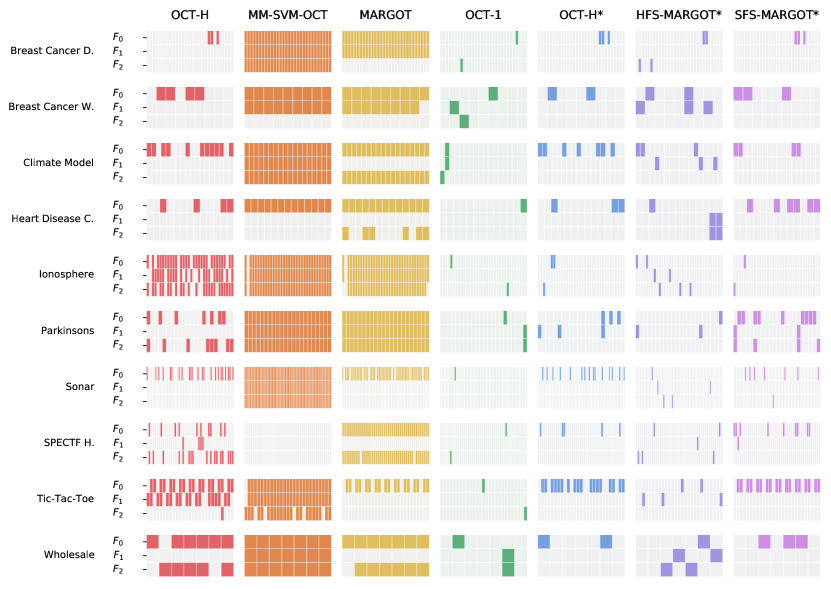
Figure 6: Graphical representation of Tables 9, 10: for each branch node $t$, the darker coloured cells correspond to the features selected $F_{t}$.

OCT-1

OCT-H*

HFS-MARGOT*

SFS-MARGOT*

(a) Parkinsons

OCT-1

OCT-H*

HFS-MARGOT*

SFS-MARGOT*

(b) Breast Cancer D.

Figure 8: Trees generated by models in Table 7 on the Parkinsons and Breast Cancer D. datasets. For each branch node, we report the number of positive and negative training samples in the squared brackets and below the features selected at each node. For each leaf node, the number of positive and negative samples is indicated, together with the assigned class label.

6.3 Warm Start

During the branch and bound process implemented by Gurobi, after finding an initial incumbent solution, the solver applies heuristics to improve the quality of the incumbent solution before further exploring the branch and bound tree. In general, a warm start input solution is accepted as the first incumbent if its value is better than the initial solution found by the solver. In Table 11, we analyse the quality of the warm start input solution produced by the Local SVM Heuristic. To this aim, we introduce the following definitions: $f_{0}$ refers to the value of the first incumbent solution, and $f_{1}$ is the value of the best incumbent solution after the root node of the branch and bound tree has been explored. We report these values in two different cases. In the first one, no input solution was injected, while in the second, the solver was given the warm start computed with the Local SVM Heuristic. From the results in the tables, we can see how generally the value of the Local SVM solution is better than the one of the first incumbent solution found by Gurobi. Only for the SPECTF H. dataset, our warm start for HFS-MARGOT model did not produce a better first solution. Similarly, in most cases, $f_{1}$ values are better when the Local SVM solution is injected. Moreover, we can notice how, almost every time the Local SVM input solution was given, values $f_{0}$ and $f_{1}$ are equal.

MARGOT		$f_{0}$			$f_{1}$
Dataset		No warm start	Local SVM		No warm start	Local SVM
Breast Cancer D.		412.69	71.33		73.31	71.33
Breast Cancer W.		41939.75	5250.53		5357.29	5250.53
Climate Model		2592000000398.93	94.14		113.17	94.14
Heart Disease C.		29.56	18.48		18.48	18.48
Ionosphere		1680000000000.00	768.96		726.56	768.96
Parkinsons		306298.02	196369.04		213242.43	196369.04
Sonar		11.02	11.01		0.17	0.35
SPECTF H.		127800000000.00	17.47		17.47	17.47
Tic-Tac-Toe		346.00	84.00		84.00	84.00
Wholesale		349170.61	104787.61		104787.61	104787.61
HFS-MARGOT		$f_{0}$			$f_{1}$
Dataset		No warm start	Local SVM		No warm start	Local SVM
Breast Cancer D.		569527.09	78042.45		569527.09	78042.45
Breast Cancer W.		45466685.23	7278653.51		45466685.23	7278653.51
Climate Model		7400074.00	6624789.91		7400073.21	6624789.91
Heart Disease C.		107570.28	98193.89		107570.28	98193.89
Ionosphere		2820.49	1477.29		2820.49	1477.29
Parkinsons		119951.06	88203.38		119951.06	88203.38
Sonar		1434.07	990.21		1434.07	990.21
SPECTF H.		0.89	0.89		0.89	0.89
Tic-Tac-Toe		58300.00	46528.00		54822.00	46528.00
Wholesale		7532.43	7256.24		7532.43	7256.24
SFS-MARGOT		$f_{0}$			$f_{1}$
Dataset		No warm start	Local SVM		No warm start	Local SVM
Breast Cancer D.		125004.07	7382.54		24619.24	7382.54
Breast Cancer W.		810.54	117.26		206.87	117.26
Climate Model		61588.84	14800.00		14800.00	14800.00
Heart Disease C.		414.07	215.00		299.28	215.00
Ionosphere		1120000004951.79	247.86		404.00	247.86
Parkinsons		376661.06	194921.43		344525.19	194921.43
Sonar		902.33	228.87		311.75	228.87
SPECTF H.		85200000033077.50	18794.98		8800.01	8800.01
Tic-Tac-Toe		3064000691010.00	101.00		101.00	101.00
Wholesale		40023.52	12177.22		12438.92	12177.22

Table 11: Warm start analysis for MARGOT, HFS-MARGOT and SFS-MARGOT

7 Conclusions and future research

In this paper, we propose a novel MIQP model, MARGOT, to train multivariate optimal classification trees which employ maximum margin hyperplanes by following the soft SVM paradigm. The proposed model presents fewer binary variables and constraints than other OCT methods by exploiting the SVM approach and the binary classification setting, resulting in a much more compact formulation. The computational experience shows that MARGOT results in a much easier model to solve compared to state-of-the-art OCT models, and, thanks to the statistical properties inherited by the SVM approach, it reaches better predictive performances. In the case sparsity of the hyperplane splits is a desirable requirement, HFS-MARGOT and SFS-MARGOT represent two valid interpretable alternatives, which model feature selection with hard budget constraints and soft penalization, respectively. Both the feature selection versions are comparable to OCT-H and MM-SVM-OCT approaches in terms of prediction quality, though they are easier to solve. On the one hand, HFS-MARGOT, results in a more interpretable model where the selected features are evenly spread among tree branch nodes without losing too much prediction quality. On the other, SFS-MARGOT presents better out-of-sample performances than HFS-MARGOT, though the selection of the features does not exploit the hierarchical tree structure of the classifier as much.

Plenty of future directions of this work are of interest. Firstly, the method can be extended to deal with the multi-class case. In addition, being SVMs widely used for regression tasks, a similar version of MARGOT to learn optimal regression trees can be further addressed. Lastly, the development of a tailored optimization algorithm for the resolution of the proposed models can be investigated to improve computational times on real-world instances.

Appendix A Additional results

In this section, we present additional computational results regarding the OCT models.

A.1 Scalability of MARGOT and OCT-H models with respect to the depth

In order to assess how the resolution of MARGOT and OCT-H optimization models scales with increasing depth values, we compare the two models with depths $D\in\{2,3,4\}$. The hyperparameters used are the same as the ones selected for $D=2$ (reported in Table 21) to evaluate how the optimization problems scale only with respect to the depth hyperparameter. The same time limit of $3600$ seconds was set for all experiments, and a time limit of $120$ seconds was set for the warm start procedure. Results on both predictive and computational performances are presented in an aggregated form using box plots 9. We can notice how, regarding the predictive performances, both models perform similarly for every depth value, with a slight decrease at $D=4$. Regarding the computational performances, both optimization models become harder to solve, with OCT-H reaching higher MIP Gap values than MARGOT. We notice that, though not deducible from the boxplots, OCT-H with depths $D\in\{3,4\}$ was able to achieve a MIP Gap value of 0 only for the Ionosphere dataset, while MARGOT with $D=3$ certified the optimal solution only for the Breast Cancer D. and the Sonar datasets, while it always reached the time limit for depth $D=4$. In general, scaling with respect to the depth is a challenging aspect in MIP-based OCT models as they become more complex to solve, presenting a high computational complexity depending both on the data dimensionality and on the depth of the tree. In particular, as shown in Table 1, in MARGOT, both variables and constraints grow exponentially with the depth $D$ of the tree, and the same can be stated for OCT-H ([6]). Nonetheless, solving MARGOT for increasing values of $D$ seems to be more tractable than solving OCT-H.

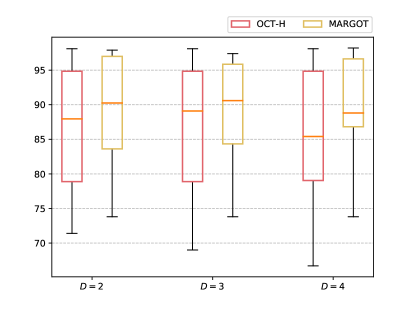
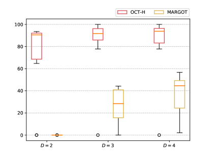
Test ACC (%)	MIP Gap (%)

Figure 9: Aggregated representation of the Test ACC (%) and MIP Gap (%) values of OCT-H and MARGOT model with depths $D\in\{2,3,4\}$.

A.2 Comparison of HFS-MARGOT against univariate optimal trees with higher depths

In the following analysis, we compare HFS-MARGOT* with $D=2$ against the univariate model OCT-1 with $D\in\{2,3,4\}$ in order to assess if employing shallow and sparse multivariate trees ultimately pays off even if univariate ones are allowed higher depths. In general, multivariate splits are less interpretable but allow for more flexibility, yielding shallow trees with less branching levels than univariate ones. In this comparison, we consider only HFS-MARGOT* in that it represents the most sparse multivariate MARGOT model. Thus, if in this extreme case, HFS-MARGOT* performs better, we can deduce that MARGOT and SFS-MARGOT* will perform similarly, if not much better, in terms of predictive capabilities, but at the expense of interpretability.

For OCT-1 with $D\in\{3,4\}$, we maintained the same values of $\alpha$ and $N_{min}$ chosen for OCT-1 with $D=2$. We set a time limit of $1800$ and $3600$ seconds for $D=3$ and $D=4$ respectively. For the computation of the warm start solutions, the time limit was set to $60$ and $120$ seconds for the two depth values, respectively. Table 12 reports the predictive test performances and the number of all the (non-distinct) features used computed as $\sum_{t\in\mathcal{T}_{B}}|F_{t}|$. Moreover, the mean MIP Gap value and its standard deviation are provided for each model evaluated. We can notice how HFS-MARGOT* with a shallow depth of 2 favourably compares to OCT-1 in terms of prediction quality even in the case where the latter is allowed a depth of 4, sometimes even using far fewer features. It is also evident that OCT-1 struggles to scale efficiently to higher depths, showing larger mean gaps even if provided with higher time limit values. Though not explicitly deducible in the table, we highlight that for OCT-1 with depths $D=\{3,4\}$, the solver never certified the optimal solution except for just a single dataset (Heart Disease C). The train predictive performances are reported in Table 20.

		OCT-1 ($D=2$)				OCT-1 ($D=3$)				OCT-1 ($D=4$)				HFS-MARGOT* ($D=2$)
Dataset		ACC	BACC	$\sum|F_{t}|$		ACC	BACC	$\sum|F_{t}|$		ACC	BACC	$\sum|F_{t}|$		ACC	BACC	$\sum|F_{t}|$
Breast Cancer D.		91.2	91.6	2		94.7	94.3	3		95.6	95.5	4		95.6	95.5	4
Breast Cancer W.		92.0	90.9	3		92.7	92.0	6		92.7	92.5	11		94.2	94.5	5
Climate Model		91.7	60.1	3		91.7	60.1	6		93.5	76.3	15		96.3	77.8	6
Heart Disease C.		71.7	71.0	1		71.7	71.0	1		71.7	71.0	1		83.3	82.6	5
Ionosphere		91.5	91.7	2		93.0	92.7	2		93.0	92.7	2		87.3	83.8	7
Parkinsons		89.7	83.3	3		82.1	81.4	7		92.3	91.6	15		89.7	83.3	3
Sonar		69.0	68.9	1		61.9	61.8	1		69.0	68.9	1		71.4	70.9	5
SPECTF H.		77.8	65.8	2		83.3	69.2	3		79.6	63.5	6		75.9	57.8	6
Tic-Tac-Toe		69.3	61.5	2		74.5	63.4	3		72.9	65.0	5		76.0	65.7	5
Wholesale		86.4	85.2	3		85.2	83.5	2		84.1	82.6	4		86.4	85.2	5
Mean Gap		55.6 ($\pm$ 44.3)				75.7 ($\pm$ 36.5)				77.9 ($\pm$ 35.6)				38.0 ($\pm$ 49.2)

Table 12: Results on the test predictive performances (test ACC (%) and test BACC (%)) of OCT-1 model with $D\in\{2,3,4\}$ and HFS-MARGOT* model with $D=2$ and comparison on the number of (non-distinct) features used $\sum_{t\in\mathcal{T}_{B}}|F_{t}|$. The last row is the Mean MIP Gap values ($\pm$ standard deviations) (%) among all datasets for each model.

A.3 Results with a fixed set of hyperparameters

Here we provide a set of experiments on MARGOT, HFS-MARGOT and SFS-MARGOT, with depth $D=2$, using a fixed set of hyperparameters across all datasets. The time limit was set to $600$ seconds, while the warm start optimization was given a limit of $30$ seconds. These experiments allow us to evaluate the robustness of the proposed methods without conducting an ad-hoc hyperparameter search for each dataset. We have chosen a set of hyperparameters that was never selected by the 4-FCV and that could be considered a reasonable choice. The fixed set of hyperparameters chosen for the MARGOT models is reported in Table 13.

Tables 14, 15, 16 provide the predictive and optimization performances obtained with the fixed set of hyperparameters. For each performance measure (ACC, BACC, Time or Gap), we provide the difference $d$ defined as:

$$d=\pm\left|\text{best value - actual value}\right|,$$

where the best value is the value of the performance measure obtained using the hyperparameters in Tables 21 and 22 obtained with the 4-FCV, whereas actual value is the value obtained with the hyperparameters set as in Table 13. The sign is ”$+$” when the best value obtained by 4-FCV is better, otherwise it is ”$-$”. Table 14 reports the predictive performances on the test sets. These results show that, despite using the same set of hyperparameters, all the methods achieve good generalization performances across all the datasets. Additionally, Table 16 provides the computational times and MIP Gap values. It is evident that the MARGOT model is easier to solve, certifying the optimal solutions in 8 out of 10 datasets. Performances on the train sets can be found in Table 15, where it is possible to notice that MARGOT and SFS-MARGOT tend to overfit on some datasets. This result was expected in that, without conducting a cross-validation procedure, the risk of overfitting is higher. Overall, these results show that MARGOT models are robust, reporting overall good prediction quality, without the need for a dataset-specific hyperparameter search. However, a tailored hyperparameter tuning can be advisable to mitigate the risk of overfitting and to maximize the model’s potential.

MARGOT

HFS-MARGOT

SFS-MARGOT

Dataset

$C_{0}$

$C_{1}=C_{2}$

$C_{0}$

$C_{1}=C_{2}$

$B_{0}$

$B_{1}=B_{2}$

$C_{0}$

$C_{1}=C_{2}$

$\alpha$

all

$10^{2}$

$10^{3}$

$10^{2}$

$10^{3}$

2

2

$10^{2}$

$10^{3}$

$2^{5}$

Table 13: Hyperparameters selected for results in Table 14, Table 15 and Table 16.

		MARGOT				HFS-MARGOT				SFS-MARGOT
Dataset		ACC	BACC	$d$		ACC	BACC	$d$		ACC	BACC	$d$
Breast Cancer D.		94.7	94.3	2.6 / 2.6		95.6	95.5	0.0 / 0.0		95.6	94.5	-0.9 / -0.2
Breast Cancer W.		93.4	93.0	2.9 / 3.2		93.4	93.5	0.7 / 1.0		93.4	93.0	0.7 / 0.6
Climate Model		94.4	81.8	2.8 / 6.6		92.6	65.7	3.7 / 12.1		95.4	87.4	0.9 / -4.5
Heart Disease C.		81.7	81.7	1.7 / 1.3		73.3	72.3	10.0 / 10.3		83.3	83.3	3.3 / 2.9
Ionosphere		87.3	83.8	5.6 / 6.2		85.9	81.8	1.4 / 2.0		83.1	78.7	1.4 / 1.1
Parkinsons		89.7	93.1	-5.1 / -10.0		87.2	81.6	2.6 / 1.7		92.3	94.8	-5.1 / -10.0
Sonar		73.8	73.0	0.0 / 0.0		69.0	68.9	2.4 / 2.0		76.2	75.5	-2.4 / -1.8
SPECTF H.		75.9	61.2	3.7 / -4.4		79.6	60.1	-3.7 / -2.3		74.1	56.7	9.3 / 9.2
Tic-Tac-Toe		95.3	95.4	4.7 / 2.4		70.3	62.0	5.7 / 3.7		96.4	95.8	1.6 / 1.2
Wholesale		87.5	85.1	0.0 / 0.0		88.6	86.9	-2.3 / -1.7		87.5	85.1	1.1 / 1.8
Mean		87.4	84.2	1.9 / 0.8		83.6	76.8	2.1 / 2.9		87.7	84.5	1.0 / 0.0

Table 14: Results on the predictive test performances (test ACC (%) and test BACC (%)) of MARGOT models with $D=2$ and the hyperparameters set as in Table 13 and difference $d=\pm|\text{best value - actual value}|$; a value $d>0$ indicates an advantage for 4-FCV selection, while $d<0$ denotes an advantage for the fixed set of hyperparameters.

		MARGOT				HFS-MARGOT				SFS-MARGOT
Dataset		ACC	BACC	$d$		ACC	BACC	$d$		ACC	BACC	$d$
Breast Cancer D.		100.0	100.0	-0.7 / -0.9		98.0	97.4	0.0 / 0.0		100.0	100.0	-1.8 / -2.2
Breast Cancer W.		100.0	100.0	-1.1 / -0.9		97.6	97.7	0.7 / 0.9		100.0	100.0	-2.2 / -2.4
Climate Model		100.0	100.0	-0.7 / -4.1		95.1	74.1	1.6 / 7.0		100.0	100.0	-3.2 / -15.2
Heart Disease C.		93.7	93.6	-4.6 / -4.7		83.5	83.0	-0.8 / -0.9		89.5	89.4	-3.0 / -3.3
Ionosphere		100.0	100.0	-1.1 / -1.3		92.5	90.5	1.4 / 1.8		100.0	100.0	-9.6 / -12.9
Parkinsons		100.0	100.0	0.0 / 0.0		92.3	86.0	-1.3 / -3.5		100.0	100.0	0.0 / 0.0
Sonar		100.0	100.0	0.0 / 0.0		85.5	85.3	-6.6 / -7.1		100.0	100.0	-9.0 / -9.7
SPECTF H.		100.0	100.0	-3.3 / -8.0		86.9	75.7	-1.9 / -1.2		100.0	100.0	-8.9 / -19.1
Tic-Tac-Toe		100.0	100.0	-1.6 / -2.3		72.6	64.6	5.5 / 3.7		100.0	100.0	-1.6 / -2.3
Wholesale		96.3	95.2	0.0 / 0.0		93.8	93.3	0.0 / 1.4		96.3	95.2	-1.1 / -0.6
Mean		99.0	98.9	-1.3 / -2.2		89.8	84.8	-0.1 / 0.2		98.6	98.5	-4.0 / -6.8

Table 15: Results on the predictive train performances (train ACC (%) and train BACC (%)) of MARGOT models with $D=2$ and the hyperparameters set as in Table 13 and difference $d=\pm|\text{best value - actual value}|$; a value $d>0$ indicates an advantage for 4-FCV selection, while $d<0$ denotes an advantage for the fixed set of hyperparameters.

		MARGOT				HFS-MARGOT				SFS-MARGOT
Dataset		Time	Gap	$d$		Time	Gap	$d$		Time	Gap	$d$
Breast Cancer D.		3.9	0.0	-3.5 / 0.0		600.8	79.6	286.9 / 79.6		608.0	11.1	293.4 / 11.1
Breast Cancer W.		149.2	0.0	140.5 / 0.0		126.1	0.0	112.1 / 0.0		451.9	0.0	414.3 / 0.0
Climate Model		10.5	0.0	-0.2 / 0.0		600.2	78.6	-0.1 / -21.4		600.3	3.7	0.2 / -10.5
Heart Disease C.		600.0	81.2	281.9 / 81.2		600.2	80.3	493.7 / 80.3		600.2	83.5	0.2 / 55.2
Ionosphere		13.3	0.0	2.1 / 0.0		600.8	85.1	476.8 / 85.1		601.8	24.1	585.8 / 24.1
Parkinsons		3.0	0.0	-204.4 / 0.0		600.4	74.1	592.2 / 74.1		600.6	4.4	0.6 / -57.6
Sonar		0.2	0.0	-1.4 / 0.0		602.7	91.2	1.8 / -7.1		620.1	4.9	20.1 / -37.3
SPECTF H.		10.2	0.0	-590.0 / -3.3		600.8	88.7	0.8 / -5.1		615.7	20.8	15.6 / -79.1
Tic-Tac-Toe		172.8	0.0	169.3 / 0.0		602.5	90.1	2.4 / 1.9		604.3	14.8	557.1 / 14.8
Wholesale		600.0	31.6	553.6 / 31.6		600.1	22.1	563.8 / 22.1		600.1	31.6	0.1 / -48.5
Mean		156.3	11.3	34.8 / 11.0		553.5	69.0	253.1 / 30.9		590.3	19.9	188.7 / -12.8

Table 16: Results on the optimization performances (computational times (s) and MIP Gaps (%)) of MARGOT models with $D=2$ and the hyperparameters set as in Table 13 and difference $d=\pm|\text{best value - actual value}|$; a value $d>0$ indicates an advantage for 4-FCV selection, while $d<0$ denotes an advantage for the fixed set of hyperparameters.

Appendix B Additional tables

In this section, we present additional tables. Table 17 presents a summary of all the notation of sets, parameters, and hyperparameters adopted in the paper. ACC and BACC performances on training samples are reported in Tables 18, 19 and 20. Finally, for the sake of replicability, we present in Tables 21 and 22 all the hyperparameters that were chosen to carry out our computational experiments.

Notation		Description
Sets
$\mathcal{T}_{B}$		Branch nodes
$\mathcal{T}_{L}$		Leaf nodes
$\mathcal{T}_{B}^{\prime}$		Branch nodes excluded the ones in the last branching level
$\mathcal{T}_{B}^{\prime\prime}$		Branch nodes of the last branching level
$\mathcal{S}(t)$		Branch nodes of the subtree rooted at node $t\in\mathcal{T}_{B}$
$\mathcal{S}^{\prime\prime}(t)$		Nodes of $\mathcal{S}(t)$ in the last branching level $\mathcal{T}_{B}^{\prime\prime}$
$\mathcal{S}^{\prime\prime}_{L}(t)$		Nodes in $\mathcal{T}_{B}^{\prime\prime}$ under the left branch of $t\in\mathcal{T}_{B}^{\prime}$
$\mathcal{S}^{\prime\prime}_{R}(t)$		Nodes in $\mathcal{T}_{B}^{\prime\prime}$ under the right branch of $t\in\mathcal{T}_{B}^{\prime}$
$\mathcal{I}$		Index set of data samples
$\mathcal{I}_{t}$		Index set of data samples assigned to node $t\in\mathcal{T}_{B}$
$\mathcal{I}_{L(t)}$		Index set of data samples assigned to the left child node of $t\in\mathcal{T}_{B}$
$\mathcal{I}_{R(t)}$		Index set of data samples assigned to the right child node of $t\in\mathcal{T}_{B}$
Parameters
$n$		Number of features
$\varepsilon$		Parameter to model the strict inequality in routing constraints
$\{M_{w},M_{\xi},M_{\mathcal{H}}\}$		Set of Big-M parameters used in MARGOT formulations
Hyperparameters
$D$		Maximum depth of the tree
$C_{t}$		Penalty parameter on the misclassification error at node $t\in\mathcal{T}_{B}$
$B_{t}$		Budget value on the number of features at node $t\in\mathcal{T}_{B}$
$\alpha$		Penalty parameter for the soft feature selection

Table 17: Notation: sets, parameters and hyperparameters of MARGOT models.

		OCT-H			MM-SVM-OCT			MARGOT
Dataset		ACC	BACC		ACC	BACC		ACC	BACC
Breast Cancer D.		98.2	97.8		98.7	98.2		99.3	99.1
Breast Cancer W.		98.4	98.6		98.2	98.0		98.9	99.2
Climate Model		98.6	91.9		99.3	95.9		99.3	95.9
Heart Disease C.		85.7	85.6		88.6	88.5		89.0	88.9
Ionosphere		100.0	100.0		98.6	98.2		98.9	98.7
Parkinsons		99.4	98.7		96.8	93.4		100.0	100.0
Sonar		98.8	98.8		100.0	100.0		100.0	100.0
SPECTF H.		98.6	96.6		79.3	50.0		96.7	92.0
Tic-Tac-Toe		99.6	99.4		98.6	98.4		98.4	97.7
Wholesale		96.0	95.5		83.5	75.0		96.3	95.2

Table 18: Results on the train predictive performances of the OCT models evaluated: train ACC (%) and train BACC (%).

		OCT-1			OCT-H*			HFS-MARGOT*			SFS-MARGOT*
Dataset		ACC	BACC		ACC	BACC		ACC	BACC		ACC	BACC
Breast Cancer D.		94.3	93.4		98.2	97.8		98.0	97.4		98.2	97.8
Breast Cancer W.		96.3	95.7		97.3	96.9		98.4	98.6		97.8	97.6
Climate Model		93.8	70.9		98.1	91.6		96.8	81.1		96.8	84.8
Heart Disease C.		77.6	77.5		85.7	85.4		82.7	82.1		86.5	86.1
Ionosphere		90.7	90.1		90.7	87.6		93.9	92.2		90.4	87.1
Parkinsons		91.0	83.4		96.2	94.8		91.0	82.5		100.0	100.0
Sonar		77.7	77.2		97.0	96.8		78.9	78.2		91.0	90.3
SPECTF H.		83.1	70.0		88.3	73.3		85.0	74.6		91.1	80.9
Tic-Tac-Toe		70.9	61.9		99.1	98.7		78.1	68.3		98.4	97.7
Wholesale		95.5	95.5		91.5	89.1		93.8	94.7		95.2	94.6

Table 19: Results on the train predictive performances of the OCT models with feature selection: train ACC (%) and train BACC (%).

		OCT-1 ($D=2$)			OCT-1 ($D=3$)			OCT-1 ($D=4$)			HFS-MARGOT* ($D=2$)
Dataset		ACC	BACC		ACC	BACC		ACC	BACC		ACC	BACC
Breast Cancer D.		94.3	93.4		95.6	94.5		96.9	96.2		98.0	97.4
Breast Cancer W.		96.3	95.7		97.1	96.8		97.3	97.0		98.4	98.6
Climate Model		93.8	70.9		93.8	70.9		94.2	74.8		96.8	81.1
Heart Disease C.		77.6	77.5		77.6	77.5		77.6	77.5		82.7	82.1
Ionosphere		90.7	90.1		90.7	90.1		90.7	90.1		93.9	92.2
Parkinsons		91.0	83.4		96.8	94.3		98.1	97.8		91.0	82.5
Sonar		77.7	77.2		77.7	77.3		77.7	77.2		78.9	78.2
SPECTF H.		83.1	70.0		86.4	74.6		85.4	72.3		85.0	74.6
Tic-Tac-Toe		70.9	61.9		75.1	64.0		75.3	66.7		78.1	68.3
Wholesale		95.5	95.5		94.6	94.9		94.9	95.5		93.8	94.7

Table 20: Results on the train predictive performances of OCT-1 model with $D\in\{2,3,4\}$ and HFS-MARGOT model with $D=2$: train ACC (%) and train BACC (%).

		OCT-H		MM-SVM-OCT			MARGOT
Dataset		$\alpha$		$c_{1}$	$c_{3}$		$C_{0}$	$C_{1}=C_{2}$
Breast Cancer D.		$2^{-5}$		$10^{4}$	$10^{0}$		$10^{0}$	$10^{0}$
Breast Cancer W.		$2^{-7}$		$10^{4}$	$10^{1}$		$10^{2}$	$10^{2}$
Climate Model		$2^{-6}$		$10^{2}$	$10^{-2}$		$10^{0}$	$10^{0}$
Heart Disease C.		$2^{-5}$		$10^{1}$	$10^{-2}$		$10^{-1}$	$10^{-1}$
Ionosphere		$0$		$10^{2}$	$10^{-2}$		$10^{1}$	$10^{1}$
Parkinsons		$2^{-8}$		$10^{3}$	$10^{1}$		$10^{0}$	$10^{4}$
Sonar		$2^{-7}$		$10^{0}$	$10^{0}$		$10^{-3}$	$10^{-1}$
SPECTF H.		$2^{-6}$		$10^{-5}$	$10^{-2}$		$10^{-1}$	$10^{-1}$
Tic-Tac-Toe		0		$10^{5}$	$10^{1}$		$10^{0}$	$10^{0}$
Wholesale		$2^{-7}$		$10^{3}$	$10^{-1}$		$10^{3}$	$10^{3}$

Table 21: Hyperparameters selected for results in Table 5, Table 6, Table 9 and Table 18.

OCT-1

OCT-H*

HFS-MARGOT*

SFS-MARGOT*

Dataset

$\alpha$

$\alpha$

$C_{0}$

$C_{1}=C_{2}$

$B_{0}$

$B_{1}=B_{2}$

$C_{0}$

$C_{1}=C_{2}$

$\alpha$

Breast Cancer D.

$2^{-8}$

$2^{-5}$

$10^{3}$

$10^{3}$

2

2

$10^{2}$

$10^{2}$

$2^{10}$

Breast Cancer W.

0

$2^{-5}$

$10^{5}$

$10^{5}$

2

3

$10^{0}$

$10^{0}$

$2^{4}$

Climate Model

0

$2^{-4}$

$10^{0}$

$10^{5}$

3

3

$10^{2}$

$10^{2}$

$2^{10}$

Heart Disease C.

$2^{-2}$

$2^{-4}$

$10^{1}$

$10^{3}$

1

2

$10^{0}$

$10^{0}$

$2^{2}$

Ionosphere

$2^{-3}$

$2^{-4}$

$10^{1}$

$10^{1}$

2

3

$10^{0}$

$10^{0}$

$2^{8}$

Parkinsons

0

$2^{-5}$

$10^{3}$

$10^{3}$

1

2

$10^{2}$

$10^{4}$

$2^{10}$

Sonar

$2^{-2}$

$2^{-7}$

$10^{-4}$

$10^{1}$

1

2

$10^{0}$

$10^{0}$

$2^{2}$

SPECTF H.

$2^{-7}$

$2^{-5}$

$10^{-4}$

$10^{-2}$

2

3

$10^{-4}$

$10^{2}$

$2^{8}$

Tic-Tac-Toe

$2^{-5}$

$2^{-5}$

$10^{1}$

$10^{2}$

2

3

$10^{0}$

$10^{0}$

$2^{0}$

Wholesale

$2^{-8}$

$2^{-6}$

$10^{-2}$

$10^{2}$

1

2

$10^{-2}$

$10^{0}$

$2^{2}$

Table 22: Hyperparameters selected for results in Table 7, Table 8, Table 10 and Table 19.

References

- Aghaei et al., [2019] Aghaei, S., Azizi, M. J., and Vayanos, P. (2019). Learning optimal and fair decision trees for non-discriminative decision-making. CoRR, abs/1903.10598.
- Aghaei et al., [2021] Aghaei, S., Gómez, A., and Vayanos, P. (2021). Strong optimal classification trees. CoRR, abs/2103.15965.
- Aglin et al., [2020] Aglin, G., Nijssen, S., and Schaus, P. (2020). Learning optimal decision trees using caching branch-and-bound search. Proceedings of the AAAI Conference on Artificial Intelligence, 34(04):3146–3153.
- Amaldi et al., [2023] Amaldi, E., Consolo, A., and Manno, A. (2023). On multivariate randomized classification trees: l0-based sparsity, vc dimension and decomposition methods. Computers & Operations Research, 151:106058.
- Bennett and Blue, [1998] Bennett, K. P. and Blue, J. A. (1998). A support vector machine approach to decision trees. 1998 IEEE International Joint Conference on Neural Networks Proceedings. IEEE World Congress on Computational Intelligence (Cat. No.98CH36227), 3:2396–2401 vol.3.
- Bertsimas and Dunn, [2017] Bertsimas, D. and Dunn, J. (2017). Optimal classification trees. Machine Learning, 106(7):1039–1082.
- Bixby, [2012] Bixby, R. E. (2012). A brief history of linear and mixed-integer programming computation. Documenta Mathematica, Extra Volume: Optimization Stories(2012):107–121.
- Blanco et al., [2020] Blanco, V., Japón, A., and Puerto, J. (2020). A mathematical programming approach to binary supervised classification with label noise. CoRR, abs/2004.10170.
- Blanco et al., [2022] Blanco, V., Japón, A., and Puerto, J. (2022). Robust optimal classification trees under noisy labels. Advances in Data Analysis and Classification, 16(1):155–179.
- Blanco et al., [2023] Blanco, V., Japón, A., and Puerto, J. (2023). Multiclass optimal classification trees with svm-splits. Machine Learning, pages 1–24.
- Blanquero et al., [2020] Blanquero, R., Carrizosa, E., Molero-Río, C., and Romero Morales, D. (2020). Sparsity in optimal randomized classification trees. European Journal of Operational Research, 284(1):255–272.
- Blanquero et al., [2021] Blanquero, R., Carrizosa, E., Molero-Río, C., and Romero Morales, D. (2021). Optimal randomized classification trees. Computers Operations Research, 132:105281.
- Boutilier et al., [2022] Boutilier, J. J., Michini, C., and Zhou, Z. (2022). Shattering inequalities for learning optimal decision trees. In Schaus, P., editor, Integration of Constraint Programming, Artificial Intelligence, and Operations Research, pages 74–90, Cham. Springer International Publishing.
- Bradley and Mangasarian, [2000] Bradley, P. and Mangasarian, O. (2000). Massive data discrimination via linear support vector machines. Optimization methods and software, 13(1):1–10.
- Breiman, [2001] Breiman, L. (2001). Random forests. Machine Learning, 45:5–32.
- Breiman et al., [1984] Breiman, L., Friedman, J., Stone, C. J., and Olshen, R. (1984). Classification and Regression Trees. Chapman and Hall/CRC.
- Brodley and Utgoff, [1995] Brodley, C. E. and Utgoff, P. E. (1995). Multivariate decision trees. Machine Learning, 19:45–77.
- Burges and Crisp, [1999] Burges, C. J. and Crisp, D. (1999). Uniqueness of the SVM solution. Advances in neural information processing systems, 12.
- Carrizosa et al., [2021] Carrizosa, E., del Rio, C., and Romero Morales, D. (2021). Mathematical optimization in classification and regression trees. TOP, 29(1):5–33. Published online: 17. Marts 2021.
- Carrizosa et al., [2011] Carrizosa, E., Martín-Barragán, B., and Romero Morales, D. (2011). Detecting relevant variables and interactions in supervised classification. European Journal of Operational Research, 213(1):260–269.
- Chang and Lin, [2011] Chang, C.-C. and Lin, C.-J. (2011). LIBSVM: A library for support vector machines. ACM Transactions on Intelligent Systems and Technology, 2:27:1–27:27. Software available at http://www.csie.ntu.edu.tw/~cjlin/libsvm.
- Chen and Guestrin, [2016] Chen, T. and Guestrin, C. (2016). XGBoost. In Proceedings of the 22nd ACM SIGKDD International Conference on Knowledge Discovery and Data Mining. ACM.
- Cortes and Vapnik, [1995] Cortes, C. and Vapnik, V. (1995). Support-vector networks. Machine Learning, 20(3):273–297.
- Dua and Graff, [2017] Dua, D. and Graff, C. (2017). UCI machine learning repository.
- Fan et al., [2008] Fan, R.-E., Chang, K.-W., Hsieh, C.-J., Wang, X.-R., and Lin, C.-J. (2008). Liblinear: A library for large linear classification. the Journal of machine Learning research, 9:1871–1874.
- Friedman, [2001] Friedman, J. H. (2001). Greedy function approximation: A gradient boosting machine. The Annals of Statistics, 29(5):1189–1232.
- Gambella et al., [2021] Gambella, C., Ghaddar, B., and Naoum-Sawaya, J. (2021). Optimization problems for machine learning: A survey. European Journal of Operational Research, 290(3):807–828.
- Günlük et al., [2021] Günlük, O., Kalagnanam, J., Li, M., Menickelly, M., and Scheinberg, K. (2021). Optimal decision trees for categorical data via integer programming. Journal of Global Optimization, 81:233–260.
- Hajewski et al., [2018] Hajewski, J., Oliveira, S., and Stewart, D. (2018). Smoothed hinge loss and support vector machines. In 2018 IEEE International Conference on Data Mining Workshops (ICDMW), pages 1217–1223. IEEE.
- Ho and Kleinberg, [1996] Ho, T. K. and Kleinberg, E. M. (1996). Building projectable classifiers of arbitrary complexity. In Proceedings of 13th International Conference on Pattern Recognition, volume 2, pages 880–885. IEEE.
- Hyafil and Rivest, [1976] Hyafil, L. and Rivest, R. L. (1976). Constructing optimal binary decision trees is NP-complete. Information Processing Letters, 5(1):15–17.
- Jiménez-Cordero et al., [2021] Jiménez-Cordero, A., Morales, J. M., and Pineda, S. (2021). A novel embedded min-max approach for feature selection in nonlinear support vector machine classification. European Journal of Operational Research, 293(1):24–35.
- Labbé et al., [2019] Labbé, M., Martínez-Merino, L. I., and Rodríguez-Chía, A. M. (2019). Mixed integer linear programming for feature selection in support vector machine. Discrete Applied Mathematics, 261:276–304. GO X Meeting, Rigi Kaltbad (CH), July 10–14, 2016.
- Lee et al., [2022] Lee, I. G., Yoon, S. W., and Won, D. (2022). A mixed integer linear programming support vector machine for cost-effective group feature selection: Branch-cut-and-price approach. European Journal of Operational Research, 299(3):1055–1068.
- Lin et al., [2020] Lin, J., Zhong, C., Hu, D., Rudin, C., and Seltzer, M. (2020). Generalized and scalable optimal sparse decision trees. In III, H. D. and Singh, A., editors, Proceedings of the 37th International Conference on Machine Learning, volume 119 of Proceedings of Machine Learning Research, pages 6150–6160. PMLR.
- Maldonado et al., [2014] Maldonado, S., Perez, J., Weber, R., and Labbé, M. (2014). Feature selection for support vector machines via mixed integer linear programming. Information Sciences, 279:163–175.
- Mangasarian et al., [2006] Mangasarian, O. L., Bennett, K. P., and Parrado-Hernández, E. (2006). Exact 1-norm support vector machines via unconstrained convex differentiable minimization. Journal of Machine Learning Research, 7(7).
- Murthy et al., [1994] Murthy, S. K., Kasif, S., and Salzberg, S. L. (1994). A system for induction of oblique decision trees. Journal of Artificial Intelligence Research, 2:1–32.
- Orsenigo and Vercellis, [2003] Orsenigo, C. and Vercellis, C. (2003). Multivariate classification trees based on minimum features discrete support vector machines. IMA Journal of Management Mathematics, 14(3):221–234.
- Piccialli and Sciandrone, [2018] Piccialli, V. and Sciandrone, M. (2018). Nonlinear optimization and support vector machines. 4OR, 16:111–149.
- Quinlan, [1986] Quinlan, J. R. (1986). Induction of decision trees. Machine Learning, 1:81–106.
- Quinlan, [1993] Quinlan, J. R. (1993). C4.5: Programs for Machine Learning. Morgan Kaufmann Publishers Inc., San Francisco, CA, USA.
- Rudin et al., [2022] Rudin, C., Chen, C., Chen, Z., Huang, H., Semenova, L., and Zhong, C. (2022). Interpretable machine learning: Fundamental principles and 10 grand challenges. Statistics Surveys, 16:1 – 85.
- Vapnik, [1999] Vapnik, V. (1999). The nature of statistical learning theory. Springer science & business media.
- Verwer and Zhang, [2017] Verwer, S. and Zhang, Y. (2017). Learning decision trees with flexible constraints and objectives using integer optimization. In CPAIOR.
- Verwer and Zhang, [2019] Verwer, S. and Zhang, Y. (2019). Learning optimal classification trees using a binary linear program formulation. Proceedings of the AAAI Conference on Artificial Intelligence, 33(01):1625–1632.
- Wang, [2005] Wang, L. (2005). Support vector machines: Theory and applications. Studies in fuzziness and soft computing, v 177, 302.
- Wang et al., [2006] Wang, L., Zhu, J., and Zou, H. (2006). The doubly regularized support vector machine. Statistica Sinica, 16(2):589–615.
- Wickramarachchi et al., [2016] Wickramarachchi, D. C., Robertson, B. L., Reale, M., Price, C. J., and Brown, J. (2016). Hhcart: An oblique decision tree. Computational Statistics Data Analysis, 96:12–23.