Subtractive random forests

Abstract

Motivated by online recommendation systems, we study a family of random forests. The vertices of the forest are labeled by integers. Each non-positive integer $i\leq 0$ is the root of a tree. Vertices labeled by positive integers $n\geq 1$ are attached sequentially such that the parent of vertex $n$ is $n-Z_{n}$, where the $Z_{n}$ are i.i.d. random variables taking values in $\mathbb{N}$. We study several characteristics of the resulting random forest. In particular, we establish bounds for the expected tree sizes, the number of trees in the forest, the number of leaves, the maximum degree, and the height of the forest. We show that for all distributions of the $Z_{n}$, the forest contains at most one infinite tree, almost surely. If $\mathbb{E}Z_{n}<\infty$, then there is a unique infinite tree and the total size of the remaining trees is finite, with finite expected value if $\mathbb{E}Z_{n}^{2}<\infty$. If $\mathbb{E}Z_{n}=\infty$ then almost surely all trees are finite.

1 Introduction

In some online recommendation systems a user receives recommendations of certain topics that are selected sequentially, based on the past interest of the user. At each time instance, the system chooses a topic by selecting a random time length, subtracts this length from the current date and recommends the same topic that was recommended in the past at that time. Initially there is an infinite pool of topics. The random time lengths are assumed to be independent and identically distributed.

The goal of this paper is to study the long-term behavior of such recommendation systems. We suggest a model for such a system that allows us to understand many of the most important properties. For example, we show that if the expected subtracted time length has finite expectation, then, after a random time, the system will recommend the same topic forever. When the expectation is infinite, all topics are recommended only a finite number of times.

The system is best understood by studying properties of random forests that we coin subtractive random forest (SuRF). Every tree in the forest corresponds to a topic and vertices are attached sequentially, following a subtractive attachment rule.

To define the mathematical model, we consider sequential random coloring of the positive integers as follows. Let $Z_{1},Z_{2},\ldots$ be independent, identically distributed random variables, taking values in the set of positive integers $\mathbb{N}$. Define $C_{i}=i$ for all nonpositive integers $i\in\{0,-1,-2,\ldots\}$. We assign colors to the positive integers $n\in\mathbb{N}=\{1,2,\ldots\}$ by the recursion

$$C_{n}=C_{n-Z_{n}}~{}.$$

This process naturally defines a random forest whose vertex set is $\mathbb{Z}$. Each $i\in\{0,-1,-2,\ldots\}$ is the root of a tree in the forest. The tree rooted at $i$ consists of the vertices corresponding to all $n\in\mathbb{N}$ such that $C_{n}=i$. Moreover, there is an edge between vertices $n^{\prime}<n$ if and only if $n^{\prime}=n-Z_{n}$. Figure 1.

In other words, trees of the forest are obtained by sequentially attaching vertices corresponding to the positive integers. Denote the tree rooted at $i\in\{0,-1,-2,\ldots\}$ at time $n$ by $T^{(i)}_{n}$ (i.e., the tree rooted at $i$ containing vertices with index at most $n$). Initially, all trees of the forest contain a single vertex: $T^{(i)}_{0}=\{i\}$. At time $n$, vertex $n$ is added to the tree rooted at $i=C_{n}$ such that $n$ attaches by an edge to vertex $n-Z_{n}$. All other trees remain unchanged, that is, $T^{(i)}_{n}=T^{(i)}_{n-1}$ for all $i\neq C_{n}$.

Define $T^{(i)}=\cup_{n\in\mathbb{N}}T^{(i)}_{n}$ as the random (possibly infinite) tree rooted at $i$ obtained at the “end” of the random attachment process.

We study the behavior of the resulting forest. The following random variables are of particular interest :

$$S_{n}^{(i)} = \sum_{t=1}^{n}\mathbbm{1}_{C_{t}=i}\quad\text{(the size of tree $T^{(i)}_{n}$ excluding the root $i\leq 0$)~{};}$$

$$S^{(i)} = \sum_{t\in\mathbb{N}}\mathbbm{1}_{C_{t}=i}\quad\text{(the size of tree $T^{(i)}$ excluding the root $i\leq 0$)~{};}$$

$$M_{n} = \sum_{i\in\{0,-1,-2,\ldots\}}\mathbbm{1}_{S^{(i)}_{n}>1}~{};$$

(the number of trees with at least one vertex attached to the root at time $$n$$ )

$$D_{n}^{(i)} = \sum_{t=1}^{n}\mathbbm{1}_{Z_{t}=t-i}\quad\text{(the degree of vertex $i$ at time $n$)~{}.}$$

Introduce the notation

$$q_{n}=\mathbb{P}\{Z=n\}\quad\text{and}\quad p_{n}=\mathbb{P}\{Z\geq n\}=\sum_{t\geq n}q_{t}$$

for $n\in\mathbb{N}$, where $Z$ is a random variable distributed as the $Z_{n}$.

Another key characteristic of the distribution of $Z$ is

$$m_{n}\stackrel{{\scriptstyle\mathrm{def.}}}{{=}}\sum_{t=1}^{n}p_{t}=\mathbb{E}\left[\min(Z,n)\right]~{}.$$

Note that $m_{n}$ is nondecreasing in $n$ and is bounded if and only if $\mathbb{E}Z<\infty$.

Finally, let $r_{n}=\mathbb{P}\{C_{n}=0\}$ denote the probability that vertex $n$ belongs to the tree rooted at $0$. Then $r_{n}$ satisfies the recursion

$$r_{n}=\sum_{t=1}^{n}q_{t}r_{n-t}~{},$$ (1.1)

for $n\in\mathbb{N}$, with $r_{0}=1$.

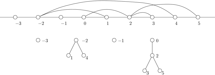
Figure 1: An example of the subtractive attachment process (up to time $5$) and the resulting forest. Here $Z_{1}=3$, $Z_{2}=2$, $Z_{3}=1$, $Z_{4}=6$, and $Z_{5}=3$.

The paper is organized as follows. In Section 2 we study whether the trees $T^{(i)}$ of the forest are finite or infinite. We show that it is the finiteness of the expectation of $Z$ that characterizes the behavior of the forest in this respect. In particular, if $\mathbb{E}Z=\infty$, then, almost surely, all trees of the forest are finite. On the other hand, if $\mathbb{E}Z<\infty$, then the forest has a unique infinite tree and the total number of non-root vertices in finite trees is finite almost surely.

In Section 3 the expected size of the trees $T_{n}^{(i)}$ is studied at time $n$. It is shown that when $Z$ has full support, the expected size of each tree at time $n$ of the forest tends to infinity, regardless of the distribution. The expected tree sizes are sublinear in $n$ if and only if $\mathbb{E}Z=\infty$.

We also study various parameters of the random trees of the forest. In Sections 5, 6, and 7 we derive results on the number of leaves, vertex degrees, and the height of the forest, respectively.

1.1 Related work

The random subtractive process studied here was examined independently, in quite different contexts, by Hammond and Sheffield [9] and Baccelli and Sodre [3], Baccelli, Haji-Mirsadeghi, and Khezeli [2], and Baccelli, Haji-Mirsadeghi, and Khaniha [1]. These papers consider an extension of the ancestral lineage process to the set $\mathbb{Z}$ of integers defined as follows: let $\{Z_{n}\}_{n\in\mathbb{Z}}$ be i.i.d. random variables taking positive integer values. This naturally defines a random graph ${\mathcal{G}}$ with vertex set $\mathbb{Z}$ such that vertices $m,n\in\mathbb{Z}$ with $m<n$ are connected by an edge if and only if $n-Z_{n}=m$. If we define the graph ${\mathcal{G}}^{(0)}$ as the subgraph of ${\mathcal{G}}$ obtained by removing all edges $(m,n)$ for which $\max(m,n)\leq 0$, then ${\mathcal{G}}^{(0)}$ is exactly the subtractive random forest studied in this paper.

It is shown in [9] — and also in [1] — that if $\sum_{n=1}^{\infty}r_{n}^{2}<\infty$, then almost surely ${\mathcal{G}}$ has a unique connected component, whereas if $\sum_{n=1}^{\infty}r_{n}^{2}=\infty$, then almost surely ${\mathcal{G}}$ has infinitely many connected components. Hammond and Sheffield are only interested in the latter (extremely heavy-tailed) case. They use the resulting coloring of the integers to define a random walk that converges to fractional Brownian motion. See also Igelbrink and Wakolbinger [10] for further results on the urn model of Hammond and Sheffield.

The paper of Baccelli and Sodre [3] considers the case when $\mathbb{E}Z<\infty$. They show that in this case the graph ${\mathcal{G}}$ has a unique doubly infinite path. This implies that the subtractive random forest ${\mathcal{G}}^{(0)}$ contains a unique infinite tree. This fact is also implied by Theorem 1 below. The fact that all trees of the forest ${\mathcal{G}}^{(0)}$ become extinct when $\mathbb{E}Z=\infty$ (part (ii) of our Theorem 3) is implicit in Proposition 4.8 of [1]. In that paper, the graph ${\mathcal{G}}$ is referred to as a Renewal Eternal Family Forest (or Renewal Eternal Family Tree when it has a single connected component).

The long-range seed bank model of Blath, Jochen, González, Kurt, and Spano [4] is also based on a similar subtractive process.

Another closely related model is studied by Chierichetti, Kumar, and Tomkins [6]. In their model, the nonnegative integers are colored by a finite number of colors and the subtractive process is not stationary. Given a sequence of positive “weights” $\{w_{i}\}_{i=1}^{\infty}$, the colors are assigned to the positive integers sequentially such that the color of $n$ is the same as the color of $n-Z_{n}$ where the distribution of $Z_{n}$ is given by $\mathbb{P}\{Z_{n}=i\}=w_{i}/\sum_{j=1}^{i}w_{j}$. (The process is initialized by assigning fixed colors to the first few positive integers.) Chierichetti, Kumar, and Tomkins are mostly interested in the existence of the limiting empirical distribution of the colors.

2 Survival and extinction

This section is dedicated to the question whether the trees $T^{(i)}$ of the subtractive random forest are finite or infinite. The main results show a sharp contrast in the behavior of the limiting random forest depending on the tail behavior of the random variable $Z$. When $Z$ has a light tail such that $\mathbb{E}Z<\infty$, then a single tree survives and the total number of non-root vertices of all the remaining trees is finite, almost surely. This is in sharp contrast to what happens when $Z$ is heavy-tailed: When $\mathbb{E}Z=\infty$, then all trees become extinct, that is, every tree in the forest is finite.

2.1 $\mathbb{E}Z<\infty$: a single infinite tree

First we consider the case when $\mathbb{E}Z<\infty$. We show that, almost surely, the forest contains a single infinite tree. Moreover, the total number of non-root vertices in all other trees is an almost surely finite random variable. In other words, the sequence of “colors” $C_{n}$ becomes constant after a random index.

Theorem 1.

Let $\mathbb{E}Z<\infty$ and assume that $q_{1}>0$. Then there exists a positive random variable $N$ with $\mathbb{P}\{N<\infty\}=1$ and a (random) index $I\in\{0,-1,\ldots\}$ such that $C_{n}=I$ for all $n\geq N$, with probability one.

Proof.   Define a Markov chain $\{B_{n}\}_{n\in\mathbb{N}}$ with state space $\mathbb{N}$ by the recursion $B_{1}=1$ and, for $n\geq 1$,

$$B_{n+1}=\left\{\begin{array}[]{ll}B_{n}+1&\text{if $Z_{n+1}\leq B_{n}$}\\ 1&\text{otherwise.}\end{array}\right.$$

Thus, $B_{n}$ defines the length of a block of consecutive vertices such that each vertex in the block (apart from the first one) is linked to a previous vertex in the same block. In particular, all vertices in the block belong to the same tree.

Note first that for any $n>1$,

$$\mathbb{P}\{B_{n}=n\} = q_{1}(q_{1}+q_{2})\cdots(q_{1}+\cdots+q_{n-1})$$

$$= \prod_{i=1}^{n-1}(1-p_{i+1})$$

$$\geq \exp\left(-\sum_{i=1}^{n-1}\frac{p_{i+1}}{1-p_{i+1}}\right)$$

$$\geq \exp\left(-\frac{1}{1-p_{2}}\sum_{i=1}^{n-1}p_{i+1}\right)$$

$$\geq \exp\left(-\frac{\mathbb{E}Z}{q_{1}}\right)~{}.$$

Since the events $\{B_{n}=n\}$ are nested, by continuity of measure we have that

$$\mathbb{P}\{B_{n}=n\ \text{for all $n\in\mathbb{N}$}\}\geq\exp\left(-\frac{\mathbb{E}Z}{q_{1}}\right)>0~{}.$$ (2.1)

Hence, with positive probability, $C_{n}=0$ for all $n\geq 1$. (Note that $\mathbb{P}\{C_{1}=0\}=q_{1}$ is positive by assumption.) Since $\{B_{n}\}_{n\in\mathbb{N}}$ is a Markov chain, this implies that, with probability one, the set $\{n:B_{n}=1\}$ is finite, which implies the theorem. We may take $N=\max\{n\in\mathbb{N}:B_{n}=1\}$ as the (random) index after which the sequence $C_{n}$ is a constant.  

Note that the assumption $q_{1}>0$ may be somewhat weakened. However, some condition is necessary to avoid periodicity. For example, if the distribution of $Z$ is concentrated on the set of even integers, then the assertion of Theorem 1 cannot hold.

The next result shows that the random index $N$ has a finite expectation if and only if $Z$ has a finite second moment.

Theorem 2.

Let $\mathbb{E}Z<\infty$ and assume that $q_{1}>0$. Consider random index $N$ defined in the proof of Theorem 1. Then $\mathbb{E}N<\infty$ if and only if $\mathbb{E}Z^{2}<\infty$. In particular, if $\mathbb{E}Z^{2}<\infty$, then the total number of vertices $n\in\mathbb{N}$ outside of the unique infinite tree has finite expectation.

Proof.   Consider the Markov chain $\{B_{n}\}_{n\in\mathbb{N}}$ defined in the proof of Theorem 1. For $i\in\mathbb{N}$, let $N_{i}=\sum_{n=1}^{\infty}\mathbbm{1}_{B_{n}=i}$ denote the number of times the Markov chain visits state $i$. The key observation is that we may write

$$N=\sum_{n=1}^{\infty}\sum_{i=1}^{\infty}i\mathbbm{1}_{B_{n}=i,B_{n+1}=1}~{}.$$

Since $\mathbb{P}\{B_{n+1}=1|B_{n}=i\}=p_{i+1}$, this implies

$$\mathbb{E}N=\sum_{i=1}^{\infty}ip_{i+1}\mathbb{E}N_{i}~{}.$$

Next, notice that $\mathbb{E}N_{2}=q_{1}\mathbb{E}N_{1}$, $\mathbb{E}N_{3}=(q_{1}+q_{2})\mathbb{E}N_{2}$, and similarly, $\mathbb{E}N_{i}=(1-p_{i})\mathbb{E}N_{i-1}=\prod_{j=2}^{i}(1-p_{j})\mathbb{E}N_{1}$. By convention, we write $\prod_{j=2}^{1}(1-p_{j})=1$. It follows from (2.1) that $N_{1}$ is stochastically dominated by a geometric random variable and therefore $\mathbb{E}N_{1}<\infty$. Thus,

$$\mathbb{E}N=\mathbb{E}N_{1}\sum_{i=1}^{\infty}ip_{i+1}\prod_{j=2}^{i}(1-p_{j})~{}.$$

As noted in the proof of Theorem 1, for all $i\geq 1$,

$$c_{0}\leq\prod_{j=2}^{i}(1-p_{j})\leq 1~{},$$

where $c_{0}\stackrel{{\scriptstyle\mathrm{def.}}}{{=}}\exp\left(-\frac{\mathbb{E}Z}{q_{1}}\right)$ is a positive constant, and therefore

$$c_{0}\mathbb{E}N_{1}\sum_{i=1}^{\infty}ip_{i+1}\leq\mathbb{E}N\leq\mathbb{E}N_{1}\sum_{i=1}^{\infty}ip_{i+1}~{}.$$

Since $\sum_{i=1}^{\infty}ip_{i+1}=(1/2)\mathbb{E}Z(Z-1)$, the theorem follows.  

2.2 $\mathbb{E}Z=\infty$: extinction of all trees

In this section we show that when $Z$ has infinite expectation, then every tree of the forest becomes extinct, almost surely. In other words, with probability one, there is no infinite tree in the random forest. This is in sharp contrast with the case when $\mathbb{E}Z<\infty$, studied in Section 2.1.

Recall that for $i\leq 0$, $S^{(i)}$ denotes the size of tree $T^{(i)}$ rooted at vertex $i$.

A set of vertices $\{n_{1},n_{2},\ldots\}\subset\{0,1,2,\ldots\}$ forms a maximal infinite path if $n_{1}<n_{2}<\cdots$, for all $k>1$, $n_{k}-Z_{n_{k}}=n_{k-1}$, and $n_{1}-Z_{n_{1}}\leq 0$.

Theorem 3.

• If $\mathbb{E}Z<\infty$, then, with probability one, there exists a unique integer $i\leq 0$ such that $S^{(i)}=\infty$ and the forest contains a unique maximal infinite path. Moreover,

  $$\mathbb{P}\left\{S^{(0)}=\infty\right\}=\frac{1}{\mathbb{E}Z}~{}.$$

• If $q_{i}>0$ for all $i\in\mathbb{N}$ and $\mathbb{E}Z=\infty$, then

  $$\mathbb{P}\left\{\exists i\leq 0:S^{(i)}=\infty\right\}=0~{}.$$

Proof.   We naturally extend the notation $T^{(i)}$ to positive integers $i\in\mathbb{N}$ so that $T^{(i)}$ is the subtree of the random forest rooted at $i$. Similarly, $S^{(i)}=|T^{(i)}|$ denotes the number of vertices in this subtree.

In Proposition 6 below we show that, regardless of the distribution of $Z$, there is no vertex of infinite degree, almost surely. This implies that the probability that the tree rooted at $0$ is infinite equals

$$\mathbb{P}\left\{S^{(0)}=\infty\right\}=\mathbb{P}\left\{\bigcup_{i\in\mathbb{N}}\left\{Z_{i}=i,S^{(i)}=\infty\right\}\right\}\leq\sum_{i\in\mathbb{N}}q_{i}\mathbb{P}\left\{S^{(i)}=\infty\right\}~{},$$ (2.2)

where we used the union bound and the fact that the events $Z_{i}=i$ and $S^{(i)}=\infty$ are independent since the latter only depends on the random variables $Z_{i+1},Z_{i+2},\ldots$. Since $\mathbb{P}\left\{S^{(i)}=\infty\right\}=\mathbb{P}\left\{S^{(0)}=\infty\right\}$ for all $i\geq 1$, the right-hand side of (2.2) equals $\mathbb{P}\left\{S^{(0)}=\infty\right\}$, that is, the inequality in (2.2) cannot be strict. This means that the events $\left\{Z_{i}=i,S^{(i)}=\infty\right\}$ for $i\in\mathbb{N}$ are disjoint (up to a zero-measure set). In particular, almost surely, there are no two maximal infinite paths meeting at vertex $0$. By countable additivity, this also implies that

$$\mathbb{P}\left\{\text{there exist two infinite paths meeting at any $i\in\mathbb{Z}$}\right\}=0~{}.$$

In particular, with probability one, all maximal infinite paths in the forest are disjoint.

Similarly to (2.2), for all $i\leq 0$,

$$\mathbb{P}\left\{S^{(i)}=\infty\right\}=\sum_{j:j+i>0}q_{j}\mathbb{P}\left\{S^{(i+j)}=\infty\right\}=\sum_{j:j+i>0}q_{j}\mathbb{P}\left\{S^{(0)}=\infty\right\}=p_{1-i}\mathbb{P}\left\{S^{(0)}=\infty\right\}~{}.$$

Hence, the expected number of trees in the forest that contain infinitely many vertices equals

$$\mathbb{E}\left[\sum_{i\leq 0}\mathbbm{1}_{S^{(i)}=\infty}\right]=\mathbb{P}\left\{S^{(0)}=\infty\right\}\sum_{i\leq 0}p_{1-i}=\mathbb{P}\left\{S^{(0)}=\infty\right\}\mathbb{E}Z~{}.$$ (2.3)

If $\mathbb{E}Z<\infty$, then by Theorem 1, the expectation on the left-hand side equals one. This implies part (i) of Theorem 3.

It remains to prove part (ii), so assume that $\mathbb{E}Z=\infty$. Suppose first that the left-hand side of (2.3) is finite. Then we must have $\mathbb{P}\left\{S^{(0)}=\infty\right\}=0$. But then $\mathbb{P}\left\{S^{(i)}=\infty\right\}=0$ for all $i\geq 0$, which implies the statement.

Finally, assume that $\mathbb{E}\left[\sum_{i\leq 0}\mathbbm{1}_{S^{(i)}=\infty}\right]=\infty$. This implies that with positive probability, there are at least two infinite trees in the forest. However, as we show below, almost surely there is at most one infinite tree in the forest. Hence, this case is impossible, completing the proof.

It remains to prove that for any $i<j\leq 0$,

$$\mathbb{P}\left\{S^{(i)}=\infty,S^{(j)}=\infty\right\}=0~{}.$$

For $i<k$, denote by $E_{i,k}=\{k-Z_{k}=i\}$ the event that $k$ is a vertex in $T^{(i)}$ connected to $i$ by an edge (i.e., $k$ is a level $1$ node in the tree $T^{(i)}$). Then by the union bound,

$$\mathbb{P}\left\{S^{(i)}=\infty,S^{(j)}=\infty\right\}\leq\sum_{k,\ell\in\mathbb{N}:k\neq\ell}q_{k-i}q_{j-\ell}\mathbb{P}\left\{S^{(k)}=\infty,S^{(\ell)}=\infty|E_{i,k},E_{j,\ell}\right\}~{}.$$

The key observation is that for all $i<j\leq 0$ and $k,\ell\in\mathbb{N}$,

$$\mathbb{P}\left\{S^{(k)}=\infty,S^{(\ell)}=\infty|E_{i,k},E_{j,\ell}\right\}=\mathbb{P}\left\{S^{(k)}=\infty,S^{(\ell)}=\infty|E_{0,k},E_{0,\ell}\right\}~{},$$

and therefore

$$\mathbb{P}\left\{S^{(i)}=\infty,S^{(j)}=\infty\right\} \leq \sum_{k,\ell\in\mathbb{N}:k\neq\ell}\frac{q_{k-i}q_{j-\ell}}{q_{k}q_{\ell}}q_{k}q_{\ell}\mathbb{P}\left\{S^{(k)}=\infty,S^{(\ell)}=\infty|E_{0,k},E_{0,\ell}\right\}$$

$$= \sum_{k,\ell\in\mathbb{N}:k\neq\ell}\frac{q_{k-i}q_{j-\ell}}{q_{k}q_{\ell}}\mathbb{P}\left\{Z_{k}=k,S^{(k)}=\infty,Z_{\ell}=\ell,S^{(\ell)}=\infty\right\}~{}.$$

However, as shown above, each term of the sum on the right-hand side equals zero, which concludes the proof.  

3 Expected tree sizes

In this section we study the expected size of the trees of the random forest. In particular, we show that in all cases (if $Z$ has full support), the expected size of each tree at time $n$ of the forest converges to infinity as $n\to\infty$. The rate of growth is sublinear if and only if $\mathbb{E}Z=\infty$.

Denote the expected size of the tree rooted at $i$ by $R_{n}^{(i)}=\mathbb{E}S_{n}^{(i)}$.

Proposition 1.

(expected tree sizes.)

• For every $i\in\{0,-1,\ldots\}$, the expected size of the tree rooted at $i$ satisfies

  $$\lim_{n\to\infty}R_{n}^{(i)}=\infty~{}.$$

  Hence, for all distributions of $Z$, we have $\mathbb{E}S^{(i)}=\infty$.

• The sequence $(R_{n}^{(0)})_{n\geq 0}$ is subadditive, that is, for all $n,m\geq 0$, $R_{n+m}^{(0)}\leq R_{n}^{(0)}+R_{m}^{(0)}$ (where we define $R_{n}^{(0)}=0$).

• For every $i\leq 0$,

  $$\lim_{n\to\infty}\frac{R_{n}^{(i)}}{n}=0\quad\text{if and only if}\quad\mathbb{E}Z=\infty~{}.$$

• If $\mathbb{E}Z<\infty$, then

  $$\lim_{n\to\infty}\frac{R_{n}^{(0)}}{n}=\frac{1}{\mathbb{E}Z}~{}.$$ (3.1)

• Also, for all distributions of $Z$ and for all $i\leq 0$ and $n\in\mathbb{N}$,

  $$R_{n}^{(i)}\leq 1+p_{1-i}R_{n}^{(0)}~{}.$$ (3.2)

Proof.   For $k\in\mathbb{N}$, let $N_{k}$ denote the number of vertices at path distance $k$ in the tree $T^{(0)}$ rooted at $0$. Then

$$\mathbb{E}N_{k} = \sum_{n=1}^{\infty}\mathbb{P}\left\{\text{vertex}\ n\ \text{connects to $0$ in $k$ steps}\right\}$$

$$= \sum_{n=k}^{\infty}\mathbb{P}\left\{X_{1}+\cdots+X_{k}=n\right\}$$

(where $$X_{1},\ldots,X_{k} Z$$ are i.i.d. with the same distribution as )

$$= \mathbb{P}\left\{X_{1}+\cdots+X_{k}\geq k\right\}=1~{}.$$

Hence, $\mathbb{E}S^{(0)}=\sum_{k\in\mathbb{N}}\mathbb{E}N_{k}=\infty$, proving $(1)$ for the tree rooted at $0$.

In order to relate expected tree sizes rooted at different vertices $i$, we may consider subtrees rooted at vertices $j\in\{1,2,\ldots\}$. To this end, let $T^{(j)}_{n}$ denote the subtree of the forest rooted at $j$ at time $n$ and let $S^{(j)}_{n}$ be its size. Then the size of the tree rooted at $i\in\{0,-1,\ldots\}$ satisfies

$$S^{(i)}_{n}=1+\sum_{j=1}^{n}\mathbbm{1}_{j-Z_{j}=i}S^{(j)}_{n}~{}.$$

Noting that $S^{(j)}_{n}$ is independent of $Z_{j}$ and that $S^{(j)}_{n}$ has the same distribution as $S^{(0)}_{n-j}$, we obtain the identity

$$R_{n}^{(i)}=1+\sum_{j=1}^{n}q_{j-i}R_{n-j}^{(0)}~{}.$$

Let $\ell$ be the least positive integer such that $q_{\ell-i}$ is strictly positive. The identity above implies that $R_{n}^{(i)}\geq q_{\ell-i}R_{n-\ell}^{(0)}$, and therefore $\lim_{n\to\infty}R_{n}^{(i)}=\infty$ for all $i$, proving the first assertion of the theorem.

Using the fact that $R_{n-j}^{(0)}\leq R_{n}^{(0)}$ for all $j\in[n]$, we obtain (3.2).

Taking $i=0$ in the equality above, we obtain the following recursion for the expected size of the tree rooted at $0$, at time $n\in\mathbb{N}$:

$$R_{n}^{(0)}=1+\sum_{t=1}^{n}q_{t}R_{n-t}^{(0)}~{}.$$ (3.3)

We may use the reursive formula to prove subadditivity of the sequence $(R_{n}^{(0)})_{n\geq 0}$. We proceed by induction. $R_{n+m}^{(0)}\leq R_{n}^{(0)}+R_{m}^{(0)}$ holds trivially for all $m\geq 0$ when $n=0$. Let $k\geq 1$. Suppose now that the inequality holds for all $n\leq k$ and $m\geq 0$. Then by (3.3),

$$R_{k+m+1}^{(0)} = R_{k+1}^{(0)}+\sum_{t=1}^{k+1}q_{t}\left(R_{k+m+1-t}^{(0)}-R_{k+1-t}^{(0)}\right)+\sum_{t=k+2}^{k+m+1}q_{t}R_{k+m+1-t}^{(0)}$$

$$\leq R_{k+1}^{(0)}+\sum_{t=1}^{k+1}q_{t}R_{m}^{(0)}+\sum_{t=k+2}^{k+m+1}q_{t}R_{k+m+1-t}^{(0)}$$

(by the induction hypothesis)

$$\leq R_{k+1}^{(0)}+\sum_{t=1}^{k+1}q_{t}R_{m}^{(0)}+\sum_{t=k+2}^{k+m+1}q_{t}R_{m}^{(0)}$$

(since $$R_{n}^{(0)}$$ is nondecreasing)

$$\leq R_{k+1}^{(0)}+R_{m}^{(0)}~{},$$

proving $(2)$.

Next we show that if $\mathbb{E}Z=\infty$ then $R_{n}^{(0)}/n\to 0$. To this end, observe that by (3.3), we have

$$\sum_{i=1}^{n}R_{n}^{(0)} = n+\sum_{i=1}^{n}\sum_{t=1}^{i}q_{t}R_{i-t}^{(0)}=n+\sum_{i=1}^{n}\sum_{t=0}^{i-1}q_{i-t}R_{t}^{(0)}$$

$$= n+\sum_{t=0}^{n-1}R_{t}^{(0)}\sum_{i=t+1}^{n}q_{i-t}=n+\sum_{t=0}^{n-1}R_{t}^{(0)}(1-p_{n-t+1})~{}.$$

Thus,

$$n=R_{n}^{(0)}+\sum_{t=0}^{n-1}R_{t}^{(0)}p_{n-t+1}\geq R_{n}^{(0)}+R_{\lfloor n/2\rfloor}^{(0)}\sum_{t=\lfloor n/2\rfloor}^{n-1}p_{n-t+1}\geq R_{\lfloor n/2\rfloor}^{(0)}\sum_{t=2}^{\lfloor n/2\rfloor}p_{t}~{}.$$

Hence,

$$\frac{R_{\lfloor n/2\rfloor}^{(0)}}{n}\leq\frac{1}{\sum_{t=2}^{\lfloor n/2\rfloor}p_{t}}\to 0~{}.$$

It remains to prove (3.1). (Note that (3.1) implies that $R_{n}^{(i)}/n$ is bounded away from zero for all $i\leq 0$ and therefore if $R_{n}^{(i)}/n\to 0$ for some $i\leq 0$ then $\mathbb{E}Z=\infty$.) To this end, let

$$f(z)=\sum_{n=0}^{\infty}R_{n}^{(0)}z^{n}$$

be the generating function of the sequence $\{R_{n}^{(0)}\}_{n\geq 0}$, where $z$ is a complex variable. Using the recursion (3.3), we see that

$$f(z) = \sum_{n=0}^{\infty}z^{n}+\sum_{n=1}^{\infty}\sum_{t=1}^{n}q_{t}R_{n-t}^{(0)}z^{n}$$

$$= \sum_{n=0}^{\infty}z^{n}+\sum_{t=1}^{\infty}q_{t}z^{t}\sum_{n=t}^{\infty}R_{n-t}^{(0)}z^{n-t}$$

$$= \frac{1}{1-z}+Q(z)f(z)~{},$$

where $Q(z)=\sum_{n=1}^{\infty}q_{n}z^{n}$ is the generating function of the sequence $\{q_{n}\}_{n\geq 1}$. Thus, we have

$$f(z)=\frac{1}{(1-z)(1-Q(z))}~{}.$$

Recall that we assume here that $\mathbb{E}Z<\infty$. Since $1-Q(z)\sim(1-z)\sum_{n=1}^{\infty}nq_{n}=(1-z)\mathbb{E}Z$ when $z\to 1$, we have

$$f(z)\sim\frac{1}{(1-z)^{2}\mathbb{E}Z}\quad\text{when $z\to 1$}~{}.$$

(3.1) now follows from Corollary VI.1 of Flajolet and Sedgewick [8].  

Remark 1.

(profile of the $0$-tree.) Note that we proved in passing that, regardless of the distribution, for all $k\in\mathbb{N}$, the number $N_{k}$ of vertices in the tree $T^{(0)}$ that are at path distance $k$ from the root satisfies $\mathbb{E}N_{k}=1$. The sequence $\{N_{k}\}_{k=1}^{\infty}$ is often called the profile of the tree $T^{(0)}$.

Remark 2.

(expected vs. actual size.) While Proposition 1 summarizes the properties of the expected tree sizes $R_{n}^{(i)}=\mathbb{E}S_{n}^{(i)}$, it is worth emphasizing that the random variables $S_{n}^{(i)}$ behave very differently. For example, when $\mathbb{E}Z=\infty$, then we know from Theorem 3 that for each $i\leq 0$, $S^{(i)}=\limsup_{n\to\infty}S_{n}^{(i)}<\infty$, while, by Proposition 1, $\mathbb{E}S_{n}^{(i)}\to\infty$. Also note that, for all distributions of $Z$, for each $i\leq 0$, $\mathbb{P}\{S^{(i)}=1\}$ is strictly positive and therefore $S_{n}^{(i)}$ does not concentrate.

4 The number of trees of the forest

In this section we study the number $M_{n}=\sum_{i\in\{0,-1,-2,\ldots\}}\mathbbm{1}_{S^{(i)}_{n}>1}$ of trees in the random forest that have at least one vertex $t\in[n]$ attached to the root $i$. In the motivating topic recommendation problem, this random variable describes the number of topics that are recommended by time $n$.

We show that the expected number of trees $\mathbb{E}M_{n}$ goes to infinity as $n\to\infty$ if and only if $\mathbb{E}Z=\infty$. Moreover, $M_{n}\sim m_{n}$ in probability, where $m_{n}=\mathbb{E}\left[\min(Z,n)\right]$.

Note that it follows from Theorem 3 that if $\mathbb{E}Z=\infty$, then $M_{n}\to\infty$ almost surely.

In order to understand the behavior of $M_{n}$, we first study the random variable

$$O_{n}=\sum_{t=1}^{n}\mathbbm{1}_{Z_{t}\geq t}~{}.$$

Note that when $Z_{t}\geq t$, then vertex $t$ connects directly to the root $t-Z_{t}\leq 0$. Hence, $O_{n}$ is the number of vertices in the forest at depth $1$ (i.e., at graph distance $1$ from the root of the tree containing the vertex). Equivalently, $O_{n}=\sum_{i\in\{0,-1,\ldots\}}D_{n}^{(i)}$ is the sum of the degrees of the roots of all trees in the forest at time $n$.

Proposition 2.

(number of trees.) The random variables $M_{n}$ and $O_{n}$ satisfy the following:

• $\mathbb{E}O_{n}=m_{n}$ ;

• If $\mathbb{E}Z=\infty$, then $(O_{n}-m_{n})/\sqrt{m_{n}}$ ; converges, in distribution, to a standard normal random variable.

• $M_{n}\leq O_{n}$ and if $\mathbb{E}Z=\infty$, then $\mathbb{E}[O_{n}-M_{n}]=o(m_{n})$.

• If $\mathbb{E}Z=\infty$, then $M_{n}/m_{n}\to 1$ in probability.

• For all $x>0$,

  $$\mathbb{P}\{M_{n}>\mathbb{E}M_{n}+x\}\leq\left(\frac{\mathbb{E}M_{n}}{\mathbb{E}M_{n}+x}\right)^{\mathbb{E}M_{n}+x}e^{-x}$$

  and

  $$\mathbb{P}\{M_{n}<\mathbb{E}M_{n}-x\}\leq e^{-x^{2}/(2\mathbb{E}M_{n})}~{}.$$

Proof.   Note that $O_{n}$ is a sum of independent Bernoulli random variables and

$$\mathbb{E}O_{n}=\sum_{t=1}^{n}p_{t}=m_{n}~{}.$$

To prove (ii), we may use Lyapunov’s central limit theorem. Indeed,

$$\mathrm{Var}(O_{n})=\sum_{t=1}^{n}p_{t}(1-p_{t})=m_{n}-\sum_{t=1}^{n}p_{t}^{2}~{}.$$

If $\mathbb{E}Z=\infty$, then $\sum_{t=1}^{n}p_{t}^{2}=o(m_{n})$. (This simply follows from the fact that $p_{t}\to 0$.) In order to use Lyapunov’s central limit theorem, it suffices that

$$\frac{\sum_{t=1}^{n}\mathbb{E}|\mathbbm{1}_{Z_{t}\geq t}-p_{t}|^{3}}{\mathrm{Var}(O_{n})^{3/2}}\to 0~{}.$$

This follows from

$$\sum_{t=1}^{n}\mathbb{E}|\mathbbm{1}_{Z_{t}\geq t}-p_{t}|^{3}=\sum_{t=1}^{n}p_{t}(1-p_{t})\left((1-p_{t})^{2}+p_{t}^{2}\right)\leq\mathrm{Var}(O_{n})~{}.$$

In order to prove (iii), observe that for each $i\in\{0,-1,-2,\ldots\}$,

$$\mathbb{E}\mathbbm{1}_{S^{(i)}_{n}>1}=1-\mathbb{P}\left\{S^{(i)}_{n}=1\right\}=1-\prod_{t=1}^{n}(1-q_{t-i})~{},$$

and therefore

$$\mathbb{E}M_{n} \geq \sum_{i\leq 0}\left(1-e^{-\sum_{t=1}^{n}q_{t-i}}\right)$$

$$= \sum_{i\leq 0}\left(1-e^{-(p_{1-i}-p_{n+1-i})}\right)$$

$$\geq \sum_{i\leq 0}(p_{1-i}-p_{n+1-i})-\frac{1}{2}\sum_{i\leq 0}(p_{1-i}-p_{n+1-i})^{2}$$

(using $$e^{-x}\leq 1-x+x^{2}/2 x\geq 0$$ for )

$$= \sum_{t=1}^{n}p_{t}-\frac{1}{2}\sum_{i\leq 0}(p_{1-i}-p_{n+1-i})^{2}=m_{n}(1-o(1))~{},$$

where the last assertion follows from the fact that $p_{1-i}-p_{n+1-i}\to 0$ as $i\to-\infty$ and that $\sum_{t=1}^{n}p_{t}\to\infty$ when $\mathbb{E}Z=\infty$. Part (iv) simply follows from (ii), (iii), and Markov’s inequality. Indeed, $M_{n}\leq O_{n}$ and for every $\epsilon>0$,

$$\mathbb{P}\left\{O_{n}-M_{n}>\epsilon m_{n}\right\}\leq\frac{\mathbb{E}[O_{n}-M_{n}]}{\epsilon m_{n}}=o(1)~{}.$$

The exponential inequalities of (v) follow from the fact that the collection of indicator random variables $\left\{\mathbbm{1}_{Z_{n}=n-i}\right\}_{n\geq 1,i\leq 0}$ is negatively associated (Dubhashi and Ranjan [7, Proposition 11]). This implies that the collection of indicators

$$\left\{\mathbbm{1}_{S^{(i)}_{n}>1}\right\}_{i\leq 0}=\left\{\mathbbm{1}_{\sum_{t=1}^{n}\mathbbm{1}_{Z_{t}=t-i}>0}\right\}_{i\leq 0}$$

is also negatively associated ([7, Proposition 7]). Hence, by [7, Proposition 5], the tail probabilities of the sum $M_{n}=\sum_{i\leq 0}\mathbbm{1}_{S^{(i)}_{n}>1}$ satisfy the Chernoff bounds for the corresponding sum of independent random variables. The inequalities of (v) are two well-known examples of the Chernoff bound (see, e.g., [5]).  

5 Number of leaves

Let $L_{n}$ denote the number of leaves of the tree rooted at $0$, at time $n$. That is, $L_{n}$ is the number of vertices $t\in[n]$ such that $C_{t}=0$ and no vertex $s\in\{t+1,\ldots,n\}$ is attached to it. Recall that $r_{n}=\mathbb{P}\{C_{n}=0\}$ is the probability that vertex $n$ belongs to the tree $T_{n}^{(0)}$ rooted at $0$ and $R_{n}^{(0)}=\sum_{t=1}^{n}r_{t}$ is the expected size of the tree $T_{n}^{(0)}$. The following proposition shows that the expected number of leaves is proportional to the expected number of vertices in the tree.

Proposition 3.

(number of leaves.) Denote $q_{max}=\max_{n}q_{n}$. If $\mathbb{E}Z=\infty$, then there exists a constant $c\in[e^{-1/(1-q_{max})},e^{-1}]$ such that

$$\lim_{n\to\infty}\frac{\mathbb{E}L_{n}}{R_{n}^{(0)}}=c~{}.$$

Proof.   Let $t\in[n]$. Since the event $\{C_{t}=0\}$ is independent of the event that no vertex $s\in\{t+1,\ldots,n\}$ is attached to $t$, we may write

$$\mathbb{E}L_{n} = \sum_{t=1}^{n}r_{t}\prod_{s=t+1}^{n}(1-q_{s-t})$$

$$= \sum_{t=1}^{n}r_{t}\prod_{s=1}^{n-t}(1-q_{s})$$

$$= \sum_{t=1}^{n}r_{t}e^{\sum_{s=1}^{n-t}\log(1-q_{s})}~{}.$$

The sequence $\left(\sum_{s=1}^{n}\log(1-q_{s})\right)_{n\geq 1}$ is monotone decreasing and, using that $\log(1-x)\geq-x/(1-x)$ for $x\geq 0$,

$$\sum_{s=1}^{n}\log(1-q_{s})\geq\sum_{s=1}^{n}\frac{-q_{s}}{1-q_{s}}\geq\sum_{s=1}^{n}\frac{-q_{s}}{1-q_{s}}\geq\frac{-1}{1-q_{max}}~{}.$$

Thus, there exists $c\geq e^{-1/(1-q_{max})}$ such that for all $\epsilon>0$, there exists $n_{0}\in\mathbb{N}$ such that $|e^{\sum_{s=1}^{n}\log(1-q_{s})}-c|<\epsilon$ whenever $n>n_{0}$. But then

$$\left|\mathbb{E}L_{n}-cR_{n}^{(0)}\right| = \left|\sum_{t=1}^{n}r_{t}\left(e^{\sum_{s=1}^{n-t}\log(1-q_{s})}-c\right)\right|$$

$$\leq n_{0}+\epsilon\sum_{t=1}^{n-n_{0}}r_{t}$$

$$\leq \epsilon R_{n}^{(0)}+O(1)~{}.$$

To see why $c\leq 1/e$, note that

$$\sum_{s=1}^{n}\log(1-q_{s})\leq-\sum_{s=1}^{n}q_{s}\to-1~{}.$$

 

Remark 3.

(expected vs. actual random number of leaves.) Just like the size of the trees, the number of leaves $L_{n}$ is not concentrated around its expectation. Indeed, when $\mathbb{E}Z=\infty$, $L_{n}\leq S^{(0)}$ is an almost surely bounded sequence of random variables, whereas $\mathbb{E}L_{n}\to\infty$ by Propositions 1 and 3.

Remark 4.

(number of leaves when $\mathbb{E}Z<\infty$) Proposition 1 is only concerned with the case $\mathbb{E}Z=\infty$. When $Z$ has finite expectation, then the number of leaves of the tree rooted at $0$ depends on whether the tree survives or not. Recall that the events $S^{(0)}<\infty$ and $S^{(0)}=\infty$ both have positive probability. It is easy to see that, conditioned on the event $S^{(0)}=\infty$, the ratio $L_{n}/S_{n}^{(0)}$ almost surely converges to $\mathbb{P}\{S^{(0)}=1\}$. On the other hand, conditioned on the event $S^{(0)}<\infty$, $L_{n}/S_{n}^{(0)}$ converges to a nontrivial random variable taking values in $[0,1]$.

6 Degrees

The outdegree $D_{n}^{(i)}$ of a vertex $i\in\mathbb{Z}$ is the number of vertices attached to it at time $n\in\mathbb{N}$, that is,

$$D_{n}^{(i)}=\sum_{t=\max(1,i+1)}^{n}\mathbbm{1}_{Z_{t}=t-i}~{}.$$

We also write

$$D^{(i)}=\sum_{t=\max(1,i+1)}^{\infty}\mathbbm{1}_{Z_{t}=t-i}$$

for the degree of vertex $i$ in the random forest at the end of the attachment process. Note that for all root vertices $i\leq 0$, $\mathbb{E}D_{n}^{(i)}=\sum_{t=1}^{n}q_{t-i}=p_{1-i}-p_{n-i+1}$ and $\mathbb{E}D^{(i)}=p_{1-i}$, while for all other vertices $i\geq 1$, $\mathbb{E}D_{n}^{(i)}=1-p_{n-i+1}$ and $\mathbb{E}D^{(i)}=1$.

First we show that the degrees among all root vertices is a tight sequence of random variables under general conditions, with the possible exception of some extremely heavy-tailed distributions.

Proposition 4.

(maximum root degree.) If the distribution of $Z$ is such that there exists $\lambda>0$ such that $\sum_{n=1}^{\infty}p_{n}^{\lambda}<\infty$, then the root degrees $\{D^{(i)}\}_{i<0}$ form a tight sequence of random variables. In particular, for all $x\geq\lambda$, we have

$$\mathbb{P}\left\{\max_{i<0}D^{(i)}>x\right\}\leq\left(\frac{e}{x}\right)^{x}\sum_{n=1}^{\infty}p_{n}^{x}~{}.$$

As an example, consider a distribution with polynomially decaying tail such that $q_{n}=\Theta(n^{-1-\alpha})$ for some $\alpha>0$. Then $p_{n}=\Theta(n^{-\alpha})$, and then for any $x>1/\alpha$, we have $\sum_{n=1}^{\infty}p_{n}^{x}<\infty$. However, if $q_{n}$ decreases much slower, for example, if $q_{n}\sim 1/(n\log^{2}n)$, then the proposition does not guarantee tightness of the root degrees.

Proof.  We have

$$\mathbb{P}\left\{\max_{i<0}D^{(i)}>x\right\} \leq \sum_{i\leq 0}\mathbb{P}\left\{\sum_{t=1}^{\infty}\mathbbm{1}_{Z_{t}=t-i}>x\right\}$$

$$\leq \sum_{i\leq 0}\exp\left(x-p_{1-i}-x\log\frac{x}{p_{1-i}}\right)$$

(by the Chernoff bound)

$$\leq \sum_{i\leq 0}\exp\left(x-x\log\frac{x}{p_{1-i}}\right)$$

$$= \left(\frac{e}{x}\right)^{x}\sum_{n=1}^{\infty}p_{n}^{x}~{},$$

which proves the claim.  

Next we show that the maximum degree of any vertex $t\in[n]$ grows at most as the maximum of independent Poisson$(1)$ random variables that is well known (and easily seen) to grow as $\log n/\log\log n$.

Proposition 5.

(maximum degree.) For every $\epsilon>0$, with probability tending to $1$,

$$\max_{t\in[n]}D^{(t)}\leq(1+\epsilon)\frac{\log n}{\log\log n}~{}.$$

Proof.   The proof once again follows from a simple application of the Chernoff bound for sums of independent Bernoulli random variables: for any $x>0$,

$$\mathbb{P}\left\{\max_{t\in[n]}D^{(t)}>x\right\}\leq ne^{x-1-x\log x}~{},$$ (6.1)

which converges to $0$ if $x=(1+\epsilon)\frac{\log n}{\log\log n}$ for any fixed $\epsilon>0$.  

Proposition 6.

(all degrees are finite.) With probability $1$, $D^{(t)}<\infty$ for all $t\in\mathbb{Z}$.

Proof.   Bounding as in the proof of Proposition 4, we see that, for every $n\in\mathbb{N}$ and $x>0$,

$$\mathbb{P}\left\{\max_{i\in\{0,-1,\ldots,-n\}}D^{(i)}>x\right\}\leq n\exp\left(-x\log\frac{x}{e}\right)~{}.$$

Hence, by the Borel-Cantelli lemma, $\max_{i\in\{0,-1,\ldots,-n\}}D^{(t)}\leq 3\log n$ for all but finitely many values of $n$, almost surely. This implies that, almost surely, $D^{(t)}<\infty$ for all $t\leq 0$.

Similarly, by taking (say) $x=3\log n$ in (6.1), it follows from the Borel-Cantelli lemma that, almost surely, $\max_{t\in[n]}D^{(t)}\leq 3\log n$ for all but finitely many values of $n$. This implies that $D^{(t)}<\infty$ for all $t\in\mathbb{N}$, with probability one.  

Remark 5.

(asymptotic distribution of the out-degree.) As argued above, the asymptotic degree of vertex $i$ may be represented as a sum of independent Bernoulli random variables

$$D^{(i)}=\sum_{t=\max(1,i+1)}^{\infty}\mathbbm{1}_{Z_{t}=t-i}=\sum_{t=\max(1,i+1)}^{\infty}\text{Ber}(q_{t-i})~{}.$$

For example, for all $i\geq 0$, the $D^{(i)}$ are discrete random variables with the same distribution, satisfying $\mathbb{E}D^{(i)}=1$ and $\mathrm{Var}(D^{(i)})=1-\sum_{t=1}^{\infty}q_{t}^{2}$.

7 The height of the random forest

In this section we study the expected height of the random forest. The height $H_{n}$ of the forest, at time $n\in\mathbb{N}$, is the length of the longest path of any vertex $t\in[n]$ to the root of its tree. In Proposition 7 we derive an upper bound for $\mathbb{E}H_{n}$. The upper bound implies that the expected height is sublinear whenever $q_{n}=\Theta(n^{-1-\alpha})$ for some $\alpha\in(0,1)$.

In Proposition 8 we show that the expected height $H^{(0)}_{n}$ of the tree rooted at vertex $0$ goes to infinity, regardless of the distribution of $Z$. Of course, this implies that $\mathbb{E}H_{n}\to\infty$. As a corollary, we also show that for all distributions, $H_{n}\to\infty$ almost surely. This is to be contrasted with the fact that when $\mathbb{E}Z=\infty$, $H^{(0)}_{n}$ is almost surely bounded (just like the height of any tree in the forest).

Proposition 7.

(upper bound for the expected height of the forest.) For all distributions of $Z$, we have

$$\mathbb{E}H_{n}\leq\frac{2+\log n}{p_{n}}~{}.$$

Proof.   The path length of a vertex $n$ to the root of its tree exceeds $k$ if and only if

$$\underbrace{Z_{n}+Z_{n-Z_{n}}+Z_{n-Z_{n}-Z_{n-Z_{n}}}+\cdots}_{\text{$k$ times}}<n$$

Thus, if $X_{1},\ldots,X_{k}$ are i.i.d. with the same distribution as $Z$,

$$\mathbb{P}\left\{H_{n}>k\right\} \leq \sum_{t=1}^{n}\mathbb{P}\left\{X_{1}+\cdots+X_{k}<t\right\}$$

$$\leq \sum_{t=1}^{n}\mathbb{P}\left\{Z<t\right\}^{k}$$

$$= \sum_{t=1}^{n}\left(1-\mathbb{P}\left\{Z\geq t\right\}\right)^{k}$$

$$\leq \sum_{t=1}^{n}e^{-kp_{t}}~{}.$$

This implies that

$$\mathbb{E}H_{n} = \sum_{k=0}^{\infty}\mathbb{P}\left\{H_{n}>k\right\}$$

$$\leq \sum_{k=0}^{\infty}\min\left(1,\sum_{t=1}^{n}e^{-kp_{t}}\right)$$

$$\leq \sum_{k=0}^{\infty}\min\left(1,ne^{-kp_{n}}\right)$$

$$\leq \frac{\log n}{p_{n}}+\sum_{k=\left\lceil\frac{\log n}{p_{n}}\right\rceil}^{\infty}ne^{-kp_{n}}$$

$$\leq \frac{\log n}{p_{n}}+\frac{1}{1-e^{-p_{n}}}~{}.$$

Using the fact that $e^{-x}\geq 1-x/2$ for $x\in[0,1]$, we obtain the announced inequality.  

Proposition 8.

(lower bound for the expected height of the forest.) For all distributions of $Z$, the expected height of the tree rooted at vertex $0$ satisfies

$$\lim_{n\to\infty}\mathbb{E}H^{(0)}_{n}=\infty~{}.$$

Proof.   Since $H^{(0)}_{n}$ is an increasing sequence of random variables, we may define $H^{(0)}=\lim_{n\to\infty}H^{(0)}_{n}$ (that may be infinite). By the monotone convergence theorem, it suffices to prove that $\mathbb{E}H^{(0)}=\infty$, or equivalently, that

$$\sum_{k=1}^{\infty}\mathbb{P}\left\{H^{(0)}\geq k\right\}=\infty~{}.$$ (7.1)

Denote by $t\to_{k}0$ the event that vertex $t>0$ is connected to vertex $0$ via a path of length $k$, that is,

$$\underbrace{Z_{t}+Z_{t-Z_{t}}+Z_{t-Z_{t}-Z_{t-Z_{t}}}+\cdots}_{\text{$k$ terms}}=t$$

and define $r_{t,k}=\mathbb{P}\left\{t\to_{k}0\right\}$.

Introducing the random variable

$$N_{k}=\sum_{t=k}^{\infty}\sum_{\ell=k}^{2k-1}\mathbbm{1}_{t\to_{\ell}0}~{},$$

note that

$$\mathbb{P}\left\{H^{(0)}\geq k\right\}\geq\mathbb{P}\left\{H^{(0)}\in[k,2k-1]\right\}=\mathbb{P}\{N_{k}\geq 1\}~{}.$$

In order to derive a lower bound for $\mathbb{P}\{N_{k}\geq 1\}$, note first that

$$\mathbb{E}N_{k}=\sum_{\ell=k}^{2k-1}\mathbb{P}\{X_{1}+\cdots+X_{\ell}\geq k\}=k$$

where $X_{1},\ldots,X_{k}$ are i.i.d. with the same distribution as $Z$. By the Paley-Zygmund inequality,

$$\mathbb{P}\{N_{k}\geq 1\}\geq\left(1-\frac{1}{k}\right)^{2}\frac{\left(\mathbb{E}N_{k}\right)^{2}}{\left(\mathbb{E}N_{k}^{2}\right)}~{}.$$

In the argument below we show that $\mathbb{E}N_{k}^{2}\leq 4k^{3}$. Substituting into the inequality above, we obtain

$$\mathbb{P}\left\{H^{(0)}\geq k\right\}\geq\mathbb{P}\{N_{k}\geq 1\}\geq\left(1-\frac{1}{k}\right)^{2}\frac{1}{4k}~{},$$

concluding the proof of $\mathbb{E}H^{(0)}=\infty$.

Hence, it remains to derive the announced upper bound for the second moment of $N_{k}$. First note that for any $t,t^{\prime}\geq k$ and $\ell,\ell^{\prime}\in\{k,k+1,\ldots,2k-1\}$

$$\mathbb{P}\{t\to_{\ell}0,t^{\prime}\to_{\ell^{\prime}}0\}\leq\sum_{m=0}^{\min(\ell,\ell^{\prime})}\sum_{s=0}^{\min(t,t^{\prime})}r_{s,m}r_{t-s,\ell-m}r_{t^{\prime}-s,\ell^{\prime}-m}~{}.$$

Then

$$\mathbb{E}N_{k}^{2} = \sum_{t=k}^{\infty}\sum_{t^{\prime}=k}^{\infty}\sum_{\ell=k}^{2k-1}\sum_{\ell^{\prime}=k}^{2k-1}\sum_{m=0}^{\min(\ell,\ell^{\prime})}\sum_{s=0}^{\min(t,t^{\prime})}r_{s,m}r_{t-s,\ell-m}r_{t^{\prime}-s,\ell^{\prime}-m}$$

$$\leq \sum_{t=k}^{\infty}\sum_{\ell=k}^{2k-1}\sum_{\ell^{\prime}=k}^{2k-1}\sum_{m=0}^{\min(\ell,\ell^{\prime})}\sum_{s=0}^{\min(t,t^{\prime})}r_{s,m}r_{t-s,\ell-m}\quad\text{(using $\sum_{t^{\prime}=k}^{\infty}r_{t^{\prime}-s,\ell^{\prime}-m}\leq 1$)}$$

$$\leq 2k\sum_{t=k}^{\infty}\sum_{\ell=k}^{2k-1}\sum_{\ell^{\prime}=k}^{2k-1}r_{t,\ell}\quad\text{(since for each $m$, $\sum_{s=1}^{\min(t,t^{\prime})}r_{s,m}r_{t-s,\ell-m}\leq r_{t,\ell}$)}$$

$$\leq 4k^{2}\sum_{t=k}^{\infty}\sum_{\ell=k}^{2k-1}r_{t,\ell}$$

$$= 4k^{2}\mathbb{E}N_{k}=4k^{3}~{},$$

as desired.  

Proposition 9.

(almost sure lower bound for the height of the forest.) For all distributions of $Z$, $\lim_{n\to\infty}H_{n}=\infty$ almost surely.

Proof.   For $\mathbb{E}Z<\infty$, the statement follows from Theorem 1 and Proposition 6 so we may assume that $Z$ has infinite expectation.

Since by Proposition 8 the expected height of the tree rooted at $0$ has infinite expectation, it follows that the distribution of $H^{(0)}$ has unbounded support.

Since by Theorem 3 the tree $T^{(0)}$ rooted at $0$ becomes extinct almost surely, the random variable $Y_{1}$ denoting the index of the last vertex that belongs to $T^{(0)}$ is almost surely finite. Let $A_{1}=H^{(0)}$ denote the height of the $0$-tree. Now we may define $Y_{2}$ such that $Y_{1}+1+Y_{2}$ is the last vertex that belongs to the tree $T^{(Y_{1}+1)}$, and let $A_{2}$ denote the height of this tree. By continuing recursively, we obtain a sequence $A_{1},A_{2},\ldots$ of i.i.d. random variables distributed as $H^{(0)}$. Moreover, $\lim_{n\to\infty}H_{n}\geq\sup_{i}A_{i}$, proving the statement.  

Acknowledgements. We are grateful to an anonymous referee for suggestions that lead to a much improved version of the paper.

References

- Baccelli et al., [2022] Baccelli, F., Haji-Mirsadeghi, M.-O., and Khaniha, S. (2022). Coupling from the past for the null recurrent Markov chain. arXiv preprint arXiv:2203.13585.
- Baccelli et al., [2018] Baccelli, F., Haji-Mirsadeghi, M.-O., and Khezeli, A. (2018). Eternal family trees and dynamics on unimodular random graphs. Unimodularity in randomly generated graphs, 719:85–127.
- Baccelli and Sodre, [2019] Baccelli, F. and Sodre, A. (2019). Renewal processes, population dynamics, and unimodular trees. Journal of Applied Probability, 56(2):339–357.
- Blath et al., [2013] Blath, J., González Casanova, A., Kurt, N., and Spano, D. (2013). The ancestral process of long-range seed bank models. Journal of Applied Probability, 50(3):741–759.
- Boucheron et al., [2013] Boucheron, S., Lugosi, G., and Massart, P. (2013). Concentration Inequalities: A Nonasymptotic Theory of Independence. Oxford University Press.
- Chierichetti et al., [2020] Chierichetti, F., Kumar, R., and Tomkins, A. (2020). Asymptotic behavior of sequence models. In Proceedings of The Web Conference 2020, pages 2824–2830.
- Dubhashi and Ranjan, [1998] Dubhashi, D. and Ranjan, D. (1998). Balls and bins: a study in negative dependence. Random Structures & Algorithms, 13(2):99–124.
- Flajolet and Sedgewick, [2009] Flajolet, P. and Sedgewick, R. (2009). Analytic Combinatorics. Cambridge University Press.
- Hammond and Sheffield, [2013] Hammond, A. and Sheffield, S. (2013). Power law Pólya’s urn and fractional Brownian motion. Probability Theory and Related Fields, 157(3):691–719.
- Igelbrink and Wakolbinger, [2022] Igelbrink, J. L. and Wakolbinger, A. (2022). Asymptotic gaussianity via coalescence probabilites in the Hammond-Sheffield urn. arXiv e-prints, pages arXiv–2201.