Real-time broadening of bath-induced density profiles
from closed-system correlation functions

Abstract

The Lindblad master equation is one of the main approaches to open quantum systems. While it has been widely applied in the context of condensed matter systems to study properties of steady states in the limit of long times, the actual route to such steady states has attracted less attention yet. Here, we investigate the nonequilibrium dynamics of spin chains with a local coupling to a single Lindblad bath and analyze the transport properties of the induced magnetization. Combining typicality and equilibration arguments with stochastic unraveling, we unveil for the case of weak driving that the dynamics in the open system can be constructed on the basis of correlation functions in the closed system, which establishes a connection between the Lindblad approach and linear response theory at finite times. In this way, we provide a particular example where closed and open approaches to quantum transport agree strictly. We demonstrate this fact numerically for the spin-1/2 XXZ chain at the isotropic point and in the easy-axis regime, where superdiffusive and diffusive scaling is observed, respectively.

I Introduction

Understanding the dynamics of many-body quantum systems has seen remarkable progress in recent years [1], including the origin of thermalization and hydrodynamics under unitary time evolution [2, 3, 4, 5], the possibility of weak and strong forms of ergodicity breaking [6, 7], and the emergence of universality far from equilibrium [8, 9, 10, 11, 12]. In addition to theoretical breakthroughs, these and related areas have also profited immensely from experiments like seminal quantum simulators, where both closed and open systems can be probed [13, 14, 15]. The competition of internal quantum dynamics, dissipation, and external driving opens up a vast landscape of exotic nonequilibrium phenomena [16, 17].

In systems with a conservation law, e.g., spin models with conserved total magnetization, a key role is played by the slow relaxation of the corresponding hydrodynamic modes [18]. While chaotic systems are typically expected to exhibit diffusion [19, 20, 21], anomalous transport can occur, e.g., in the presence of long-range interactions [22, 23, 24], in disordered and kinetically constrained systems [25, 26, 27], or in the case of integrable models [28]. For the latter, the concept of generalized hydrodynamics provides a powerful framework to predict the emerging transport behavior [29, 30]. In generic systems, in contrast, extracting quantitative values of transport coefficients like diffusion constants remains a formidable challenge even for sophisticated numerical techniques [31, 32, 33, 34].

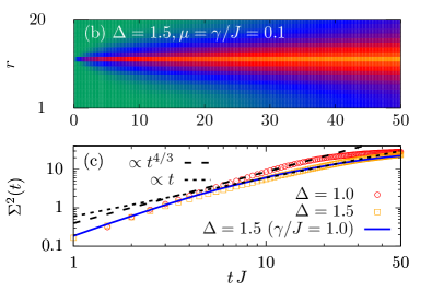
Figure 1: (a) Sketch of our setup. (b) Magnetization dynamics ${\langle S_{r}^{z}(t)\rangle}$ in the spin-1/2 XXZ chain coupled to a single Lindblad bath, obtained from the full stochastic unraveling for anisotropy ${\Delta=1.5}$, small coupling ${\gamma/J=0.1}$, weak driving ${\mu=0.1}$, and ${N=20}$ sites. (c) Corresponding spatial variance $\Sigma^{2}(t)$ for ${\Delta=1.0}$ and ${\Delta=1.5}$. Additionally, a curve for large ${\gamma/J=1.0}$ is depicted for ${\Delta=1.5}$. The dashed (dotted) fits indicate superdiffusive (diffusive) scaling. The saturation of $\Sigma^{2}(t)$ at long times is due to finite $N$.

A canonical approach to quantum transport in closed spin or Hubbard type models is given by linear response theory (LRT) in the form of equilibrium correlation functions [18]. A number of efficient numerical methods have been used to evaluate such correlation functions either in real time or in the frequency domain, including exact diagonalization [35], matrix product state techniques [36, 37], Lanczos methods [38], dynamical quantum typicality [39, 40, 41, 42, 43], semiclassical approximations [44], or quantum Monte Carlo [45].

An alternative approach to transport is to consider an open-system setting, where the model is connected at its ends to reservoirs, which drive a current through the bulk [46, 47, 48, 49]. The time evolution is often described by a Lindblad master equation which induces a nonequilibrium steady state at long times. State-of-the-art algorithms to solve the Lindblad equation are based on a matrix-product-operator formulation, which gives access to huge system sizes, e.g., on the order of hundreds of spin-1/2 degrees of freedom [50, 51, 52, 53, 54]. Especially for systems in the thermodynamic limit, it is expected that the specific form and strength of the system-bath coupling become irrelevant for the steady state. However, the involved Lindblad operators in practice often have to be chosen heuristically. Moreover, extra care has to be taken in the case of finite systems to reproduce the correct behavior of the actual closed system of interest [55]. While agreement between boundary-driven transport and LRT has numerically been observed for selected examples [56, 57], there is no general proof that both approaches need to agree [58, 59, 60, 61, 18], also at weak driving.

In this Letter, we make a significant step forward to bridge the conceptual gap between closed-system and open-system numerical approaches to quantum transport. Focusing on the case of weak driving and relying on typicality and equilibration arguments, we establish a connection between LRT and the finite-time dynamics of an open quantum system in a simple setting introduced below and sketched in Fig. 1(a). Specifically, we unveil that open-system dynamics can be constructed from closed-system correlation functions. This novel connection entails both physical implications regarding the transport properties and consequences regarding efficient numerical simulations of open systems. We also note that Green-Kubo type relations connecting equilibrium correlation functions to open-system transport have been obtained before in classical systems, see e.g., Refs. [58, 62]. We stress that our results and our framework are distinct from such approaches. Rather we provide a means to understand individual trajectories in the unraveling of Lindblad master equations from the dynamics of the closed system.

II Setup

While our theoretical framework applies more generally to other systems, we here demonstrate its validity for the spin-1/2 XXZ chain as a timely example,

$$H=J\sum_{r=1}^{N}(S_{r}^{x}S_{r+1}^{x}+S_{r}^{y}S_{r+1}^{y}+\Delta S_{r}^{z}S_{r+1}^{z})\,,$$ (1)

where $S_{r}^{x,y,z}$ are spin-1/2 operators at site $r$, ${J>0}$ is the antiferromagnetic coupling constant, $\Delta$ denotes the anisotropy in $z$ direction, and $S_{N+1}^{x,y,z}\equiv S_{1}^{x,y,z}$. The high-temperature spin-transport properties of the integrable XXZ chain have been in the focus of intense theoretical and experimental efforts in recent years. While normal diffusion emerges for ${\Delta>1}$ [18], transport is superdiffusive at ${\Delta=1}$ with spatiotemporal correlations following the Kardar-Parisi-Zhang (KPZ) scaling function (see e.g. [28, 37, 63, 64]).

In this Letter, we consider a nonequilibrium situation, where the system of interest is coupled to an external bath, as described by the Lindblad equation

$$\dot{\rho}(t)={\cal L}\,\rho(t)=i[\rho(t),H]+{\cal D}\,\rho(t)\,,$$ (2)

which consists of a coherent time evolution of the density matrix $\rho(t)$ and an incoherent damping term

$${\cal D}\,\rho(t)=\sum_{j}\alpha_{j}\Big{(}L_{j}\rho(t)L_{j}^{\dagger}-\frac{1}{2}\{\rho(t),L_{j}^{\dagger}L_{j}\}\Big{)}\ ,$$ (3)

with non-negative rates $\alpha_{j}$, Lindblad operators $L_{j}$, and the anticommutator $\{\bullet,\bullet\}$. While the derivation of Eqs. (2) and (3) can be a subtle task for a given microscopic model [47, 65] (and might not always be justified [66, 67]), it is the most general form of a time-local quantum master equation, which maps a density matrix to a density matrix [68]. Here, we focus on arguably the simplest possible setup, see Fig. 1(a), where $H$ is coupled to the bath at a single lattice site,

$$L_{1}=S_{r_{0}}^{+}\,,\quad \alpha_{1}=\gamma(1+\mu)\,,$$ (4)

$$L_{2}=L_{1}^{\dagger}=S_{r_{0}}^{-}\,,\quad \alpha_{2}=\gamma(1-\mu)\,,$$ (5)

where $\gamma$ is the system-bath coupling, $\mu$ is the driving strength, and $L_{1}$ and $L_{2}$ are local Lindblad operators at site ${r_{0}=N/2}$. (This site is arbitrary due to periodic boundaries). Note that throughout our work and consistent with the literature on transport [18], we refer to the influence of Lindblad operators as driving. This type of incoherent driving should not be confused with a coherent driving by a time-dependent Hamiltonian.

Considering a homogeneous initial state $\rho(0)$ and choosing $\mu>0$, excess magnetization is induced at the bath site and then transported through the chain. Specifically, we study the time evolution of local densities ${\langle S_{r}^{z}(t)\rangle=\text{tr}[\rho(t)S_{r}^{z}]}$, see Fig. 1(b), which depends on the parameters of the system $H$, but also on the bath parameters $\gamma$ and $\mu$. The emerging transport behavior reflects itself in the growth of the spatial variance [18]

$$\Sigma^{2}(t)=\sum_{r}\frac{\langle S_{r}^{z}(t)\rangle}{\langle S^{z}(t)\rangle}r^{2}-\Big{[}\sum_{r}\frac{\langle S_{r}^{z}(t)\rangle}{\langle S^{z}(t)\rangle}r\Big{]}^{2}\ ,$$ (6)

with ${\langle S^{z}(t)\rangle=\sum_{r}\langle S_{r}^{z}(t)\rangle}$. Importantly, as shown in Fig. 1(c), we find that at weak driving ${\mu=0.1\ll 1}$, the transport behavior of the isolated XXZ chain carries over to the behavior of the open system with diffusive scaling (${\Sigma^{2}(t)\propto t}$) at ${\Delta=1.5}$ and superdiffusive KPZ scaling (${\Sigma^{2}(t)\propto t^{4/3}}$) at ${\Delta=1.0}$. A key contribution of the present work is to show how this result can be understood by connecting the Lindblad setting to the dynamics of correlation functions in the closed system.

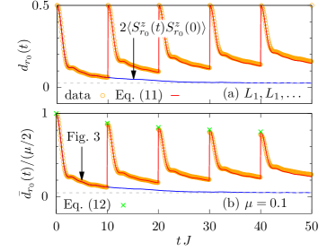
Figure 2: Test setting with artificial jump times $\tau_{k}=0,10,\dots$. (a) Magnetization dynamics $d_{r_{0}}(t)$ at $r_{0}=N/2$ for a single trajectory with Haar-random initial state $|\psi(0)\rangle$ and weak driving ${\mu\ll 1}$. We here consider only the single Lindblad operator $L_{1}$. (b) Average over all possible trajectories with jump operators $L_{1}$ and $L_{2}$, weighted with the respective probabilities for ${\mu=0.1}$. In each case, numerical data (circles) are found to agree convincingly with the prediction in Eqs. (11) (curves) and (12) (crosses). Other parameters: ${\Delta=1.5}$ and ${N=20}$. The dashed line indicates the long-time equilibration value of the correlation function, i.e., $0.5/N$.

III Trajectories and weak Lindblad driving

One possibility to solve the Lindblad equation is given by the concept of stochastic unraveling, which relies on pure states $\ket{\psi}$ rather than density matrices [69, 70]. It consists of an alternating sequence of stochastic jumps and deterministic evolutions with respect to an effective Hamiltonian ${H_{\text{eff}}=H-(i/2)\sum_{j}\alpha_{j}\,L_{j}^{\dagger}L_{j}}$. Given Eqs. (4) and (5), $H_{\text{eff}}$ here takes on the form

$$H_{\text{eff}}=H-\frac{i}{2}\gamma(1+\mu)+i\gamma\mu n_{r_{0}}\approx H-\frac{i}{2}\gamma\,,$$ (7)

where ${n_{r_{0}}=S_{r_{0}}^{+}S_{r_{0}}^{-}=S_{r_{0}}^{z}}+1/2$, and the approximation in the last step applies for weak driving ${\mu\ll 1}$. In particular, for ${\mu\ll 1}$, the deterministic evolution $\exp(-iH_{\text{eff}}t)\ket{\psi(0)}$ simplifies,

$$|\psi(t)\rangle\approx e^{-\gamma t/2}\,e^{-iHt}\,|\psi(0)\rangle\,,$$ (8)

i.e., apart from the scalar damping term, the dynamics is generated by the closed system $H$ only. This simplification will be central to derive our analytical prediction below. However, in our numerical simulations, we always take into account the full expression of $H_{\text{eff}}$ for the stochastic unraveling without approximation.

Since $H_{\text{eff}}$ is non-Hermitian, $\exp(-iH_{\text{eff}}t)\ket{\psi(0)}$ does not conserve the state’s norm. As a consequence, for a given $\varepsilon$ drawn at random from a uniform distribution ${]0,1]}$, there is a time, where the condition ${\left\lVert\psi(t)\rangle\right\rVert^{2}\geq\varepsilon}$ is first violated. At this time, a jump with one of the Lindblad operators occurs, ${\ket{\psi(t)}\to\ket{\psi^{\prime}(t)}=L_{j}|\psi(t)\rangle/\left\lVert L_{j}|\psi(t)\rangle\right\rVert}$, where the specific jump is chosen with probability ${p_{j}=\alpha_{j}\left\lVert L_{j}|\psi(t)\rangle\right\rVert^{2}/\sum_{j^{\prime}}\alpha_{j^{\prime}}\left\lVert L_{j^{\prime}}|\psi(t)\rangle\right\rVert^{2}}$. Thereafter, the next deterministic evolution with respect to $H_{\text{eff}}$ takes place. This sequence of stochastic jumps and deterministic evolutions leads to a particular trajectory. By averaging over trajectories, Eq. (2) can be approximated and expectation values follow as

$$\langle S_{r}^{z}(t)\rangle\approx\frac{1}{\text{T}_{\text{max}}}\sum_{\text{T}=1}^{\text{T}_{\text{max}}}\frac{\langle\psi_{\text{T}}(t)|S_{r}^{z}|\psi_{\text{T}}(t)\rangle}{\left\lVert|\psi_{\text{T}}(t)\rangle\right\rVert^{2}}\,,$$ (9)

where the subscript in $\ket{\psi_{T}(t)}$ labels a random sequence of jumps and deterministic evolutions.

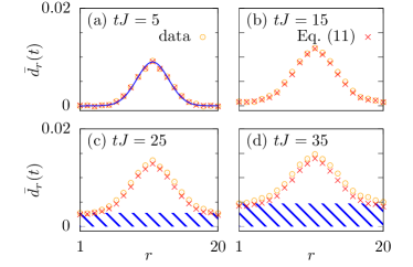
Figure 3: Analogous setup as in Fig. 2(b), but now for the full site dependence $\bar{d}_{r}(t)$ at various fixed times (a)-(d), which all lie in the middle of two jumps. Numerical data (circles) are in convincing agreement with the prediction in Eq. (11) (crosses). A Gaussian is also indicated in (a) for comparison. The striped area indicates the equilibrium background of the already induced magnetization.

IV Dynamical typicality

In a nutshell, quantum typicality asserts that a random pure quantum state can faithfully reproduce properties of the full statistical ensemble [71, 72, 73, 74, 75]. For instance, a homogeneous magnetization distribution at $t=0$, cf. Fig. 1(b), can be readily realized by a Haar-random initial state, $|\psi(0)\rangle=\sum_{j}(a_{j}+ib_{j})\,|\phi_{j}\rangle$, where the coefficients $a_{j}$ and $b_{j}$ in some basis $|\phi_{j}\rangle$ are drawn at random from a Gaussian distribution with zero mean, and $\ket{\psi(0)}$ mimics the maximally mixed state $\rho\propto 1$ [71, 72, 73, 74, 75]. It is further instructive to consider, for the moment, an artificial scenario with a quantum jump immediately at $t=0$, i.e., $|\psi(0)\rangle\to|\psi^{\prime}\rangle\propto L_{1}\ket{\psi(0)}$. This results in a random superposition over a subset of pure states with a spin-up at $r_{0}=N/2$, which mimics ${\rho\propto 1+S_{r_{0}}^{z}}$. Then, the deterministic evolution $d_{r}(t)$ at weak driving, cf. Eq. (8),

$$d_{r}(t)\!\equiv\!\frac{\langle\psi^{\prime}(t)|S_{r}^{z}|\psi^{\prime}(t)\rangle}{\left\lVert|\psi^{\prime}(t)\rangle\right\rVert^{2}}\!\approx\!\langle\psi^{\prime}|e^{iHt}S_{r}^{z}e^{-iHt}|\psi^{\prime}\rangle\,,$$ (10)

can be rewritten as ${d_{r}(t)/2\approx\langle S_{r}^{z}(t)S_{r_{0}}^{z}(0)\rangle}$ via typicality, with ${S_{r}^{z}(t)=e^{iHt}S_{r}^{z}e^{-iHt}}$ and ${\langle\bullet\rangle=\text{tr}[\bullet]/2^{N}}$ denoting the infinite-temperature average [76]. Thus, the dynamics of expectation values $d_{r}(t)$ during the deterministic process are generated by equilibrium correlation functions of the closed system $H$. We numerically demonstrate the validity of this finding in a test setting, where we consider for simplicity only the single jump operator $L_{1}$ and artificially fix the jump times to ${\tau_{k}=k\delta\tau}$ with ${\delta\tau J=10}$. As shown in Fig. 2(a), $\langle S_{r}^{z}(t)S_{r_{0}}^{z}(0)\rangle$ indeed reproduces the deterministic dynamics after the first and before the next jump, $0<t<10$. Furthermore, Fig. 2(a) already highlights that we can actually predict open-system trajectories even with many jumps, which is a main result of this work. As explained in the following, such a description of trajectories with multiple jumps is achieved by superimposing closed-system correlation functions $\langle S_{r}^{z}(t)S_{r_{0}}^{z}(0)\rangle$ appropriately. We should stress that the accuracy of the typicality approximation used so far increases exponentially with $N$ [76].

V Connecting LRT and quantum trajectories

To proceed, we now take into account also the jump operator $L_{2}$, but still use jump times $\tau_{k}=k\delta\tau$ for illustration. Averaging over trajectories weighted according to the jump probabilities of $L_{1}$ and $L_{2}$ with their different prefactors ${\gamma(1+\mu)}$ and ${\gamma(1-\mu)}$, cf. text above Eq. (9), one finds ${\bar{d}_{r}(t)/2=\mu\langle S_{r}^{z}(t)S_{r_{0}}^{z}(0)\rangle}$ for the initial time evolution after the first jump, $0<t<10$, see Fig. 2(b). While this idealized prediction cannot hold exactly at later stages of the trajectory, one can make further progress by assuming a sufficiently small value of $\gamma$. Then, within the deterministic evolution, the system has enough time to equilibrate and expectation values approach ${\bar{d}_{r}(t)/2\to\mu\langle S_{r_{0}}^{z}(0)^{2}\rangle/N}$ [cf. Fig. 2(b)], which approaches zero for large $N$ and thus becomes close to the local magnetizations before the initial jump at $t=0$. Eventually, another jump must occur at some time $\tau$ and, given the above equilibration, a reasonable expectation for the subsequent deterministic evolution is ${\bar{d}_{r}(t)/2=\mu\langle S_{r_{0}}^{z}(0)^{2}\rangle/N+(\mu-\mu/N)\langle S_{r}^{z}(t-\tau)S_{r_{0}}^{z}(0)\rangle}$. Reiterating this procedure, we end up with a prediction for the entire trajectory with jump times $\tau_{k}$,

$$\bar{d}_{r}(t)/2=\mu\sum_{k}A_{k}\,\Theta(t-\tau_{k})\,\langle S_{r}^{z}(t-\tau_{k})S_{r_{0}}^{z}(0)\rangle\,,$$ (11)

where $\Theta$ is the Heavyside function. The amplitudes $A_{k}$ read ${A_{k}/2=1/2-\bar{d}_{r_{0}}(\tau_{k}-0^{+})/\mu}$ and measure the remaining deviation from the long-time equilibrium value, where we implicitly assumed full equilibration towards zero, via the balance ${\left\lVert L_{1}|\psi(t)\rangle\right\rVert^{2}=\left\lVert L_{2}|\psi(t)\rangle\right\rVert^{2}}$. Equation (11) is the central result of this Letter. It predicts that the the open-system dynamics can be described by superimposing closed-system correlation functions at different times. Taking into account also an imbalance, i.e., ${\left\lVert L_{1}|\psi(t)\rangle\right\rVert^{2}\neq\left\lVert L_{2}|\psi(t)\rangle\right\rVert^{2}}$, the $A_{k}$ can be further refined (see Appendix A for details),

$$\!\frac{A_{k}}{2}\!=\!\frac{a_{k}-\bar{d}_{r_{0}}(\tau_{k}-0^{+})}{\mu}\,,\,\,\,a_{k}\!=\!\frac{\mu-2\bar{d}_{r_{0}}(\tau_{k}-0^{+})}{2-4\mu\,\bar{d}_{r_{0}}(\tau_{k}-0^{+})}\,,$$ (12)

with $A_{k}\to 1$ if $\bar{d}_{r_{0}}(\tau_{k}-0^{+})\to 0$. In our numerics, we find Eqs. (11) and (12) to be well fulfilled even if full equilibration is not reached, see Fig. 2(b). Importantly, Eq. (11) not only applies at the bath site $r_{0}=N/2$, but actually describes the full site dependence $\bar{d}_{r}(t)$ accurately, see Fig. 3, albeit with slight deviations at later times.

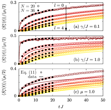
Figure 4: Magnetization dynamics $\langle S_{r}^{z}(t)\rangle$ at different sites $r=r_{0}+l$ (curves), as generated by the full stochastic unraveling procedure (averaged over $10^{5}$ or more trajectories) for ${\Delta=1.5}$ and ${N=20}$. This procedure is performed for the full $H_{\text{eff}}$ without any approximation. (a) Small ${\gamma/J=0.1}$ and (b) strong ${\gamma/J=1.0}$, both for weak ${\mu=0.1}$. (c) Strong ${\mu=1.0}$ and small ${\gamma/J=0.1}$. In all cases, we compare to the prediction (11) for ${N=20}$ and ${N=36}$ (circles).

VI From weak to strong driving

While we have chosen artificial $\tau_{k}$ in Figs. 2 and 3 for illustrative reasons, we now turn to the actual solution of the Lindblad equation. Our analytical prediction for $\langle S_{r}^{z}(t)\rangle$ follows from averaging Eq. (11) over trajectories with random jump times (${\tau_{1},\tau_{2},\ldots\,}$), i.e., ${\langle S_{r}^{z}(t)\rangle\approx(1/\text{T}_{\text{max}})\sum_{\text{T}}\bar{d}_{r,\text{T}}(t)}$. Specifically, given the exponential damping in Eq. (8) for ${\mu\ll 1}$, the $\tau_{k}$ are given by ${\tau_{k+1}=\tau_{k}-\ln\varepsilon/\gamma}$, where a new $\varepsilon$ is drawn at random from ${]0,1]}$ after each jump. Hence, if the correlation function ${\langle S_{r}^{z}(t)S_{r_{0}}^{z}(0)\rangle}$ is known, it is rather straightforward to construct the prediction (11) and the average numerically. Crucially, the computational costs of this procedure are significantly lower compared to the full stochastic unraveling such that we are able to generate dynamics for system sizes ${N=36}$, see Fig. 4 and Appendix B, which is approximately the maximum size reachable for typicality-based calculations of correlation functions. Note, however, that even larger system sizes might be reached when calculating correlation functions from matrix-product state techniques.

In Fig. 4(a)-(c), we summarize our numerical results for $\langle S_{r}^{z}(t)\rangle$, where we consider (i) weak driving ${\mu=0.1}$ and weak coupling ${\gamma/J=0.1}$, (ii) strong coupling ${\gamma/J=1}$, and (iii) strong driving ${\mu=1}$. We compare our prediction to the numerically exact stochastic unraveling which is performed for the full $H_{\text{eff}}$ and a homogeneous initial state. We find that the prediction and the exact dynamics agree perfectly for (i), while the agreement becomes worse for (ii) and (iii), as expected. The convincing agreement in Fig. 4(a) confirms our initial observation that the transport behavior of the closed system carries over to the open system (cf. Fig. 1). Specifically, superpositions of correlation functions with diffusive (superdiffusive) scaling at ${\Delta=1.5}$ (${\Delta=1}$) according to Eq. (11) yield a dynamics with the same scaling, see also Appendix D.

VII Conclusion

In summary, we have studied nonequilibrium dynamics and transport in spin chains with a local coupling to a Lindblad bath. For weak driving, we have unveiled that the open-system dynamics can be constructed on the basis of closed-system correlation functions, which establishes a connection between LRT and the Lindblad setting. For this specific setting, from a conceptual point of view, our results confirm the common assumption that closed-system and open-system approaches to transport should agree if the relevant parameters are chosen appropriately. From a practical point of view, our framework sheds new light on the efficient stochastic unravelings of Lindblad equations for large system sizes and long time scales. While we have chosen the XXZ chain as a timely example, our framework can be applied also to other spin or Hubbard models.

Promising directions of future research are, e.g., the generalization of our results to boundary-driven situations with a bath at each end of the system, which seems to be feasible [77]. Another interesting avenue is to study the role of integrability in more detail. In particular, our finding of persisting superdiffusive transport even in the presence of a system-bath coupling appears related to recent works that explored effect of weak integrability-breaking perturbations [78, 79].

Appendix A Amplitudes

One possibility to derive the amplitudes in Eq. (12) is based on typicality arguments. To this end, consider a maximally random pure state ${|\psi(\tau_{j}-0^{+})\rangle}$ under the constraint

$$d_{r_{0}}(\tau_{j}-0^{+})=x\,,$$ (13)

before a jump occurs at time $\tau_{j}$. Then, we have

$$y_{1}=\left\lVert L_{1}|\psi(\tau_{j}-0^{+})\rangle\right\rVert^{2}=\frac{1}{2}-x$$ (14)

and

$$y_{2}=\left\lVert L_{2}|\psi(\tau_{j}-0^{+})\rangle\right\rVert^{2}=x+\frac{1}{2}$$ (15)

with ${y_{1}+y_{2}=1}$. The corresponding jump probabilities read

$$p_{1}=\frac{(1+\mu)y_{1}}{(1+\mu)y_{1}+(1-\mu)y_{2}}$$ (16)

and

$$p_{2}=\frac{(1-\mu)y_{2}}{(1-\mu)y_{2}+(1+\mu)y_{1}}$$ (17)

with ${p_{1}+p_{2}=1}$ again. Consequently, a straightforward calculation yields

$$\frac{p_{1}}{2}-\frac{p_{2}}{2}=\frac{\mu-2x}{2-4\mu x}\,,$$ (18)

i.e., the expression in Eq. (12).

Appendix B Dependence on $\gamma$ and $N$

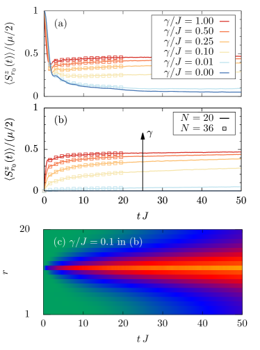
Figure 5: Time evolution of the magnetization ${\langle S_{r_{0}}^{z}(t)\rangle}$ at the position $r_{0}=N/2$ of the local Lindblad operators, as given for weak driving ${\mu=0.1}$ by Eq. (11) with amplitudes according to Eq. (12). Curves for various values of the bath coupling $\gamma$ are obtained from the average over 10,000 different trajectories. The other model parameters are the same as in Figs. 2 and 3. A bath coupling ${\gamma/J=0.1}$ is comparable to the jump times in Fig. 2. (a) and (b) correspond to an initial state with and without local magnetization, respectively. In each case, data for ${N=36}$ sites is also depicted. (c) Full site dependence for ${\gamma/J=0.1}$ in (b).

Since we have mostly discussed the case of a small bath coupling ${\gamma/J=0.1}$, we depict in Fig. 5 the prediction according to Eq. (11) for various values of $\gamma$. We do so for the magnetization ${\langle S_{r_{0}}^{z}(t)\rangle}$ at the position $r_{0}=N/2$ of the local Lindblad operators and random initial states ${|\psi(0)\rangle}$ with and without local magnetization. Moreover, to demonstrate that this prediction does not depend on system size, we also show the corresponding prediction for ${N=36}$ sites.

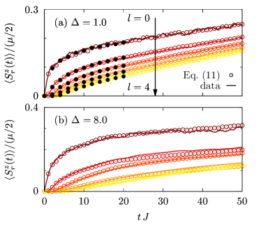
Figure 6: Dynamics of the magnetization $\langle S_{r}^{z}(t)\rangle$ at various sites ${r=r_{0}+l}$ for anisotropies (a) ${\Delta=1.0}$ and (b) ${\Delta=8.0}$, as generated by the full stochastic unraveling procedure and as predicted by Eq. (11). Remaining model parameters: Small coupling ${\gamma/J=0.1}$, weak driving ${\mu=0.1}$, and system size ${N=20}$.

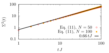
Figure 7: Time-dependent spatial variance $\Sigma^{2}(t)$, as predicted by Eq. (11) for ${D_{\text{closed}}/J=0.6}$.

Appendix C Other anisotropies

In Fig. 4, we have provided a detailed comparison of the dynamics for anisotropy ${\Delta=1.5}$, as generated by the full stochastic unraveling procedure and as predicted by Eq. (11). To demonstrate that an agreement of similar quality can be obtained for other anisotropies as well, we show in Fig. 6 a comparison for ${\Delta=1.0}$ and ${\Delta=8.0}$, in both cases for small coupling ${\gamma/J=0.1}$ and weak driving ${\mu=0.1}$.

Appendix D Diffusion coefficient

Let us, for simplicity, estimate the expansion velocity of the open system by

$$\frac{v_{\text{open}}}{D_{\text{closed}}}=\frac{D_{\text{closed}}(t-\bar{\tau})}{D_{\text{closed}}\,t}$$ (19)

with the average injection time

$$\bar{\tau}=-\frac{1}{\gamma}\int_{0^{+}}^{1}\text{d}\varepsilon\,\ln\varepsilon\,,$$ (20)

which is ${\bar{\tau}J\approx 10}$ for ${\gamma/J=0.1}$. By taking into account ${D_{\text{closed}}/J\approx 0.6}$ for ${\Delta=1.5}$, one would expect at ${t=2\bar{\tau}}$ the expansion velocity

$$\frac{v_{\text{open}}}{J}\approx\frac{0.6}{2}=0.3\,.$$ (21)

Thus, a reasonable expectation is

$$\Sigma^{2}(t)=2\,v_{\text{open}}t\approx 0.6\,tJ\,.$$ (22)

And indeed, this number is chosen as the prefactor of the power law in Fig. 1.

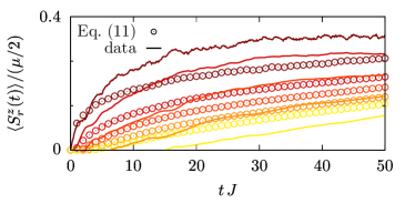
Figure 8: Analogous comparison as the one in Fig. 4(a), but now the initial pure state ${|\psi(0)\rangle}$ is not drawn at random.

An alternative and kind of better way to estimate the expansion velocity in the open system is provided by Eq. (11) and the assumption of perfectly diffusive behavior in the closed system (with a zero mean free path). Then, the equilibrium correlation functions take on the simple form

$$\langle S_{r}^{z}(t)S_{r_{0}}^{z}(0)\rangle=\frac{1}{4}\,\exp(-2D_{\text{closed}}t)\,{\cal I}_{r}(2D_{\text{closed}}t)\,,$$ (23)

where ${\cal I}_{r}(t)$ is the modified Bessel function of the first kind and of the order $r$. By the use of this assumption, the calculation of the time-dependent variance $\Sigma^{2}(t)$ in the open system can be done numerically. As depicted in Fig. 7 for ${D_{\text{closed}}/J=0.6}$, one finds

$$\Sigma^{2}(t)\approx 0.66\,tJ$$ (24)

over a wide range of time, which is consistent with the simple argument above. Note that the calculation can be easily carried out for ${N=100}$ of lattice sites.

Appendix E Other initial states

The derivation of the prediction in Eq. (11) has relied on an initial pure state ${|\psi(0)\rangle}$, which is fully random and corresponds to an equilibrium density matrix at formally infinite temperature. In Fig. 8, we demonstrate that this prediction does not apply to other initial states. To this end, we choose the specific initial pure state

$$|\psi(0)\rangle\propto(|\!\uparrow\rangle+|\!\downarrow\rangle)\otimes\ldots\otimes(|\!\uparrow\rangle+|\!\downarrow\rangle)\,,$$ (25)

which is known to be untypical.

References

- Polkovnikov et al. [2011] A. Polkovnikov, K. Sengupta, A. Silva, and M. Vengalattore, Colloquium : Nonequilibrium dynamics of closed interacting quantum systems, Rev. Mod. Phys. 83, 863 (2011).
- Nandkishore and Huse [2015] R. M. Nandkishore and D. A. Huse, Many-Body Localization and Thermalization in Quantum Statistical Mechanics, Annu. Rev. Condens. Matter Phys. 6, 15 (2015).
- D’Alessio et al. [2016] L. D’Alessio, Y. Kafri, A. Polkovnikov, and M. Rigol, From quantum chaos and eigenstate thermalization to statistical mechanics and thermodynamics, Adv. Phys. 65, 239 (2016).
- Khemani et al. [2018] V. Khemani, A. Vishwanath, and D. A. Huse, Operator Spreading and the Emergence of Dissipative Hydrodynamics under Unitary Evolution with Conservation Laws, Phys. Rev. X 8, 031057 (2018).
- Rakovszky et al. [2018] T. Rakovszky, F. Pollmann, and C. W. von Keyserlingk, Diffusive Hydrodynamics of Out-of-Time-Ordered Correlators with Charge Conservation, Phys. Rev. X 8, 031058 (2018).
- Abanin et al. [2019] D. A. Abanin, E. Altman, I. Bloch, and M. Serbyn, Colloquium : Many-body localization, thermalization, and entanglement, Rev. Mod. Phys. 91, 021001 (2019).
- Serbyn et al. [2021] M. Serbyn, D. A. Abanin, and Z. Papić, Quantum many-body scars and weak breaking of ergodicity, Nat. Phys. 17, 675 (2021).
- Dziarmaga [2010] J. Dziarmaga, Dynamics of a quantum phase transition and relaxation to a steady state, Adv. Phys. 59, 1063 (2010).
- Sieberer et al. [2013] L. M. Sieberer, S. D. Huber, E. Altman, and S. Diehl, Dynamical Critical Phenomena in Driven-Dissipative Systems, Phys. Rev. Lett. 110, 195301 (2013).
- Prüfer et al. [2018] M. Prüfer, P. Kunkel, H. Strobel, S. Lannig, D. Linnemann, C.-M. Schmied, J. Berges, T. Gasenzer, and M. K. Oberthaler, Observation of universal dynamics in a spinor Bose gas far from equilibrium, Nature 563, 217 (2018).
- Erne et al. [2018] S. Erne, R. Bücker, T. Gasenzer, J. Berges, and J. Schmiedmayer, Universal dynamics in an isolated one-dimensional Bose gas far from equilibrium, Nature 563, 225 (2018).
- Rodriguez-Nieva et al. [2022] J. F. Rodriguez-Nieva, A. Piñeiro Orioli, and J. Marino, Far-from-equilibrium universality in the two-dimensional Heisenberg model. Proc. Natl. Acad. Sci. U.S.A. 119, e2122599119 (2022).
- Kaufman et al. [2016] A. M. Kaufman, M. E. Tai, A. Lukin, M. Rispoli, R. Schittko, P. M. Preiss, and M. Greiner, Quantum thermalization through entanglement in an isolated many-body system, Science 353, 794 (2016).
- Lüschen et al. [2017] H. P. Lüschen, P. Bordia, S. S. Hodgman, M. Schreiber, S. Sarkar, A. J. Daley, M. H. Fischer, E. Altman, I. Bloch, and U. Schneider, Signatures of Many-Body Localization in a Controlled Open Quantum System, Phys. Rev. X 7, 011034 (2017).
- Rubio-Abadal et al. [2019] A. Rubio-Abadal, J.-y. Choi, J. Zeiher, S. Hollerith, J. Rui, I. Bloch, and C. Gross, Many-Body Delocalization in the Presence of a Quantum Bath, Phys. Rev. X 9, 041014 (2019).
- Diehl et al. [2008] S. Diehl, A. Micheli, A. Kantian, B. Kraus, H. P. Büchler, and P. Zoller, Quantum states and phases in driven open quantum systems with cold atoms, Nat. Phys. 4, 878 (2008).
- Weimer et al. [2010] H. Weimer, M. Müller, I. Lesanovsky, P. Zoller, and H. P. Büchler, A Rydberg quantum simulator, Nat. Phys. 6, 382 (2010).
- Bertini et al. [2021] B. Bertini, F. Heidrich-Meisner, C. Karrasch, T. Prosen, R. Steinigeweg, and M. Žnidarič, Finite-temperature transport in one-dimensional quantum lattice models, Rev. Mod. Phys. 93, 025003 (2021).
- Lux et al. [2014] J. Lux, J. Müller, A. Mitra, and A. Rosch, Hydrodynamic long-time tails after a quantum quench, Phys. Rev. A 89, 053608 (2014).
- Bohrdt et al. [2017] A. Bohrdt, C. B. Mendl, M. Endres, and M. Knap, Scrambling and thermalization in a diffusive quantum many-body system, New J. Phys. 19, 063001 (2017).
- Richter et al. [2018] J. Richter, F. Jin, H. De Raedt, K. Michielsen, J. Gemmer, and R. Steinigeweg, Real-time dynamics of typical and untypical states in nonintegrable systems, Phys. Rev. B 97, 174430 (2018).
- Kloss and Bar Lev [2019] B. Kloss and Y. Bar Lev, Spin transport in a long-range-interacting spin chain, Phys. Rev. A 99, 032114 (2019).
- Schuckert et al. [2020] A. Schuckert, I. Lovas, and M. Knap, Nonlocal emergent hydrodynamics in a long-range quantum spin system, Phys. Rev. B 101, 020416(R) (2020).
- Richter et al. [2023] J. Richter, O. Lunt, and A. Pal, Transport and entanglement growth in long-range random Clifford circuits, Phys. Rev. Research 5, L012031 (2023).
- Luitz and Lev [2017] D. J. Luitz and Y. B. Lev, The ergodic side of the many‐body localization transition, Ann. Phys. 529, 1600350 (2017).
- Richter and Pal [2022] J. Richter and A. Pal, Anomalous hydrodynamics in a class of scarred frustration-free Hamiltonians, Phys. Rev. Research 4, L012003 (2022).
- Singh et al. [2021] H. Singh, B. A. Ware, R. Vasseur, and A. J. Friedman, Subdiffusion and Many-Body Quantum Chaos with Kinetic Constraints, Phys. Rev. Lett. 127, 230602 (2021).
- Bulchandani et al. [2021] V. B. Bulchandani, S. Gopalakrishnan, and E. Ilievski, Superdiffusion in spin chains, J. Stat. Mech. 2021, 084001 (2021).
- Bertini et al. [2016] B. Bertini, M. Collura, J. De Nardis, and M. Fagotti, Transport in Out-of-Equilibrium XXZ Chains: Exact Profiles of Charges and Currents, Phys. Rev. Lett. 117, 207201 (2016).
- Castro-Alvaredo et al. [2016] O. A. Castro-Alvaredo, B. Doyon, and T. Yoshimura, Emergent Hydrodynamics in Integrable Quantum Systems Out of Equilibrium, Phys. Rev. X 6, 041065 (2016).
- [31] E. Leviatan, F. Pollmann, J. H. Bardarson, D. A. Huse, and E. Altman, Quantum thermalization dynamics with Matrix-Product States, arXiv:1702.08894 .
- Ye et al. [2020] B. Ye, F. Machado, C. D. White, R. S. K. Mong, and N. Y. Yao, Emergent Hydrodynamics in Nonequilibrium Quantum Systems, Phys. Rev. Lett. 125, 030601 (2020).
- White et al. [2018] C. D. White, M. Zaletel, R. S. K. Mong, and G. Refael, Quantum dynamics of thermalizing systems, Phys. Rev. B 97, 035127 (2018).
- Rakovszky et al. [2022] T. Rakovszky, C. W. von Keyserlingk, and F. Pollmann, Dissipation-assisted operator evolution method for capturing hydrodynamic transport, Phys. Rev. B 105, 075131 (2022).
- Heidrich-Meisner et al. [2007] F. Heidrich-Meisner, A. Honecker, and W. Brenig, Transport in quasi one-dimensional spin-1/2 systems, Eur. Phys. J. Spec. Top. 151, 135 (2007).
- Karrasch et al. [2012] C. Karrasch, J. H. Bardarson, and J. E. Moore, Finite-Temperature Dynamical Density Matrix Renormalization Group and the Drude Weight of Spin-1/2 Chains, Phys. Rev. Lett. 108, 227206 (2012).
- Ljubotina et al. [2017] M. Ljubotina, M. Žnidarič, and T. Prosen, Spin diffusion from an inhomogeneous quench in an integrable system, Nat. Commun. 8, 16117 (2017).
- Long et al. [2003] M. W. Long, P. Prelovšek, S. El Shawish, J. Karadamoglou, and X. Zotos, Finite-temperature dynamical correlations using the microcanonical ensemble and the Lanczos algorithm, Phys. Rev. B 68, 235106 (2003).
- Steinigeweg et al. [2014] R. Steinigeweg, J. Gemmer, and W. Brenig, Spin-Current Autocorrelations from Single Pure-State Propagation, Phys. Rev. Lett. 112, 120601 (2014).
- Elsayed and Fine [2013] T. A. Elsayed and B. V. Fine, Regression Relation for Pure Quantum States and Its Implications for Efficient Computing, Phys. Rev. Lett. 110, 070404 (2013).
- Richter and Steinigeweg [2019] J. Richter and R. Steinigeweg, Combining dynamical quantum typicality and numerical linked cluster expansions, Phys. Rev. B 99, 094419 (2019).
- Heitmann et al. [2020] T. Heitmann, J. Richter, D. Schubert, and R. Steinigeweg, Selected applications of typicality to real-time dynamics of quantum many-body systems, Z. Naturforsch. A 75, 421 (2020).
- Jin et al. [2021] F. Jin, D. Willsch, M. Willsch, H. Lagemann, K. Michielsen, and H. De Raedt, Random State Technology, J. Phys. Soc. Jpn. 90, 012001 (2021).
- Wurtz et al. [2018] J. Wurtz, A. Polkovnikov, and D. Sels, Cluster truncated Wigner approximation in strongly interacting systems, Ann. Phys. (NY) 395, 341 (2018).
- Grossjohann and Brenig [2010] S. Grossjohann and W. Brenig, Hydrodynamic limit for the spin dynamics of the Heisenberg chain from quantum Monte Carlo calculations, Phys. Rev. B 81, 012404 (2010).
- Michel et al. [2003] M. Michel, M. Hartmann, J. Gemmer, and G. Mahler, Fourier’s Law confirmed for a class of small quantum systems, Eur. Phys. J. B 34, 325 (2003).
- Wichterich et al. [2007] H. Wichterich, M. J. Henrich, H.-P. Breuer, J. Gemmer, and M. Michel, Modeling heat transport through completely positive maps, Phys. Rev. E 76, 031115 (2007).
- Žnidarič [2011] M. Žnidarič, Spin Transport in a One-Dimensional Anisotropic Heisenberg Model, Phys. Rev. Lett. 106, 220601 (2011).
- Žnidarič et al. [2016] M. Žnidarič, A. Scardicchio, and V. K. Varma, Diffusive and Subdiffusive Spin Transport in the Ergodic Phase of a Many-Body Localizable System, Phys. Rev. Lett. 117, 040601 (2016).
- Prosen and Žnidarič [2009] T. Prosen and M. Žnidarič, Matrix product simulations of non-equilibrium steady states of quantum spin chains, J. Stat. Mech. 2009, P02035 (2009).
- Verstraete et al. [2004] F. Verstraete, J. J. García-Ripoll, and J. I. Cirac, Matrix Product Density Operators: Simulation of Finite-Temperature and Dissipative Systems, Phys. Rev. Lett. 93, 207204 (2004).
- Zwolak and Vidal [2004] M. Zwolak and G. Vidal, Mixed-State Dynamics in One-Dimensional Quantum Lattice Systems: A Time-Dependent Superoperator Renormalization Algorithm, Phys. Rev. Lett. 93, 207205 (2004).
- Weimer et al. [2021] H. Weimer, A. Kshetrimayum, and R. Orús, Simulation methods for open quantum many-body systems, Rev. Mod. Phys. 93, 015008 (2021).
- Lenarčič et al. [2020] Z. Lenarčič, O. Alberton, A. Rosch, and E. Altman, Critical Behavior near the Many-Body Localization Transition in Driven Open Systems, Phys. Rev. Lett. 125, 116601 (2020).
- Prelovšek et al. [2022] P. Prelovšek, S. Nandy, Z. Lenarčič, M. Mierzejewski, and J. Herbrych, From dissipationless to normal diffusion in the easy-axis Heisenberg spin chain, Phys. Rev. B 106, 245104 (2022).
- Steinigeweg et al. [2009] R. Steinigeweg, M. Ogiewa, and J. Gemmer, Equivalence of transport coefficients in bath-induced and dynamical scenarios, EPL (Europhys. Lett.) 87, 10002 (2009).
- Žnidarič and Ljubotina [2018] M. Žnidarič and M. Ljubotina, Interaction instability of localization in quasiperiodic systems, Proc. Natl. Acad. Sci. U.S.A. 115, 4595 (2018).
- Kundu et al. [2009] A. Kundu, A. Dhar, and O. Narayan, The Green–Kubo formula for heat conduction in open systems, J. Stat. Mech. 2009, L03001 (2009).
- Purkayastha et al. [2018] A. Purkayastha, S. Sanyal, A. Dhar, and M. Kulkarni, Anomalous transport in the Aubry-André-Harper model in isolated and open systems, Phys. Rev. B 97, 174206 (2018).
- Purkayastha [2019] A. Purkayastha, Classifying transport behavior via current fluctuations in open quantum systems, J. Stat. Mech. 2019, 043101 (2019).
- Žnidarič [2019] M. Žnidarič, Nonequilibrium steady-state Kubo formula: Equality of transport coefficients, Phys. Rev. B 99, 035143 (2019).
- Dhar [2008] A. Dhar, Heat transport in low-dimensional systems, Advances in Physics 57, 457 (2008).
- Ljubotina et al. [2019] M. Ljubotina, M. Žnidarič, and T. Prosen, Kardar-Parisi-Zhang Physics in the Quantum Heisenberg Magnet, Phys. Rev. Lett. 122, 210602 (2019).
- Gopalakrishnan and Vasseur [2019] S. Gopalakrishnan and R. Vasseur, Kinetic Theory of Spin Diffusion and Superdiffusion in XXZ Spin Chains, Phys. Rev. Lett. 122, 127202 (2019).
- De Raedt et al. [2017] H. De Raedt, F. Jin, M. I. Katsnelson, and K. Michielsen, Relaxation, thermalization, and Markovian dynamics of two spins coupled to a spin bath, Phys. Rev. E 96, 053306 (2017).
- Thingna et al. [2013] J. Thingna, J.-S. Wang, and P. Hänggi, Reduced density matrix for nonequilibrium steady states: A modified Redfield solution approach, Phys. Rev. E 88, 052127 (2013).
- Tupkary et al. [2022] D. Tupkary, A. Dhar, M. Kulkarni, and A. Purkayastha, Fundamental limitations in Lindblad descriptions of systems weakly coupled to baths, Phys. Rev. A 105, 032208 (2022).
- Breuer and Petruccione [2007] H.-P. Breuer and F. Petruccione, The Theory of Open Quantum Systems (Oxford University Press, 2007).
- Dalibard et al. [1992] J. Dalibard, Y. Castin, and K. Mølmer, Wave-function approach to dissipative processes in quantum optics, Phys. Rev. Lett. 68, 580 (1992).
- Michel et al. [2008] M. Michel, O. Hess, H. Wichterich, and J. Gemmer, Transport in open spin chains: A Monte Carlo wave-function approach, Phys. Rev. B 77, 104303 (2008).
- Gemmer et al. [2004] J. Gemmer, M. Michel, and G. Mahler, Quantum Thermodynamics, Lecture Notes in Physics, Vol. 657 (Springer Berlin Heidelberg, 2004).
- Goldstein et al. [2006] S. Goldstein, J. L. Lebowitz, R. Tumulka, and N. Zanghì, Canonical Typicality, Phys. Rev. Lett. 96, 050403 (2006).
- Popescu et al. [2006] S. Popescu, A. J. Short, and A. Winter, Entanglement and the foundations of statistical mechanics, Nat. Phys. 2, 754 (2006).
- Reimann [2007] P. Reimann, Typicality for Generalized Microcanonical Ensembles, Phys. Rev. Lett. 99, 160404 (2007).
- Bartsch and Gemmer [2009] C. Bartsch and J. Gemmer, Dynamical Typicality of Quantum Expectation Values, Phys. Rev. Lett. 102, 110403 (2009).
- Steinigeweg et al. [2017] R. Steinigeweg, F. Jin, D. Schmidtke, H. De Raedt, K. Michielsen, and J. Gemmer, Real-time broadening of nonequilibrium density profiles and the role of the specific initial-state realization, Phys. Rev. B 95, 035155 (2017).
- [77] T. Heitmann, J. Richter, F. Jin, S. Nandy, Z. Lenarčič, J. Herbrych, K. Michielsen, H. De Raedt, J. Gemmer, and R. Steinigeweg, The spin-1/2 xxz chain coupled to two lindblad baths: Constructing nonequilibrium steady states from equilibrium correlation functions, arXiv:2303.00430 .
- De Nardis et al. [2021] J. De Nardis, S. Gopalakrishnan, R. Vasseur, and B. Ware, Stability of Superdiffusion in Nearly Integrable Spin Chains, Phys. Rev. Lett. 127, 057201 (2021).
- Wei et al. [2022] D. Wei, A. Rubio-Abadal, B. Ye, F. Machado, J. Kemp, K. Srakaew, S. Hollerith, J. Rui, S. Gopalakrishnan, N. Y. Yao, I. Bloch, and J. Zeiher, Quantum gas microscopy of Kardar-Parisi-Zhang superdiffusion, Science 376, 716 (2022).