Channel-driven Decentralized Bayesian Federated Learning for trustworthy decision making in D2D Networks

Abstract

Bayesian Federated Learning (FL) offers a principled framework to account for the uncertainty caused by limitations in the data available at the nodes implementing collaborative training. In Bayesian FL, nodes exchange information about local posterior distributions over the model parameters space. This paper focuses on Bayesian FL implemented in a device-to-device (D2D) network via Decentralized Stochastic Gradient Langevin Dynamics (DSGLD), a recently introduced gradient-based Markov Chain Monte Carlo (MCMC) method. Based on the observation that DSGLD applies random Gaussian perturbations of model parameters, we propose to leverage channel noise on the D2D links as a mechanism for MCMC sampling. The proposed approach is compared against a conventional implementation of frequentist FL based on compression and digital transmission, highlighting advantages and limitations.

Index Terms—  Federated Learning, Markov Chain Monte Carlo, Bayesian inference, Decentralized networks

1 Introduction

Federated Learning (FL) enables the collaborative training of Machine Learning (ML) models without the direct exchange of data in both star and fully decentralized architectures [1, 2, 3]. FL is particularly useful when the participating nodes have limited data. This is the case, for instance, in vehicular applications in which individual vehicles can only sense part of a scene (see Fig. 1) [4]. When data sets are size limited, the classical, frequentist, implementation of FL is known to produce models that fail to properly account for the uncertainty of their decisions [5]. This is an important issue for safety-critical applications, such as in automated driving services that require trustworthy decisions even in situations with limited data. A well-established solution to this problem is to implement Bayesian learning, which encodes uncertainty in the posterior distribution of the model parameters (see, e.g., [5]). However, a federated implementation of Bayesian learning poses challenges related to the overhead of communicating information about model distributions [6, 7].

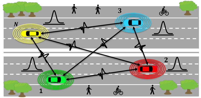
Fig. 1: In the decentralized FL set-up under study, nodes (here $N=4$) implement Bayesian learning via Decentralized Stochastic Gradient Langevin Dynamics (DSGLD) by levearging noise on inter-agent communications for sampling.

In a centralized setting, Bayesian learning is practically implemented via approximate methods relying on variational inference (VI) [8] or Markov Chain Monte Carlo (MCMC), with the latter representing the target posterior distribution via random samples [9, 5]. Distributed implementations of Bayesian learning have been emerging for both star and device-to-device (D2D) topologies adopting VI [10, 6] or MCMC [11, 12], while assuming ideal communication links. In this paper, we propose a new MCMC-based Bayesian FL system tailored for wireless D2D networks with noisy links subject to mutual interference.

To this end, we focus on Stochastic Gradient Langevin Dynamics (SGLD) [13], an MCMC scheme that has the practical advantage of requiring minor modifications as compared to standard frequentist methods. In fact, SGLD is based on the application of Gaussian perturbations to model parameters updated via gradient descent. Reference [14] introduced a federated implementation of SGLD over a wireless star, i.e., base station-centric, topology. The work [14] argued that channel noise between devices and base station can be repurposed to serve as sampling noise for the SGLD updates, an approach referred to as channel-driven sampling. In this paper, we draw inspiration from [14] and study implementations of SGLD in a D2D architecture, as depicted in Fig. 1. We specifically consider the Decentralized Stochastic Gradient Langevin Dynamics (DSGLD) algorithm introduced in [12] under the assumption of noiseless communications, and we propose an analog communication-based implementation that leverages channel-driven sampling and over-the-air computing [15, 16, 17]. Non-orthogonal multiple access to a shared channel is exploited for over-the-air model aggregation, enabling an efficient FL implementation. Experiments focus on a challenging automotive use case where vehicles collaboratively train a Deep Neural Network (DNN) for lidar sensing. Numerical results show that the proposed method is able to provide well-calibrated DNN models that support trustworthy predictions even when a conventional frequentist FL approach based on digital communication fails to meet calibration requirements.

The remainder of this paper is organized as follows. Sec. 2 describes the system model, and Sec. 3 reviews DSGLD. Sec. 4 presents the proposed channel-driven method for Bayesian FL, while Sec. 5 details the numerical results. Finally, Sec. 6 draws some conclusions.

2 System model

We consider the decentralized FL system in Fig. 1, which consists of $N$ agents connected according to the undirected graph $\mathcal{G}=(\mathcal{N},\mathcal{E})$, where $\mathcal{N}=\{1,\ldots,N\}$ is the set of all devices and $\mathcal{E}$ is the set of the directed edges. We denote as $\mathcal{N}_{k}$ the set of neighbors of node $k$ including $k$, while $\mathcal{N}_{\overline{k}}$ is the same subset excluding node $k$. Each agent has access to a local dataset $\mathcal{D}_{k}=\{(\mathbf{d}_{h},\ell_{h})\}_{h=1}^{E_{k}}$ comprising $E_{k}$ training examples, where $\mathbf{d}_{h}$ and $\ell_{h}$ are the input data and the corresponding desired output, or label, respectively. Considering all agents, we have the global dataset $\mathcal{D}=\{\mathcal{D}_{k}\}_{k=1}^{N}$. The goal of the system is to implement Bayesian learning via gradient-based MCMC to obtain a set of samples $\boldsymbol{\theta}\in\mathbb{R}^{m}$ approximating the true global posterior $p(\boldsymbol{\theta}|\mathcal{D})$ of the model $\boldsymbol{\theta}$ learned cooperatively by all agents. This objective should be met by relying only on local computations at the agents and on D2D communications among the agents. The posterior distribution $p(\boldsymbol{\theta}|\mathcal{D})$ describes the uncertainty of the learned model, identifying a set of potential models and the related probabilities.

The agents communicate over full-duplex shared wireless channels impaired by Additive White Gaussian Noise (AWGN). Communication is organized into blocks, each consisting of $m$ channel uses. In each block $s=1,2,\ldots$ the $m$-sample signal received by agent $k$ can be expressed as

$$\mathbf{y}_{k}^{[s]}=\sum_{j\in\mathcal{N}_{\overline{k}}}\mathbf{x}_{j}^{[s]}+\mathbf{z}_{k}^{[s]}\,,$$ (1)

where $\mathbf{z}_{k}^{[s]}\sim\mathcal{N}(0,N_{0}\mathbf{I}_{m})$ is the channel noise ($\mathbf{I}_{m}$ is the $m\times m$ identity matrix), and the $m$-sample block $\mathbf{x}_{j}^{[s]}$ transmitted by each node $j$ satisfies the power constraint $\|\mathbf{x}_{j}^{[s]}\|^{2}\leq mP$.

3 Distributed Stochastic Gradient Langevin Dynamics

In this section, we review DSGLD [12], which applies to a system with ideal inter-agent communication.

3.1 Centralized Stochastic Gradient Langevin Dynamics

We start by reviewing the standard SGLD scheme [13], which applies in the ideal case where the global data set $\mathcal{D}$ is available at a central processor. Given a likelihood function $p(\mathcal{D}_{k}|\boldsymbol{\theta})$ describing the shared ML model adopted by the agents (e.g., a neural network), and a prior distribution $p(\boldsymbol{\theta})$, the global posterior distribution is defined as

$$p(\boldsymbol{\theta}|\mathcal{D})\propto p(\boldsymbol{\theta})\prod_{k=1}^{N}p(\mathcal{D}_{k}|\boldsymbol{\theta})\,,$$ (2)

with $p(\mathcal{D}_{k}|\boldsymbol{\theta})=\prod_{h=1}^{E_{k}}p(\ell_{h}|\mathbf{d}_{h},\boldsymbol{\theta})$. SGLD produces samples whose asymptotic distribution approximately matches the global posterior $p(\boldsymbol{\theta}|\mathcal{D})$.

This is accomplished by adding Gaussian noise to standard gradient descent updates via the following iterative update rule [13]

$$\boldsymbol{\theta}^{[s+1]}=\boldsymbol{\theta}^{[s]}-\eta\nabla f(\boldsymbol{\theta}^{[s]})+\sqrt{2\eta}\boldsymbol{\xi}^{[s+1]}\,,$$ (3)

where $s=1,2,\ldots;$ $\eta$ is the step size; $f(\boldsymbol{\theta})=\sum_{k=1}^{N}f_{k}(\boldsymbol{\theta})$ is the negative logarithm of the unnormalized global posterior $p(\boldsymbol{\theta})\prod_{k=1}^{N}p(\mathcal{D}_{k}|\boldsymbol{\theta})$, with

$$f_{k}(\boldsymbol{\theta})=-\log p(\mathcal{D}_{k}|\boldsymbol{\theta})-\dfrac{1}{N}\log p(\boldsymbol{\theta})\,,$$ (4)

and $\boldsymbol{\xi}^{[s+1]}$ is a sequence of identical and independent (i.i.d.) random vectors following the Gaussian distribution $\mathcal{N}(0,\mathbf{I}_{m})$, independent of the initialization $\boldsymbol{\theta}^{[0]}\in\mathbb{R}^{m}$.

3.2 Decentralized Stochastic Gradient Langevin Dynamics

DSGLD [12] is an extension of SGLD that applies to D2D networks. In DSGLD, each agent $k$ applies the following update rule

$$\boldsymbol{\theta}_{k}^{[s+1]}=\sum_{j\in\mathcal{N}_{k}}w_{kj}\boldsymbol{\theta}_{j}^{[s]}-\eta\nabla f_{k}(\boldsymbol{\theta}_{k}^{[s]})+\sqrt{2\eta}\boldsymbol{\xi}_{k}^{[s+1]}\,,$$ (5)

where $w_{kj}$ is the $(k,j)$-th entry of a symmetric, doubly stochastic matrix $\mathbf{W}$. Accordingly, in DSGLD, at each iteration $s$, each agent $k$ combines the current model iterates $\boldsymbol{\theta}_{j}^{[s]}$ from its neighbors $j\in\mathcal{N}_{k}$, and it also applies a noisy gradient update as in the SGLD update (3). Under a properly chosen learning rate $\eta$ and assuming graph $\mathcal{G}$ to be connected and the functions $f_{k}(\cdot)$ to be smooth and strongly convex, the distributions of the samples produced by DSGLD converge to the global posterior (2) [12]. In the following, we will set the weights $w_{kj}$ to be equal for all nodes, i.e., $w_{kj}=w\in(0,1/\max_{k\in\mathcal{N}}|\mathcal{N}_{k}|]$ and $w_{kk}=1-|\mathcal{N}_{k}|w$, in order to simplify the wireless implementation.

4 Channel-Driven Decentralized Bayesian Federated Learning

In this section, we propose an implementation of DSGLD that leverages channel-driven sampling and over-the-air computing via analog transmission, referred to as CD-DSGLD.

4.1 CD-DSGLD

Using full-duplex radios, in CD-DSGLD, all agents transmit simultaneously in each block $s$ of $m$ channel uses. Block $s$ is used to exchange information required for the application of the $s$-th D-SGLD update (5). Accordingly, the transmitted signal $\mathbf{x}_{j}^{[s]}$ is an uncoded function of the local iterate $\boldsymbol{\theta}_{j}^{[s]}$

$$\mathbf{x}_{j}^{[s]}=w\alpha_{j}^{[s]}\boldsymbol{\theta}_{j}^{[s]}\,,$$ (6)

with $\alpha_{j}^{[s]}$ being a power control parameter. Given the received signal (1), each device $k\in\mathcal{N}$ applies the update

$$\hat{\boldsymbol{\theta}}_{k}^{[s+1]}=w_{kk}\boldsymbol{\theta}_{k}^{[s]}+\dfrac{\mathbf{y}_{k}^{[s]}}{\beta^{[s]}}-\eta\nabla f_{k}(\boldsymbol{\theta}_{k}^{[s]}),$$ (7)

where $\beta^{[s]}$ is a receiver-side scaling factor.

By plugging (1) and (6) into (7), we obtain the update rule

$$\hat{\boldsymbol{\theta}}_{k}^{[s+1]}=w_{kk}\boldsymbol{\theta}_{k}^{[s]}+\sum_{j\in\mathcal{N}_{\overline{k}}}\dfrac{w\alpha_{j}^{[s]}\boldsymbol{\theta}_{j}^{[s]}}{\beta^{[s]}}-\eta\nabla f_{k}(\boldsymbol{\theta}_{k}^{[s]})+\dfrac{\mathbf{z}_{k}^{[s]}}{\beta^{[s]}}\,,$$ (8)

which equals the DSGLD update (5) if (i) the noise introduced by the channel has variance $2\eta$, i.e., if the receiver scaling factor is selected as $\beta^{[s]}=\sqrt{N_{0}/(2\eta)}$; and (ii) if the power scaling factor is chosen as $\alpha_{j}^{[s]}=\beta^{[s]}$. However, condition (ii) cannot be met in general due to the power constraints.

4.2 Optimization of the Scaling Factors

To minimize the discrepancy between (5) and (7), we propose to jointly optimize the scaling factors $\{\alpha_{j}^{[s]}\}_{j\in\mathcal{N}}$, while setting $\beta^{[s]}=\sqrt{N_{0}/(2\eta)}$. To this end, we set up the problem

$$\min_{\{\alpha_{j}^{[s]}>0\}_{j\in\mathcal{N}}} \left(\hat{\boldsymbol{\theta}}_{k}^{[s+1]}-\boldsymbol{\theta}_{k}^{[s+1]}\right)^{2},$$ (9)

s.t. $$\|\mathbf{x}_{j}^{[s]}\|^{2}\leq mP\qquad\forall j\in\mathcal{N},$$

with

$$\hat{\boldsymbol{\theta}}_{k}^{[s+1]}-\boldsymbol{\theta}_{k}^{[s+1]}=\dfrac{w}{\beta^{[s]}}\sum_{j\in\mathcal{N}_{\overline{k}}}\alpha_{j}^{[s]}\boldsymbol{\theta}_{j}^{[s]}-w\sum_{j\in\mathcal{N}_{\overline{k}}}\boldsymbol{\theta}_{j}^{[s]}\,,$$ (10)

Therefore, problem (9) is a quadratic program that can be solved using standard tools.

4.3 Benchmark Quantized Digital Frequentist Implementation

As a benchmark, we adopt a conventional digital implementation of a frequentist FL based on compression and Decentralized Stochastic Gradient Descent (DSGD) [18]. DSGD implements the update rule (5) by removing the Gaussian noise, i.e., setting $\boldsymbol{\xi}_{k}^{[s+1]}=0$. To implement DSGD using digital transmission, for each iteration, and corresponding communication block $s$, we assume communication over the channel (1) via non-orthogonal access with receivers treating interference as noise [19].

Accordingly, each (full-duplex) node $k$ can communicate up to $m\log_{2}\left(1+\text{SINR}_{k}\right)$ bits per block, where $\text{SINR}_{k}=P/((|\mathcal{N}_{k}|-1)P+N_{0})$ is the Signal-to-Interference-plus-Noise Ratio (SINR) at node $k$. Each transmitter applies stochastic quantization [20] and top-$t$ sparsification as in [21]. Accordingly, using $N_{b}=10$ bits to encode each entry of the ML model parameter vector $\boldsymbol{\theta}_{k}^{[s]}$, the number of bits per block is given by $\log_{2}{m\choose t}+tN_{b}$, where $\log_{2}{m\choose t}$ denotes the overhead required for encoding the top-$t$ numbers using Golomb position encoding [22]. Therefore, the parameter $t$ is selected as the smallest integer value $t$ such this number of bits can be communicated in a block, i.e., such that the inequality

$$m\log_{2}\left(1+\text{SINR}_{k}\right)\geq\log_{2}{m\choose t}+tN_{b}$$ (11)

holds. We refer to the benchmark scheme as Quantized DSGD (Q-DSGD).

5 Numerical results

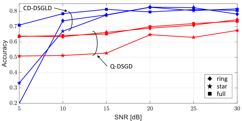
(a)

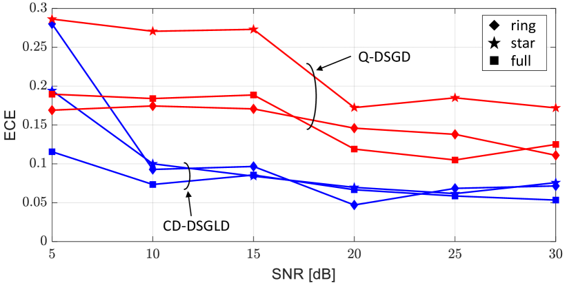
(b)

Fig. 2: Accuracy (a) and ECE (b) for the proposed CD-DSGLD scheme and for the conventional Q-DSGD as a function of the SNR for full, ring, and star topologies.

This section presents experiments used to evaluate the performance of CD-SGLD against the conventional digital implementation of DSGD, Q-DSGD, reviewed in the previous section.

5.1 Simulation Setting

We consider a cooperative sensing use case, where $N=5$ vehicles collaborate to detect and classify 6 different road users/objects from point cloud data gathered by on-board lidar as in [4]. To infer the road object categories, vehicles rely on a PointNet DNN implemented as in [4], with $m=40\text{,}855$ parameters and $40$ trainable layers. The agents hold a training dataset composed by $40$ examples for each one of the 6 classes, and the performances are evaluated over a separated validation dataset comprised by $2\text{,}400$ examples evenly partitioned across the 6 classes. We consider three different connectivity patterns for assessing the performances: (i) a fully connected topology, (ii) a star topology and (iii) a ring topology.

5.2 Implementation

For both CD-DSGLD and Q-DSGD, we set the learning rate to $\eta=10^{-4}$, and the total number of iterations to $s=15\text{,}000$. For CD-SGLD, we follow the standard approach of discarding the first samples produced during the “burn-in” period [14]. The burn-in period is is set to $14,900$ iterations. Furthermore, we adopt a standard Gaussian $\mathcal{N}(0,\mathbf{I}_{m})$ as the prior $p(\boldsymbol{\theta})$. For both methods, we set $w=2/\lambda_{1}(\mathbf{L}+\lambda_{N-1}(\mathbf{L}))$, where $\mathbf{L}$ is the Laplacian matrix of the graph $\mathcal{G}=(\mathcal{N},\mathcal{E})$, while $\lambda_{\ell}(\mathbf{L})$ denotes the $\ell$-th eigenvalue of $\mathbf{L}$ [23].

5.3 Performance Metrics

As performance metrics, we consider the standard measure of test accuracy and the Expected Calibration Error (ECE), with the latter quantifying the ability of the model to provide reliable uncertainty measures [24]. The ECE is evaluated based on the confidence level produced by the model as the maximum probability assigned by the last, softmax, layer to the possible outputs. The ECE measures how well the confidence levels reflect the true accuracy of the decision corresponding to the maximum probability, and it is computed as follows. At first, the test set is divided into a set of $T$ bins $\{B_{t}\}_{t=1}^{T}$ and for each bin $B_{t}$ the average accuracy $\text{acc}(B_{t})$ and confidence $\text{conf}(B_{t})$ are computed. Then, the ECE is computed by taking into account all accuracy/confidence values for all bins as [24]

$$\text{ECE}=\sum_{t=1}^{T}\dfrac{|B_{t}|}{n}|\text{acc}(B_{t})-\text{conf}(B_{t})|\,,$$ (12)

where $|B_{t}|$ and $n$ denote the number of examples in the $t$-th bin and the overall number of examples in the validation set, respectively.

5.4 Results

Fig. 2 reports the test accuracy and the ECE of CD-DSGLD and Q-DSGD as a function of the SNR, defined as $\mathrm{SNR}=P/N_{0}$. The main conclusion from the figure is that Bayesian FL via CD-DSGLD can significantly enhance the calibration as compared to frequentist FL implemented via Q-DSGD, as long as the SNR is sufficiently large. The advantages of CD-DSLGD in terms of calibration come at the cost of a lower accuracy at low values of the SNR if the connectivity of the network is reduced. In this case, the excessive channel noise does not match well the requirement of DSGLD, causing a performance loss for CD-SGLD. However, for sufficiently large SNR, or for a well-connected network at all SNRs, CD-DSGLD outperforms Q-DSGD both in terms of accuracy and calibration.

6 Conclusions

This paper has proposed a novel channel-driven Bayesian FL strategy for decentralized, or D2D networks where over-the-air computing is exploited to aggregate the samples during the wireless propagation. The experimental results considered a challenging cooperative sensing task for automotive applications, and confirmed the superior performance of the proposed method in providing more accurate uncertainty quantification as compared to a frequentist FL method based on standard digital transmission of quantized model parameters. Future works will target the integration of more complex channel models.

References

- [1] H. B. McMahan, E. Moore, D. Ramage et al., “Communication-efficient learning of deep networks from decentralized data,” arXiv e-prints, 2016.
- [2] T. Li, A. K. Sahu, A. Talwalkar, and V. Smith, “Federated learning: Challenges, methods, and future directions,” IEEE Signal Processing Magazine, vol. 37, no. 3, pp. 50–60, 2020.
- [3] S. Savazzi, M. Nicoli, M. Bennis et al., “Opportunities of federated learning in connected, cooperative, and automated industrial systems,” IEEE Communications Magazine, vol. 59, no. 2, pp. 16–21, 2021.
- [4] L. Barbieri, S. Savazzi, M. Brambilla, and M. Nicoli, “Decentralized federated learning for extended sensing in 6g connected vehicles,” Vehicular Communications, p. 100396, 2021.
- [5] O. Simeone, Machine Learning for Engineers. Cambridge University Press, 2022.
- [6] R. Kassab and O. Simeone, “Federated generalized bayesian learning via distributed stein variational gradient descent,” IEEE Transactions on Signal Processing, vol. 70, pp. 2180–2192, 2022.
- [7] J. Gong, O. Simeone, and J. Kang, “Compressed particle-based federated bayesian learning and unlearning,” arXiv e-prints, 2022.
- [8] D. M. Blei, A. Kucukelbir, and J. D. McAuliffe, “Variational inference: A review for statisticians,” Journal of the American Statistical Association, vol. 112, no. 518, pp. 859–877, 2017.
- [9] E. Angelino, M. J. Johnson, and R. P. Adams, “Patterns of Scalable Bayesian Inference,” arXiv e-prints, Feb. 2016.
- [10] M. Ashman, T. D. Bui, C. V. Nguyen et al., “Partitioned variational inference: A framework for probabilistic federated learning,” CoRR, vol. abs/2202.12275, 2022.
- [11] S. Ahn, B. Shahbaba, and M. Welling, “Distributed stochastic gradient mcmc,” in Proceedings of the 31st International Conference on Machine Learning, ser. Proceedings of Machine Learning Research, E. P. Xing and T. Jebara, Eds. Bejing, China: PMLR, 22–24 Jun 2014, pp. 1044–1052.
- [12] M. Garbazbalaban, X. Gao, Y. Hu, and L. Zhu, “Decentralized Stochastic Gradient Langevin Dynamics and Hamiltonian Monte Carlo,” Journal of Machine Learning Research, vol. 22, no. 239, pp. 1–69, 2021.
- [13] M. Welling and Y. W. Teh, “Bayesian learning via stochastic gradient langevin dynamics,” in Proceedings of the 28th International Conference on Machine Learning, ser. ICML’11. Omnipress, 2011, p. 681–688.
- [14] D. Liu and O. Simeone, “Wireless Federated Langevin Monte Carlo: Repurposing Channel Noise for Bayesian Sampling and Privacy,” arXiv e-prints, Aug. 2021.
- [15] X. Cao, G. Zhu, J. Xu et al., “Optimized power control design for over-the-air federated edge learning,” IEEE Journal on Selected Areas in Communications, vol. 40, no. 1, pp. 342–358, 2022.
- [16] K. Yang, T. Jiang, Y. Shi, and Z. Ding, “Federated learning via over-the-air computation,” IEEE Transactions on Wireless Communications, vol. 19, no. 3, pp. 2022–2035, 2020.
- [17] C. Xu, S. Liu, Z. Yang et al., “Learning rate optimization for federated learning exploiting over-the-air computation,” IEEE Journal on Selected Areas in Communications, vol. 39, no. 12, pp. 3742–3756, 2021.
- [18] R. Xin, S. Kar, and U. A. Khan, “An introduction to decentralized stochastic optimization with gradient tracking,” arXiv e-prints, Jul. 2019.
- [19] W. Shin, M. Vaezi, B. Lee et al., “Non-orthogonal multiple access in multi-cell networks: Theory, performance, and practical challenges,” IEEE Communications Magazine, vol. 55, no. 10, pp. 176–183, 2017.
- [20] D. Alistarh, D. Grubic, J. Li et al., “QSGD: Communication-Efficient SGD via Gradient Quantization and Encoding,” arXiv e-prints, Oct. 2016.
- [21] S. Shi, X. Chu, K. C. Cheung, and S. See, “Understanding Top-k Sparsification in Distributed Deep Learning,” arXiv e-prints, Nov. 2019.
- [22] F. Sattler, S. Wiedemann, K. Müller, and W. Samek, “Sparse binary compression: Towards distributed deep learning with minimal communication,” in 2019 International Joint Conference on Neural Networks (IJCNN), 2019, pp. 1–8.
- [23] H. Xing, O. Simeone, and S. Bi, “Federated learning over wireless device-to-device networks: Algorithms and convergence analysis,” IEEE Journal on Selected Areas in Communications, vol. 39, no. 12, pp. 3723–3741, 2021.
- [24] C. Guo, G. Pleiss, Y. Sun, and K. Q. Weinberger, “On Calibration of Modern Neural Networks,” arXiv e-prints, Jun. 2017.