Resolving the Vicinity of Supermassive Black Holes with Gravitational Microlensing

Abstract

In the near future, wide field surveys will discover 1000’s of new strongly lensed quasars, and these will be monitored with unprecedented cadence by the Legacy Survey of Space and Time (LSST). Many of these will undergo caustic-crossing microlensing events over the 10-year LSST survey, in which a sharp caustic feature from a stellar body in the lensing galaxy crosses the inner accretion disk. Caustic-crossing events offer the unique opportunity to probe the vicinity of the central supermassive black hole for 100s of quasars with multi-platform follow-up triggered by LSST monitoring. To prepare for these observations, we have developed detailed simulations of caustic-crossing light curves. These employ a realistic analytic model of the inner accretion disk that reveals the strong surface brightness asymmetries introduced when fully accounting for both special- and general-relativistic effects. We demonstrate that an inflection in the caustic-crossing light curve due to the innermost stable circular orbit (ISCO) can be detected in reasonable follow-up observations and can be analyzed to constrain ISCO size. We also demonstrate that a convolutional neural network can be trained to predict ISCO size more reliably than traditional approaches and can also recover source orientation with high accuracy.

1 Introduction

Active Galactic Nuclei (AGN) play an integral role in the evolution of galaxies and are important probes of the distant universe. It is generally accepted that they are powered by the conversion of gravitational potential energy into thermal continuum radiation through the accretion of material onto a central Super Massive Black Hole (SMBH) (Salpeter, 1964; Zel’dovich, 1964). This radiation is then reprocessed through a variety of mechanisms into emission that spans the electromagnetic spectrum (see Padovani et al., 2017, for a review). Especially luminous AGNs with unobscured accretion disks are known as quasars and are visible even at extreme cosmological distances (e.g. Mortlock et al., 2011; Bañados et al., 2018). At their great distances, the $\sim$light day accretion disk has an angular scale of nano- to micro-arcseconds, and cannot be spatially resolved by direct imaging. The region in the vicinity and under the direct influence of the SMBH is two orders of magnitude smaller than the optical disk, and hence is likely to remain inaccessible to direct observational methods.

There are currently three non-conventional methods for probing the vicinity of accreting SMBHs–two of which have been successfully realized. The Event Horizon Telescope has recently yielded our first image of the vicinity of an accreting SMBH (Event Horizon Telescope Collaboration et al., 2019), and Very Long Baseline Interferometry on GRAVITY is sensitive to relativistic effects of our Galaxy’s SMBH on closely orbiting stars (Gravity Collaboration et al., 2017). Continuum reverberation mapping, especially combined with Doppler boosting of the iron K$\alpha$ emission line, has been used to probe kinematics and geometry within several gravitational radii of SMBHs (see Cackett et al., 2021, for a review). The third approach, which is yet to be fully exploited, offers the potential to scan the accretion disk of strongly-lensed quasars on the scale of the gravitational radius using the natural magnification boost provided by gravitational microlensing.

Gravitational lensing of a quasar due to a sufficiently massive object (typically a galaxy) along the line of sight can result in multiple observable images of the quasar and its host galaxy. Individual images of such strongly lensed quasars frequently exhibit microlensing: fluctuations in magnification caused by inhomogeneities in the mass distribution of the lensing galaxy due to compact, stellar-mass objects (see Wambsganss, 2006, for review). These inhomogeneities create a complex magnification structure in the source plane, referred to as a caustic network, which can exhibit strong variations on the micro to nano-arcsecond scales. This results in differential magnification of quasar central engines on a ranges of scales, and this differential microlensing is time-varying due to the relative transverse motion of the lens and source.

Analysis of microlensing fluctuations has lead to constraints on the sizes and geometries of quasar emission regions, from the accretion disk (e.g. Pooley et al., 2007; Morgan et al., 2010; Blackburne et al., 2011, 2014, 2015; Jiménez-Vicente et al., 2012, 2014; Muñoz et al., 2016; Morgan et al., 2018) to the Broad Emission Line Region (BELR) (e.g. Schneider & Wambsganss, 1990; Hutsemekers et al., 1994; Lewis & Belle, 1998; Abajas et al., 2002; Sluse et al., 2007; Sluse et al., 2011; O’Dowd et al., 2011, 2015; Paic et al., 2021; Williams et al., 2021). Accretion disk studies have typically placed constraints on the size and/or temperature gradient of the accretion disk. However, microlensing also has the potential to resolve the vicinity of the SMBH down to $R_{\rm g}$, the gravitational radius. Individual caustic folds and cusps can produce magnification changes up to $\mathcal{O}(10^{3})$ over their nanoarcsecond-scale gradients for an appropriately small source, such as an accretion disk seen in ultra-violet or X-ray wavelengths. These events are rare ($\approx 1$ per decade, per system Mosquera & Kochanek, 2011), unfold quickly within a few weeks or months (e.g. Neira et al., 2020), and there is only scarce evidence for their presence in existing data. Q2237+0305 –the Einstein Cross– is the most likely system for displaying this behaviour due to its exceptionally large relative transverse velocity that leads to an increased rate of caustic crossings. In this system, Mediavilla et al. (2015) identified the possible signature of the “black hole shadow” within the Innermost Stable Circular Orbit (ISCO). However no event has yet been observed with sufficient cadence, depth, and wavelength coverage to place strong constraints on this or other properties of the curved spacetime around the SMBH.

Microlensing of quasars can be analyzed using various degrees of complexity in accretion disk models. A common choice is the physically motivated thin disk model (Shakura & Sunyaev, 1973) that has an exponential brightness profile. Outside the high-magnification regime of a caustic-crossing event, microlensing is relatively insensitive to the detailed temperature profile, depending instead on the overall size of the disk (the half-light radius) (Mortonson et al., 2005; Vernardos & Tsagkatakis, 2019). As such, many studies use simplified profile shapes such as Gaussians in their simulation, with an appropriate scaling of half-light-radius to observed wavelength to approximate a thin disk profile (Grieger et al., 1988; Agol & Krolik, 1999; Wyithe et al., 2002; Kochanek, 2004; Bate et al., 2008; Jiménez-Vicente et al., 2014; Bate et al., 2018; Tomozeiu et al., 2016). Although this is sufficient for long-term microlensing studies, the detailed structure of the disk near the ISCO is expected to be magnified and imprint itself on the light curve during a high magnification event. Abolmasov & Shakura (2012) use a simple thin-disk model as well as a relativistic one obtained numerically to explain high magnification events observed in Q2237+0305. They consider relativistic effects only through a Doppler boost manifested by a frequency shift calculated along the photon geodesics. Mediavilla et al. (2015) use both a classic as well as a relativistic thin disk model in order to fit data for three high magnification event candidates observed in Q2237+0305. Their relativistic model calculates the effect of relativistic beaming alongside Doppler shift and gravitational redshift, which effectively improves their fit to observed data. Tomozeiu et al. (2016) adopt a simpler approach using a crescent shaped accretion disk model to approximate a simulation of a caustic-crossing event in M87. Their model is designed to fit simulated data created from the convolution of a general relativistic magneto-hydrodynamic simulation in (Dexter et al., 2010) and a clean caustic fold. None of these studies have included lensing by the SMBH calculated via geodesic tracing of light rays, which can have a significant impact on the innermost regions of the accretion disk.

In the next few years, high magnification events are expected to turn from a curiosity into routinely encountered phenomena. This is largely due to the Legacy Survey in Space and Time (LSST) to be carried out at the Vera C. Rubin Observatory. In concert with Euclid, LSST will discover several thousand strongly-lensed quasars (Oguri & Marshall, 2010) and monitor them with a cadence of a few days. Over its 10-year survey, approximately 5% of these lensed quasars are expected to undergo caustic-crossing events (Mosquera & Kochanek, 2011), resulting in upwards of 300 events per year (Neira et al., 2020). If an impending caustic-crossing event could be identified with LSST monitoring, multi-platform observations spanning the event peak would yield unprecedented information about the structure of the quasar inner disk and SMBH vicinity.

In order to design appropriate caustic-crossing followup, detailed and realistic simulations of these events are essential. In this paper we describe simulations of caustic-crossing light curves that employ a realistic analytic model of the inner accretion disk and a proper accounting of all relativistic effects. We then apply both traditional and machine-learning analysis methods to the extraction of the inner disk and SMBH properties, and we study the observational requirements for the successful followup of caustic-crossing events. In Section 2 we describe the accretion disk and microlensing models that we use and present the resulting features of our simulated light curves. We analyze these mock observations using two different approaches: 1) measuring the size of the ISCO from a spline fit’s derivative and a wavelet transform of the light curve, presented in Section 3, and 2) using supervised machine learning to access the full non-linear parameter space of the problem to predict the size of the ISCO, the mass of the SMBH and inclination of the disk, presented in Section 3.3. Our results are presented in Section 4, where we compare the recovered ISCO size of the analytic method with the predicted values of the convolutional neural network. In Section 5, we present our outlook on these methods of analysis and discuss the implications/requirements for future high magnification event observations. Within this work, we assume a flat $\lambda$CDM cosmology with Hubble Constant 70 km/s/Mpc and $\Omega_{0}$ = 0.3.

2 Simulated dataset

Light curves of accretion disk caustic-crossing events are simulated by taking the convolution of a model surface brightness map of the accretion disk (Section 2.1) along with a simulated microlensing magnification map (Section 2.2). The angular diameter distance is used to explicitly calculate distances in the source plane. Photometric noise is added and the cadence of observations is assumed according to a reasonable intensive follow-up observation of the caustic-crossing event (Section 2.3), with fluxes calculated from luminosity distances at the source plane. Specific characteristics of the disk model that we eventually want to extract, like the size of the ISCO, are visibly encoded in the features of the simulated light curves (e.g. see Fig. 4).

2.1 Accretion disk model

2.1.1 Relativistic extensions to the thin disk model

Our starting point is the standard thin disk model (Shakura & Sunyaev, 1973) to which we add the following relativistic effects: Doppler shifting of the continuum, Doppler beaming, and local gravitational lensing by the SMBH. It is important to distinguish strong lensing and microlensing that require a lens at a cosmological distance away from the source and this lensing effect that takes place in the local strongly curved spacetime around the SMBH even in non-multiply imaged quasars. The temperature profile of a thin disk is given by:

$$T(r)=\left[\frac{GM_{\rm BH}\dot{M}_{\rm BH}}{8\pi\sigma r^{3}}\left(1-\sqrt{\frac{R_{\rm in}}{r}}\right)\right]^{1/4}\,,$$ (1)

where $M_{\rm BH}$ is the SMBH mass, $\sigma$ is the Stefan-Boltzmann constant, and $R_{\rm in}$ is the inner boundary of the disk that we assume to be the ISCO, i.e. $R_{\rm in}=\alpha GM_{\rm BH}/c^{2}$, where $\alpha$ depends on SMBH spin relative to the accretion disk ($\alpha=$ 6, 2, or 9 for non-rotating, maximally prograde, and maximally retrograde respectively). The accretion rate, $\dot{M}_{\rm BH}$, can be expressed in terms of the Eddington ratio $R_{\rm Edd}=L/L_{\rm Edd}$, where: $L_{\rm Edd}=GM_{\rm BH}\dot{M}_{\rm BH}/2R_{\rm in}$. Using equation (1) and matching the given temperature to black body emission, we can obtain the flux of the disk as a function of radius and (rest) wavelength. We assume that the region interior to the ISCO does not emit any photons that reach the observer. By taking the inclination angle $\theta_{\rm inc}$ into account ($0\degree$ is face on), we project the accretion disk onto the source plane to obtain the two-dimensional projected surface brightness map of a thin-disk. Before extending this basic model with relativistic effects, we account for Doppler shifting due to the disk’s rotation. This is done by assuming a Keplerian velocity profile that is similarly projected on the source plane using the inclination angle.

The closer we get to the SMBH, i.e. $R_{\rm in}$ or the ISCO, the greater the asymmetry becomes between the approaching and receding sides. First we consider the Doppler shift and Doppler beaming due to the line-of-sight velocity of the accretion material. Due to Doppler shifting, we calculate the intensity of black body radiation that gets shifted into the desired observed wavelength. This shift is calculated explicitly, and can either result in an increase or decrease in the intensity. Doppler beaming then amplifies (diminishes) emission from the approaching (receding) side of the accretion disk.

The asymmetries induced by Doppler shift and beaming are further enhanced by local gravitational lensing by the SMBH. We simulate this using the general relativistic ray tracing code GYOTO (Vincent et al., 2011) and find that it primarily impacts the inner regions of the disk. Our Doppler-shifted and beamed surface brightness maps are lensed through an appropriate Kerr metric (Kerr, 1963) calculated using the local SMBH mass and spin parameters to yield the final projected surface brightness distribution prior to any microlensing. Figure 1 shows incremental contributions to the asymmetry due to relativistic effects as they are added.

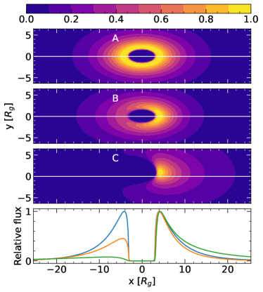
Figure 1: Normalized projected relative surface brightness profiles of an accretion disk at an inclination angle of $\theta_{\rm inc}=60\degree$. Panel A: Prior to any relativistic effects the thin disk appears symmetric. B: Once relativistic beaming and Doppler shifts are included, the approaching side is $\sim 2$ times brighter than the receding one. C: Tracing the photon geodesics in a strongly curved Kerr spacetime due to the SMBH (SMBH lensing), the brightness ratio between the two sides of the disk is $\sim 10$. The bottom panel shows the relative brightness of along a horizontal line passing through the disk’s central axis for each of the profiles in the A, B, C panels (blue, orange, and green respectively).

2.1.2 Resulting surface brightness maps

We illustrate the result of including each of the relativistic effects introduced above in Fig. 1. Prior to the introduction of relativistic effects, the disk appears symmetric around the optical axis. Introducing Doppler shift and relativistic beaming results in the brightening (dimming) for line-of-sight velocities towards (away from) the observer. This leads to a factor of $\sim 2$ asymmetry in surface brightness between the approaching and receding sides of the inner disk.

The region surrounding the ISCO emits accretion disk photons that have travelled along curved paths around the SMBH. These photons receive a Doppler boost determined by the velocity component of the accretion disk at the point of emission. This boosting velocity will always be in the same direction (approaching/receding/transverse) as the region of the disk projected on the plane of the sky from which that photon appears to emerge. The boost is relative to the alignment of the accreted material’s velocity and the geodesic which reaches the observer at the point of emission. The result is significant enhancement of the surface brightness asymmetry from relativistic beaming—a factor of $\sim 10$ for the case of $\theta_{\text{inc}}=60\degree$ in Fig. 1.

This asymmetry in brightness between the approaching and receding sides of the disk depends heavily on the inclination angle. As shown in Fig. 2, the asymmetry increases sharply as we approach an edge-on orientation. Because edge-on disks are thought to be obscured by dusty tori surrounding them, we do not expect such extreme inclinations in observed quasars. Note that this change in inclination results in elongated disks that have different apparent sizes along different directions, which can affect the inferred disk size depending on the impact angle with respect to a caustic (see Section 2.3). However, the apparent width of the ISCO is not subject to the same elongation/contraction.

For ISCOs that are elongated due to large inclination angles, lensing by the SMBH causes the far side of the ISCO to become rounded, so that only the near side of the ISCO appears significantly contracted, as shown in Fig. 3 where the near side is on bottom, and the far side is on top. Simulations suggest that the ISCO size along a given direction can vary by a factor of 0.7, as shown in Fig. 2.

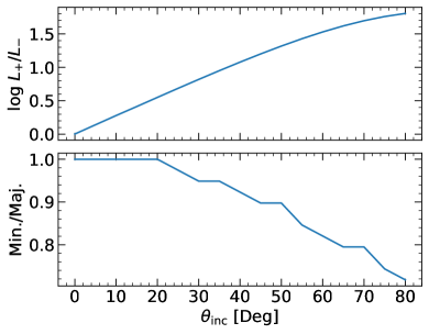
Figure 2: Effect of the inclination angle $\theta_{\rm inc}$ on the accretion disk asymmetry found through GYOTO simulations. Top: Brightness ratio between points at $1R_{\rm g}$ on the approaching/receding sides of the disk, marked by the crosses in Fig.  3, as a function of $\theta_{\rm inc}$. Bottom: The projected ISCO compression (Minor axis / Major axis) as a function of $\theta_{\rm inc}$. Values represent the ratio of the minor and major axes of the ISCO.

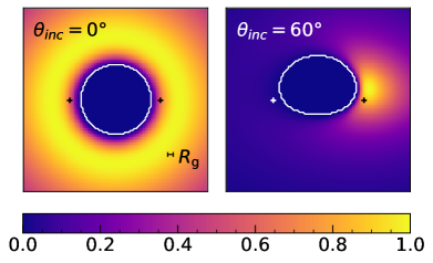
Figure 3: Central region of the accretion disk for $\theta_{inc}=0\degree~{}\text{and}~{}60\degree$. The approaching side of the accretion disk is on the right. Crosses mark the locations used to calculate the ratio shown in Figure 2. The horizontal bar overlaid on the image indicates $1R_{\rm g}$. The center white contour is placed at the ISCO for clarity. The colorbar denotes the relative flux from each region of the accretion disk.

2.2 Lens Model

The caustic network produced by an ensemble of stellar-mass compact objects depends on the local values of the convergence and shear within the lensing galaxy at the positions of the macroscopically observed quasar multiple images. This can vary from isolated diamond-shaped caustics to dense networks of overlapping and nested ones (see the GERLUMPH database for examples). Despite this, the basic property of a caustic, i.e. being the locus where magnification of a point source nominally diverges, and even its analytical description remain unchanged (Fluke & Webster, 1999). This means that if a source is smaller than the distance between two consecutive caustics then all caustic crossing events can be treated as isolated. Here we use such an isolated caustic to produce our mock light curves, expecting our results to be applicable also in cases of more complicated caustic structures as long as the source is small enough.

We produce a high-resolution zoomed-in version of a magnification map around an isolated caustic of a GERLUMPH map using the GPU-D code (Thompson et al., 2010). The size of the map is 1.0 Einstein radius, $R_{\rm E}$, and the resolution $10^{4}$ pixels per side. The stellar and smooth convergence components have been set to 0.328 and 0.082 respectively, and the shear to 0.38. To produce caustic-crossing light curves, we convolve our accretion disk surface brightness profile with the magnification map and draw different trajectories across it. Such example trajectories are shown in Fig. 4 and a specific example of a simulated light curve is shown in Fig. 5.

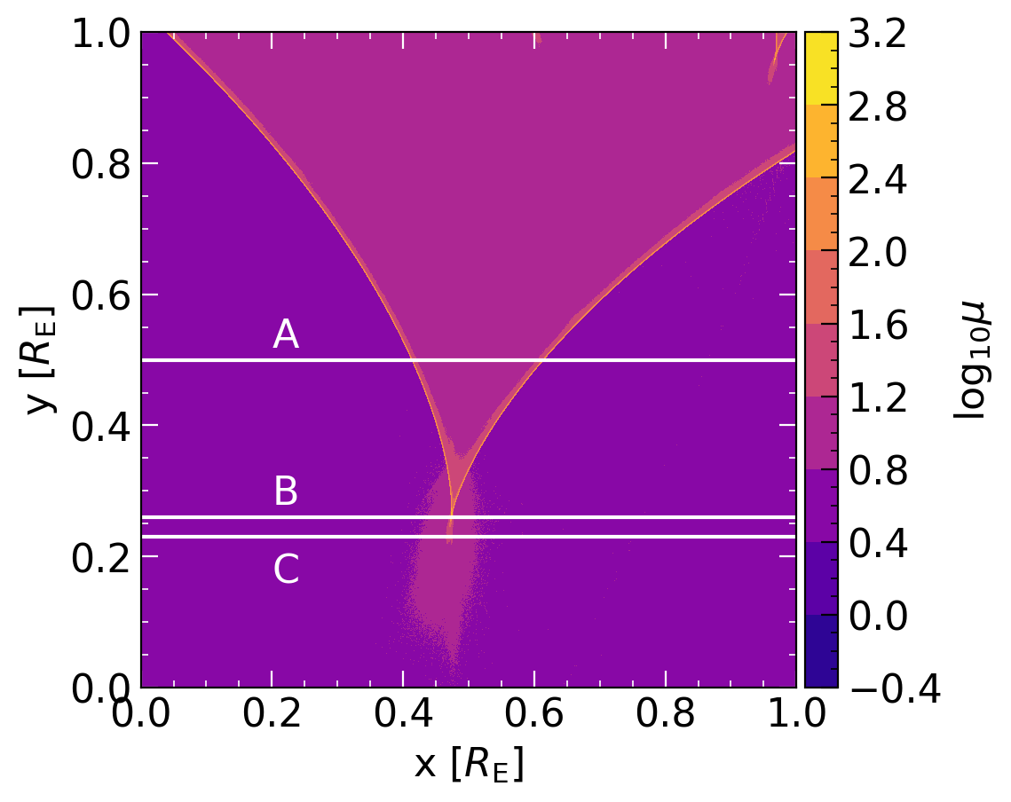
Figure 4: Magnification map zoomed-in around an isolated caustic used in simulating caustic-crossing events. Example light curve tracks are shown for a fold (A) and cusp crossing (B), and for a near miss of the cusp (C). The colorbar denotes the logarithm of the magnification.

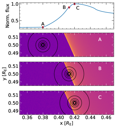
Figure 5: Top: Sample light curve. The labelled points correspond to the panels below, which show the accretion disk brightness profile for a SMBH viewed face on. The accretion disk is represented by 5 equally spaced black contours placed at 0.2, 0.4, 0.6, 0.8, and 1.0 of the peak flux. Position A represents the start of the observed rise in brightness, B the start of the ISCO crossing, and C the peak brightness.

2.3 Simulating light curves

The free parameters of our accretion disk model are: the SMBH mass and spin, the mass accretion rate (Eddington ratio), and the inclination angle. We note that there are some degeneracies present, e.g. for a given ISCO the SMBH mass and spin are degenerate, which we will need to take into account in interpreting our measurements (see Section 3). The lensing parameters consist of the impact angle and the magnification map parameters, although the latter are less important due to the universal behaviour of an isolated caustic crossing event. There is another important degeneracy introduced here: It is not the absolute but the relative size of the accretion disk with respect to the $R_{\rm E}$ of the microlens(es) that determines the imprints of its detailed structure on the resulting light curves during a caustic crossing. We detail our choices of all parameters in this section and note that the parameter space explored is not intended to be exhaustive, but rather to allow us to explore the performance of measuring these properties for a wide range of possible parameters.

For the SMBH mass we assume the range $10^{7}<$M${}_{\rm BH}<10^{9.7}$, which approximately spans the SMBH mass range for quasars with dynamically measured masses (McConnell & Ma, 2013). Larger masses result in accretion disks much larger than $R_{\rm E}$, and the convolution smears out the caustic to the point where the ISCO crossing is absent from the light curves. In a similar way, lower masses correspond to extremely small ISCO sizes that require unrealistically high-cadence observations to resolve (see below). In addition to the mass, the size of the ISCO depends on the SMBH spin and is expected to be between $2GM/c^{2}$ and $9GM/c^{2}$, with limiting cases for a maximally-rotating Kerr black hole with prograde and retrograde accretion respectively. In this work, we do not consider this degeneracy but rather explore the case of a non-rotating black hole, acknowledging that any ISCO measurement implies a $\sim 1$dex range of masses depending on spin. We assume an accretion rate such to yield an Eddington ratio of $L/L_{Edd}=0.15$, chosen as fairly typical of a moderately powerful quasar at $z\sim 1$ Kelly et al. (2010). The thin disk model is not expected to apply for significantly higher Eddington ratios, where more efficient accretion modes are needed. We set $z_{\text{lens}}=0.5$ and explore $1<z_{\text{source}}<3$ for all of our simulations, corresponding to the peak of lens redshift and spanning the peak of source redshift expected for lensed quasar systems to be discovered by LSST (Oguri & Marshall, 2010). Finally, we explore lines of sight with $\theta_{\text{inc}}<75\degree$, assuming that larger inclinations (more edge-on disks) suffer obscuration by the dusty torus (Antonucci, 1993).

The most important lensing parameters are the Einstein radius and the impact angle of the accretion disk trajectory on the source plane with respect to the caustic. The Einstein radius of the microlens ($R_{\rm E}$) depends on the mass of the microlens, the lens and source redshifts, and cosmology through the angular diameter distances to the lens, source, and between them. For microlensing, Mosquera & Kochanek (2011) describes how the relative size scale of the disk (defined therein as $R_{\rm S}$) with respect to $R_{\rm E}$ is what determines fluctuations. Within their sample of lensed quasars, this ratio was determined to be $0.001<R_{\rm S}/R_{\rm E}<0.25$. This closely matches the ranges explored in this study, with $4.1\times 10^{14}\rm m<R_{\rm E}<5.3\times 10^{14}$ m, and our $8.8\times 10^{10}\rm m<R_{\rm S}<4.4\times 10^{13}\rm m$, which correspond to source redshifts between 1 and 3, SMBH masses quoted above, and a $1\rm M_{\odot}$ microlens mass.

As shown in Figures 1 and 2, the inclination angle plays an important role in the shape of the disk’s brightness profile, causing it to appear elongated along an axis. It turns out that the angle of this axis, $\phi$, with respect to the direction of motion across a caustic plays an important role too. We define this impact angle of $\phi=0\degree$ corresponds to neither the brightened side nor the dimmed side crossing the caustic first but instead a symmetric crossing which is identical to the $\phi=180\degree$ case. An angle of $\phi=\pm 90\degree$ corresponds to the receding/approaching side of the accretion disk crossing the caustic first.

In this work we simulate optical followup with an 8-meter class telescope. We calculate our signal-to-noise ratio using the Gemini South Integration Time Calculator for GMOS imaging, assuming 1 hour exposures in the targeted optical bands and with best observing conditions. The cadence of the observations is set in terms of the Einstein radius because the actual transverse velocity of the disk across the magnification map can vary greatly (see Neira et al., 2020, for a presentation of such an effective velocity model). We simulate evenly spaced observations such that each time interval between observations has a length of $10^{-4}R_{\rm E}$. For example, if we were to assume an effective velocity of 500 km/s, this would lead to a cadence of approximately one observation per day.

2.4 Light curve features

Figure 6 shows a selection of simulated caustic-crossing light curves spanning the range of explored parameters at $\lambda_{\rm obs}=600\text{nm}$, in this case without photometric errors. An overall feature of the light curves is a rise in the integrated flux as the caustic curve sweeps across the disk, peaking roughly when it crosses the ISCO region before dropping away. The accretion disk size determines the steepness of the magnification change. The most interesting part of these light curves is the detailed structure of the signal that appears at the peak. For a symmetric disk, i.e. in the absence of relativistic effects, the ISCO crossing commonly results in a double-peak feature superimposed on the light curve peak. The asymmetry in surface brightness produced by Doppler shifting, beaming, and lensing suppresses one of these peaks and enhances the other, resulting in an inflection rather than a double peak. This is evident when comparing cases where neither the enhanced/suppressed side crosses the caustic first ($\phi=0\degree$ or $180\degree$), or exactly the face on case ($\theta_{\text{inc}}=0\degree$) to the case where this enhanced/suppressed side crosses first, as in the bottom two panels of Fig. 6. Asymmetry increases with increasing $\theta_{\mathrm{inc}}$ and as the impact angle changes towards the enhanced/suppressed side crossing the caustic first.

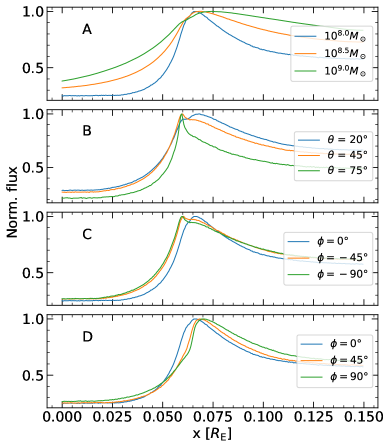
Figure 6: Effect of the various parameters on light curves (normalized units). A) Light curves widen with black hole mass ($M_{BH}$) but the inflection due to the ISCO crossing is still there, for $\theta_{\text{inc}}=45\degree,\phi=0\degree$. B) Light curves for different $\theta_{\mathrm{inc}}$ for a disk with its approaching side crossing first. C) Effect of impact angle $\phi$ such that the approaching side crosses first. D) Effect of $\phi$ such that the receding side crosses first. These last two panels show that the double-peak feature is almost entirely absent when the receding side crosses first.

Multi-wavelength observations can add significant information and potentially break a number of degeneracies. Fig. 7 demonstrates a single caustic-crossing event in various optical bands. The width of the caustic-crossing event in the different filters depends on the size of the accretion disk, which for a non-relativistic disk would be given by equation (1). Disk size increases with observed wavelength, and so the ratio of event widths between different bands gives us a measure of the accretion disk temperature gradient (e.g. Wambsganss & Paczynski, 1991; Anguita et al., 2008; Bate et al., 2018, etc). Figure 8 shows the same multi-wavelength light curves including simulated noise, assuming observations by an 8m-class telescope with 1 hour exposure times and an effective velocity that yields a spatial resolution of $\approx 10^{-4}R_{\mathrm{E}}$. We highlight how with 1 hour exposures, the ISCO crossing can even be seen in some shorter wavelength bands at high ($z_{\rm source}\sim 3$) redshift.

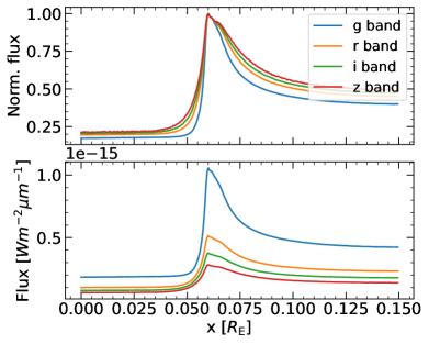
Figure 7: Mock light curve in different bands for a fold caustic crossing event with $M_{\rm BH}=10^{8}M_{\odot}$. Top: Normalized light curves show the general widening of the crossing event but the same ISCO size. Bottom: shorter optical bands are significantly brighter and more magnified during the event.

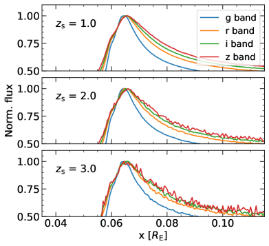
Figure 8: Light curves with photometric errors for disks at three redshifts. Each band is normalized separately to its own maximum value to emphasise that the ISCO crossing feature remains the same but the errors due to lower signal-to-noise ratios may hide it. Each simulation depicted uses a $10^{8}M_{\odot}$ black hole approaching the caustic beamed side first at $\theta_{\text{inc}}=45\degree$. At $z_{\text{source}}$ = 1.0, photometric noise is low in all bands. For $z_{\text{source}}$ = 2.0, the g and r bands appear reasonably smooth, while the signal-to-noise ratio in the i and z bands decreases. At $z_{\text{source}}$ = 3.0, the effect of higher photometric noise (less photons) is seen in all bands. The ISCO feature itself becomes less and less apparent with higher redshift.

3 Light curve analysis techniques

The accretion disk/SMBH properties with the most impact on the data are the size of the ISCO and the flux asymmetry (see Fig. 1). These manifest themselves in the double-peak feature of the light curves as the distance and height difference between the two peaks (see Fig. 6). The parts of the light curve that correspond to the ISCO entering and exiting a caustic are characterized by this drop in the flux between the two peaks, because there are no photons coming from within the ISCO. Apart from these somewhat intuitive features, the combination of all the parameters in our model ($M_{\rm BH}$, impact angle, inclination, etc) introduces non-linear features in the light curves that are less straightforward to identify and interpret.

We approach the problem first by measuring the lowest order effect, i.e. the size of the ISCO, using two methods to find the width of the ISCO-crossing feature: The second derivative of a spline fit and a wavelet transform. These are straightforward methods that are easy to implement and interpret. We acknowledge that this is accretion disk model dependent, as this would be sensitive to abrupt changes in the accretion disk profile, but emphasise that these variations should not occur in any smooth disk. Further experiments may be conducted in order to test how model dependent this method is. We then fit the data in the entire non-linear parameter space of the problem using a machine learning approach. Although evidently more powerful, this approach requires a more careful implementation and interpretation as opposed to the previous two methods.

3.1 Second derivative of spline fit

The dip in the light curve due to the ISCO-crossing event is bounded by a rapid change in its slope, which can be detected in the second derivative of a suitably smoothed light curve. This smoothing is performed by fitting a 3rd-order spline polynomial to the noisy mock light curves.

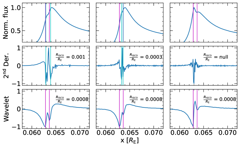
Figure 9: Measurements of the ISCO size for three example light curves. Top: Simulated light curves in normalized units. Center: Second derivative of the spline. The cyan vertical lines indicate the beginning and end of the ISCO crossing (also shown in the top row). Bottom: Wavelet detail coefficient amplitudes found through the wavelet transform. The magenta vertical lines indicate the beginning and end of the ISCO crossing (also shown in the top row). The explicitly calculated major axis in this case has $\frac{R_{\rm ISCO}}{R_{\rm E}}=0.00096$. We find good agreement for the 2^nd derivative method in the first case, and consistently decent agreement with the wavelet method in all cases.

Figure 9 shows the second derivative of the spline fit to the simulated data of three caustic-crossing events. The ISCO crossing manifests as a characteristic double-dip feature in the second derivative, with the minima corresponding to the entry and exit of the ISCO across the caustic curve. The ISCO size corresponds to the separation between the major dips of the second derivative. The spline fit proceeds by requiring the detection of two distinct minima in the second derivative, separated by a threshold. If the result is inconclusive, e.g. the derivative is dominated by noise, the spline’s smoothing parameters such as the knot density and positions are automatically adjusted through Scipy ’s Univariate Spline smoothness parameter ($s$) until the desired minima conditions are fulfilled. If there are too many detections of minima, $s$ is decreased randomly by 1% - 10%, and the second derivative’s minima are calculated. If there are too few detections of minima, $s$ is increased randomly by 1% - 10%, and minima are calculated. This is repeated 100 times and if the fit is still inconclusive then a null result is reported.

3.2 Wavelet transform

The double-peak feature of the ISCO crossing is a short-range feature in the data, with its peaks lasting only a fraction of the light curve length. This would allow it to be detected as a high frequency signal in the data, e.g. after applying a Fourier transform or a wavelet transform. Because we primarily care for the location of the peaks, a wavelet transform is better suited versus a Fourier transform. We employ the Daubechies wavelet basis (Daubechies, 1988) to detect the peaks of the ISCO crossing. We start by using a low band-pass filter, which is defined in the orthonormal wavelet basis as the approximation of the signal up to the scale $2^{j}$ where j is the order of the wavelet. A high band-pass filter then contains the details lost in making this approximation at the scale $2^{j-1}$, and is therefore sensitive to sharp changes in the transformed object (in this case, our light curve) (see Mallat, 2008, Chap. 7 for further reading). We look at the wavelet coefficient amplitudes in the details lost for the loss of this abrupt feature as the ISCO crossing event starts and stops. If we lose this crossing detail explicitly on both sides of the crossing, i.e. we find these two peaks in the wavelet coefficients separated by a threshold, then we accept this as a detection. The difference in the positions of these two peaks are recorded as the length of the ISCO. The module PyWavelets (Lee et al., 2019) was used for this analysis.

Figure 9 shows that the ISCO crossing manifests as a characteristic double-dip feature in the detail of the wavelet transform with the minima corresponding to the entry and exit of the ISCO across the caustic curve and their separation to the size of the ISCO - exactly in the same way as for the spline method. The offset with respect to the results of the spline method is because the wavelet basis functions have a finite width (in data space), which shifts the location of the feature after convolution.

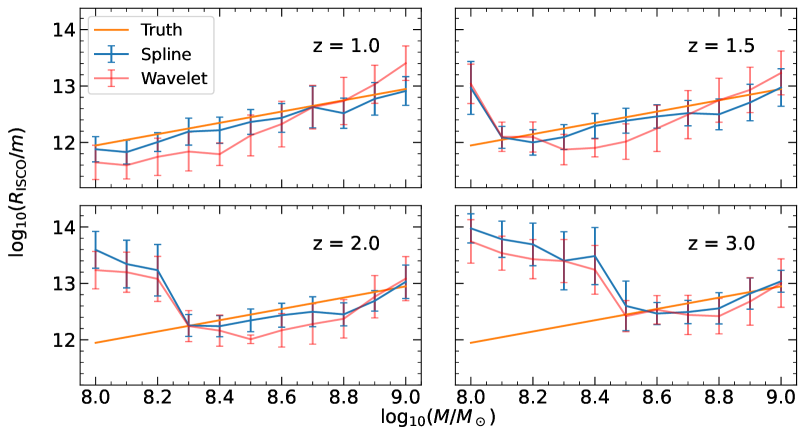
Figure 10: Measured ISCO width using the spline (blue) and wavelet (red) methods as a function of black hole mass at different redshifts. Error bars are defined as 1 $\sigma$ around the average measured ISCO across the various parameters outlined in Section 2.3. The true ISCO size is shown as the orange solid line for reference, calculated as a diameter. This size corresponds to a spinless Schwarzschild black hole viewed face on, i.e. $R_{\rm ISCO}=12GM_{\rm BH}/c^{2},\theta_{\rm inc}=0\degree$.

3.3 Machine Learning Approach

We use a regression approach to train a Convolutional Neural Network (CNN) to directly predict quasar parameters using simulated light curves generated with the method described in Section 2. We predict four parameters: 1) black hole mass, 2) projected ISCO size, 3) inclination angle, and 4) impact angle. Apart from these parameters that serve as labels during training of our algorithm, we also include noise in the light curves. We insert realistic photometric white noise in each data point with standard deviation calculated as a fraction of the maximum signal in the data. This is done in order to apply our trained network to simulated light curves with photometric errors from a real telescope, as outlined at the end of Section 2.3.

Each training set example shown to the convolutional neural network is an array of length fixed to 150 that represents the flux of each point in a light curve. In the creation of our data sets, we determined that targeted data sets were required for the training of parameters. The data space for these microlensing light curves increases exponentially with parameters involved: i.e. for a reasonable range of $\sim$20 masses, $\sim 20$ inclination angles, $\sim 80$ impact angles, $\sim$ 10 redshifts, a few Eddington ratios, 4 optical bands, and enough realizations for the machine learning algorithm to learn from, we would not be able to handle storing or using this data. Therefore, we broke down the data sets into smaller, manageable data sets in order to properly train our algorithm. These targeted data sets each ranged from $\sim$ 100,000 to $\sim$ 400,000 light curves, where all parameters were coarsely varied, but the targeted parameter was finely varied over the full range. Extra resources were devoted to the 8-meter class telescopic simulations, which led us to having double the resolution within these light curves (increased to input arrays of size 300). The resolution was originally decreased for the targeted machine learning data sets because it was found to not cause a large impact on the training and to save computational resources. The light curves were normalized by subtracting and dividing by the minimum and maximum flux respectively, such that each input is an array of values between zero and one.

The network architecture, outlined in Table 1, consists of three stacked convolutional and pooling layers, which act as a shift invariant filter that extracts the most important features from the light curves, followed by three fully connected layers that perform the final regression. We tested multiple other CNN architectures, in which we varied the amounts of layers, filter sizes, and activation functions, and found no significant change in performance. The convolutional layers have filters of size 32 and kernel size of 3. The output of the convolution is passed through a rectified linear unit (ReLU) activation function (Nair & Hinton, 2010), which introduces non-linearity into the network by setting all negative values to zero. The activation function is followed by a max pooling layer with a pool size of 2. Both convolutional layers and max pooling layers include zero padding. After the convolutional layers, the network is flattened and passed through a sequence of three fully connected layers of size 64, 32, and 32. Each fully connected layer is also passed through ReLU activation functions. There is a final fully connected layer with a single output that represents the predicted value of the target parameter. No activation function is used for the output layer. The network has a total of 48,481 parameters.

Different neural networks were trained completely separately for each parameter. This was because the parameters are all at different scales, so it makes more sense to treat them all independently instead of sharing the same weights of a single neural network. It also allowed us to break down the training into our targeted data sets. Each neural network has the same architecture, but with different optimized weights.

type	output shape	parameters
Input	150	-
Convolution	(150,32)	128
ReLU	-	-
MaxPooling	(75,32)	-
Convolution	(75,32)	3,104
ReLU	-	-
MaxPooling	(38,32)	-
Convolution	(19,32)	3,104
ReLU	-	-
MaxPooling	(19,32)	-
Flatten	608	-
Fully Connected	64	38,976
ReLU	-	-
Fully Connected	32	2,080
ReLU	-	-
Fully Connected	32	1,056
ReLU	-	-
Fully Connected	1	33
Total		48,481

Table 1: Architecture of the CNN.

A mean squared error (MSE) loss function was used defined as:

$$\mathcal{L}(y,\hat{y})=\frac{1}{N}\sum_{i=1}^{N}(y_{i}-\hat{y}_{i})^{2}\,,$$ (2)

where $y$ is the true value (the training label), $\hat{y}$ is the value predicted by the network, and $N$ is the size of the training set. The loss function is minimized by an Adam optimizer (Kingma & Ba, 2017), a type of stochastic gradient descent, with a constant learning rate of 0.001 and a batch size of 32. To improve the performance of the network, we train it over the entire training set for multiple iterations known as epochs. We trained each network for 200 epochs to assure the validation loss had converged.

We created four separate targeted data sets to predict the black hole mass, ISCO size, inclination angle, and impact angle. The full parameter ranges of each data set are given in Table 2. Each data set consisted of $\mathcal{O}(100,000)$ light curves with different black hole mass, ISCO size, inclination angle, impact angle, and noise level. The generated light curves were ordered randomly and 20 percent of them was used strictly for validation. The remaining 80 percent of light curves was used as the training set for the network.

One down side of machine learning results is we find it is fully not clear which section of the light curve the CNN learns the mass from. We explore this partially by artificially adjusting the ISCO size, but it cannot be determined that these estimates are fully model independent. To motivate that model independence is possible, we include a test set where the accretion disk’s temperature gradient and maximum accretion disk size is artificially fixed at as if the mass was $10^{8}M_{\odot}$, but with an ISCO which is allowed to vary based on the mass label Figure 14 (top). Another test set was created where only the gradient was fixed at constant values, while the ISCO was allowed to vary based on the mass label Figure 14 (bottom). We can see that the mass corresponding to the proper ISCO crossing feature was able to be predicted at a comparable rate to the normal Gemini light curves in both cases showing the robustness of the machine learning approach.

Machine Learning Data Set Parameters	Ranges
$M_{\rm BH}$	$10^{7.0}-10^{9.7}$ $M_{\odot}$
$R_{\rm ISCO}$	$1\times 10^{-3}-3\times 10^{-2}R_{\rm E}$
$\theta_{\rm inc}$	$10\degree-75\degree$
$\phi$	$0\degree-360\degree$
Photometric Error	$2\%-10\%$
Gemini Data Set Additional Parameters
Simulated Bands	g, r, i, z
$z_{\rm source}$	1 - 3

Table 2: Parameters used in Gaussian photometric noise training sets (top) and high signal-to-noise ratio 8-meter class telescope follow up training sets (bottom).

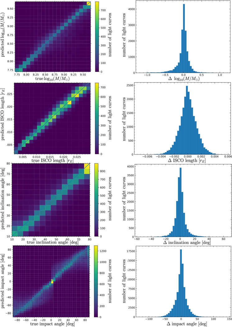
Figure 11: Left: Confusion matrices of the measured against the true values for each parameter for the validation set. The blue line across the diagonal represents a perfect measurement. Right: Histograms of the difference in predicted and true values with mean and standard deviation given in Table 3.

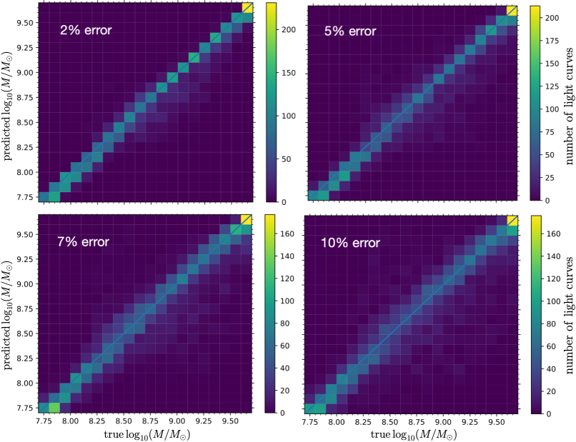
Figure 12: Confusion matrices for the SMBH mass for different photometric errors applied to the input light curves.

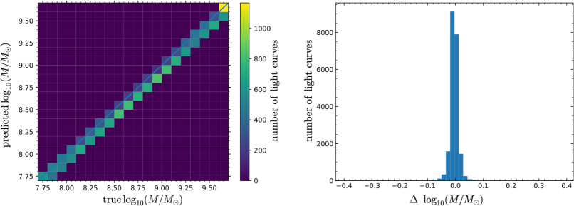
Figure 13: Same as Figure 11 for the black hole mass measured in different bands and redshifts, as indicated in Table 2, with photometric errors simulated for the Gemini telescope. The $1\sigma$ uncertainty is 0.0174 with a bias of -0.0042.

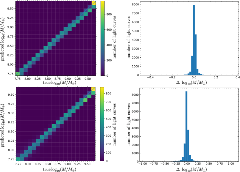
Figure 14: Confusion matrices of test sets. Top: Accretion disk and maximum size held constant based on central black hole mass $10^{8}M_{\odot}$. Bottom: Accretion disk gradient is held constant as calculated for black hole mass $10^{8}M_{\odot}$. The top test has a $1\sigma$ uncertainty of 0.067 with a bias of -0.0011, and the bottom test has uncertainty 0.026 and bias of 0.0013.

4 Results

The ISCO size recovered by the spline and wavelet methods is shown in Figure 10. The second derivative method on average reports the correct ISCO size within one standard deviation, but at the computational cost of needing to search for the proper smoothing factors required to recover it. The wavelet method tends to outperform the second derivative method in some extreme inclinations, as shown in Fig. 9, but often underestimates the proper ISCO size on average as in Fig. 10 by up to 1$\sigma$. At lower signal-to-noise ratios (low $M_{\rm BH}$ and/or high redshift), both methods start to fail: at redshift 1.5 the ISCO of black hole masses with $<10^{8}$ M_⊙ becomes too small to be correctly measured, while at redshift 2.0 this threshold becomes $10^{8.2}$ M_⊙ and redshift 3.0 it is $10^{8.4}$ M_⊙.

The results of the four neural networks, one for each parameter of interest, are shown in Fig. 11. The confusion matrices and accuracy are given once the loss function of the validation set becomes sufficiently flat, causing the training to stop. The confusion matrices are fairly diagonal, meaning that the network does not suffer from any major systematic biases. The uncertainty and accuracy of our predictions is given in Table 3.

In Fig. 12 we show the confusion matrices for predicted mass for four different values of photometric noise levels as an example to emphasise how one prediction can be impacted by an increase in photometric uncertainty. Even with a signal-to-noise ratio of 10, the neural network is still able to make fairly accurate predictions. The $1\sigma$ uncertainty of our prediction of $\log_{10}(M/M_{\odot})$ goes from 0.10 at 2% Gaussian error to 0.24 at 10% Gaussian error. Other parameters were also tested with increased photometric noise, and were found to have similar degradation in predictions.

We also employed the machine learning regression on mock light curves with realistic photometric noise, as outlined in Section 2.3. We test our method on a total of $\sim$100,000 light curves which included four optical bands and five different redshifts within one data set- the full parameter space is given in Table 2 and the results for the black hole mass are shown in Fig. 13. We chose to commit additional resources to these more realistic light curves and doubled their resolution compared to the nominal data sets. As such, the parameters of the network almost doubled to 87,393. The statistical error on the measurement of $\log_{10}(M/M_{\odot})$ is only $\pm 0.002$. This very high accuracy is due to the much higher signal-to-noise ratio ranging from $\sim 50$ to 100 in these simulations, dependent on redshift and band. The different photometric error between optical bands does not make much of a difference in the machine learning results, with the z band performing slightly worse due to its overall lower signal-to-noise ratio.

prediction	range	bias	uncertainty
$\log_{10}(M/M_{\odot})$	7.7 to 9.7	-0.006	0.185
ISCO width [$r_{E}$]	0 to 0.03	0.00004	0.00126
Inclination angle	10$\degree$ to 80$\degree$	0.14$\degree$	7.39$\degree$
Impact angle	-80$\degree$ to 80$\degree$	-0.58$\degree$	17.9$\degree$

Table 3: Bias and $1\sigma$ uncertainties across the validation set in each networks’ predictions.

5 Discussion and conclusions

We have developed simulations of strongly-lensed quasar accretion disks under caustic-crossing microlensing events, including a fully relativistic disk model, a high-resolution magnification map created through inverse ray-tracing, and a realistic noise model. We have analyzed the resulting light curves to measure features of the inner accretion disk assuming follow-up observations with high cadence and high signal-to-noise ratio. Our simulations assume an isolated caustic structure, resulting mostly from a single microlens with some external shear. While this may be idealized, we note that some such events are expected to be observed in the hundreds to thousands of caustic-crossing events to be detected by LSST (Neira et al., 2020).

For near face-on accretion disks where relativistic effects are nearly insignificant, the ISCO manifests as a  1% to 10% dip in brightness as the caustic crosses it, resulting in a double-peak structure in the light curve. This dip can last anywhere from days to months depending on the transverse velocity, lens, source, and physical size of the ISCO. For a moderately to highly inclined accretion disk, relativistic effects lead to a highly asymmetric light curves near the ISCO crossing.

Analyzing the ISCO-crossing feature using the second derivative of a spline fit and a wavelet decomposition gives us a direct estimate of the projected ISCO width. These methods are sensitive to the choice of certain parameters, such as the order of the spline/wavelet used and thresholds for ISCO edge detection. When paired with human judgement, these are effective methods of measuring the ISCO width, but more work is needed to create a robust algorithm.

We note that projected ISCO width is a function of several parameters, such as the SMBH mass and spin, as well as the inclination angle of the accretion disk with respect to our line of sight.

We also train a convolutional neural network to predict various physical parameters from an input caustic-crossing light curve, including black hole mass, inclination angle, and ISCO width. Applying our trained CNN to a test sample of light curves generated from a wide range of these physical parameters, we find that it predicts mass and inclination angle remarkably well. With simulated light curves of high signal-to-noise ratio and redshift within this range, predictions of mass are comparable to those of reverberation mapping. The CNN also predicts the inclination angle for this test sample to within 10$\degree$. There are currently few methods for constraining AGN orientation, so this result is potentially very exciting.

In comparison to the spline and wavelet methods, the neural network measures the black hole mass significantly more precisely. The CNN measurements are also found to be more accurate as seen in the histograms in Figures 11, 13, and 14.

Overall, the CNN outperforms these classical analytic methods for determining the ISCO size in caustic-crossing events. Both methods perform well for high signal-to-noise photometry, though the CNN has the added benefit of requiring much less human judgement.

We find that monitoring of a caustic-crossing event by a quasar’s inner accretion disk enables the measurement of a variety of properties in the vicinity of the SMBH, with excellent precision obtained for $\sim$5% photometry or better. The observational cadence depends greatly on the microlensing parameters. Our results show reasonable predictions down to $\sim$2 observations per week in multiple optical bands over the full duration of the caustic-crossing event if a low effective velocity is assumed. We do not expect LSST to provide sufficient cadence across all bands to adequately sample the ISCO crossing, however we do expect it to be able to provide the trigger necessary for multi-platform followup of the caustic-crossing event.

6 Acknowledgements

This research was made possible by the generosity of Eric and Wendy Schmidt by recommendation of the Schmidt Futures program. Error simulated is based on observations obtained at the international Gemini Observatory, a program of NSF’s NOIRLab, which is managed by the Association of Universities for Research in Astronomy (AURA) under a cooperative agreement with the National Science Foundation on behalf of the Gemini Observatory partnership: the National Science Foundation (United States), National Research Council (Canada), Agencia Nacional de Investigación y Desarrollo (Chile), Ministerio de Ciencia, Tecnología e Innovación (Argentina), Ministério da Ciência, Tecnologia, Inovações e Comunicações (Brazil), and Korea Astronomy and Space Science Institute (Republic of Korea).

In addition to user created code, the following Python modules were also used: Numpy, Scipy, Astropy, Matplotlib, Tensorflow/Keras, and PyWavelets. These resources have been invaluable to both creating and exploring the data simulations. GYOTO code and the GERLUMPH database were also extraordinarily helpful to the creation of data sets and the microlensing simulations.

References

- Abajas et al. (2002) Abajas C., Mediavilla E., Muñoz J. A., Popović L. Č., Oscoz A., 2002, ApJ, 576, 640
- Abolmasov & Shakura (2012) Abolmasov P., Shakura N. I., 2012, MNRAS, 423, 676
- Agol & Krolik (1999) Agol E., Krolik J., 1999, ApJ, 524, 49
- Anguita et al. (2008) Anguita T., Schmidt R. W., Turner E. L., Wambsganss J., Webster R. L., Loomis K. A., Long D., McMillan R., 2008, A&A, 480, 327
- Antonucci (1993) Antonucci R., 1993, ARA&A, 31, 473
- Bañados et al. (2018) Bañados E., et al., 2018, Nature, 553, 473
- Bate et al. (2008) Bate N. F., Floyd D. J. E., Webster R. L., Wyithe J. S. B., 2008, MNRAS, 391, 1955
- Bate et al. (2018) Bate N. F., et al., 2018, Monthly Notices of the Royal Astronomical Society, 479, 4796
- Blackburne et al. (2011) Blackburne J. A., Pooley D., Rappaport S., Schechter P. L., 2011, ApJ, 729, 34
- Blackburne et al. (2014) Blackburne J. A., Kochanek C. S., Chen B., Dai X., Chartas G., 2014, ApJ, 789, 125
- Blackburne et al. (2015) Blackburne J. A., Kochanek C. S., Chen B., Dai X., Chartas G., 2015, ApJ, 798, 95
- Cackett et al. (2021) Cackett E. M., Bentz M. C., Kara E., 2021, iScience, 24, 102557
- Daubechies (1988) Daubechies I., 1988, Communications on pure and applied mathematics, 41, 909
- Dexter et al. (2010) Dexter J., Agol E., Fragile P. C., McKinney J. C., 2010, ApJ, 717, 1092
- Event Horizon Telescope Collaboration et al. (2019) Event Horizon Telescope Collaboration et al., 2019, ApJ, 875, L1
- Fluke & Webster (1999) Fluke C. J., Webster R. L., 1999, MNRAS, 302, 68
- Gravity Collaboration et al. (2017) Gravity Collaboration et al., 2017, A&A, 602, A94
- Grieger et al. (1988) Grieger B., Kayser R., Refsdal S., 1988, A&A, 194, 54
- Hutsemekers et al. (1994) Hutsemekers D., Surdej J., van Drom E., 1994, Ap&SS, 216, 361
- Jiménez-Vicente et al. (2012) Jiménez-Vicente J., Mediavilla E., Muñoz J. A., Kochanek C. S., 2012, ApJ, 751, 106
- Jiménez-Vicente et al. (2014) Jiménez-Vicente J., Mediavilla E., Kochanek C. S., Muñoz J. A., Motta V., Falco E., Mosquera A. M., 2014, ApJ, 783, 47
- Kelly et al. (2010) Kelly B. C., Vestergaard M., Fan X., Hopkins P., Hernquist L., Siemiginowska A., 2010, The Astrophysical Journal, 719, 1315–1334
- Kerr (1963) Kerr R. P., 1963, Phys. Rev. Lett., 11, 237
- Kingma & Ba (2017) Kingma D. P., Ba J., 2017, Adam: A Method for Stochastic Optimization (arXiv:1412.6980)
- Kochanek (2004) Kochanek C. S., 2004, ApJ, 605, 58
- Lee et al. (2019) Lee G. R., Gommers R., Waselewski F., Wohlfahrt K., O’Leary A., 2019, Journal of Open Source Software, 4, 1237
- Lewis & Belle (1998) Lewis G. F., Belle K. E., 1998, MNRAS, 297, 69
- Mallat (2008) Mallat S., 2008, in A Wavelet Tour of Signal Processing, Third Edition: The Sparse Way.
- McConnell & Ma (2013) McConnell N. J., Ma C.-P., 2013, ApJ, 764, 184
- Mediavilla et al. (2015) Mediavilla E., Jiménez-vicente J., Muñoz J. A., Mediavilla T., 2015, The Astrophysical Journal, 814, L26
- Morgan et al. (2010) Morgan C. W., Kochanek C. S., Morgan N. D., Falco E. E., 2010, ApJ, 712, 1129
- Morgan et al. (2018) Morgan C. W., Hyer G. E., Bonvin V., Mosquera A. M., Cornachione M., Courbin F., Kochanek C. S., Falco E. E., 2018, ApJ, 869, 106
- Mortlock et al. (2011) Mortlock D. J., et al., 2011, Nature, 474, 616
- Mortonson et al. (2005) Mortonson M. J., Schechter P. L., Wambsganss J., 2005, ApJ, 628, 594
- Mosquera & Kochanek (2011) Mosquera A. M., Kochanek C. S., 2011, The Astrophysical Journal, 738, 96
- Muñoz et al. (2016) Muñoz J. A., Vives-Arias H., Mosquera A. M., Jiménez-Vicente J., Kochanek C. S., Mediavilla E., 2016, The Astrophysical Journal, 817, 155
- Nair & Hinton (2010) Nair V., Hinton G. E., 2010, in Proceedings of the 27th International Conference on International Conference on Machine Learning. ICML’10. Omnipress, Madison, WI, USA, p. 807–814
- Neira et al. (2020) Neira F., Anguita T., Vernardos G., 2020, Monthly Notices of the Royal Astronomical Society, 495, 544–553
- O’Dowd et al. (2011) O’Dowd M., Bate N. F., Webster R. L., Wayth R., Labrie K., 2011, MNRAS, 415, 1985
- Oguri & Marshall (2010) Oguri M., Marshall P. J., 2010, Monthly Notices of the Royal Astronomical Society, p. no–no
- O’Dowd et al. (2015) O’Dowd M. J., Bate N. F., Webster R. L., Labrie K., Rogers J., 2015, The Astrophysical Journal, 813, 62
- Padovani et al. (2017) Padovani P., et al., 2017, A&ARv, 25, 2
- Paic et al. (2021) Paic E., Vernardos G., Sluse D., Millon M., Courbin F., Chan J. H., Bonvin V., 2021, Constraining quasar structure using high-frequency microlensing variations and continuum reverberation (arXiv:2110.05500)
- Pooley et al. (2007) Pooley D., Blackburne J. A., Rappaport S., Schechter P. L., 2007, ApJ, 661, 19
- Salpeter (1964) Salpeter E. E., 1964, ApJ, 140, 796
- Schneider & Wambsganss (1990) Schneider P., Wambsganss J., 1990, A&A, 237, 42
- Shakura & Sunyaev (1973) Shakura N. I., Sunyaev R. A., 1973, Astronomy and Astrophysics, 500, 33
- Sluse et al. (2007) Sluse D., Claeskens J. F., Hutsemékers D., Surdej J., 2007, A&A, 468, 885
- Sluse et al. (2011) Sluse D., et al., 2011, A&A, 528, A100
- Thompson et al. (2010) Thompson A. C., Fluke C. J., Barnes D. G., Barsdell B. R., 2010, New Astron., 15, 16
- Tomozeiu et al. (2016) Tomozeiu M., Mohammed I., Rabold M., Saha P., Wambsganss J., 2016, Microlensing as a possible probe of event-horizon structure in quasars (arXiv:1604.01769)
- Vernardos & Tsagkatakis (2019) Vernardos G., Tsagkatakis G., 2019, Monthly Notices of the Royal Astronomical Society, 486, 1944–1952
- Vincent et al. (2011) Vincent F. H., Paumard T., Gourgoulhon E., Perrin G., 2011, Classical and Quantum Gravity, 28, 225011
- Wambsganss (2006) Wambsganss J., 2006, Gravitational Lensing: Strong, Weak and Micro, p. 453–540
- Wambsganss & Paczynski (1991) Wambsganss J., Paczynski B., 1991, AJ, 102, 864
- Williams et al. (2021) Williams P. R., et al., 2021, The Astrophysical Journal, 911, 64
- Wyithe et al. (2002) Wyithe J. S. B., Agol E., Fluke C. J., 2002, MNRAS, 331, 1041
- Zel’dovich (1964) Zel’dovich Y. B., 1964, Soviet Physics Doklady, 9, 195