Probing the Singularities of the
Landau-Gauge Gluon and Ghost Propagators
with Rational Approximants

Abstract

We employ Padé approximants in the study of the analytic structure of the four-dimensional $SU(2)$ Landau-gauge gluon and ghost propagators in the infrared regime. The approximants, which are model independent, serve as fitting functions for the lattice data. We carefully propagate the uncertainties due to the fitting procedure, taking into account all possible correlations. For the gluon-propagator data, we confirm the presence of a pair of complex poles at $p_{\rm pole}^{2}=\left[(-0.37\,\pm\,0.05_{\rm stat}\,\pm\,0.08_{\rm sys})\pm i\,(0.66\,\pm\,0.03_{\rm stat}\,\pm\,0.02_{\rm sys})\right]\,\mathrm{GeV}^{2}$, where the first error is statistical and the second systematic. The existence of this pair of complex poles, already hinted upon in previous works, is thus put onto a firmer basis, thanks to the model independence and to the careful error propagation of our analysis. For the ghost propagator, the Padés indicate the existence of a single pole at $p^{2}=0$, as expected. In this case, our results also show evidence of a branch cut along the negative real axis of $p^{2}$. This is corroborated with another type of approximant, the D-Log Padés, which are better suited to studying functions with a branch cut and are applied here for the first time in this context. Due to particular features and limited statistics of the gluon-propagator data, our analysis is inconclusive regarding the presence of a branch cut in the gluon case.

1 Introduction

The low-momentum behavior of Green functions in Yang-Mills theory for different gauges has been an important subject of study for the past 40 years or so, mainly in connection with the understanding of the color-confinement property of QCD [1, 2, 3, 4]. The topic is treated both by analytic and numerical methods, all of which involve significant technical challenges. In particular, most studies have focused on the Landau-gauge case, giving rise to several theoretical advances and proposals, with lively debate between researchers using different approaches [5].

Concerning lattice simulations of Green functions, the main numerical difficulty is somewhat unusual. Indeed, in typical lattice-QCD applications, one just needs to consider a large enough discretized volume to ensure a physical lattice side $L$ a few times greater than the relevant hadronic scale ($\approx 1\leavevmode\nobreak\ \text{fm}$). This stems from the fact that finite-size corrections affecting hadronic observables are suppressed by a factor of $\exp{(-m_{\pi}L)}$ [6], where $m_{\pi}$ is the lattice pion mass. The effort, then, is to go to very small lattice spacing ($\lesssim 0.1\leavevmode\nobreak\ \text{fm}$), in order to avoid discretization errors. In studies of the infrared (IR) region, however, the situation is different. This happens because the IR limit, which corresponds to small momenta, requires a large lattice side $L$. In fact, the smallest nonzero momentum that can be represented on a lattice is $\approx 2\pi/L$. As it turns out, for the Landau-gauge gluon and ghost propagators, finite-size effects are particularly severe [7, 8, 9, 10, 11, 12, 13, 14] (see also Ref. [15] and references therein), implying that one needs data at momenta $p$ well below $300\leavevmode\nobreak\ \text{MeV}$ in order to obtain a clear picture of the IR region. The low-momentum behavior of the gluon and ghost propagators is a central prediction of different theoretical frameworks — or scenarios — for understanding the confinement mechanism. Early on, the lack of control over finite-size effects in simulations has obscured the true qualitative behavior of these propagators in the deep IR region. This has been settled by later studies [5]. Nevertheless, present lattice data still accommodate descriptions based on rather different analytic predictions [16, 11, 17, 18, 19, 20]. On the contrary, violation of reflection positivity in the real-space gluon propagator, which may be claimed to be a signal of color confinement [1, 2, 3, 4], has been a directly observed feature since early simulations [21, 22, 23]. Recently, the focus has switched from testing specific analytic predictions to the investigation of the analytic structure of the IR gluon and ghost propagators, more or less independently of the various scenarios. In particular, the main effort has been in identifying the dominant singularities (poles, branch cuts) in the complex plane. This usually involves either direct analytic studies using complex momenta [24, 25, 26, 27, 28, 29] or an analytic continuation of the Euclidean Green functions by different methods [30, 31, 32, 33, 34, 35, 36], guided by general properties of the Källén-Lehmann spectral density.

The use of rational (or Padé) approximants provides a model-independent route to attack this problem. Recently, Padé approximants were used to fit $SU(3)$ propagators [37, 38] by Falcão, Oliveira and Silva. Here, we follow this approach to study the analytic structure of the four-dimensional $SU(2)$ Landau-gauge gluon and ghost propagators in the IR regime. More specifically, we carry out a consistent and systematic analysis using Padé approximants (PAs) (and other rational approximants) as fitting functions to the lattice data from Refs. [9, 39, 40, 5, 41, 42]. Let us recall that a Padé approximant $P^{M}_{N}(z)$ is the ratio of two polynomials of degree $M$ (in the numerator) and $N$ (in the denominator). Padé theory [43, 44] then provides us with a systematic procedure to reconstruct a given function, using the same information as its truncated Taylor expansion: the derivatives of the function at a given point in the complex plane, often taken to be the origin. However, note that, compared with the Taylor series — and provided sufficient information about the function is available — Padé approximants are much more powerful. Indeed, they 1) have an extended range of validity, 2) are capable of reproducing the singularities of the original function (poles and residues), and 3) can mimic the existence of branch cuts in the complex plane. Moreover, in certain situations, theorems guarantee the convergence of sequences of approximants to the original function in a given limit, except at the singularities where the function is not well defined. Nevertheless, even when theorems are not available, Padé approximants have been shown in practice to be extremely useful as well [45]. We refer to the procedure of building PAs from the Taylor expansion of a function at a given point as “genuine Padés”. These have found many applications in particle physics (for a few recent ones see Refs. [46, 47, 48, 49, 50, 51, 52, 53, 54, 55]).

Per contra, in the present work, we employ a variant of the above procedure, using rational approximants as fitting functions to (lattice) data, taking advantage of the extended range of validity of the Padé approximants compared to the Taylor expansion. This procedure departs from the genuine Padés but it has been successfully used in several applications to experimental data [56, 57, 58, 59, 60, 61], as well as to $SU(3)$ lattice data for Landau-gauge propagators [37, 38]. In fact, using rational approximants as fitting functions can be a powerful method, especially in situations where the precise theoretical description of the data is not feasible or is model dependent. In particular, the use of sequences of approximants provides a model-independent way of extracting crucial information, such as resonance poles in scattering amplitudes or the Taylor expansion of hadronic form factors. Here, we aim at extracting information about the analytic structure of the Landau-gauge gluon and ghost propagators.

We point out that a popular confinement scenario proposes for the IR gluon propagator a form that can be cast as a Padé approximant. Indeed, the Gribov-like [62] (or Stingl-like [63, 64]) function $f_{1}(p^{2})$ of Ref. [41] belongs to the Padé sequence $P_{N+1}^{N}(p^{2})$ (for $N=1$). Here we do not assume any specific rigid form for the propagators, but rather we explore their properties by a systematic investigation of different Padé sequences, in a model-independent way. As said above, a first analysis of the singularities of the $SU(3)$ Landau-gauge gluon and ghost propagators using rational approximants was presented in Refs. [37, 38]. In their work, the authors found evidence for the existence of a pair of complex poles in the gluon propagator and of a simple pole at zero momentum in the ghost-propagator data. At the same time, their results seem to support the presence of a branch cut — along the negative real axis of the Euclidean $p^{2}$ momenta — for both propagators. Similar outcomes are obtained in Ref. [32] for gluon and ghost propagators, both in Landau gauge and in linear covariant gauge, using a related approach.

Although our analysis and that of Refs. [37, 38] are very similar in spirit, there are a few important differences. Firstly, we consider $SU(2)$ lattice-gauge-theory data [9, 39, 40, 5, 41], whereas the authors of Refs. [37, 38] analyzed gluon and ghost propagators in the $SU(3)$ case. (We recall, however, that the propagators are very similar for these two gauge groups in the IR limit, not only qualitatively but also quantitatively [65, 66, 67].) Secondly, we perform a careful analysis of the uncertainties involved in the fitting procedure. Note that this is especially relevant for results from PAs with many parameters, since these are likely affected by uncontrolled errors, thus compromising the reliability of the final results for the analytic structure of the propagators in the complex plane. Indeed, since we use Padé approximants as fitting functions, a $\chi^{2}$ fit procedure is clearly required, and the uncertainties in the parameters of the fit must be carefully examined. Moreover, the errors have to be propagated to all related results, including the position of zeros and poles in the complex plane. Consequently, these uncertainties, which ultimately reflect the information available in the data set, restrict the number of parameters that can be reliably obtained in a given fit, thus imposing limits on the order of the approximants $P_{N}^{M}(z)$ that can be employed in practice. In particular, we will see that, for the data sets we have, our analysis is limited to PAs of relatively low order (up to 10 parameters). In the present study, all uncertainties in the fits to data are carefully calculated (with more than one method), including all correlations when necessary, and the limitations they impose on our analysis are discussed in detail.

This paper is organized as follows. In Sec. 2 we give an overview of Padé theory with emphasis on the present application. In Sec. 3 we discuss the use of the approximants to analyze a toy data set, in order to check the applicability of our approach. In Sec. 4 the details of the lattice simulation and of the lattice data considered here are briefly described. Our results are given in Sec. 5, with Sec. 5.1 devoted to the application of PAs to the Landau-gauge gluon propagator, and Sec. 5.2 to applications to the ghost propagator using PAs and partial PAs, obtained by imposing the existence of the pole at zero momentum. For the ghost propagator we also consider in Sec. 5.2.1 the use of D-Log Padé approximants [44, 53, 54], a variant of the method better suited for the application to functions that present a branch cut. Our conclusions are given in Sec. 6. Some technical details on fits for highly-correlated data, and in particular a short description of the so-called “diagonal fits”, are reported in Appendix A. In Appendix B, we briefly discuss the issue of numerical precision when using higher-order Padé approximants.

2 Rational approximants

In this section we introduce the most important concepts about Padé approximants, with emphasis on the problem we have at hand. A much more comprehensive discussion, including the demonstration of theorems, can be found in the works by Baker and Graves-Morris [43, 44] (see also Ref. [45] for several applications in particle physics).

The Padé approximant, $P_{N}^{M}(z)$, is defined as the ratio of the polynomials of order $M$ and $N$, $Q_{M}(z)$ and $R_{N}(z)$, respectively, with $R_{N}(0)=1$:

$$P_{N}^{M}(z)=\dfrac{Q_{M}(z)}{R_{N}(z)}=\dfrac{a_{0}+a_{1}\,z+\cdots+a_{M}\,z^{M}}{1+b_{1}\,z+\cdots+b_{N}\,z^{N}}\;.$$ (1)

If the Taylor series of a function $f(z)$ is known, the canonical procedure to build PAs to this function is to determine the coefficients $a_{k}$ and $b_{k}$ by matching the expansion of $P^{M}_{N}(z)$ to the first $M+N+1$ coefficients of the Taylor expansion of $f(z)$.

In Padé theory, convergence theorems are available for analytic and single-valued functions with multipoles or even essential singularities [44]. A class of functions that play a prominent role are the Stieltjes functions, which can be written in integral form as

$$f(z)=\int\displaylimits_{0}^{\infty}\dfrac{\mathrm{d}\phi(u)}{1+zu}\;,$$ (2)

where $\phi(u)$ is a (non-negative) measure on $[0,\infty)$. Indeed, for $f(z)$, the Padé sequences $P_{N}^{N+k}(z)$, with $k\geq-1$, converge to Stieltjes functions, with some interesting properties. One of them is that the poles of these Padés are always simple and are located on the negative real axis of $z$ with positive residues [44]. The connection with the present work is obvious from the Källén-Lehmann representation of propagators, in terms of positive-definite spectral functions. As we will see, the Padés to the gluon propagator $D(p^{2})$ have poles with an imaginary part incompatible with zero, which is in contradiction with the usual Källén-Lehmann representation for $D(p^{2})$ [68, 69]. Following Ref. [29], this would also imply the existence of several branch cuts for the gluon and ghost propagators, and the consequent violation of the Källén-Lehmann representation (see also Ref. [27]) for the ghost propagator $G(p^{2})$. (For general discussions of the analytic structures of these propagators see also Refs. [70, 33, 34].) This suggests that an integral representation for the gluon and ghost propagators is only possible if the function is not Stieltjes, i.e. if one considers some modified spectral representation [32, 36, 29].

Another important result from Padé theory that will guide our work is related to Pommerenke’s theorem, which states that a sequence of approximants $P^{N}_{N+k}(z)$ — built for a meromorphic function $f(z)$ — converges in any compact set of the complex plane [except for a set of zero area containing the poles of $f(z)$]. Indeed, as $N$ increases, the poles of $f(z)$ are well reproduced by the PAs and tend to be stable, i.e. they remain unchanged (or almost unchanged) when $N$ is increased. At the same time, extraneous poles can also appear in the PAs, but they either go away when the order is increased or they appear in combination with a nearby zero, which leads to a very small residue, partially cancelling the effects of the pole. The latter case corresponds to the so-called Froissart doublets, which do not represent genuine poles of $f(z)$. Note that the appearance of transient Froissart doublets may “delay” the convergence of a Padé sequence to a function, since they effectively reduce the order of the approximant [53, 54]. Nevertheless, Padé approximants that have doublets can still be used to approximate the function away from these singularities.

Functions with branch points and cuts can also be approximated by PAs, although for such functions the expected convergence is mainly motivated by experience and not by theorems. In this case, the approximants will mimic a cut of a given function by accumulating poles (interleaved with zeros) along the cut in the complex plane [44, 45, 71]. Since the gluon and ghost propagators are expected to have a cut [37, 38, 29], this will be of relevance here.

As said in the Introduction, we use the PAs as fitting functions to describe (lattice) data sets. The advantages of this procedure are 1) its model independence, 2) the fact that it can be applied in a systematic way, and 3) the connection with Padé theory (although here no theorems are available). This type of application is quite common in other particle-physics problems for which the theoretical description of the data is model dependent or incomplete [56, 57, 49, 59, 60, 61, 50]. An application that is particularly close to ours is the extraction of resonance poles, using the PAs as fitting functions to decay, scattering or form-factor data [49, 50, 61]. Indeed, it has been shown that the use of PAs as fitting functions is a reliable and model-independent method to determine resonance pole positions from fits to data sets. The precision of this procedure is obviously limited by the quality of the data set: with larger errors, less information is available and, eventually, adding more parameters — i.e. increasing the order of the PA in the sequence — is no longer an advantage, since the errors of the parameters (and of the pole positions) increase considerably. In some applications, it has been found that the maximum number of parameters that can be meaningfully extracted from a data set was 6 or 7, which limits the PAs of the $P_{N}^{N}(z)$ sequence to $N=3$, for instance [49]. We will show that, with our lattice data for the gluon propagator, the situation is very similar: it hardly makes sense to have more than 6 or 7 parameters in the PAs. Likewise, for the ghost data, we were able to consider at most 7 or 8 parameters in the Padé approximants. Of course, with increased statistics, one expects that more parameters would be allowed and that fits with higher-order PAs would be meaningful as well.

3 Conceptual examples

Before applying the procedure to the real lattice data, it is useful to test the method in a fully controlled setting, i.e. applied to a function whose analytic structure is known. This is especially important here, since the application of PAs as fitting functions is beyond the reach of the theorems of Padé theory. We start by building genuine PAs, from the exact knowledge of the Taylor series of the chosen function. Then, we generate a toy data set, following the main features of the lattice data we will analyze in the next sections. Similar tests with toy data sets were also carried out in Ref. [37].

For the present analysis, we choose a function that has as many features as possible — poles, a branch cut, as well as zeros — in order to mimic a sufficiently realistic scenario. To this end, we employ the function

$$g(z)=1.15\,\log{(z+2)}\,\,\dfrac{z+2.508}{z^{2}+0.768^{2}\,z+0.72^{2}}\;,$$ (3)

which roughly resembles the lattice data for the gluon propagator. In fact, this function has a pair of complex poles at $z_{0}=-0.295\pm 0.657\,i$, two zeros (located at $z=-1$ and $z=-2.508$) and a branch cut from $(-\infty,-2]$, similarly to the results presented in Ref. [41]. Thus, it captures the main features of models that describe the gluon propagator in the infrared, such as a branch cut and complex poles [32, 37, 38, 29]. Note that this function is a product of a Stieltjes function, $\log(z+2)$, with a rational meromorphic function. Therefore, the appearance of complex Froissart doublets is not expected in its approximation by PAs [43, 44].

We start by building genuine PAs to the Taylor expansion of $g(z)$ around $z=0$. By applying PAs from the diagonal and near-diagonal sequences $P_{N}^{N}(z)$, $P_{N+1}^{N}(z)$ and $P_{N}^{N+1}(z)$, a number of features is evident. In particular, the reproduction of the analytic aspects is hierarchical. Indeed, the pair of complex poles and the zero closer to the origin are already replicated by PAs of lower order ($N=2$ or 3), while the second zero (at $z=-2.508$), which is further away from the origin, is reproduced only by PAs with more parameters. This is expected, since poles and zeros closer to the origin are usually reproduced first. At the same time, the PAs also mimic the cut by accumulating (artificial) poles interleaved with zeros along the branch cut. This, however, requires many parameters and is salient only when a large number of parameters is available. Furthermore, the position of the first pole of this type tends to approach the branch point but, again, it only leads to a good reproduction of the branch point if sufficiently many parameters are available.

(a)

(b)

Figure 1: (a) Poles (filled circles) and zeros (empty squares) of $P_{15}^{14}(z)$ built to the Taylor series of $g(z)$ defined in Eq. (3). The poles and zeros that can be identified with genuine poles of $g(z)$ are shown in green, while artifacts are shown in red (poles) and blue (zeros). (b) Real and imaginary parts of the complex poles $z_{0}^{\rm PA}$ (normalized to their true values) for the sequences $P_{N}^{N}(z)$ and $P_{N+1}^{N}(z)$, as a function of the number of parameters of the PA. To avoid inaccurate numerical results for the higher-order PAs (see Appendix B), the results in this figure were obtained working with 30 decimal places.

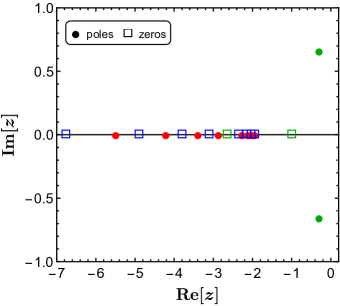
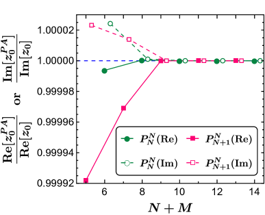
To be concrete, in Fig. 1a, we show the analytic structure of a typical higher-order PA, $P^{14}_{15}(z)$. The green circles show the pair of complex poles, which can easily be identified with the true poles of $g(z)$ (we refer to these poles as “physical”). The green squares show the zeros of $g(z)$, whereas red circles and blue squares represent artificial (or “non-physical”) poles and zeros, respectively. The main characteristic of the physical poles and zeros is the fact that they are stable, i.e. they remain essentially fixed as $N$ increases. The impressive convergence of the pole position obtained from the PAs to the correct value is shown as a function of $N+M$ in Fig. 1b, where we display the real and imaginary parts of the physical poles of the PAs (normalized to the exact values). Finally, poles and zeros start to accumulate along the branch cut with branch point $z=-2$, where the PA places a pole. We stress that these results are expected when using genuine PA approximants, but one should nonetheless verify if this also happens when the PAs are used as fitting functions. Finally, it is important to mention that when constructing Padé approximants of higher order, such as $P^{14}_{15}(z)$ of Fig. 1a, the precision of the numerical solution becomes crucial. If insufficient precision is used, artificial (incorrect) pairs of complex poles with very small residues, resembling Froissart doublets, displaying a roughly semi-circular pattern in the complex plane, can appear in the approximant (see Ref. [72] and the discussion in Appendix B).

Next, in order to investigate the use of PAs as fitting functions, as well as to test our fit procedure, we built a toy data set for $g(z)$ with 400 data points, for every value of $z$ between 0.01 and $4$ in steps of 0.01. We generate these data using a Gaussian distribution around the value of $g(z)$ with 1% error, which is in the ballpark of the errors we have in our lattice data. The parameters of the PA are then obtained from a $\chi^{2}$ fit to the toy data. The errors of the parameters were estimated with four different methods: Hessian matrix, Monte Carlo error propagation, $\Delta\chi^{2}$ variation (see, for example, the Particle Data Group review on Statistics [73]), and a linear error propagation (discussed in Appendix A). In all cases the errors we obtain from the four methods are in good agreement. A few observations are, however, in order. If the number of parameters exceeds $8$ or so, the statistical uncertainties grow dramatically and the fit parameters are not meaningful anymore. Consequently, since the errors propagate to pole positions and zeros, these become equally meaningless. The bottom line is that, with our toy data set, which is similar to our real lattice data, we must limit the number of parameters in the PA to at most 8 or 9. (These conclusions also apply to fits to the real data, as we discuss further below.) An important point about the toy data is that, due to statistical fluctuations, we can no longer guarantee that no complex Froissart doublets will appear (see e.g. Ref. [72]), even though the underlying function is a product of a Stieltjes function with a meromorphic function.

(a)

(b)

Figure 2: (a) Poles (filled circles) and zeros (empty squares) of $P_{4}^{3}(z)$ fitted to the toy data set generated from $g(z)$, Eq. (3). The poles and zeros that can be identified with genuine poles of $g(z)$ are in green, while artifacts are shown in red (poles) and blue (zeros). (b) Real and imaginary parts of the complex pole $z_{0}^{\rm PA}$ predicted by the PAs, normalized to their corresponding true value, for approximants belonging to the sequences $P_{N}^{N}(z)$ and $P_{N+1}^{N}(z)$, as a function of the number of parameters of the PA.

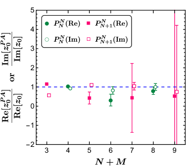
In Fig. 2a we show the analytic structure of the PA $P^{3}_{4}(z)$, with 8 parameters, built to the considered data set. In green, we see that the PA reproduces the poles of $g(z)$, albeit not very precisely, and places a zero that can be identified with the true zero at $z=-1$. A Froissart doublet is also clearly seen, as well as a pole and a zero along the real axis, which could be the beginning of the manifestation of the branch cut. In Fig. 2b we show the behavior of the pole position with increasing values of $N$. We see that the pole is relatively stable, which is very important to identify it as a physical one. Furthermore, it is clear that lower values of $N$ can, in fact, be advantageous, since they lead to smaller errors in the pole position. Finally, for more than 8 or 9 parameters, the errors on the pole position are so large that the results are no longer meaningful.

This analysis shows that using the PAs as fitting functions is also a reliable method to extract the main features of the analytic structure of $g(z)$. However, the limitations imposed by the data errors are evident: we cannot go to very high orders in the Padé sequences, and the reproduction of pole positions and zeros has uncertainties stemming from the fit parameters. These errors must be carefully propagated, and grow significantly once the order of the PA is larger than $8$ or $9$. In particular, in this situation, it becomes difficult to see the footprints of the branch cut, which would require a larger number of parameters.

4 Lattice data for the Landau-gauge propagators

The data for the (four-dimensional) $SU(2)$ Landau-gauge gluon and ghost propagators used in the present work have been previously presented and discussed in Refs. [9, 39, 40, 5, 41, 42], which contain technical details of the simulations. Here, we recall the main parameters and properties that are relevant for our analysis.

We have considered symmetric lattices with various lattice sides, allowing us to keep finite-size effects under control. In the following, we use only the data from our largest lattice volume, $V=n^{4}=128^{4}$, which can be essentially considered as infinite volume. The lattice parameter was taken to be $\beta=2.2$. This yields, approximately, a lattice spacing $a$ of $0.210\leavevmode\nobreak\ \text{fm}$, obtained by considering the input value $\sigma^{1/2}=0.44\leavevmode\nobreak\ \text{GeV}$ for the string tension [74]. The resulting physical lattice volume is about $(27\leavevmode\nobreak\ \text{fm})^{4}$, which is clearly much larger than a typical hadronic scale. Correspondingly, the smallest non-zero (physical) momentum $p_{min}=2\,a^{-1}\sin(\pi/n)$ allowed is about $46\leavevmode\nobreak\ \text{MeV}$.

The lattice gluon propagator $D(p^{2})$ in Landau gauge is evaluated using

$$D^{bc}_{\mu\nu}(p)\;=\;\sum_{x\mbox{,}\,y}\frac{e^{-2\pi i\hat{p}\cdot(x-y)/n}}{V}\,\langle A^{b}_{\mu}(x)\,A^{c}_{\nu}(y)\rangle\;=\;\,\delta^{bc}\,\left(g_{\mu\nu}\,-\,\frac{p_{\mu}\,p_{\nu}}{p^{2}}\right)D(p^{2})\;.$$ (4)

Here, $\langle\;\;\rangle$ stands for the path-integral average, $x,y$ are lattice points, $\mu,\nu$ correspond to Lorentz indices, and $b,c$ to color indices. Also, $A_{\mu}(x)$ is the lattice gluon field, defined as $A_{\mu}(x)=[U_{\mu}(x)-U_{\mu}^{\dagger}(x)]/(2i)$, where $U_{\mu}(x)$ are the usual link variables of the Wilson action. Note that, with this definition, the gluon propagator evaluated on the lattice corresponds to the propagator $g^{2}D(p^{2})$ in the continuum [75]. As for the ghost propagator $G(p^{2})$, it is obtained by inverting the Landau-gauge lattice Faddeev-Popov matrix ${\cal M}(b,x;c,y)$ — for example, defined in Eq. (22) of Ref. [76] — through the relation

$$G^{bc}(p^{2})\,=\,\sum_{x\mbox{,}\,y}\frac{e^{-2\pi i\,\hat{p}\cdot(x-y)/N}}{V}\,\langle\,{\cal M}^{-1}(b,x;c,y)\,\rangle\;=\;\,\delta^{bc}\,G(p^{2})\;,$$ (5)

where $b$ and $c$ are again color indices. For the data considered here, the matrix ${\cal M}(b,x;c,y)$ was inverted by using a conjugate-gradient method with even/odd preconditioning and point sources [77, 78].

For the ghost propagator $G(p^{2})$, the data are displayed [42] simply as a function of the (unimproved) lattice momenta

$$p^{2}\,=\,\sum_{\mu}\,p_{\mu}^{2}\;,$$ (6)

with the components $p_{\mu}$ given by $p_{\mu}=2\sin(\pi\hat{p}_{\mu}/n)$, where $\hat{p}_{\mu}$ takes values $0,1,\dots,n-1$. Note that, since the Landau-gauge Faddeev-Popov matrix has a trivial null eigenvalue corresponding to a constant eigenvector, one cannot evaluate the ghost propagator at zero momentum, i.e. with $\hat{p}_{\mu}=0$ for all directions $\mu$.

The data for the gluon propagator $D(p^{2})$, instead, are considered [41] in terms of the improved momenta [79]

$$p^{2}\,=\,\sum_{\mu}\,p_{\mu}^{2}\,+\,\frac{1}{12}\,\sum_{\mu}\,p_{\mu}^{4}\;,$$ (7)

in order to reduce effects due to breaking of rotational symmetry, which are usually more serious at higher momenta. This definition does not affect the value of $p^{2}$ in the IR limit, but modifies its value significantly for large momenta. In particular, the largest momentum $p_{max}$ — obtained when $\hat{p}_{\mu}=n/2$ for all directions $\mu$ — is given, for the $\beta$ value considered here, by about $3.75\leavevmode\nobreak\ \text{GeV}$ in the unimproved case and about $4.33\leavevmode\nobreak\ \text{GeV}$ using improved momenta.

Let us stress that different lattice quantities are subject in general to different discretization effects. Thus, it is not surprising that gluon- and ghost-propagator data require different definitions of the lattice momenta when one tries to connect lattice data to the continuum analysis. At the same time, while the improved definition in Eq. (7) is expected to reduce discretization effects for the gluon propagator $D(p^{2})$, this may not hold for functions of $D(p^{2})$. This is probably the case, for example, for the derivative of $\log D(p^{2})$, which is required in connection with the D-Log Padés, discussed in Sec. 5.2.1. The same observation applies to the derivative of $\log G(p^{2})$, presented in Sec. 5.2.1, and which can be seen in Fig. 10a. However, the rather large error bars obtained for these derivatives do not allow us to draw any conclusions regarding the breaking of rotational symmetry (at large momenta) for these quantities.

The gluon propagator was evaluated by considering 168 independent pure-gauge-field configurations and momenta with components $(\overline{p},0,0,0)$, $(\overline{p},\overline{p},0,0)$, $(\overline{p},\overline{p},\overline{p},0)$ and $(\overline{p},\overline{p},\overline{p},\overline{p})$. Moreover, we allowed all possible permutations of the components for momenta of the type $(\overline{p},0,0,0)$. On the contrary, we did not consider permutations for the momenta $(\overline{p},\overline{p},\overline{p},0)$ and in the case $(\overline{p},\overline{p},0,0)$ we selected only permutations satisfying the constraint $p_{4}=0$. At the same time, since the inversion of the Faddeev-Popov matrix ${\cal M}(b,x;c,y)$ is extremely time consuming, the data for the ghost propagator were obtained using only a subset of 21 configurations, among those considered for the gluon propagator. Moreover, in this case, we considered momenta of the type $(\overline{p},0,0,0)$,$(\overline{p},\overline{p},0,0)$, $(\overline{p},\overline{p},\overline{p},0)$ and $(\overline{p},\overline{p},\overline{p},\overline{p})$, with $\overline{p}>0$ and with all possible permutations of the momentum components $p_{\mu}$. For both propagators — when permutations of the components $p_{\mu}$ were available — an average over the different permutations was taken for each configuration.

(a)

(b)

Figure 3: Fit of the gluon (a) and ghost (b) propagators using perturbation-theory predictions [see Eqs. (8) and (9)]. Note the logarithmic scale in the $y$ axis. Also, recall that the variable $p$ in the $x$ axis corresponds to the square root of $p^{2}$, defined in Eq. (7) for the gluon propagator and in Eq. (6) for the ghost propagator.

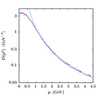
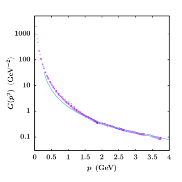
Finally, we note that for momenta larger than about $1.5$–$2.0\leavevmode\nobreak\ \text{GeV}$ both propagators are essentially perturbative. Indeed, as one can see in Fig. 3, the data are well fitted by the expression

$$f(p^{2})\,=\,c\,\log^{-13/22}(p^{2}/\Lambda^{2})\,/\,p^{2}\;,$$ (8)

for $\sqrt{p^{2}}\geq 2.0\leavevmode\nobreak\ \text{GeV}$ in the gluon case and by the expression

$$f(p^{2})\,=\,c\,\log^{-9/44}(p^{2}/\Lambda^{2})\,/\,p^{2}\;,$$ (9)

for $\sqrt{p^{2}}\geq 1.5\leavevmode\nobreak\ \text{GeV}$ in the ghost case. [Note that we have included in the fitting functions the (one-loop) anomalous dimensions (with $N_{f}=0$) for the two propagators.] In particular, in the first case we find $c=2.31\pm 0.05$ and $\Lambda=0.31\pm 0.03\leavevmode\nobreak\ \text{GeV}$ with $\chi^{2}/\mathrm{dof}=1.73$, while in the second one we obtain $c=1.71\pm 0.04$ and $\Lambda=0.43\pm 0.07\leavevmode\nobreak\ \text{GeV}$ with $\chi^{2}/\mathrm{dof}=0.54$. Thus, below we will focus the Padé analysis mostly in the IR region. We note that, although we are allowed to consider at small momenta Padé approximants $P^{M}_{N}(p^{2})$ that do not necessarily satisfy the leading $p^{-2}$ ultraviolet (UV) behavior of the propagators, the sequences that have the correct UV behavior are expected to display a faster convergence.

5 Results

We now turn to the use of the Padé approximants of Eq. (1) as fitting functions to the lattice data for gluon and ghost propagators described in Sec. 4. The central values of the parameters are obtained through the minimization of a $\chi^{2}$ function taking into account all errors and correlations (when necessary). The fit uncertainties were calculated with several different methods (Hessian matrix, Monte Carlo error propagation, $\Delta\chi^{2}$, and linear error propagation, as discussed in Sec. 3) and we always find good agreement between the results. For the final statistical errors we quote the values from the Hessian matrix. The fit quality is judged by the $\chi^{2}$ per degree of freedom (dof) and we give the associated $p$-value in each case. We limit our fits to approximants of relatively low orders (up to 10 parameters), which keeps the errors under control given the limitations imposed by the data set. Finally, when extracting pole positions, zeros, and other quantities from the rational approximants we always propagate all the errors, taking into account the correlations between the fit parameters (obtained from the Hessian matrix of the fit).

The above analysis ensures a good control of the statistical errors of our results and, as described below, it has been directly applied to the gluon-propagator data. However, when dealing with the ghost-propagator data, this procedure requires some adaptations, due to the stronger correlations present in these data. In particular, the fit quality has to be modified, considering only the diagonal elements of the covariance matrix, and the error propagation is evaluated using a linear approximation, taking into account all correlations. This is discussed in detail in Sec. 5.2 and in Appendix A.

5.1 Padé approximants to the Landau-gauge gluon propagator

For the gluon propagator we limit our fitting procedure, described above, to approximants of relatively low orders (at most 7 parameters), which keeps the errors under control, given the limitations imposed by the data set (see discussion in the previous section). As a first step, comparing fits with and without correlations between the lattice data points, we have checked explicitly that the correlations in the data sets are negligible and thus can be disregarded in the fitting procedure, in agreement with Refs. [80, 30]. Then, we performed trial fits, using different numbers of data points, and compared our results with those presented in Ref. [41]. We find that, by restricting the fits to $\sqrt{p^{2}}<1.63\leavevmode\nobreak\ \text{GeV}$ (corresponding to 100 data points) the fit quality is very good — with high $p$-values — but the obvious trade-off is that the parameters have larger errors, due to the reduced information. Conversely, by increasing the number of data points, the errors become smaller but the fit quality decreases. It turns out that by restricting the fits to $\sqrt{p^{2}}<2.4\leavevmode\nobreak\ \text{GeV}$ (corresponding to 160 data points) we obtain acceptable fits — with $p$-values of the order of a percent — while having errors on the parameters that are small in comparison to fits with fewer data points. Thus, with this choice, we restrict our analysis mostly to the IR region, which is the main focus of our study, since in this limit the propagator is not described by the perturbative behavior. Therefore, all the fits reported below are performed for $\sqrt{p^{2}}<2.4\leavevmode\nobreak\ \text{GeV}$, with 160 data points in total. In any case, we checked that the results do not show a strong dependence on this choice.

Before presenting our general results for the gluon propagator, we analyze in detail, as an example, the case of a low-order approximant. Of course, one could start with the simplest option $P_{1}^{1}(p^{2})$, but fits with Padés of the type $P_{1}^{N}(p^{2})$ lead to very bad fits, with extremely small $p$-values. Indeed, due to the trivial structure of their denominator, these Padés are forced to have a real pole, which turns out to be incompatible with a precise description of the lattice data for the gluon propagator in the IR region. Therefore, these approximants are not included in our analysis and we start our study with the Padé $P_{2}^{1}(p^{2})$, whose expression is given by

$$P_{2}^{1}(p^{2})=\dfrac{a_{0}+a_{1}\,p^{2}}{1+b_{1}\,p^{2}+b_{2}\,p^{4}}\;.$$ (10)

As already stressed above, this approximant corresponds to the function $f_{1}(p^{2})$ of Ref. [41], which arises in the context of the Gribov-Zwanziger scenario [62, 81, 3] for the description of the gluon propagator. At the same time, note that this approximant is the first in the sequence $P_{N+1}^{N}(p^{2})$, which is considered here, allowing us to analyze the data in a systematic and model-independent way. Using this Padé approximant as the fitting function to perform a $\chi^{2}$ minimization, we obtain $\chi^{2}/\mathrm{dof}=1.28$ and a $p\mathrm{-value}$ of $0.010$, which indicates an acceptable — although not impressive — fit quality. The corresponding PA’s parameters with their statistical uncertainties, as determined by the fit, are

$$a_{0} =(3.82\pm 0.02)\,\,\,\mathrm{GeV}^{-2}\;,\qquad\qquad a_{1}=(1.21\pm 0.06)\,\,\,\mathrm{GeV}^{-4}\;,$$

$$b_{1} =(1.18\pm 0.02)\,\,\,\mathrm{GeV}^{-2}\;,\qquad\qquad b_{2}=(1.65\pm 0.05)\,\,\,\mathrm{GeV}^{-4}\;,$$ (11)

with the following non-trivial correlation coefficients

$$\begin{array}[]{c|ccc}&a_{1}&b_{1}&b_{2}\\ \hline\cr a_{0}&-0.426&0.821&-0.436\\ a_{1}&-&-0.586&0.995\\ b_{1}&-&-&-0.632\end{array}\;\;.$$ (12)

We remark that some of the fit parameters are quite strongly correlated, which must be taken into account in subsequent error propagations.

Using the fit results we can now extract the poles and the zeros of this approximant, carefully propagating the uncertainties by taking into account the correlations between the fit parameters. The PA $P_{2}^{1}(p^{2})$ has a pair of complex poles located at

$$p^{2}=\left[(-0.36\pm 0.02)\pm i\,(0.690\pm 0.005)\right]\,\,\mathrm{GeV}^{2}\;,$$ (13)

and a zero on the negative real axis at

$$p^{2}=(-3.2\pm 0.2)\,\,\,\mathrm{GeV}^{2}\;.$$ (14)

We will see below that these complex poles and the zero are still present in higher-order PAs, which is a strong indication of the fact that they are genuine features of the gluon propagator in the IR and not transient artifacts.

We can also study the behavior of the propagator near $p^{2}\approx 0$ by obtaining an estimate of its Taylor-series coefficients. By writing the Taylor series of the gluon propagator around $p^{2}=0$ as

$$D(p^{2})=c_{0}+c_{1}\,p^{2}+c_{2}\,p^{4}+c_{3}\,p^{6}+c_{4}\,p^{8}+\cdots\;,$$ (15)

and by expanding the Padé given in Eq. (10) (again taking into account the correlations in the error propagation), we find the coefficients

$$c_{0} =3.82\pm 0.02\,\,\,\mathrm{GeV}^{-2}, c_{1} =-3.3\pm 0.1\,\,\,\mathrm{GeV}^{-4}, c_{2} =-2.4\pm 0.4\,\,\,\mathrm{GeV}^{-6},$$

$$c_{3} =8.3\pm 0.4\,\,\,\mathrm{GeV}^{-8}, c_{4} =-5.9\pm 0.6\,\,\,\mathrm{GeV}^{-10}, c_{5} =-7\pm 2\,\,\,\mathrm{GeV}^{-12}.$$ (16)

We can see that the first few coefficients have rather small errors, which could serve as an additional constraint to the theoretical description of the gluon propagator in the IR.

Table 1: Complex poles of the Padé approximants used as fitting functions to the Landau-gauge gluon-propagator lattice data, together with the $\chi^{2}/\mathrm{dof}$ and the p-value of the respective fits. Results from $P_{2}^{3}(p^{2})$ and $P_{3}^{3}(p^{2})$ do not enter our final values (see text).

PA	complex poles $(\mathrm{GeV}^{2})$	$\chi^{2}/\mathrm{dof}$	p-value
$P_{2}^{1}$	$(-0.36\pm 0.02)\pm i\,(0.690\pm 0.005)$	1.28	0.010
$P_{3}^{1}$	$(-0.32\pm 0.02)\pm i\,(0.65\pm 0.03)$	1.27	0.012
$P_{2}^{2}$	$(-0.32\pm 0.02)\pm i\,(0.65\pm 0.02)$	1.28	0.012
$P_{3}^{2}$	$(-0.47\pm 0.05)\pm i\,(0.66\pm 0.03)$	1.19	0.055
$P_{2}^{3}$	$(-0.27\pm 0.01)\pm i\,(0.49\pm 0.04)$	1.18	0.060
$P_{3}^{3}$	$(-0.5\pm 0.7)\pm i\,(0.07\pm 3.3)$	1.18	0.068

The results obtained using the PA $P_{2}^{1}(p^{2})$ for the complex pole, the zero, and the Taylor-series coefficients should, of course, be corroborated by the investigation of PAs of higher orders, in the same sequence as well as in other near-diagonal sequences. In Table LABEL:tab:PAspoles, we display our findings for the complex pole position extracted from PAs belonging to the sequences $P_{N}^{N}$, $P_{N}^{N+1}$, $P^{N}_{N+2}$, and $P_{N+1}^{N}$. In each case we also give the value of the $\chi^{2}/{\rm dof}$, as well as the accompanying $p$-value. All fits are reasonable from the point of view of the fit quality. The parameter errors and the errors entailed in the pole position, however, grow rapidly once the number of parameters exceeds 6. Indeed, the PAs $P^{2}_{3}(p^{2})$ and $P_{3}^{3}(p^{2})$ have parameters $a_{i}$ and $b_{i}$ with errors of the order of (or larger than) 100%, and some of the parameters are more than 99% correlated. Thus, these PAs have a number of parameters that are already at the limit of what can be done with the lattice data at hand and, therefore, we refrain from showing any results for PAs of even larger orders. Nevertheless, somewhat surprisingly, the pole position obtained with $P_{3}^{2}(p^{2})$ has acceptable (even though larger) errors, and corroborates the outcomes from the lower-order PAs. These not-so-large errors, in this case, are the result of the interplay between the large parameter errors and their strong (mostly positive) correlations, which leads to a partial cancellation of the final error in the pole position. On the contrary, in the case of $P_{3}^{3}(p^{2})$, the large parameter errors do translate into very large errors for the pole position, as shown in the final row of Table LABEL:tab:PAspoles. Because of these huge errors and correlations, we do not use $P_{3}^{3}(p^{2})$ — or $P_{2}^{3}(p^{2})$, as discussed below — for our final values.

Figure 4: Comparison of the Padé approximants used to determine the final results and the lattice data. The shaded region — corresponding to $p=\sqrt{p^{2}}\geq 2.4\leavevmode\nobreak\ \text{GeV}$ — is not included in the fits.

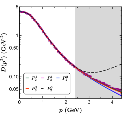
The results of the fits of Table LABEL:tab:PAspoles are also shown, compared to the lattice data, in Fig. 4. In this figure one can see the extrapolation of the PA results beyond the fit region. In all cases, with the exception of $P^{3}_{2}(p^{2})$, the PAs follow the expected behavior, at least qualitatively. Note that the bad UV behavior of $P^{3}_{2}(p^{2})$ can be understood, since this approximant goes as $a_{4}p^{2}$ for large $p^{2}$, with a positive — although statistically compatible with zero — coefficient $a_{4}=0.05(20)\,{\rm GeV}^{-10}$. Clearly, the known fall-off of the propagator in the perturbative regime disfavors the sequences $P_{N}^{N+k}(p^{2})$, with $k>0$, for a precise description of the propagator in the full energy range. It is customary to exclude PAs with the wrong high-energy behavior from analyses of this type, since this will necessarily delay the convergence of the approximants [46]. Due to this behavior of $P^{3}_{2}(p^{2})$ at higher energies, we do not include it in our final estimate for the complex pole position, since this inclusion leads to an artificial increase of the systematic error.

(a)

(b)

Figure 5: Padé approximants used to determine the final results. In (a) we have the poles of each PA and in (b) the zeros. In both cases, we show our final prediction in black. Note that the Padés $P_{2}^{1}$ and $P_{3}^{2}$ belong to the same sequence $P_{N+1}^{N}$. Also note that in this plot we added in quadrature the two types of errors.

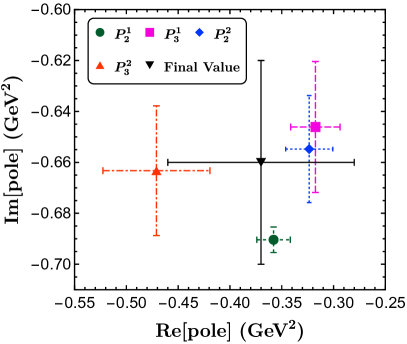
The results of Table LABEL:tab:PAspoles show in all the PAs a consistent pair of complex poles that pass the consistency checks discussed above. We can then extract our final value for the pole position using the results of $P^{1}_{2}$, $P^{1}_{3}$, $P_{2}^{2}$, and $P^{2}_{3}$. We quote as our final central value the (arithmetic) average of the results obtained from these four PAs. Because the different results are based on the same data set and are therefore obviously correlated, it does not make sense to reduce the uncertainty through a weighted-average procedure and — to remain conservative — we quote, as our final statistical uncertainty, the largest one from the individual PAs. Finally, it is crucial to include a systematic uncertainty due to the method we employ. We estimate this uncertainty dividing by $2$ the maximum spread between results from two different PAs. This leads to the following value for the position of the complex pole

$$p_{\rm pole}^{2}=[(-0.37\pm 0.05_{\rm stat} \pm 0.08_{\rm sys})\,\,\pm$$

$$\pm\,\,i\,(0.66\pm 0.03_{\rm stat}\pm 0.02_{\rm sys})]\,\,\mathrm{GeV}^{2}\;,$$ (17)

where “stat” and “sys” denote the statistical uncertainty and systematic error from the PA method, respectively. This shows very clearly that the PAs favor the existence of a pair of complex poles, with an imaginary part incompatible with zero. The results for the pole position in the complex plane are summarized in Fig. 5a.

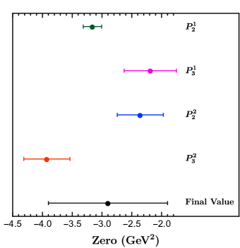
Another salient feature of all the PAs shown in Table LABEL:tab:PAspoles is the presence of a zero along the real axis. This indicates that this zero is physical and we can estimate its position using the same procedure described above for the pair of complex poles. This leads to

$$p_{\rm zero}^{2}=(-2.9\pm 0.4_{\rm stat}\pm 0.9_{\rm sys})\,\,\mathrm{GeV}^{2}\;.$$ (18)

The results for the zero of the PAs are shown in Fig. 5b.

Table 2: Values for the first five Taylor coefficients $c_{n}$ of the gluon propagator predicted by the Padé approximants (with statistical errors). Shaded results have uncertainties larger than 25% and do not enter our final values.

	$c_{0}$ ($\mathrm{GeV}^{-2}$)	$c_{1}$ ($\mathrm{GeV}^{-4}$)	$c_{2}$ ($\mathrm{GeV}^{-6}$)	$c_{3}$ ($\mathrm{GeV}^{-8}$)	$c_{4}$ ($\mathrm{GeV}^{-10}$)
$P_{2}^{1}$	$3.82\pm 0.02$	$-3.3\pm 0.1$	$-2.4\pm 0.4$	$8.3\pm 0.4$	$-5.9\pm 0.6$
$P_{3}^{1}$	$3.81\pm 0.02$	$-3.0\pm 0.2$	$-3.7\pm 0.9$	$10\pm 1$	$-5.5\pm 0.9$
$P_{2}^{2}$	$3.81\pm 0.02$	$-3.1\pm 0.2$	$-3.5\pm 0.8$	$10\pm 1$	$-5.6\pm 0.8$
$P_{2}^{3}$	$3.78\pm 0.02$	$-2.1\pm 0.4$	$-9\pm 2$	$23\pm 6$	$-11\pm 4$
$P_{3}^{2}$	$3.74\pm 0.03$	$1\pm 3$	$-86\pm 109$	$1257\pm 2653$	$-18149\pm 54434$
$P_{3}^{3}$	$3.76\pm 0.03$	$-0.8\pm 1.5$	$-25\pm 24$	$119\pm 207$	$-397\pm 1230$

Table 3: Final estimates for the Taylor-series coefficients of the gluon propagator. In each line, the first uncertainty is statistical while the second is systematic, obtained from the spread of values from the different PAs.

$c_{0}$	$(3.79\pm 0.03_{\rm stat}\pm 0.04_{\rm sys})$ $\mathrm{GeV}^{-2}$
$c_{1}$	$(-2.9\pm 0.4_{\rm stat}\pm 0.6_{\rm sys})$ $\mathrm{GeV}^{-4}$
$c_{2}$	$(-5\pm 2_{\rm stat}\pm 3_{\rm sys})$ $\mathrm{GeV}^{-6}$
$c_{3}$	$(9.4\pm 1.0_{\rm stat}\pm 0.9_{\rm sys})$ $\mathrm{GeV}^{-8}$
$c_{4}$	$(-5.7\pm 0.9_{\rm stat}\pm 0.2_{\rm sys})$ $\mathrm{GeV}^{-10}$

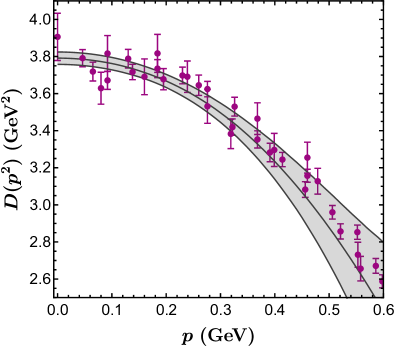
We now turn to the determination of the Taylor coefficients for the expansion of the Landau-gauge gluon propagator around $p^{2}=0$. The results for the first five Taylor coefficients obtained with the PAs are shown in Table LABEL:tab:PAscoeffs. In all cases, the constant $c_{0}$ is very well determined. The statistical uncertainties grow with the order of the coefficients $c_{n}$, as well as with the order of the PAs. We include in our final determination of the coefficients $c_{n}$ the results with relative statistical uncertainty smaller than 25%, as shown in Table LABEL:tab:PAscoeffs. We follow again the procedure outlined above, i.e. we obtain the final Taylor coefficients from the average of the central values. Also, the final statistical uncertainty is the largest among the individual PAs that contribute to the final value, and the systematic uncertainty is half of the maximum spread between the individual determinations. The final results are shown in Table LABEL:tab:finalcoeff. The final values for the $c_{n}$ coefficients, up to order four, are then used to plot the propagator obtained from the Taylor expansion, Eq. (15), compared with the data points. This result is shown in Fig. 6 and represents a model-independent constraint on the behavior of the lattice gluon propagator for $p=\sqrt{p^{2}}<0.6\leavevmode\nobreak\ \text{GeV}$. The error band of Fig. 6 is obtained from a Monte Carlo error propagation by randomly generating 5000 values for each of the Taylor coefficients, assuming that they follow a uniform distribution, since the errors are dominated by the systematic component. The central value is then the median of the 5000 values obtained for the Taylor series and the uncertainty band represents the 68% confidence level interval.

Figure 6: Landau-gauge gluon-propagator Taylor series (gray) up to fifth order, from the results of Table LABEL:tab:finalcoeff. The uncertainty band is the 68% confidence level, assuming a uniform distribution for the Taylor-series coefficients. The lattice data from Ref. [39, 9, 40] are shown in purple.

5.2 Padé approximants to the Landau-gauge ghost propagator

We now turn to the analysis of the Landau-gauge ghost propagator. The method is the same as in the previous section, which allows for a streamlined discussion of the results. The main difference with respect to the gluon-propagator case concerns the correlations in the data sets from different configurations. Indeed, for the ghost-propagator data, these correlations are substantial. As a matter of fact, the correlation matrix has several non-diagonal entries with values as large as 0.75. Fits to strongly correlated data are known to be problematic, since they can lead to biased [82], or simply unreliable, results [83]. In particular, in strongly correlated data, the correlation (or covariance) matrix has very small eigenvalues. As a consequence, its numerical inversion is problematic and its inverse contains very large numbers, which contribute with large and quasi-random fluctuations in the $\chi^{2}$ value, spoiling the fit results. In this situation, one often resorts to fits where the off-diagonal correlations do not enter the fit quality, simply by considering a diagonal covariance matrix. We refer to fits of this type as “diagonal fits” [83] and, in this case, we denote the fit quality by ${Q}^{2}$, instead of the usual $\chi^{2}$. Thus, for the analysis of the ghost propagator, we will perform diagonal fits. We will, however, include all correlations in the error propagation, following the procedure of Ref. [83], which is described in Appendix A. This method allows for unbiased fits with reliable errors. On the other hand, since we use a diagonal covariance matrix, we do not have a strict statistical interpretation for the measure of the fit quality given by $Q^{2}/{\rm dof}$. Therefore, we cannot judge the fit quality in absolute terms, but only by comparison with other similar fits. For this reason, we do not quote $p$-values in association with $Q^{2}$-type fits.

Table 4: Location of the pole, on the negative real axis of $p^{2}$, from the partial Padé approximants — used as fitting functions to the Landau-gauge ghost-propagator lattice data — together with the corresponding $Q^{2}/\mathrm{dof}$ value. Results from $\mathbb{P}_{4}^{4}(p^{2})$ and $\mathbb{P}_{5}^{4}(p^{2})$ do not enter our final values, due to their large errors.

PPA	pole $(\mathrm{GeV}^{2})$	$Q^{2}/\mathrm{dof}$
$\mathbb{P}_{1}^{1}$	$-0.30\pm 0.05$	0.65
$\mathbb{P}_{2}^{1}$	$-0.33\pm 0.05$	0.60
$\mathbb{P}_{1}^{2}$	$-0.33\pm 0.05$	0.60
$\mathbb{P}_{2}^{2}$	$-0.32\pm 0.05$	0.59
$\mathbb{P}_{3}^{1}$	$-0.27\pm 0.04$	0.54
$\mathbb{P}_{3}^{3}$	$-0.29\pm 0.04$	0.32
$\mathbb{P}_{4}^{3}$	$-0.28\pm 0.03$	0.32
$\mathbb{P}_{5}^{3}$	$-0.24\pm 0.05$	0.28
$\mathbb{P}_{4}^{4}$	$-0.1\pm 0.1$	0.27
$\mathbb{P}_{5}^{4}$	$-0.16\pm 0.08$	0.25

We start again our analysis with the Padé approximant $P_{2}^{1}(p^{2})$, since the PAs with fewer parameters led to very bad fits. All fit parameters in this case turn out to be of the order of $10^{10}$, which can be seen as a manifestation of the existence of a pole very close to the origin, namely at $p^{2}\approx-1.2\times 10^{-10}\leavevmode\nobreak\ \text{GeV}^{2}$. The appearance of a pole at $p^{2}\approx 0$ and of very large fit parameters occurs for higher-order PAs as well. This is a clear indication that this pole at the origin is a physical one and thus must be explicitly enforced in the structure of the PAs, in order to obtain fit parameters of a natural size. This can be done using the so-called partial Padé approximants (PPAs) [84] that we define as

$$\mathbb{P}^{M}_{N,k}(p^{2})=\frac{Q_{M}(p^{2})}{R_{N}(p^{2})\,T_{k}(p^{2})}\;,$$ (19)

where the polynomials $Q_{M}(p^{2})$ and $R_{N}(p^{2})$ are the same as before and in $T_{k}(p^{2})$ we impose the existence of $k$ poles. In particular, here, we use simply $k=1$ with

$$T_{1}(p^{2})=p^{2}\;,$$ (20)

which imposes the pole at $p^{2}=0$. In order to simplify the notation, we denote these PPAs $\mathbb{P}^{M}_{N,1}(p^{2})$ just as $\mathbb{P}^{M}_{N}(p^{2})$. Let us note that an alternate procedure, which leads to the same results, is to fit the data for $p^{2}\,G(p^{2})$, effectively removing the singularity at the origin.

As a preliminary step, we have again investigated fits using different fit windows. The results we report below are for fits restricted to the interval $\sqrt{p^{2}}\leq 3.12\leavevmode\nobreak\ \text{GeV}$, which contains 220 data points and enters the region that is well described by the perturbative prediction, as shown in Fig. 3b. (We stress, however, that our main results are largely independent of the chosen fit window.) The primary reason for our final decision is that this choice avoids, in some of the PPAs, the appearance of Froissart doublets located in the region where lattice data are available. We recall that these doublets are expected to appear, in a transient form, in some of the approximants and that they are harmless, as long as we use the PPAs away from these singularities. However, they can spoil the extrapolation of the fit results beyond the fit window.

(a)

(b)

Figure 7: Location of the (a) pole and (b) zero from the partial Padé approximants, fitted to the Landau-gauge ghost-propagator lattice data. Results from approximants belonging to the same sequence are shown in the same color [blue for $\mathbb{P}^{N}_{N}(p^{2})$, orange for $\mathbb{P}^{N}_{N+1}(p^{2})$ and pink for $\mathbb{P}^{N}_{N+2}(p^{2})$]. Our final values are shown in black at the bottom of each plot. As before, in this plot we add in quadrature the statistical and systematic errors. The pole followed by a zero points towards the presence of a branch cut along the negative real axis of $p^{2}$. (See discussion in the text.)

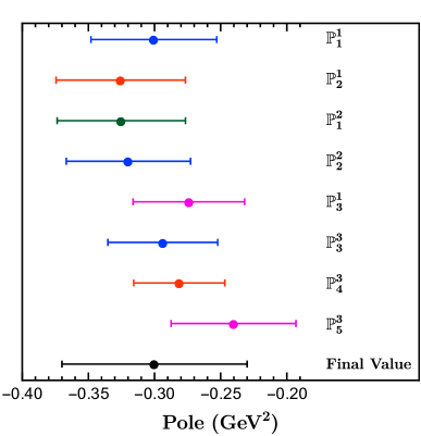
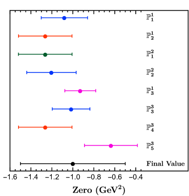
We employed partial Padés, belonging to the sequences $\mathbb{P}_{N}^{N}$, $\mathbb{P}_{N}^{N+1}$, $\mathbb{P}_{N+1}^{N}$, and $\mathbb{P}_{N+2}^{N}$, to fit the ghost-propagator data. Here, the approximants that play a special role are those belonging to the sequence $\mathbb{P}^{N}_{N}(p^{2})$, since they have a built-in $1/p^{2}$ behavior at large $p^{2}$, which should lead to a faster convergence. We note that a salient feature of all approximants is the appearance of a pole located on the negative real axis of $p^{2}$. These results are shown in Table LABEL:tab:PAsghostpoles, together with the associated values of $Q^{2}/\mathrm{dof}$ from each fit. Clearly, the position of this pole on the negative real axis is remarkably stable, which strongly suggests that it has a physical nature. At the same time, approximants with more than 8 parameters, such as $\mathbb{P}_{4}^{4}(p^{2})$ and $\mathbb{P}_{5}^{4}(p^{2})$ in Table LABEL:tab:PAsghostpoles, have strongly correlated fit parameters, of the order of 99%, and fit-parameter errors larger than 100%. Since such large uncertainties lead to predictions with substantial errors, these PAs will not enter our final estimates. We stress that a similar behavior has already been observed for the PAs with more than 6 parameters in the analysis of the gluon-propagator data.

Figure 8: Plot of the partial Padé approximants, used to determine our final results, and of the lattice data for the Landau-gauge ghost propagator. The shaded region – corresponding to $p=\sqrt{p^{2}}>3.12\leavevmode\nobreak\ \text{GeV}$ — is not included in the fits.

From the results shown in Table LABEL:tab:PAsghostpoles, we can obtain a final estimate for the location of the pole predicted by the PPAs, by employing the same procedure used for the gluon-propagator analysis: the central value is the mean of all the results obtained from the PPAs, the statistical uncertainty is the largest error from a single Padé, and the systematic uncertainty is half the maximum difference of two PPA results. Thus, our final estimate for the pole position on the real axis is

$$p^{2}_{\mathrm{pole}}=(-0.30\pm 0.05_{\mathrm{stat}}\pm 0.05_{\mathrm{sys}})\,\,\mathrm{GeV}^{2}\;.$$ (21)

The results for the pole position of individual PPAs, as well as our final result, are summarized in Fig. 7a. At the same time, the fitted approximants also suggest the existence of a zero on the negative real axis of $p^{2}$, which, by applying the same method as before, is predicted to be at

$$p^{2}_{\mathrm{zero}}=(-1.0\pm 0.3_{\mathrm{stat}}\pm 0.4_{\mathrm{sys}})\,\,\mathrm{GeV}^{2}\;.$$ (22)

The location of the zeros from the different PPAs are shown in Fig. 7b (together with our final estimate). It is important to remark that the existence of a pole followed by a zero along the negative real axis may be, in fact, the manifestation of a branch cut — a possibility that we discuss further below.

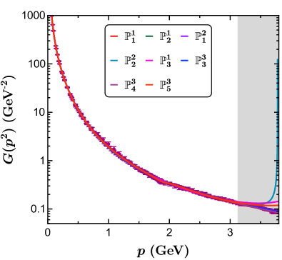
The results from the PPAs considered in Table LABEL:tab:PAsghostpoles and in Fig. 7 are exhibited in Fig. 8, compared to the lattice data for $G(p^{2})$; the shaded area indicates the region not included in the fit window. We note that the approximant $\mathbb{P}_{2}^{2}(p^{2})$ has a Froissart doublet, i.e. a pole partially cancelled by a nearby zero, on the positive real axis, but located outside the fit region. As said above, this is, typically, a transient artifact of the rational approximants. Indeed, the doublet disappears when the order of the PPA is increased and it is already not present in the approximant $\mathbb{P}^{3}_{3}(p^{2})$.

Table 5: Values for the first five Taylor coefficients $r_{n}$ of the ghost propagator predicted by the partial Padé approximants (with statistical errors). Shaded results have uncertainties larger than 45% and do not enter our final values.

	$r_{0}$	$r_{1}$ ($\mathrm{GeV}^{-2}$)	$r_{2}$ ($\mathrm{GeV}^{-4}$)	$r_{3}$ ($\mathrm{GeV}^{-6}$)	$r_{4}$ ($\mathrm{GeV}^{-8}$)
$\mathbb{P}_{1}^{1}$	$4.17\pm 0.01$	$-10\pm 1$	$33\pm 10$	$-111\pm 51$	$369\pm 228$
$\mathbb{P}_{2}^{1}$	$4.17\pm 0.01$	$-9\pm 1$	$29\pm 8$	$-89\pm 39$	$275\pm 161$
$\mathbb{P}_{1}^{2}$	$4.17\pm 0.01$	$-9\pm 1$	$29\pm 8$	$-90\pm 39$	$276\pm 161$
$\mathbb{P}_{2}^{2}$	$4.17\pm 0.01$	$-10\pm 1$	$30\pm 8$	$-94\pm 40$	$293\pm 168$
$\mathbb{P}_{3}^{1}$	$4.17\pm 0.01$	$-10\pm 1$	$38\pm 10$	$-138\pm 58$	$503\pm 288$
$\mathbb{P}_{3}^{3}$	$4.17\pm 0.01$	$-10\pm 1$	$34\pm 9$	$-117\pm 48$	$398\pm 221$
$\mathbb{P}_{4}^{3}$	$4.17\pm 0.01$	$-10\pm 1$	$37\pm 9$	$-131\pm 47$	$466\pm 225$

Table 6: Final estimates for the Taylor-series coefficients of the ghost propagator. In each line, the first uncertainty is statistical while the second is systematic, obtained from the spread of values from the different PPAs.

$r_{0}$	$4.17\pm 0.01_{\mathrm{stat}}$
$r_{1}$	$-9.7\pm 1.0_{\mathrm{stat}}\pm 0.5_{\mathrm{sys}}$ $\mathrm{GeV}^{-2}$
$r_{2}$	$33\pm 10_{\mathrm{stat}}\pm 5_{\mathrm{sys}}$ $\mathrm{GeV}^{-4}$
$r_{3}$	$-110\pm 58_{\mathrm{stat}}\pm 25_{\mathrm{sys}}$ $\mathrm{GeV}^{-4}$

As recalled above, the pattern of a pole (at about $p^{2}=-0.3\leavevmode\nobreak\ \text{GeV}^{2}$) followed by a zero (at about $p^{2}=-1.0\leavevmode\nobreak\ \text{GeV}^{2}$) suggests that this may be the manifestation of a branch cut in $G(p^{2})$. Indeed, as described in Sec. 3, PAs mimic the existence of a cut by accumulating a series of poles interleaved with zeros along the cut. On the other hand, this is clearly observed only in very-high-order Padés, since Froissart doublets may also appear in the process, as seen in Fig. 1a. At the same time, if we go to higher orders (i.e., Padés with more than 8 parameters), pole positions and zeros have — as already noted above — a very large uncertainty, of the order of 100%, which obscures the results. Their central values, however, do show a clear pattern of poles interleaved with zeros. For example, in $\mathbb{P}^{4}_{4}(p^{2})$ we have (apart from two new Froissart doublets) a pole at $-0.10\leavevmode\nobreak\ \text{GeV}^{2}$, followed by a zero at $-0.11\leavevmode\nobreak\ \text{GeV}^{2}$, and again a pole at $-0.43\leavevmode\nobreak\ \text{GeV}^{2}$, and finally a zero at $-1.3\leavevmode\nobreak\ \text{GeV}^{2}$. Similarly, in $\mathbb{P}^{4}_{5}(p^{2})$ one finds poles at $-0.16\leavevmode\nobreak\ \text{GeV}^{2}$ and $-0.84\leavevmode\nobreak\ \text{GeV}^{2}$, which are interleaved with two zeros, at $-0.25\leavevmode\nobreak\ \text{GeV}^{2}$ and $-2.4\leavevmode\nobreak\ \text{GeV}^{2}$. This pattern corroborates the idea that the pole and the zero we find in lower-order approximants may be the first manifestation of a branch cut, along the negative real axis of $p^{2}$. We will investigate this possibility further in the next section, using the so-called D-Log Padé approximants.

Finally, as we did for the gluon propagator, we can extract the Taylor-series coefficients for $p^{2}\,G(p^{2})$ around $p^{2}=0$, which can be written as

$$p^{2}\,G(p^{2})=r_{0}+r_{1}\,p^{2}+r_{2}\,p^{4}+r_{3}\,p^{6}+r_{4}\,p^{8}+\cdots\;.$$ (23)

The first five coefficients $r_{n}$ predicted by the PPAs are shown in Table 5. One can notice that the determination of the coefficient $r_{0}$ is very consistent for the various Padés used and that the uncertainties increase considerably for higher orders. In order to obtain our final Taylor coefficients, we will employ all results with errors smaller than 45%, as indicated in Table 5. Our final estimates for the coefficients $r_{n}$ up to third order are displayed in Table 6, where the systematic and statistical errors are calculated using the same procedure as before. Assuming these values, we compare the Taylor-expanded result for $p^{2}\,G(p^{2})$ with the lattice data in Fig. 9. We see that our findings, which are model-independent, reproduce well the behavior of the ghost-propagator data up to $p=\sqrt{p^{2}}=0.5\leavevmode\nobreak\ \mathrm{GeV}$.

Figure 9: Landau-gauge ghost-propagator Taylor series (gray) up to third order, using the results of Table 6. The uncertainty band is the 68% confidence level, assuming a uniform distribution for the Taylor-series coefficients. The lattice data are shown in purple.

5.2.1 D-Log Padé approximants

The results of the previous section, obtained with PPAs as fitting functions to the Landau-gauge ghost-propagator data set, are robust and show a pole and a zero on the negative real axis of $p^{2}$. However, as already stressed above, since the pole is accompanied with a zero, one cannot exclude that this is the manifestation of a branch cut along the negative real axis. This possibility is, in fact, corroborated by the investigation of higher-order approximants, which do show a pattern of poles interleaved with zeros (albeit with very large uncertainties in their positions). We stress that, working only with the usual PAs (and PPAs), it is quite difficult — given the limitations imposed by the data — to establish whether the pole is mimicking a branch point or is, in fact, a physical pole. In this section, we perform a first exploration of a different strategy to extract information about a possible cut in the ghost propagator, namely we use the so-called D-Log Padé approximants [44] (see also [53, 54] for recent applications). The main goal of this explorative analysis is to discuss the prospects, the advantages, and the limitations of D-Log PAs when applied to the Landau-gauge ghost-propagator data.

The idea behind D-Log PAs is to manipulate a function having a cut in the complex plane into a form that can be better approximated by PAs, and later unfold the procedure. To this end, let us suppose we are interested in the following function

$$f(z)=A(z)\,\dfrac{1}{(\mu-z)^{\gamma}}+B(z)\;,$$ (24)

where $A(z)$ and $B(z)$ have a simple structure and are analytic at $z=\mu$, and $\gamma$ is not necessarily an integer — so that $f(z)$ can have a cut with branch point $z=\mu$. Instead of working directly with $f(z)$, we use a related function $F(z)$ given by

$$F(z)=\dfrac{\mathrm{d}}{\mathrm{d}z}\ln{f(z)}\approx\dfrac{\gamma}{(\mu-z)}\;,$$ (25)

where on the right-hand side we assume $z\approx\mu$. Clearly, the function $F(z)$ is, in this case, meromorphic and the usual convergence theorems apply. We stress that the exponent of the cut is now the residue of the simple pole of $F(z)$, which can, in principle, be determined in an unbiased way using Padé approximants — denoted in this context by $\bar{P}^{M}_{N}(z)$ — to $F(z)$. Then, by unfolding this procedure, the original function $f(z)$ is approximated by a non-rational function, the so-called D-Log Padé approximant, given by

$$\mathrm{Dlog}_{N}^{M}(z)=f_{\mathrm{norm}}(0)\,\exp{\left\{\int\mathrm{d}z\,\,\bar{P}_{N}^{M}(z)\right\}}\;,$$ (26)

where the constant $f_{\mathrm{norm}}(0)$ has to be adjusted to reproduce the function $f(z)$ at zero, since the constant value $f(0)$ — in the Taylor expansion of $f(z)$ — is lost due to the derivative in Eq. (25).

In view of the fact that in this work we use the PAs as fitting functions to lattice data, the application of D-Log PAs to our problem requires some additional steps, in comparison with the usual PAs. Indeed, we need (lattice) data for the function $F(p^{2})$, i.e., the derivative of the logarithm of the ghost propagator $G(p^{2})$. Clearly, these data for $F(p^{2})$ can be obtained from the propagator data, by first evaluating the logarithm and, then, by taking the numerical derivative, using finite differences. However, the application of the standard formulas for the derivative requires equally-spaced data points, a property that is not satisfied by lattice data for the ghost propagator. Thus, in order to circumvent this problem, we need first to interpolate between the data points, as a means to generate a new set of data on a uniform grid. We do this using a linear interpolation, which should be sufficient for our purposes. More specifically, after taking the logarithm of the central values of the ghost-propagator data, we interpolate them and generate equally-spaced data points, with a separation of $\Delta p^{2}=0.035\leavevmode\nobreak\ \text{GeV}^{2}$. We also propagate the errors accordingly. One should note, however, that the linear interpolation introduces correlations between some of the new data points, since they may share information of the original ghost-propagator data. We calculate these correlations using standard methods [85, 86] and take them into account carefully, in all of the subsequent results. Next, the derivative at the $i$-th point of this uniform grid, $p_{i}$, can be calculated using, for example, the usual first-order formula

$$f^{\prime}_{(1)}(p^{2}_{i})\approx\dfrac{f(p^{2}_{i+1})-f(p^{2}_{i-1})}{2\,\Delta p^{2}}\;.$$ (27)

This procedure introduces, in principle, another source of correlations in the data, since the derivative obtained at nearby points may share information from the same underlying data point. This problem can be circumvented exactly by skipping the appropriate number of points, in such a way that each derivative depends on different entries of the original data set. (For example, in the case of the above first-order formula, this is achieved when the derivative is evaluated at every third point.) Another possibility, which we will use here, is to compute the first-order derivative at every second point, calculating all the correlations involved in the process, which again can be done in a rather straightforward manner. The advantage of this procedure is that the final data set contains enough points, while keeping the correlations relatively mild. (On the other hand, when computing the derivative at every point $p_{i}^{2}$, the correlations become too strong to allow for a meaningful fit.) We have also considered higher-order numerical derivatives. The number of data points, however, decreases rapidly when the order is larger than two (if one wants to reduce correlations in the data by skipping some of the points) and, for this reason, we will only consider below first-order derivatives.

As a check, we also did the same analysis described above using the bootstrap method with 5000 samples (and verified that results do not change when using 2500 samples). In all cases we find very good agreement between the data sets produced by the two analyses. In Fig. 10a, we show the results for the derivative of the logarithm of the ghost-propagator data, evaluated numerically at every second point, computing all the ensuing correlations to the data. It is evident that the uncertainties in the final data set are rather large — of the order of 100% in some cases — with significant statistical fluctuations (as one could expect). We, nevertheless, carry on with our analysis in order to understand the applicability and the limitations of the D-Log method for the data set considered here.

(a)

(b)

Figure 10: (a) First-order numerical derivative of the logarithm of the ghost-propagator data together with the Padés $\bar{P}_{M}^{N}(p^{2})$ used to build the D-Log PAs. (b) The lattice data for the ghost propagator and the D-Log Padé approximants built from the first-order numerical derivative of the logarithm of the data. The shaded region — corresponding to $p=\sqrt{p^{2}}>2.0\leavevmode\nobreak\ \text{GeV}$ — is excluded from the fit.

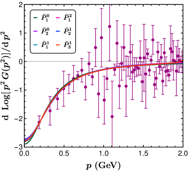
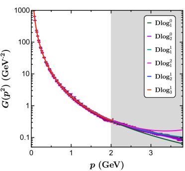
We first perform the minimization to the (generated) data set, using the PAs $\bar{P}_{N}^{M}(p^{2})$ as fitting functions. The result is shown in Fig. 10a. We again use diagonal fits, i.e., as said above, we consider in the fit quality only the diagonal elements of the covariance matrix. In this case, for the fit, we select data in the interval $p\leq 2.0\leavevmode\nobreak\ \text{GeV}$, since at larger momenta the errors and fluctuations are very large. Moreover, as clearly seen from Fig. 10a, the data at $p^{2}=2.0\leavevmode\nobreak\ \text{GeV}$ are already described by the perturbative $1/p^{2}$ behavior. After the minimization, Eq. (26) is employed to build the D-Log Padés to the ghost-propagator data. We performed fits using the D-Log sequences $\mathrm{Dlog}_{N+1}^{N}$, $\mathrm{Dlog}_{N+2}^{N}$, $\mathrm{Dlog}_{N}^{N}$ and $\mathrm{Dlog}_{N}^{N+1}$. As before, the maximum value of $N$ that can be considered is limited by the quality of the fitted data. In particular, in this case, the maximum number of parameters that lead to meaningful results is only 5, which is a consequence of the large errors and fluctuations of the data set. We find that these approximants have a branch cut of the form

$$\frac{1}{(p_{c}-p^{2})^{\gamma}}\;.$$ (28)

The branch point $p_{c}$ and the multiplicity $\gamma$ of the cut obtained from different D-Log approximants are reported in Table LABEL:tab:Dlogcutghost, together with the corresponding $Q^{2}/\mathrm{dof}$ value. One can observe that the approximants that pass all reliability tests have indeed a cut on the negative real axis, with a branch point not too far from the pole at $-0.30\leavevmode\nobreak\ \text{GeV}^{2}$, determined in the previous section. Our final value for the branch-point position is

$$p_{c}=(-0.12\pm 0.08_{\rm stat}\pm 0.02_{\rm sys})\leavevmode\nobreak\ \mathrm{GeV}^{2}\;.$$ (29)

One should stress, however, that our systematic uncertainty for $p_{c}$ may be underestimated, since the evaluation of the numerical derivative inevitably introduces an additional source of error. At the same time, the exponent $\gamma$ is clearly not compatible with one, which reinforces that the function has indeed a cut (in the negative real axis) and not a pole. Our results for the D-Log Padés, together with the original lattice data, are shown in Fig. 10b, where it is possible to observe a reasonably good agreement, even beyond the fit region.

Table 7: Branch point $p_{c}$ and the multiplicity $\gamma$, alongside the corresponding $Q^{2}/\mathrm{dof}$ value, from fits of D-Log Padé approximants to the Landau-gauge ghost-propagator lattice data.

D-Log PA	$p_{c}$ $(\mathrm{GeV}^{2})$	$\gamma$	$Q^{2}/\mathrm{dof}$
$\mathrm{Dlog}_{1}^{0}$	$-0.11\pm 0.03$	$0.31\pm 0.05$	0.81
$\mathrm{Dlog}_{2}^{0}$	$-0.14\pm 0.07$	$0.4\pm 0.2$	0.81
$\mathrm{Dlog}_{1}^{1}$	$-0.13\pm 0.05$	$0.4\pm 0.1$	0.81
$\mathrm{Dlog}_{1}^{2}$	$-0.12\pm 0.09$	$0.3\pm 0.2$	0.83
$\mathrm{Dlog}_{2}^{1}$	$-0.12\pm 0.04$	$0.3\pm 0.2$	0.83
$\mathrm{Dlog}_{3}^{1}$	$-0.12\pm 0.08$	$0.3\pm 0.2$	0.85

Figure 11: Comparison of the largest (real and nonzero) pole position from four partial Padés sequences with the branch point position obtained form the D-Log approximants, Eq. (29), shown as the gray band. At higher-orders the position of the first pole tends to approach the D-Log branch point, indicating that the PPAs are mimicking the cut. We note that the uncertainty on the gray band may be underestimated, since the application of the D-Log Padés requires the calculation of numerical derivatives from the original data set.

Let us now compare the results from the D-Log approximants with the results from the PPAs, described in the previous section. It is evident that the analysis using D-Log approximants does corroborate the existence of a branch cut on the negative real axis of $p^{2}$. Then, if the cut is indeed present, one would expect that the pole — found with the PPAs — should indicate the position of the branch point. As a matter of fact, the final results we obtain for $p_{c}$ and for the pole extracted from the PPAs [see Eqs. (29) and (21)] are compatible within $1.7\sigma$. Furthermore, we observe that, for higher-order PPAs, the position of the pole tends to larger values, i.e. to $-0.10\leavevmode\nobreak\ \text{GeV}^{2}$ and $-0.16\leavevmode\nobreak\ \text{GeV}^{2}$ respectively when considering $P^{4}_{4}(p^{2})$ and $P^{4}_{5}(p^{2})$, thus approaching the value of $p_{c}$ from the D-Log approximants, although with larger errors. This can be clearly seen in Fig. 11, where we compare $p_{c}$ from Eqs. (29) with the largest (nonzero) pole positions from different PPA sequences, with up to 10 parameters. It is evident that higher-order PPAs show a pole position in better agreement with the location of $p_{c}$ obtained from the D-Log approximants. This may indicate a possible convergence between the two methods.

In conclusion, the results of this section support, apart from the pole at $p^{2}=0$, the existence of a branch cut along negative values of $p^{2}$. Our best estimator for the branch point $p_{c}$ is obtained from the D-Log approximants, and this value is in reasonably good agreement with the results from the PPAs.

6 Conclusions

In this work we have used rational approximants in order to study the analytic structure of the IR Landau-gauge gluon and ghost propagators from a model-independent point of view. With this method, we do not rely on any specific theoretical description of the propagators in the IR. Instead, the main analytic features are obtained from a systematic use of Padé approximants (and also of partial Padé and D-Log Padé approximants) as fitting functions to the lattice data for the $SU(2)$ gluon and ghost propagators. A closely related work, applying Padé approximants to the $SU(3)$ propagators, may be found in Refs. [37, 38]. The results we present here have more robust uncertainties, since we have performed, in all cases, a careful error propagation, including all correlations in the data set as well as in the fit parameters. Apart from the statistical error, we have also estimated a theoretical systematic error, inherent to the method. Another important difference with respect to Refs. [37, 38] is that we have exploited variants of the usual Padé approximants, namely the partial Padés and the D-Log Padés, which were particularly useful in the study of the ghost propagator.

In the case of the gluon propagator, the Padé approximants show distinct evidence for a pair of complex poles located at

$$p^{2}=[(-0.37\pm 0.09)\pm i\,(0.66\pm 0.04)]\,\,\mathrm{GeV}^{2}\;,$$ (30)

where we added in quadrature the statistical and systematic errors of Eq. (5.1). This result is of course in good agreement with the analysis presented in Ref. [41] (see their Table IV) for the same set of lattice data. It is also remarkable that the pole position turns out very similar to those found in the $SU(3)$ gluon propagator, namely $p^{2}=-0.28(6)\pm i\,0.4(1)\leavevmode\nobreak\ \text{GeV}^{2}$ or $p^{2}=-0.19(4)\pm i\,0.4(1)\leavevmode\nobreak\ \text{GeV}^{2}$ — depending on the method used in the analysis of Ref. [37] — and $p^{2}=-0.30(7)\pm i\,0.49(3)\leavevmode\nobreak\ \text{GeV}^{2}$ from Ref. [32]. At the same time, we find evidence for a zero in the gluon propagator, located at $p^{2}_{\rm zero}=(-2.9\pm 1.0)\leavevmode\nobreak\ \text{GeV}^{2}$.

As for the ghost propagator, the analysis with PAs reveals that the approximants require a pole at the origin. This input has, therefore, been used to build the so-called partial Padé approximants, which provide evidence for a pole — along the negative real axis — followed by a zero. At the same time, higher-order PPAs also show additional intercalated poles and zeros. As stressed in the text, this result is an indication that the approximants may be mimicking a branch cut of the function by accumulating poles (and zeros) along the cut [44]. In order to test this hypothesis, we considered in Sec. 5.2.1 the so-called D-Log Padé approximants, which are particularly useful to study functions with a branch cut. Indeed, we found evidence for a cut with a branch point located at $p^{2}=(-0.12\pm 0.08)\leavevmode\nobreak\ \text{GeV}^{2}$, in excellent agreement with Refs. [37, 38], which report a cut starting around $p^{2}\sim-0.1\leavevmode\nobreak\ \text{GeV}^{2}$. One should stress, however, that the quoted uncertainty in our branch-point location may be underestimated, since the application of D-Log approximants requires the calculation of numerical derivatives of the data for $G(p^{2})$, which inevitably introduces additional errors. The value of this branch point is, nevertheless, in reasonable agreement with the pole position $p^{2}_{\rm pole}=(-0.30\pm 0.07)\leavevmode\nobreak\ \text{GeV}^{2}$ found using the PPAs. This corroborates, in our opinion, that the poles and zeros displayed by the PPAs for $p^{2}<0$ are, in fact, mimicking a cut along the negative real axis of $p^{2}$. We also note that these results go along with the analysis presented in Ref. [40], where the ghost dressing function $p^{2}G(p^{2})$ is well described by a fitting form displaying a logarithmic cut in the negative real axis of $p^{2}$, with a branch point very close to zero.

We note that a similar analysis with PPAs and D-Log PAs in the gluon-propagator case is inconclusive regarding the presence of a branch cut. This is due to the limitations imposed by the lower quality of the data and by the richer structure of the function, which did not enable us to consider — in a controlled way — approximants of sufficiently high order for the gluon propagator. Finally, the PAs (for gluon) and PPAs (for ghost) also allowed for a model-independent determination of the first few coefficients of the Taylor-series expansion of $D(p^{2})$ and $G(p^{2})$ around $p^{2}=0$, which serve as an additional constraint to the theoretical description of gluon and ghost propagators at small momenta.

As said above, our analysis strongly supports the existence of a pair of complex-conjugate poles in the analytic structure of the gluon propagator, in agreement with Refs. [32, 37, 38] and with the so-called Gribov-Zwanziger scenario [62, 81, 3]. Furthermore, the Padé analysis strongly disfavors the possibility of real poles in the gluon sector, as considered, e.g., in Ref. [31]. Note also that the presence of complex poles in the gluon propagator has been recently criticized in Ref. [29], since this would imply the violation of the Källén-Lehmann representation for the ghost propagator (as already recalled in the Introduction). The authors claim that no such violation has yet been observed, quoting Refs. [32, 30, 26, 37]. We note, however, that the cited references do not make such a claim. In fact, Ref. [37] does not make any statement about the existence of the Källén-Lehmann representation for the ghost propagator. At the same time, in Refs. [32, 30] the existence of this representation is the starting point of the analyses, i.e. these two works have verified that numerical data are well described by using such a representation. Of course, as discussed below, this does not constitute a proof of its validity. Lastly, Ref. [26] does not appear to be conclusive on the matter since, as stressed by the authors in their conclusions, the results strongly depend on the details of the chosen model for the gluon-ghost vertex.

As a final remark, we would like to reinforce that our analysis clearly highlights the limitations imposed by the data sets: fits with too many parameters do not add new information, since they lead to quantities with huge errors and parameters that are 100% correlated. In fact, we know — for example from Refs. [41, 42] — that a very good description of lattice data for Landau-gauge gluon and ghost propagators may be easily achieved with reasonably simple functions, depending on just a few parameters. For this reason, reproducing lattice data via complicated analytic expressions, depending on a large set of parameters (such as those considered in Refs. [32, 30, 37, 38]) is very likely to work, but it is not, by itself, a sufficient criterion to validate the considered fitting functions. As a consequence, the extraction of information from this type of analysis, without careful consideration of uncertainties and correlations, should be taken with caution.

Appendix A Fits to highly correlated data

When dealing with strongly correlated data, standard $\chi^{2}$ fits can lead to biased or unreliable results. This stems from the tiny eigenvalues of the covariance matrix, which must be inverted in the usual $\chi^{2}$-fit construction. An alternate procedure is to employ a method, which we will call “diagonal fits”, where only the diagonal elements of the covariance matrix are considered in the fit quality, named, in this case, $Q^{2}$ [83].

The fit quality $Q^{2}$ is obtained from the diagonal elements of the data covariance matrix, $C$. We denote by $C_{0}$ the diagonal matrix obtained from $C$ neglecting off-diagonal terms. Both $C$ and $C_{0}$ are symmetric and positive-definite matrices. We consider then the fit quality

$$Q^{2}=[d_{i}-f_{i}(\vec{a})](C_{0}^{-1})_{ij}[d_{j}-f_{j}(\vec{a})]\;,$$ (31)

where $d_{i}$ are elements of binned data set and $f_{i}(\vec{a})$ is the fitting function (the PAs in this work) with a vector of parameters $\vec{a}$ that describes the data. (In the above equation repeated indices are summed over.) Since off-diagonal correlations are not being considered in the fit quality, we lose the statistical interpretation of the $\chi^{2}$ and it does not make sense to judge the fit quality in absolute terms; in particular, the usual $p$-value cannot be used.

With this setup, the parameters $\vec{a}$ are determined by minimizing $Q^{2}$, i.e. by solving the system of equations

$$\dfrac{\partial Q^{2}}{\partial a_{\alpha}}=-2\,\dfrac{\partial f_{i}(\vec{a})}{\partial a_{\alpha}}\,(C_{0}^{-1})_{ij}[d_{j}-f_{j}(\vec{a})]=0\;,$$ (32)

which can be done numerically or, in a linear case, for example, even analytically.

We now turn to the evaluation of the errors on the parameters $a_{\alpha}$. By varying the parameters and the data by $\delta a_{\alpha}$ and $\delta d_{i}$, respectively, in Eq. (32) we can relate $\delta a_{\alpha}$ and $\delta d_{i}$ as

$$\delta a_{\alpha}=A_{\alpha\beta}^{-1}\,\dfrac{\partial f_{i}(\vec{a})}{\partial a_{\beta}}\,(C_{0}^{-1})_{ij}\,\delta d_{j}\;,$$ (33)

where we considered that the fit is good, i.e., the difference $(d_{i}-f_{i}(\vec{a}))$ is small and can be ignored (which kills the term with the second derivative), and we defined the matrix

$$A_{\alpha\beta}=\dfrac{\partial f_{i}(\vec{a})}{\partial a_{\alpha}}\,(C_{0}^{-1})_{ij}\,\dfrac{\partial f_{j}(\vec{a})}{\partial a_{\beta}}\;.$$ (34)

The fit-parameter covariance matrix $\langle\delta a_{\alpha}\,\delta a_{\beta}\rangle$ is then given by

$$\langle\delta a_{\alpha}\,\delta a_{\beta}\rangle=(A^{-1})_{\alpha\gamma}\,\dfrac{\partial f_{i}(\vec{a})}{\partial a_{\gamma}}\,(C_{0}^{-1})_{ik}\,C_{kl}\,(C_{0}^{-1})_{lj}\,\dfrac{\partial f_{j}(\vec{a})}{\partial a_{\sigma}}\,(A^{-1})^{T}_{\sigma\beta}\;,$$ (35)

where $C_{ij}=\langle\delta d_{i}\,\delta d_{j}\rangle$ is the complete data covariance matrix, including all off-diagonal terms. The equation above is an estimative for the full covariance matrix of the parameters of the fit $\vec{a}$. We stress that, if the fit is good enough to disconsider terms proportional to $(d_{i}-f_{i}(\vec{a}))$ and when the matrix $C_{0,ij}$ is replaced by the full matrix $C_{ij}$  this method gives a covariance matrix equivalent to the one obtained from the Hessian of the usual $\chi^{2}$ procedure. The advantage of Eq. (35) is that the full data covariance matrix $C$ is never inverted in the procedure, avoiding the issues related to its small eigenvalues. The effects of the data correlation are, nevertheless, fully taken into account in the error propagation, as shown in Eq. (35).

Appendix B Numerical precision in higher-order Padé approximants

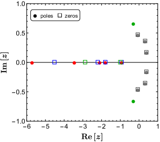
As mentioned in Sec. 3, when building higher-order Padé approximants, it is very important to work with sufficiently high numerical accuracy or, otherwise, the results can be contaminated with spurious poles and zeros. In order to illustrate this, we consider again the use of the genuine Padés to approximate the function $g(z)$ of Eq. (3) for the case $P^{14}_{15}(z)$, which corresponds to 30 parameters. As said before, we do not expect any complex Froissart doublets to appear in this case. This is because $\log(z+2)$ is a Stieltjes function, which generates only real poles in the PAs [43, 44], while the remainder of $g(z)$ is a rational meromorphic function, very easily reproduced by the Padés. However, if insufficient numerical precision is used, the solution to the system of 30 equations can lead to wrong results, in which some of the poles move from the real axis into the complex plane, resembling Froissart doublets (see Sec. 3). These numerical artifacts may appear in a semi-circular pattern [72], as can be clearly seen in Fig. 12, and are similar to the doublets that appear due to the presence of random noise in the input Taylor coefficients [72, 45]. Let us mention that this feature is also visible in the results of Ref. [37], both in the analysis of their toy data and of the lattice data.

In order to circumvent this problem, in the results of Sec. 3, we employed a precision of 30 decimal places for our analysis of the function $g(z)$. In particular, the approximants shown in Fig. 1 were obtained applying the built-in function PadéApproximant of Wolfram Mathematica, imposing this precision. On the contrary, in the above (wrong) solution the same function was used with default precision. Of course, in the presence of spurious pairs of complex zeros and poles generated by round-off errors, it is more difficult to identify the cut of the function $g(z)$. This occurs since some of the poles and zeros that would appear along the cut are now displaced into the complex plane.

Figure 12: Results obtained with insufficient numerical precision (see discussion in the text) for the poles (filled circles) and zeros (empty squares) of $P_{15}^{14}(z)$, built to the Taylor series of $g(z)$ defined in Eq. (3). The poles and zeros that can be identified with genuine poles of $g(z)$ are shown in green, while artifacts are shown in red (poles) and blue (zeros). It is possible to see a number of spurious complex poles and zeros (shown in dark gray), resembling Froissart doublets, that are the result of round-off errors. The correct result can be seen in Fig. 1a.

References

- [1] R. Alkofer and L. von Smekal, The Infrared behavior of QCD Green’s functions: Confinement dynamical symmetry breaking, and hadrons as relativistic bound states, Phys. Rept. 353 (2001) 281 [hep-ph/0007355].
- [2] J. Greensite, An introduction to the confinement problem, vol. 821 of Lecture Notes in Physics. Springer, Berlin, 2011.
- [3] N. Vandersickel and D. Zwanziger, The Gribov problem and QCD dynamics, Phys. Rept. 520 (2012) 175 [1202.1491].
- [4] R. Pasechnik and M. Šumbera, Different Faces of Confinement, Universe 7 (2021) 330 [2109.07600].
- [5] A. Cucchieri and T. Mendes, Numerical test of the Gribov-Zwanziger scenario in Landau gauge, PoS QCD-TNT09 (2009) 026 [1001.2584].
- [6] Y. Aoki et al., FLAG Review 2021, 2111.09849.
- [7] A. Cucchieri, T. Mendes and A. R. Taurines, SU(2) Landau gluon propagator on a lattice, Phys. Rev. D 67 (2003) 091502 [hep-lat/0302022].
- [8] I. L. Bogolubsky, E. M. Ilgenfritz, M. Muller-Preussker and A. Sternbeck, The Landau gauge gluon and ghost propagators in 4D SU(3) gluodynamics in large lattice volumes, PoS LATTICE2007 (2007) 290 [0710.1968].
- [9] A. Cucchieri and T. Mendes, What’s up with IR gluon and ghost propagators in Landau gauge? A puzzling answer from huge lattices, PoS LATTICE2007 (2007) 297 [0710.0412].
- [10] A. Sternbeck, L. von Smekal, D. B. Leinweber and A. G. Williams, Comparing SU(2) to SU(3) gluodynamics on large lattices, PoS LATTICE2007 (2007) 340 [0710.1982].
- [11] P. Boucaud, J. P. Leroy, A. L. Yaouanc, J. Micheli, O. Pene and J. Rodriguez-Quintero, The Infrared Behaviour of the Pure Yang-Mills Green Functions, Few Body Syst. 53 (2012) 387 [1109.1936].
- [12] O. Oliveira and P. J. Silva, The lattice Landau gauge gluon propagator: lattice spacing and volume dependence, Phys. Rev. D 86 (2012) 114513 [1207.3029].
- [13] V. G. Bornyakov, E. M. Ilgenfritz, C. Litwinski, V. K. Mitrjushkin and M. Muller-Preussker, Landau gauge ghost propagator and running coupling in SU(2) lattice gauge theory, Phys. Rev. D 92 (2015) 074505 [1302.5943].
- [14] A. Cucchieri and T. Mendes, Bloch Waves in Minimal Landau Gauge and the Infinite-Volume Limit of Lattice Gauge Theory, Phys. Rev. Lett. 118 (2017) 192002 [1612.01279].
- [15] A. Maas, Describing gauge bosons at zero and finite temperature, Phys. Rept. 524 (2013) 203 [1106.3942].
- [16] C. S. Fischer, Infrared properties of QCD from Dyson-Schwinger equations, J. Phys. G 32 (2006) R253 [hep-ph/0605173].
- [17] A. C. Aguilar, D. Binosi and J. Papavassiliou, The Gluon Mass Generation Mechanism: A Concise Primer, Front. Phys. (Beijing) 11 (2016) 111203 [1511.08361].
- [18] M. Q. Huber, Nonperturbative properties of Yang–Mills theories, Phys. Rept. 879 (2020) 1 [1808.05227].
- [19] M. Peláez, U. Reinosa, J. Serreau, M. Tissier and N. Wschebor, A window on infrared QCD with small expansion parameters, Rept. Prog. Phys. 84 (2021) 124202 [2106.04526].
- [20] N. Dupuis, L. Canet, A. Eichhorn, W. Metzner, J. M. Pawlowski, M. Tissier et al., The nonperturbative functional renormalization group and its applications, Phys. Rept. 910 (2021) 1 [2006.04853].
- [21] J. E. Mandula and M. Ogilvie, The Gluon Is Massive: A Lattice Calculation of the Gluon Propagator in the Landau Gauge, Phys. Lett. B 185 (1987) 127.
- [22] A. Cucchieri, T. Mendes and A. R. Taurines, Positivity violation for the lattice Landau gluon propagator, Phys. Rev. D 71 (2005) 051902 [hep-lat/0406020].
- [23] P. O. Bowman, U. M. Heller, D. B. Leinweber, M. B. Parappilly, A. Sternbeck, L. von Smekal et al., Scaling behavior and positivity violation of the gluon propagator in full QCD, Phys. Rev. D 76 (2007) 094505 [hep-lat/0703022].
- [24] S. Strauss, C. S. Fischer and C. Kellermann, Analytic structure of the Landau gauge gluon propagator, Phys. Rev. Lett. 109 (2012) 252001 [1208.6239].
- [25] S. Strauss, C. S. Fischer and C. Kellermann, Analytic structure of Landau gauge ghost and gluon propagators, Prog. Part. Nucl. Phys. 67 (2012) 239.
- [26] C. S. Fischer and M. Q. Huber, Landau gauge Yang-Mills propagators in the complex momentum plane, Phys. Rev. D 102 (2020) 094005 [2007.11505].
- [27] J. Horak, J. Papavassiliou, J. M. Pawlowski and N. Wink, Ghost spectral function from the spectral Dyson-Schwinger equation, 2103.16175.
- [28] J. Horak, J. M. Pawlowski, J. Rodríguez-Quintero, J. Turnwald, J. M. Urban, N. Wink et al., Reconstructing QCD spectral functions with Gaussian processes, Phys. Rev. D 105 (2022) 036014 [2107.13464].
- [29] J. Horak, J. M. Pawlowski and N. Wink, On the complex structure of Yang-Mills theory, 2202.09333.
- [30] D. Dudal, O. Oliveira, M. Roelfs and P. Silva, Spectral representation of lattice gluon and ghost propagators at zero temperature, Nucl. Phys. B 952 (2020) 114912 [1901.05348].
- [31] S. W. Li, P. Lowdon, O. Oliveira and P. J. Silva, The generalised infrared structure of the gluon propagator, Phys. Lett. B 803 (2020) 135329 [1907.10073].
- [32] D. Binosi and R.-A. Tripolt, Spectral functions of confined particles, Phys. Lett. B 801 (2020) 135171 [1904.08172].
- [33] Y. Hayashi and K.-I. Kondo, Reconstructing confined particles with complex singularities, Phys. Rev. D 103 (2021) L111504 [2103.14322].
- [34] Y. Hayashi and K.-I. Kondo, Reconstructing propagators of confined particles in the presence of complex singularities, Phys. Rev. D 104 (2021) 074024 [2105.07487].
- [35] S. W. Li, P. Lowdon, O. Oliveira and P. J. Silva, Non-perturbative BRST symmetry and the spectral structure of the ghost propagator, Phys. Lett. B 823 (2021) 136753 [2109.10942].
- [36] T. Lechien and D. Dudal, Neural network approach to reconstructing spectral functions and complex poles of confined particles, 2203.03293.
- [37] A. F. Falcão, O. Oliveira and P. J. Silva, Analytic structure of the lattice Landau gauge gluon and ghost propagators, Phys. Rev. D 102 (2020) 114518 [2008.02614].
- [38] O. Oliveira, A. F. Falcão and P. J. Silva, Looking at the analytic structure of Landau gauge propagators, in 38th International Symposium on Lattice Field Theory, 11, 2021, 2111.04320.
- [39] A. Cucchieri and T. Mendes, Constraints on the IR behavior of the gluon propagator in Yang-Mills theories, Phys. Rev. Lett. 100 (2008) 241601 [0712.3517].
- [40] A. Cucchieri and T. Mendes, Constraints on the IR behavior of the ghost propagator in Yang-Mills theories, Phys. Rev. D 78 (2008) 094503 [0804.2371].
- [41] A. Cucchieri, D. Dudal, T. Mendes and N. Vandersickel, Modeling the Gluon Propagator in Landau Gauge: Lattice Estimates of Pole Masses and Dimension-Two Condensates, Phys. Rev. D 85 (2012) 094513 [1111.2327].
- [42] A. Cucchieri, D. Dudal, T. Mendes and N. Vandersickel, Modeling the Landau-gauge ghost propagator in 2, 3, and 4 spacetime dimensions, Phys. Rev. D 93 (2016) 094513 [1602.01646].
- [43] G. A. Baker, Essentials of Padé approximants. Academic Press, New York, 1975.
- [44] G. A. Baker and P. Graves-Morris, Padé approximants. Cambridge University Press, Cambridge, 2nd ed., 1996.
- [45] P. Masjuan, Rational approximations in Quantum Chromodynamics, Ph.D. thesis, Universitat Autònoma de Barcelona, 2010. 1005.5683.
- [46] P. Masjuan and S. Peris, A Rational approach to resonance saturation in large- QCD, JHEP 05 (2007) 040 [0704.1247].
- [47] A. H. Hoang, V. Mateu and S. Mohammad Zebarjad, Heavy Quark Vacuum Polarization Function at and , Nucl. Phys. B 813 (2009) 349 [0807.4173].
- [48] P. Masjuan and S. Peris, Pade Theory applied to the vacuum polarization of a heavy quark, Phys. Lett. B 686 (2010) 307 [0903.0294].
- [49] P. Masjuan and J. J. Sanz-Cillero, Pade approximants and resonance poles, Eur. Phys. J. C 73 (2013) 2594 [1306.6308].
- [50] I. Caprini, P. Masjuan, J. Ruiz de Elvira and J. J. Sanz-Cillero, Uncertainty estimates of the -pole determination by Padé approximants, Phys. Rev. D 93 (2016) 076004 [1602.02062].
- [51] C. Aubin, T. Blum, M. Golterman and S. Peris, Pade approximants and g-2 for the muon, PoS LATTICE2012 (2012) 176 [1210.7611].
- [52] C. Aubin, T. Blum, M. Golterman and S. Peris, Model-independent parametrization of the hadronic vacuum polarization and g-2 for the muon on the lattice, Phys. Rev. D 86 (2012) 054509 [1205.3695].
- [53] D. Boito, P. Masjuan and F. Oliani, Higher-order QCD corrections to hadronic decays from Padé approximants, JHEP 08 (2018) 075 [1807.01567].
- [54] D. Boito, C. Y. London and P. Masjuan, Higher-order QCD corrections to from rational approximants, JHEP 01 (2022) 054 [2110.09909].
- [55] B. Ananthanarayan, D. Das and M. S. A. Alam Khan, QCD static energy using optimal renormalization and asymptotic Padé-approximant methods, Phys. Rev. D 102 (2020) 076008 [2007.10775].
- [56] P. Masjuan, S. Peris and J. J. Sanz-Cillero, Vector Meson Dominance as a first step in a systematic approximation: The Pion vector form-factor, Phys. Rev. D 78 (2008) 074028 [0807.4893].
- [57] P. Masjuan, transition form factor at low-energies from a model-independent approach, Phys. Rev. D 86 (2012) 094021 [1206.2549].
- [58] R. Escribano, P. Masjuan and P. Sanchez-Puertas, and transition form factors from rational approximants, Phys. Rev. D 89 (2014) 034014 [1307.2061].
- [59] P. Masjuan and P. Sanchez-Puertas, and decays into lepton pairs, JHEP 08 (2016) 108 [1512.09292].
- [60] P. Masjuan and P. Sanchez-Puertas, Pseudoscalar-pole contribution to the : a rational approach, Phys. Rev. D 95 (2017) 054026 [1701.05829].
- [61] L. Von Detten, F. Noël, C. Hanhart, M. Hoferichter and B. Kubis, On the scalar form factor beyond the elastic region, Eur. Phys. J. C 81 (2021) 420 [2103.01966].
- [62] V. Gribov, Quantization of non-abelian gauge theories, Nuclear Physics B 139 (1978) 1.
- [63] M. Stingl, Propagation properties and condensate formation of the confined Yang-Mills field, Phys. Rev. D 34 (1986) 3863.
- [64] M. Stingl, A Systematic extended iterative solution for quantum chromodynamics, Z. Phys. A 353 (1996) 423 [hep-th/9502157].
- [65] A. Cucchieri, T. Mendes, O. Oliveira and P. J. Silva, Just how different are SU(2) and SU(3) Landau propagators in the IR regime?, Phys. Rev. D 76 (2007) 114507 [0705.3367].
- [66] A. Cucchieri, T. Mendes, O. Oliveira and P. J. Silva, SU(2) meets SU(3) in lattice-Landau-gauge gluon and ghost propagators, PoS LATTICE2007 (2007) 322 [0710.0344].
- [67] A. Cucchieri, T. Mendes, O. Oliveira and P. J. Silva, Comparing Pure Yang-Mills SU(2) and SU(3) Propagators, Int. J. Mod. Phys. E 16 (2007) 2931 [0711.0509].
- [68] Y. Hayashi and K.-I. Kondo, Complex poles and spectral function of Yang-Mills theory, Phys. Rev. D 99 (2019) 074001.
- [69] K.-I. Kondo, M. Watanabe, Y. Hayashi, R. Matsudo and Y. Suda, Reflection positivity and complex analysis of the Yang-Mills theory from a viewpoint of gluon confinement, Eur. Phys. J. C 80 (2020) 84 [1902.08894].
- [70] P. Lowdon, Non-perturbative constraints on the quark and ghost propagators, Nucl. Phys. B 935 (2018) 242 [1711.07569].
- [71] O. Costin and G. V. Dunne, Conformal and uniformizing maps in Borel analysis, Eur. Phys. J. ST 230 (2021) 2679 [2108.01145].
- [72] H. Yamada and I. Kensuke, A numerical test of padé approximation for some functions with singularity, International Journal of Computational Mathematics 2014 (2014) .
- [73] Particle Data Group collaboration, Review of Particle Physics, PTEP 2020 (2020) 083C01.
- [74] J. C. R. Bloch, A. Cucchieri, K. Langfeld and T. Mendes, Propagators and running coupling from SU(2) lattice gauge theory, Nucl. Phys. B 687 (2004) 76 [hep-lat/0312036].
- [75] A. Cucchieri, Infrared behavior of the gluon propagator in lattice Landau gauge: The Three-dimensional case, Phys. Rev. D 60 (1999) 034508 [hep-lat/9902023].
- [76] A. Cucchieri, T. Mendes and A. Mihara, Ghost condensation on the lattice, Phys. Rev. D 72 (2005) 094505 [hep-lat/0508028].
- [77] P. Boucaud, J. P. Leroy, A. Le Yaouanc, A. Y. Lokhov, J. Micheli, O. Pene et al., Asymptotic behavior of the ghost propagator in SU3 lattice gauge theory, Phys. Rev. D 72 (2005) 114503 [hep-lat/0506031].
- [78] A. Cucchieri, A. Maas and T. Mendes, Exploratory study of three-point Green’s functions in Landau-gauge Yang-Mills theory, Phys. Rev. D 74 (2006) 014503 [hep-lat/0605011].
- [79] J. P. Ma, A Study of gluon propagator on coarse lattice, Mod. Phys. Lett. A 15 (2000) 229 [hep-lat/9903009].
- [80] C. Bernard, C. Parrinello and A. Soni, Lattice study of the gluon propagator in momentum space, Phys. Rev. D 49 (1994) 1585.
- [81] N. Vandersickel, A Study of the Gribov-Zwanziger action: from propagators to glueballs, Ph.D. thesis, Universiteit Gent, 2011. 1104.1315.
- [82] G. D’Agostini, On the use of the covariance matrix to fit correlated data, Nucl. Instrum. Meth. A 346 (1994) 306.
- [83] D. Boito, O. Cata, M. Golterman, M. Jamin, K. Maltman, J. Osborne et al., A new determination of from hadronic decays, Phys. Rev. D 84 (2011) 113006 [1110.1127].
- [84] C. Diaz-Mendoza, P. Gonzalez-Vera and R. Orive, On the convergence of two-point partial padé approximants for meromorphic functions of stieltjes type, Applied numerical mathematics 53 (2005) 39.
- [85] D. Boito, M. Golterman, K. Maltman, S. Peris, M. V. Rodrigues and W. Schaaf, Strong coupling from an improved vector isovector spectral function, Phys. Rev. D 103 (2021) 034028 [2012.10440].
- [86] A. Keshavarzi, D. Nomura and T. Teubner, Muon and : a new data-based analysis, Phys. Rev. D 97 (2018) 114025 [1802.02995].