Abstract

Missing data imputation (MDI) is crucial when dealing with tabular datasets across various domains. Autoencoders can be trained to reconstruct missing values, and graph autoencoders (GAE) can additionally consider similar patterns in the dataset when imputing new values for a given instance. However, previously proposed GAEs suffer from scalability issues, requiring the user to define a similarity metric among patterns to build the graph connectivity beforehand. In this paper, we leverage recent progress in latent graph imputation to propose a novel EdGe Generation Graph AutoEncoder (EGG-GAE) for missing data imputation that overcomes these two drawbacks. EGG-GAE works on randomly sampled mini-batches of the input data (hence scaling to larger datasets), and it automatically infers the best connectivity across the mini-batch for each architecture layer. We also experiment with several extensions, including an ensemble strategy for inference and the inclusion of what we call prototype nodes, obtaining significant improvements, both in terms of imputation error and final downstream accuracy, across multiple benchmarks and baselines.

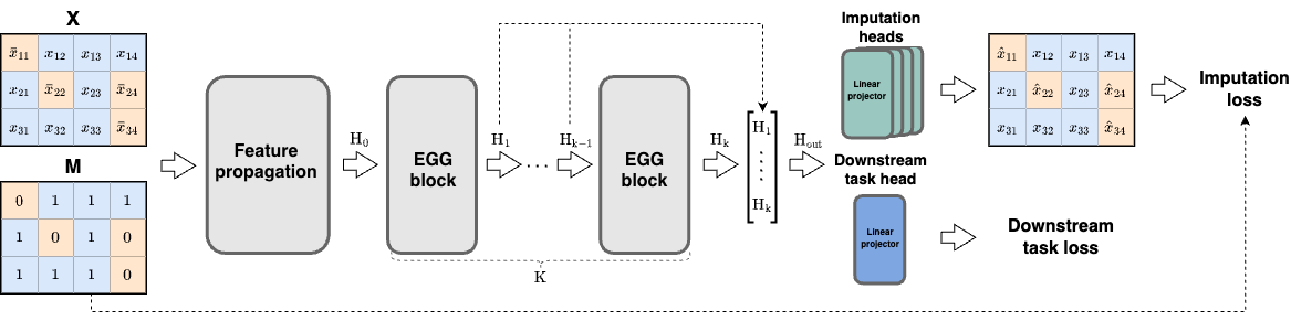
Figure 1: Pipeline: initially, the preprocessed batch $\mathrm{X}$ is encoded with a feature propagation block (Eq. (14)), resulting in the initial representations $\mathrm{H}_{\mathrm{0}}$. These representations are then updated with a sequence of EGG-GAE blocks obtaining ${\mathrm{H}_{\mathrm{k}}}$, $\mathrm{k}\in\{\mathrm{1},\dots,\mathrm{K}\}$. The concatenation of $\{\mathrm{H}_{\mathrm{k}}\}_{\mathrm{k}=\mathrm{1}}^{\mathrm{K}}$ gives the final representation $\mathrm{H}_{\mathrm{out}}$. It is used as the input for the subsequent heads: numerical imputation, categorical imputation, and downstream task one.

1 INTRODUCTION

Missing data imputation is a ubiquitous issue that arises in a variety of domains. Most supervised deep learning methods require complete datasets, but in the real world, datasets often suffer from incompleteness due to access problems or mistakes in data collection (Yoon et al.,, 2016; Yoon et al., 2018b, ; Kreindler and Lumsden,, 2006; Van Buuren,, 2018). Numerous fields thus require missing data imputation (MDI) methods to reconstruct a complete dataset, including biostatistics (Mackinnon,, 2010), epidemiology (Sterne et al.,, 2009), and irregular time-series analysis (Kreindler and Lumsden,, 2006).

Classically, the underlying mechanism giving rise to missing data is categorized into three types (Rubin,, 1976). (1) If the probability of being missing is completely independent of the data, then the data are said to be missing at random (MCAR). (2) Data is said to be missing at random (MAR) if the probability of being missing is the same only within the data-defined groups. (3) If the probability of missing data depends on both observed and unobserved variables, then such data are missing not at random (MNAR).

Predictive approaches to MDI (Bertsimas et al.,, 2017) can be categorized in two families: (i) building a global model for data imputation, or (ii) inferring the missing components employing similar data points to the one having missing values. The second class typically uses advanced k-NN strategies (Acuna and Rodriguez,, 2004). The first class includes simple statistics from the entire dataset (e.g., medians), linear models (Lakshminarayan et al.,, 1996), support vector machines (Wang et al.,, 2006) or, more recently, deep neural architectures (Śmieja et al.,, 2018; Yoon et al., 2018a, ; Nazabal et al.,, 2020; Spinelli et al.,, 2020).

Recently, it was noted that the unification of the two paradigms (i.e., inferring similar data points for each imputation and building global models from the overall dataset) can be beneficial for MDI. This can be done by exploiting Graph Neural Networks (GNNs) (Narang et al.,, 2013; Chen et al.,, 2020; Jiang and Zhang,, 2020; Rossi et al.,, 2021), a novel class of neural networks that can process graph-based data in a differentiable fashion. In particular, the graph imputer neural network (GINN) (Spinelli et al.,, 2020) explored the assumption of endowing tabular data with a graph topology based on a pre-computed similarity between points in the feature space, and then exploiting a GNNs to tackle the MDI problem. However, the proposed GINN model had two limitations. First, the method is tested only on the entire dataset (i.e., no mini-batching is performed, which is challenging with GNNs models), and scaling it up to large datasets is unfeasible due to the quadratic cost of computing the similarity matrix. Second, graph connectivity must be computed beforehand in the feature space employing only those values observed by both data points, requiring the definition of a suitable distance metric and a customized procedure to sparsify the graph.

In general, building a connectivity beforehand as done in GINN was necessary, since the underlying assumption of most GNNs is that the graph topology is given and fixed; thus, convolution-like operations typically amount to modifying the node-wise features by averaging information from the neighbours. However, the hand-crafted connectivity might be sub-optimal and requires a number of hyper-parameters to be defined and manually optimized. Instead, automatically learning the latent graph structure can overcome the limitations of these methods by inferring the underlying graph relationships. Such latent graphs can capture the actual topology of structured data through the downstream tasks, which can be seen as a task-related topology, thus conveying model interpretability. Recently, latent graph imputation has become an important research topic in the GNNs literature, as described in Section 2.2.

Based on these considerations, the main contributions of this paper are as follows. (i) We introduce an end-to-end trainable network architecture to learn the optimal underlying latent graph for tabular data using a novel EdGe Generation Graph AutoEncoder (EGG-GAE) network module. The EGG-GAE module sampling scheme is optimized with respect to downstream task metrics utilizing a straight-through estimator (Jang et al.,, 2016) in the backward pass to ensure its differentiability. (ii) We demonstrate that employing the latent graph predictions for the missing data imputation (MDI) problem induces consistent improvement across a number of datasets in a large experimental evaluation, demonstrating significant improvements over baselines and reaching state-of-the-art performance. (iii) We propose the concept of tabular graph mini-batching along with an ensembling technique to resolve the MDI scalability issues (Miao et al.,, 2022). (iv) We propose a novel concept of learnable prototype nodes which encodes a learnable data representation in the form of an additional set of nodes added to the imputed graph, to provide each data point in the mini-batch with a reliable neighbourhood.

2 RELATED WORKS

Before describing our proposed solution for tabular MDI, we provide a brief overview of related works among three lines: MDI methods for tabular data (Section 2.1), latent graph imputation for GNNs (Section 2.2), and methods to employ GNNs on graphs with missing data (Section 2.3).

2.1 Tabular missing data imputation

MDI algorithms can be categorized depending on whether they are discriminative or generative, univariate or multivariate, and on whether they provide one or multiple imputations for each missing data point. In this work we present a generative model which performs multivariate imputations and can provide multiple imputations for each missing datum.

The imputation strategies can be divided into three categories: 1) statistical; 2) machine learning (ML), and 3) deep learning (DL) based. Statistical methods exploit the observed data to obtain mean, median, or mode estimation of missing data points (Farhangfar et al.,, 2007). Among traditional machine learning imputation approaches, multiple imputation using chained equations (MICE) (Van Buuren and Groothuis-Oudshoorn,, 2011) is considered one of the most flexible and powerful. MICE iteratively imputes each dataset variable while keeping the others constant, selecting one or more observations from a predictive distribution on that variable. Although MICE has performed well in some cases, its underlying assumptions may result in biased forecasts and lower accuracy (Azur et al.,, 2011). ML algorithms include k-nearest neighbours (KNN) (Acuna and Rodriguez,, 2004), decision trees Lakshminarayan et al., (1996), support vector techniques (Wang et al.,, 2006) and several others. In practic

e, these approaches have mixed results compared to more straightforward techniques such as mean imputation (Bertsimas et al.,, 2017). KNN is generally limited to weighted averaging among similar feature vectors, whereas other algorithms are required to build a global dataset model for imputation. DL models include deep denoising autoencoders (Gondara and Wang,, 2018), recurrent neural networks (Bengio and Gingras,, 1995), and generative models (Yoon et al., 2018a, ; Nazabal et al.,, 2020). Multilayer nonlinear computation allows these methods to capture more complex correlations in data, however, they still require building a global model from the dataset while ignoring potentially significant contributions from similar points. GINN (Spinelli et al.,, 2020) addressed the problem of leveraging both the global aspect of the dataset and local dependencies between different data points utilizing GNNs. GINN requires the calculation of a pre-defined similarity matrix on the entire dataset in feature space, which is unfeasible for most real-world databases.

2.2 Latent graph learning

GNNs exploit the general idea of localized message-passing, e.g., using graph convolutional layers (Kipf and Welling,, 2017), GraphSAGE (Hamilton et al.,, 2017), edge convolutions (Gilmer et al.,, 2017), and graph attention (Veličković et al.,, 2018). In their basic formulation, GNNs layers require graph connectivity to be provided as input to the model. Mini-batches of data can be formed by sampling several graphs from a pool of graphs or sampling sub-graphs with a fixed number of nodes or connections from the original graph (Zou et al.,, 2019; Cong et al.,, 2020). The common disadvantages of these methods are that they require a given or fixed input graph and the requirement of a sparse graph to make the approach computationally feasible, especially for large graphs. Recently, methods which do not assume given or fixed graph connectivity were proposed. Such methods construct the graph dynamically during training. Wang et al., (2019) proposed Dynamic Graph CNNs (DGCNN) using KNN to construct the graph on-the-fly in the feature space of the neural network. Later, a graph learning model was proposed in Cosmo et al., (2020) that builds a probability graph as a weighted adjacency matrix for an optimal classification result. Thus, the graph is built in a fully connected manner, implying that the model cannot exploit the possible sparseness of the graph. A more general Differential Graph Module (DGM) (Kazi et al.,, 2022) explicitly models sparse latent graphs employing the Gumbel-top-k trick (Kool et al.,, 2019), overcoming the dense graph limitations by fixing the number of neighbours for each node which allows working with bigger graphs. We take inspiration from DGM for our sampling scheme, and we detail the major differences in Section 4.

2.3 Node feature imputation in GNNs

GNNs models typically cannot deal with attribute-incomplete graph data directly, where rows represent nodes and columns feature channels. However, in real-world scenarios, features are often only observed for a subset of the nodes. Several works address missing node features in graph machine learning tasks. SAT (Chen et al.,, 2020) uses transformer-like models for feature completion followed by independent GNNs to solve the downstream task, which leads to a sub-optimal solution. GCNMF (Taguchi et al.,, 2021) overcomes this limitation by employing a Gaussian mixture model (GMM) to represent missing node features and jointly learns the GMM and GNNs parameters, however, this significantly increases the number of trainable parameters, implying high computational cost. PaGNNs introduced partial aggregation functions to propagate only the observed features (Jiang and Zhang,, 2020). However, these cannot scale to large graphs (Rossi et al.,, 2021). Recently a discrete diffusion-based feature reconstructions framework was proposed, which leads to a simple, fast and scalable iterative algorithm (Rossi et al.,, 2021), though the method is designed to work for homophilic graphs.

3 PROBLEM FORMULATION

Let the matrix $\mathbf{X}=\{\mathbf{x}_{i}\}_{i=1}^{\mathrm{N}}$ denote a $\mathrm{d}$-dimensional dataset and $\mathbf{Y}$ represents its corresponding target vector. Without loss of generality, we assume each data vector $\mathbf{x}_{i}$ contains numerical variables referred to $\mathrm{d}\in\{1,\dots,\mathrm{d}_{\mathrm{n}}\}$ and categorical variables indexed by $\mathrm{d}\in\{\mathrm{d}_{\mathrm{n+1}},\dots,\mathrm{d}_{\mathrm{n}}+\mathrm{d}_{\mathrm{c}}\}$ with $\mathrm{d}_{\mathrm{n}}+\mathrm{d}_{\mathrm{c}}=\mathrm{d}$. We assume that each $\mathrm{d}_{\mathrm{th}}$ categorical variable takes values among $\mathrm{C}_{\mathrm{d}_{\mathrm{th}}}$ classes. The dataset $\mathbf{X}$ is referred as mixed if $\mathrm{d}_{\mathrm{n}}>0,\mathrm{d}_{\mathrm{c}}>0$, numerical if $\mathrm{d}_{\mathrm{c}}=0$ and categorical when $\mathrm{d}_{\mathrm{n}}=0$. By definition some percentage $\mathrm{I}_{\mathrm{init}}\in[0,1)$ of dataset entries $\mathrm{x}_{ij}\in\mathbf{X}$ are missing (corrupted). We associate a binary matrix $\mathbf{M}\in\{0,1\}^{\mathrm{N}\times\mathrm{N}}$ to identify missing and observed variables, where $1$ corresponds to the observed values, and $0$ indicates missing ones. Note that the corruption process can be of many types: MCAR, MNAR, MAR, and it is generally unknown to the user. The imputation process aims to provide a plausible estimation $\hat{\mathrm{x}}_{ij}$ for unobserved values $\mathrm{x}_{ij}$, such that (i) the imputed dataset $\widehat{\mathbf{X}}$ would be as close as possible to the real complete dataset (if such exists), (ii) the imputed dataset $\widehat{\mathbf{X}}$ has to achieve strong downstream task performance if adopting $\widehat{\mathbf{X}}$ as input to predict the corresponding target vector $\mathbf{Y}$.

Dataset preprocessing

We assume that the dataset $\mathbf{X}$, by definition, is properly normalized and corrupted in advance, hence the corresponding corruption matrix $\mathbf{M}$ is determined. Training different imputation approaches discussed in this paper requires distinct data preprocessing strategies. A straightforward way is to employ statistics of observed values. In our work, numerical values are initially assessed with mean statistics, while categorical ones are approximated with the corresponding most frequent class unless otherwise stated. Some of the imputation baselines discussed in this paper also require one-hot encoding of categorical values. The preprocessed dataset is denoted as $\overline{\mathbf{X}}$, which is the input to the subsequent EGG-GAE module.

4 METHOD

We propose a general solution for the tabular data MDI problem based on graph representation learning, whose overall pipeline is depicted in Fig. 1. At every iteration, a mini-batch of data is sampled and preprocessed, according to the procedure described in Section 4.1. This mini-batching is necessary, as it allows the algorithm to scale to large datasets. Next, we build a graph where each node is a row of the sampled mini-batch, and its corresponding node features are a non-linear mapping of the original inputs. The connectivity between nodes is learned through a differentiable sampling procedure, instead of being fixed as in previous works (e.g., (Spinelli et al.,, 2020)). We describe different variations of this last component in Section 4.2. We also propose two extensions to this basic architecture, i.e., ensembling and what we call prototype nodes, in Section 4.3. The entire system is trained end-to-end with a combination of imputation losses and a downstream classification loss, as described in Section 4.4.

4.1 Mini-batch preprocessing

Like in Spinelli et al., (2020), we turn MDI into a predictive task by employing a surrogate task, we randomly remove elements from the mini-batch and impute them to enable our model to reconstruct missing values. In contrast to denoising auto-encoders (Vincent et al.,, 2008), we only predict the removed elements rather than reconstructing the entire input. In order to obtain a surrogate batch-level corruption matrix $\mathrm{M}$ we use the MCAR mechanism to mask a certain percentage $\mathrm{I}_{\mathrm{b}}\in[0,1-\mathrm{I}_{\mathrm{init}})$ of the sampled batch $\mathrm{X}\sim\overline{\mathbf{X}}$. Precomputed statistics replace numerical masked values, while unobserved categorical entries are replaced with auxiliary tokens. We replace each categorical variable with a trainable dense embedding, whose size is a hyperparameter. Note that initial missing values, which have to be imputed during the inference, are represented as observed variables in the surrogate batch-level corruption matrix $\mathrm{M}$. The concatenation of the preprocessed batch parts: categorical $\mathrm{X}^{\mathrm{c}}$ and numerical $\mathrm{X}^{\mathrm{n}}$, yields the final preprocessed batch. In order to avoid cumbersome notation, we refer to the final batch representation as $\mathrm{X}$.

4.2 Architecture

The core feature of the proposed EGG-GAE model is the EGG block, which endows the tabular representation of the sampled mini-batch with a graph topology in order to predict the missing values with a GNN module. The general EGG module comprises three components, as depicted schematically in Fig. 2: (i) a node projector transforms input features $\mathrm{H}_{\mathrm{k}}$ by projecting each row into a new space $\mathrm{H}^{\mathrm{g}}_{\mathrm{k}}$ that we call the graph embedding space; (ii) A sampler, which obtains the edge set $\mathcal{E}_{\mathrm{k}}$ by sparsifying all possible edges between nodes; (iii) a GNN head that operates on the obtained graph $\mathcal{G}=(\mathrm{H}_{\mathrm{k}},\mathcal{E}_{\mathrm{k}})$. The EGG blocks can be stacked subsequently while their outputs concatenated to obtain the final representation $\mathrm{H}_{\mathrm{out}}$. In the following, we describe two variations of EGG blocks: the standard EGG blocks sample each edge independently, and a restricted $k$-EGG block that samples exactly $k$ neighbors for each node.

Before the first EGG block, the preprocessed batch $\mathrm{X}$ is encoded via an initial mapping function:

$$\mathrm{H}_{0}=\mathrm{MLP}_{\mathrm{FP}}(\mathrm{X})$$ (1)

where $\mathrm{MLP}_{\mathrm{FP}}$ is a two-layer MLP with a ReLU activation and batch normalization in between.

EGG

Each EGG block first projects the input $\mathrm{H}_{\mathrm{k}}$ with an additional row-wise operation, obtaining:

$$\mathrm{H}^{\mathrm{g}}_{\mathrm{k}}=\mathrm{MLP}_{\mathrm{k}}(\mathrm{H}_{\mathrm{k}})$$ (2)

where $\mathrm{MLP}_{\mathrm{k}}$ has the same architecture as $\mathrm{MLP}_{\mathrm{FP}}$. The sampler block represents pairwise edge relations of the projected $\mathrm{H}^{\mathrm{g}}_{\mathrm{k}}$ by first forming a probability matrix $\mathrm{P}$ where the $i$-th, $j$-th element is computed as:

$$\mathrm{P}_{ij}=\exp^{||{\mathrm{h}}_{i}-{\mathrm{h}}_{j}||^{2}}$$ (3)

where ${\mathrm{h}}_{i},{\mathrm{h}}_{j}$ are $i$-th and $j$-th rows of matrix $\mathrm{H}^{\mathrm{g}}_{\mathrm{k}}$. Each element of $\mathrm{P}_{ij}$ represents the probability of sampling edge $(i,j)$ in the output graph. In order to sample an undirected graph, corresponding to a strictly upper triangular adjacency matrix $\tilde{\mathrm{A}}_{\mathrm{k}}$, we combine a Gumbel-Softmax trick (Jang et al.,, 2016) for sampling from $\mathrm{P}$ with masking:

$$\tilde{\mathrm{A}}_{ij}=(1+\mathrm{exp}(\nicefrac{{(\log{(\mathrm{P}_{ij}\odot\mathrm{J}_{ij})}+\mathrm{G}_{ij}\odot\mathrm{J}_{ij})}}{{\tau}}))^{-1}$$ (4)

where $\tau$ is a separate temperature hyperparameter, $\mathrm{J}$ is a strictly upper triangular matrix with ones above the main diagonal, $\odot$ is the Hadamard product, and $\mathrm{G}_{ij}\sim\text{Gumbel}(0,1)$. We obtain a sparse matrix by then thresholding $\tilde{\mathrm{A}}_{\mathrm{k}}$ at $0.5$. The final sparse unweighted adjacency matrix $\mathrm{A}_{\mathrm{k}}=$ is computed as:

$$\mathrm{A}_{\mathrm{k}}=\tilde{\mathrm{A}}_{\mathrm{k}}+\tilde{\mathrm{A}}_{\mathrm{k}}^{\mathrm{T}}+\mathrm{I}$$ (5)

where $\mathrm{I}$ is the identity matrix. In order to have a valid gradient for back-propagation with respect to the thresholding operation, we use a straight-through estimator in the backward pass (Jang et al.,, 2016) to allow the gradient flow through the sampling scheme. The final input of the GCN head is then a sparse unweighted adjacency matrix $\mathrm{A}_{\mathrm{k}}$ along with the corresponding feature representation $\mathrm{H}_{\mathrm{k}}$. The updated node representation $\mathrm{H}_{\mathrm{k+1}}$ is computed as:

$$\hat{\mathrm{H}}_{\mathrm{k+1}} =\mathrm{GCN}(\mathrm{H}_{\mathrm{k}},\mathrm{A}_{\mathrm{k}})$$ (6)

$$\mathrm{H}_{\mathrm{k+1}} =\mathrm{LayerNorm}(\hat{\mathrm{H}}_{\mathrm{k+1}}+\mathrm{H}_{\mathrm{k}})$$ (7)

where $\mathrm{GCN}$ is a graph convolutional layer (Kipf and Welling,, 2017) or any other message-passing layer that operates on the graph connectivity.

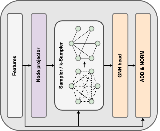
Figure 2: Schematic depiction of the EGG module.

$\boldsymbol{k}$-EGG

We also explore a variant of EGG, called $k$-EGG, which is more directly inspired to the sampling procedure in Kool et al., (2019). It forces a sparsity of the adjacency matrix by limiting the number of neighbours sampled per node to a fixed constant $k$. For each row $i$ of $\mathrm{A}_{\mathrm{k}}$, instead of thresholding each entry, we extract the first $k$ edges corresponding to the $k$ highest values, obtaining $\{(i,j_{1}),\dots,(i,j_{k})\}_{i=1}^{\mathrm{n}}$ and filling with ones the corresponding positions of matrix $\tilde{\mathrm{A}}_{\mathrm{k}}\in\{0,1\}^{\mathrm{n}\times\mathrm{n}}$. The unweighted adjacency matrix $\mathrm{A}_{\mathrm{k}}$ is computed as in Eq. (5).

Comparisons with DGM

Our graph sampling procedure is inspired to the recently proposed DGM block (Kazi et al.,, 2022), with a number of important differences that we mention here. First, DGM was designed for a graph scenario where the full set of nodes is available beforehand and a single underlying graph connectivity is assumed to exist. Instead, we work on randomly sampled mini-batches of data coming from a generic tabular dataset. Second, since the size of mini-batch is a user-defined parameter, we use directly the straight-through estimator in the backward pass, avoiding an additional surrogate loss as in Kazi et al., (2022). The proposed module does not require to limit the output dimensions of the node projector to small values, hence obtaining greater model expressivity. Finally, the GNN head in this paper follows a design with skip-connections and layer normalization.

4.3 Extensions to the basic formulation

We describe here two simple extensions of the model that we have found to work consistently better in our experimental evaluation.

Ensembling

The proposed model has two sources of stochasticity: mini-batch sampling and continuous relaxation of discrete random variables (the edge sampling procedure). We propose to exploit this stochasticity during inference by sampling the batches from the test set until each datum (node) has the desired number of predictions, so that each node has multiple predictions relying on different neighbourhoods. In the classification case, we select the maximum average soft prediction, whereas we use the mean prediction for the regression case.

Prototype nodes

In this paper, we also propose to use trainable prototype nodes which we refer to as $\mathrm{H}_{\mathrm{pr}}$. Applying mini-batching to tabular or graph-structured data may lead in exceptional cases to a lack of data expressiveness during the forward pass due to the same sources of stochasticity mentioned above. For instance, in the case of tabular data, there is no guarantee that the sampled mini-batch composes a reliable set of neighbours for the particular datum prediction. Therefore, prototype nodes are designed to encode common data patterns and allow each data point to have reliable neighbours regardless of the sampled mini-batch. The number of prototypes nodes is a hyperparameter. We initialize the prototypes nodes randomly. However, other strategies such as data mean can be applied. The prototype nodes are then added to $\mathrm{H}_{k}$ before every EGG block. $\mathrm{H}_{\mathrm{pr}}$ does not participate explicitly in the objective function while contributing as sampled neighbours.

4.4 Objective

The objective function consists of two main terms: downstream loss and imputation loss. The downstream loss $\mathcal{L}_{\mathrm{task}}$ paired with the model construction allows to perform end-to-end training, including sampling scheme optimization (in contrast to the DGM paper (Kazi et al.,, 2022)). In the experiments, we use classification task datasets. Therefore, the proposed model is optimized through a cross-entropy loss.

The imputed data $\widehat{\mathrm{X}}$ along with the network predictions $\widehat{\mathrm{Y}}$ are obtained through representation $\mathrm{H}_{\mathrm{out}}$ as:

$$\widehat{\mathrm{X}} =[\mathbf{H}^{\mathrm{n}}(\mathrm{H}_{\mathrm{out}}),\mathbf{H}^{\mathrm{c}}_{i}(\mathrm{H}_{\mathrm{out}})]$$ (8)

$$\widehat{\mathrm{Y}} =\mathbf{H}^{\mathrm{task}}(\mathrm{H}_{\mathrm{out}})$$ (9)

where $\mathbf{H}^{\mathrm{n}},\{\mathbf{H}^{\mathrm{c}}_{i}\}_{i=1}^{\mathrm{c}},\mathbf{H}^{\mathrm{task}}$ are linear projectors, acting row-wise on the input matrix $\mathrm{H}_{\mathrm{out}}$. The downstream task loss $\mathcal{L}_{\mathrm{task}}$ depends on the dataset, in our case that is cross entropy. Note that downstream task loss implicitly contributes to finding the best solution for the imputation problem and latent graph representation learning. The prototype nodes do not participate in any losses explicitly. However, implicit contribution through neighbour batch nodes allows the gradient to flow backwards and learn their representation. The mini-batch masking procedure introduces a surrogate objective to simulate the presence of missing data for which the reconstruction loss is computed. We optimize the MDI solution with the sum of Eq. (10) and (11), $\mathrm{M}^{\mathrm{n}},\mathrm{M}^{\mathrm{c}}$ are numerical and categorical parts of surrogate batch-level corruption matrix $\mathrm{M}$ corresponding to $\mathrm{X}^{\mathrm{n}},\mathrm{X}^{\mathrm{c}}$ subsequently.

$$\mathcal{L}^{\mathrm{n}}_{\mathrm{imp}} =\frac{\mathrm{MSE}(\mathrm{X}^{\mathrm{n}}\odot\mathrm{M}^{\mathrm{n}},\widehat{\mathrm{X}}^{\mathrm{n}}\odot\mathrm{M}^{\mathrm{n}})}{\sum\mathrm{M}^{\mathrm{n}}}$$ (10)

$$\mathcal{L}^{\mathrm{c}}_{\mathrm{imp}} =\frac{\mathrm{CrossEntropy}(\mathrm{X}^{\mathrm{c}}\odot\mathrm{M}^{\mathrm{c}},\widehat{\mathrm{X}}^{\mathrm{c}}\odot\mathrm{M}^{\mathrm{c}})}{\sum\mathrm{M}^{\mathrm{c}}}$$ (11)

$$\mathcal{L}_{\mathrm{h}} =\sum_{i=1}^{\mathrm{N}}\sum_{j=1}^{\mathrm{N}}\bar{\mathrm{a}}_{ij}{\mathrm{a}}_{ij}$$ (12)

Graph learning generally assumes a homophilic structure of the data, i.e., similar patterns are connected with a higher probability, which in our case means that we expect patterns of the same class to be linked. We can explicitly enforce homophily by penalising interclass entries within the sampled adjacency matrix $\mathrm{A}$. The target vector $\mathbf{Y}$ provides an idealized adjacency matrix $\mathrm{A}_{\mathbf{Y}}$, where $\mathrm{A}_{\mathbf{Y}_{ij}}=1$ if $\mathbf{Y}_{i}$ and $\mathbf{Y}_{j}$ belong to the same class, otherwise zero. The complement of the idealized adjacency is denoted as $\bar{\mathrm{A}}_{\mathbf{Y}}$. Equation (12) represents the penalization term, where $\bar{\mathrm{a}}_{ij}\in\bar{\mathrm{A}}_{\mathbf{Y}}$ and $\mathrm{\mathrm{a}}_{ij}\in\mathrm{A}$. The final objective $\mathcal{L}$ is computed as a weighted combination of losses (10-12):

$$\mathcal{L}=\alpha\mathcal{L}_{\mathrm{task}}+\beta(\mathcal{L}^{\mathrm{n}}_{\mathrm{imp}}+\mathcal{L}^{\mathrm{c}}_{\mathrm{imp}})+\gamma\mathcal{L}_{\mathrm{h}}$$ (13)

where $\alpha$, $\beta$, $\gamma$ are loss weights.

5 EXPERIMENTS AND RESULTS

The primary experimental comparison is discussed in Section 5.1, whereas in Section 5.2, we concentrate on architectural ablations. All experiments are conducted at the following noise levels: $10\%,20\%,30\%,40\%$, and $50\%$.

Datasets

We validate our method on 15 datasets from the UCI repository by artificially introducing missing values using MCAR, MNAR, or MAR mechanisms (the setup for MAR and MNAR is replicated from Muzellec et al., (2020)). Table 1 displays the aggregate statistics for the datasets. The training and test parts of the SUSY dataset were subsampled so that they could be compared to the majority of imputation baselines. The remaining datasets are divided into training sets (70%) and validation sets (30%). To satisfy a real-world scenario, we optimise the model with respect to additional noise introduced into the validation set (using the MCAR mechanism regardless of the source of initial missingness) and report the results concerning the initially missing values. Following the relevant literature, we evaluate the imputation and post-imputation prediction performance for each experiment.

Table 1: Dataset statistics. For each dataset, we provide the number of samples, the number of numerical features, and the number of categorical datasets.

Data type	Dataset	#Samples	#Num.Fs.	#Cat.Fs.
Numerical	Yeast	1484	8	0
	Wireless	2000	7	0
	Abalone	4177	8	0
	Wine-quality	4898	11	0
	Page blocks	5473	10	0
	Electrical grid stability	10000	14	0
	SUSY (small)	25000	18	0
Mixed	Anuran	7195	22	3
	Default credit card	30000	14	10
	Adult	32561	6	8
Categorical	Car	1728	0	6
	Phishing websites	2456	0	9
	Letter	20000	0	16
	Chess	28056	0	6
	Connect	67557	0	42

Algorithms

In the experiments the proposed architectures EGG-GAE and $k$-EGG-GAE, are compared with two statistical imputation methods: Mean (Little and Rubin,, 2019), KNN (Troyanskaya et al.,, 2001), two machine learning imputation approaches: MICE (Van Buuren and Groothuis-Oudshoorn,, 2011), MissForest (MF) (Stekhoven and Bühlmann,, 2012) and four deep learning approaches: MIDA (Gondara and Wang,, 2018), GINN (Spinelli et al.,, 2020), GAIN (Yoon et al., 2018a, ), and NN (the proposed architecture wherein EGG block is substituted with an MLP one that is identical to $MLP_{\mathrm{FP}}$). To provide a fair comparison with the baselines, we apply the hyper-parameters and data preprocessing steps from the original papers for all datasets. The proposed models and NN baseline utilize the data pipeline described in this paper.

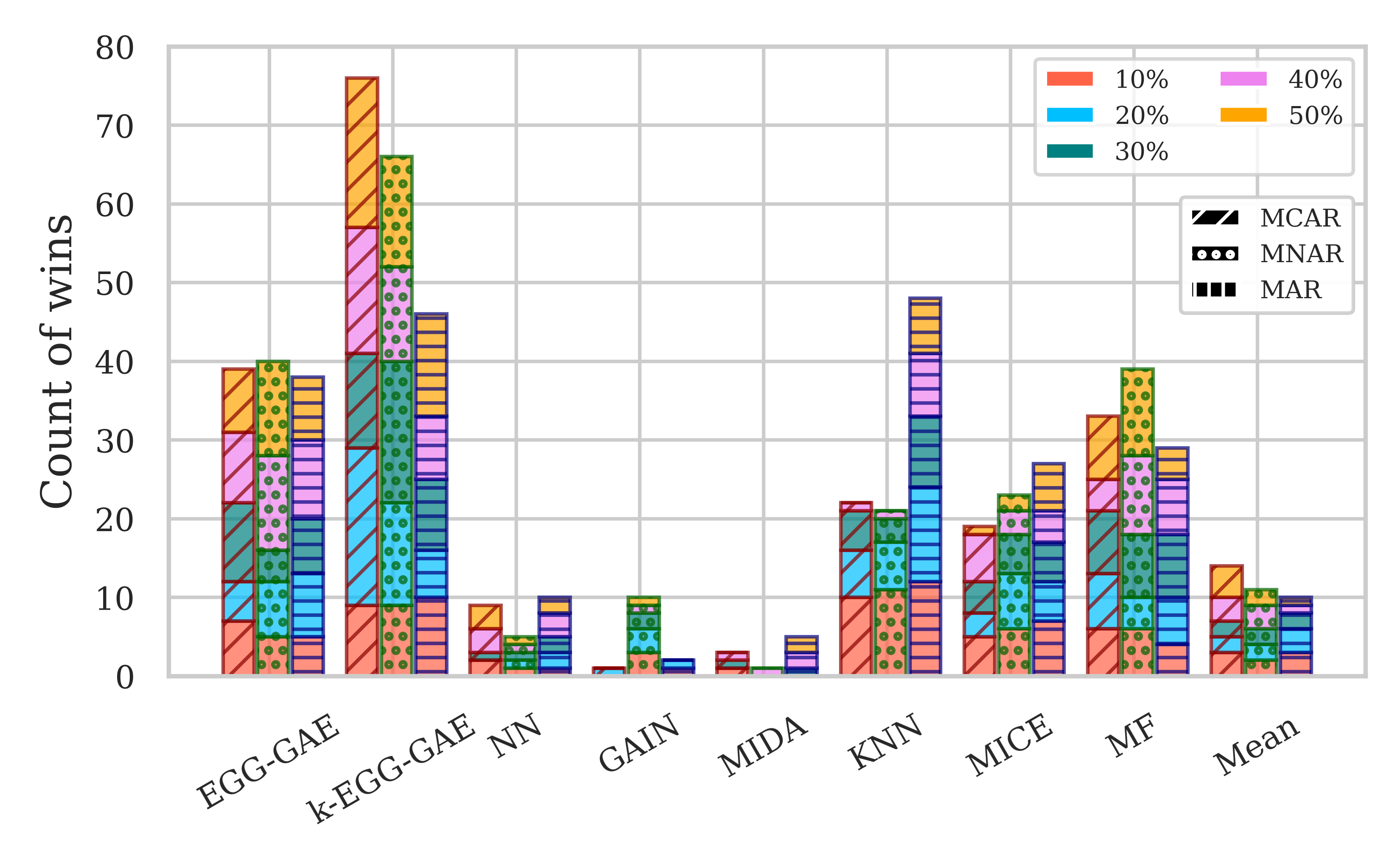
(a) Unified count of wins

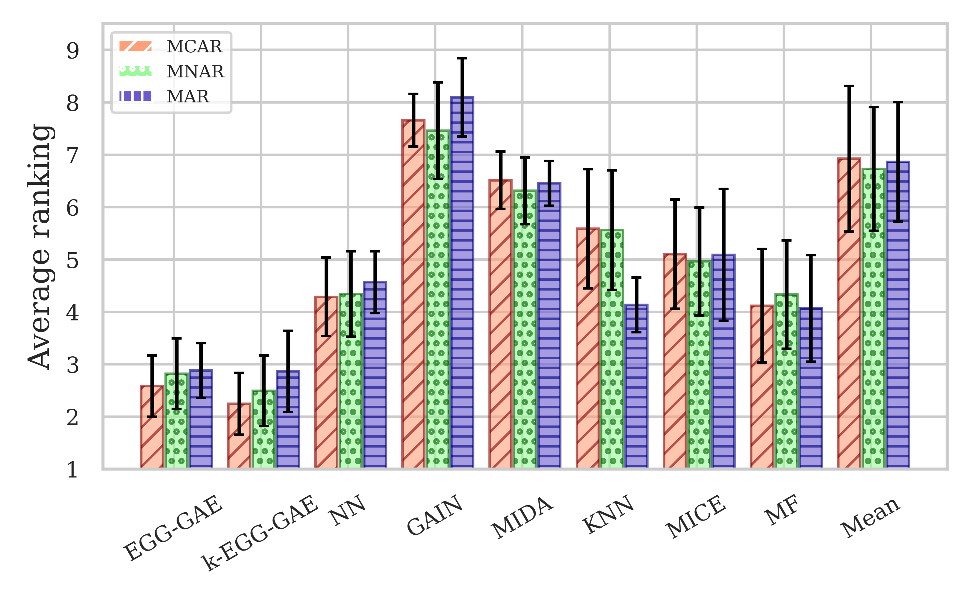
(b) Unified average ranking

Figure 3: Unified average ranking computed for the MCAR, MNAR, and MAR scenarios.

Proposed architecture details

The surrogate batch level corruption is introduced with the MCAR mechanism and $\mathrm{I}_{b}=0.2$. The number of EGG blocks is equal to $1$. The hidden representations of all MLPs (feature propagation block and node mapper) are equal to $300$. The batch size is equal to $300$. The regularization homophily parameter is equal to $0.1$. The temperature parameter $\tau$ linearly decrease from $0.5$ to $0.01$. During inference, the ensembling parameter is equal to $5$. EGG-GAE and $k$-EGG-GAE share the majority of architectural hyperparameters, and for $k$-EGG-GAE we fix the number of sampled neighbours per node at $k=5$. We utilize RMSprop for the optimization with the learning rate equal to $0.0001$.

5.1 Imputation

The main set of experiments addresses the imputation reconstruction and predictive performance of the proposed networks in comparison to baseline algorithms utilising the MCAR, MNAR, and MAR mechanisms. The predictive performance of an MDI solution for tabular data is typically measured by classical machine learning (ML) algorithms for a downstream task. To assess post-imputation downstream task performance we employ random forest Breiman, (2001). We show a schematic result with a unified count of wins and a unified average ranking that takes all levels of noise into account.

The unified count of wins shows the summary for each level of noise and missing mechanism (MCAR, MNAR and MAR). It represents the unified number of times that each method achieves the best performance with respect to the imputation or post-imputation task metrics, i.e., the lowest for RMSE, MAE and the highest in imputation and predictive accuracy. To compute the average ranking we first rank the model for each dataset according to the performance metric. The average ranking is then calculated by averaging the obtained rankings across all datasets. We obtain a separate average ranking for each level of noise, resulting in a matrix consisting of average rankings for every level of noise. The unified average ranking represents multiple average rankings based on a variety of performance metrics and is displayed as a bar graph with error bars. The bar height represents the mean of average rankings regarding the performance metrics and noise levels, while the error bars show corresponding variations. Note that GINN does not participate in the unified count of wins or unified average ranking, because execution time of GINN for big datasets is unfeasible within a reasonable amount of time. The full results for the scenario in which $20\%$ of the entries are missing can be found in the supplementary material, Appendix B, where GINN model is represented as well.

In Fig. 3, it is evident that the suggested models outperform the baselines for every missing mechanism, especially for higher noise levels. Fig. 3(a) shows that $k$-EGG-GAE achieves the best score considerably more often than EGG-GAE, especially for MCAR and MNAR scenarios. Aggregating the results across every noise level, we observe that the EGG-GAE and $k$-EGG-GAE together accumulate $53\%,49\%,39\%$ of the best cases against the $15\%,18\%$, and $22\%$ of its best competitor for the MCAR, MNAR and MAR mechanisms, respectively. The machine learning baselines (KNN, MICE, and MF) are the strongest competitors, achieving the best performance in $33\%,40\%$, and $48\%$ of the cases (cumulatively) for the MCAR, MNAR, and MAR scenarios, accordingly. In Fig.3(b), we can see that the proposed model framework using MLP instead of EGG (referred to as NN) performs just as well as MF on average, even though it rarely achieves the highest score. In addition, we can see that the proposed EGG-GAE and $k$-EGG-GAE models stay roughly on par.

5.2 Ablation experiments

We perform ablation studies over the numerical datasets (reported in Table 1). The ablation study examines model architecture alterations, evaluating ensembling and prototype nodes. The results are averaged across five runs and presented as unified average rankings based on end-to-end accuracy, RMSE and MAE. In Section 5.2.1 we analyse the proposed methods further by comparing training/inference timings for various neural baselines.The architectural experiments can be found in the suplementary materials, Appendix A.

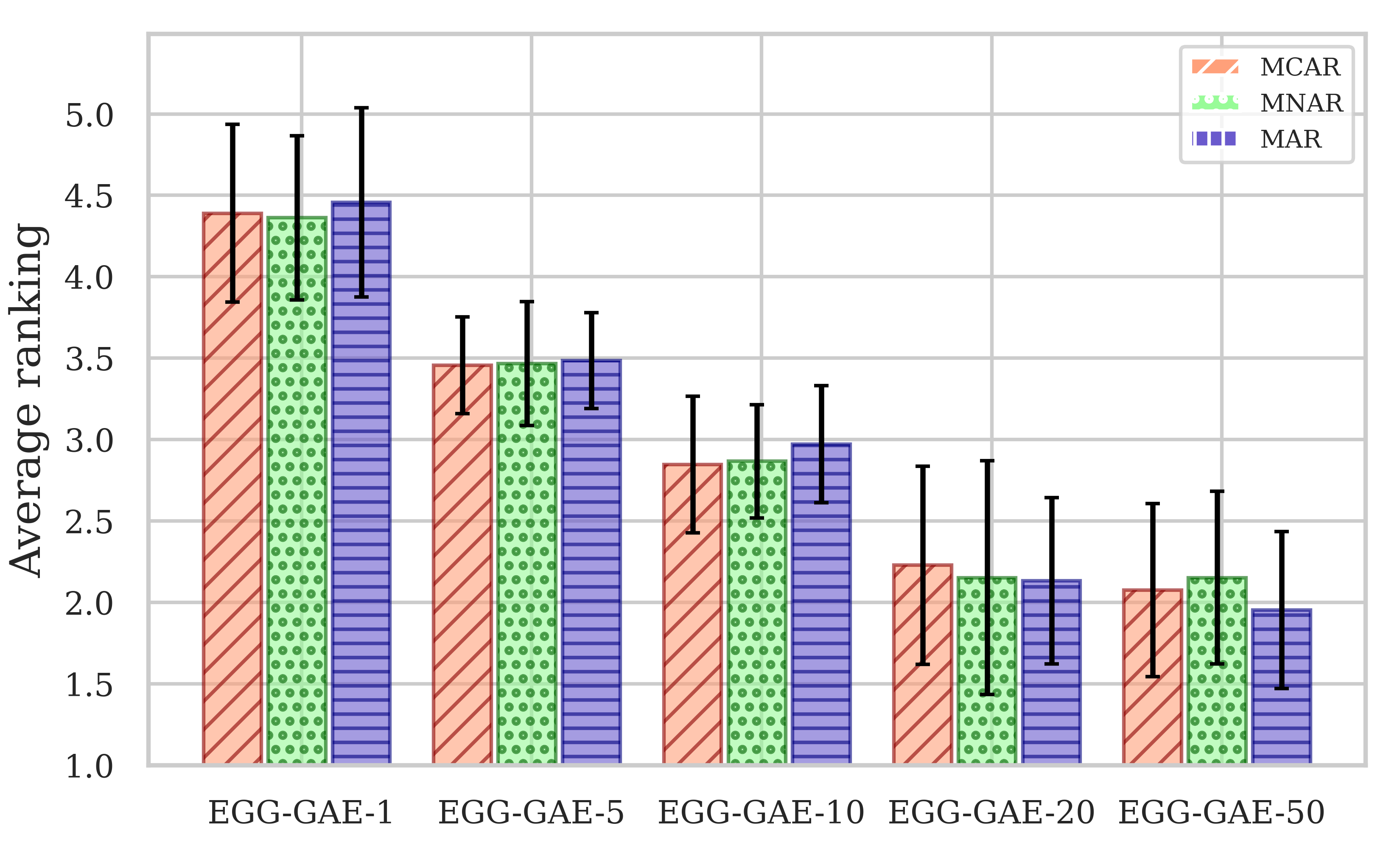
(a) Ensembling

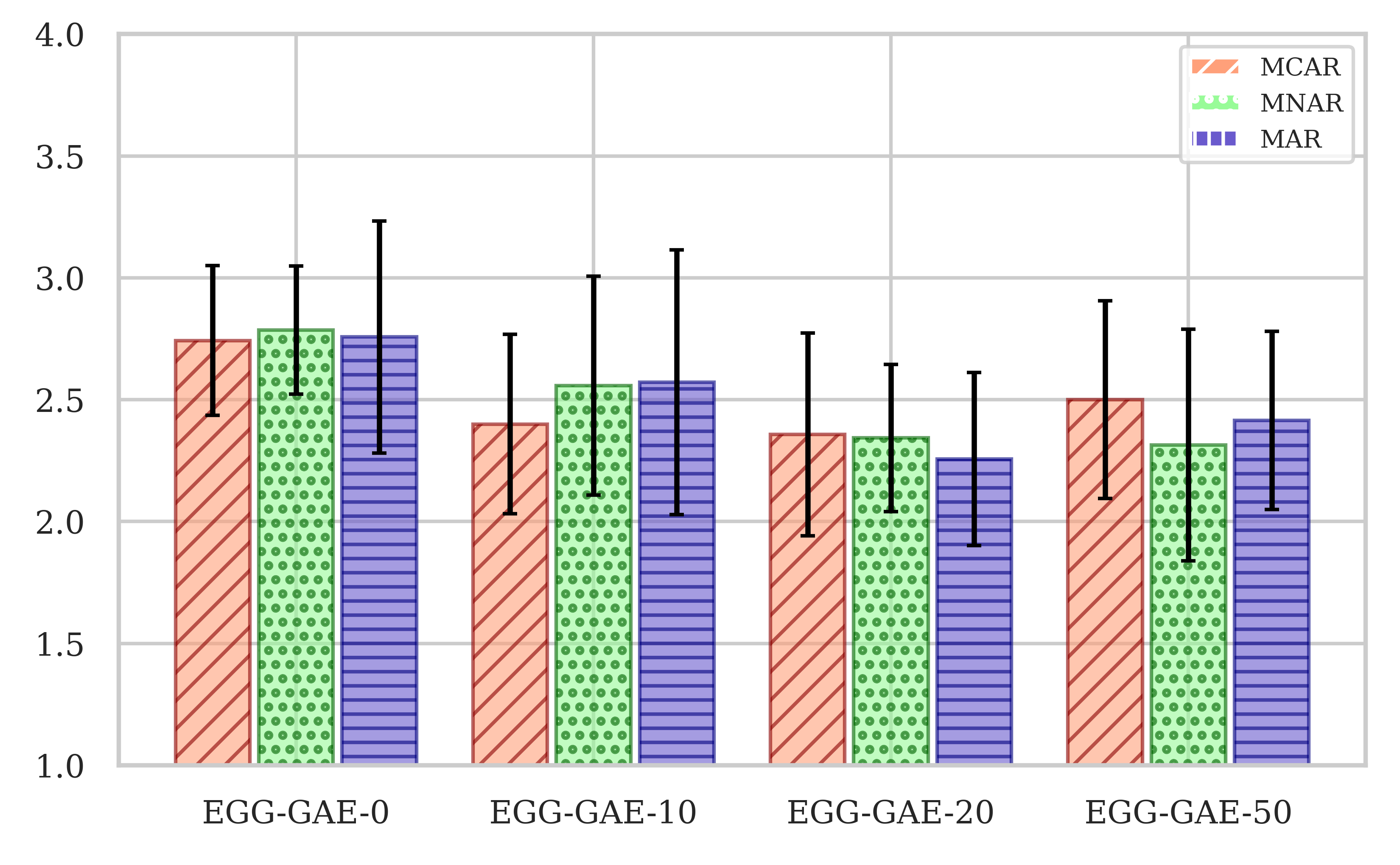
(b) Prototype nodes

Figure 4: Unified average ranking computed for the MCAR, MNAR, and MAR scenarios. A value following the model’s name indicates the variable parameter: a number of prototype nodes or a number ensembling iterations.

Figure 4(a) shows that performing ensembling during inference enhances the performance of downstream and MDI problems regardless of missingness mechanisms. We can see that increasing the number of ensembling iterations on average causes improvement for every type of missingness, as hypothesized. Both EGG-GAE-20 and EGG-GAE-50 have close mean values, while the corresponding variations share the same interval (around $[1.3,2.8]$); this suggests that the plateau is reached when the number of iterations surpasses 20. We argue that performing ensembling during the inference leads to (i) reliable performance (ii) enhancing the performance of downstream and MDI problems. Figure 4(b) demonstrates that the models with learnable prototype nodes (EGG-GAE-10, EGG-GAE-20, and EGG-GAE-50) have a lower mean average ranking compared to the model without them (EGG-GAE-0), independent of the missingness mechanisms scenario. Increasing the number of prototype nodes helps to achieve better performance. However, we can see that introducing a significant number of prototype nodes might worsen the performance (EGG-GAE-50). We believe that the number of prototype nodes should be at least equal to the number of classes of downstream tasks. However, adding too many prototype nodes can impair the performance. We believe it affects the sampling scheme by increasing the likelihood that the graphs will be built primarily with prototype nodes, resulting in a poorer solution.

5.2.1 Time comparison

Figure 5(a) represents the average training time until convergence of the validation loss for the numerical datasets, while Figure 5(b) depicts the average models inference time. Note that the proposed architecture EGG-GAE does not vary a lot between average time training along with average inference time. This follows from the batch size (300) that was used to train EGG-GAE and $k$-EGG-GAE, which is fixed for all experiments. Increasing the batch size will result in quadratic time consumption growth due to the pairwise distance calculation. The average training time is approximately the same as MIDA and five times slower compared to GAIN. Average inference time is approximately 5-6 times greater compared to NN, MIDA and GAIN models, mostly due to the ensembling procedure. In Figures 5(c) and 5(d) we illustrate the evolution of accuracy and RMSE throughout training time in seconds for SUSY, averaged over 10 runs.

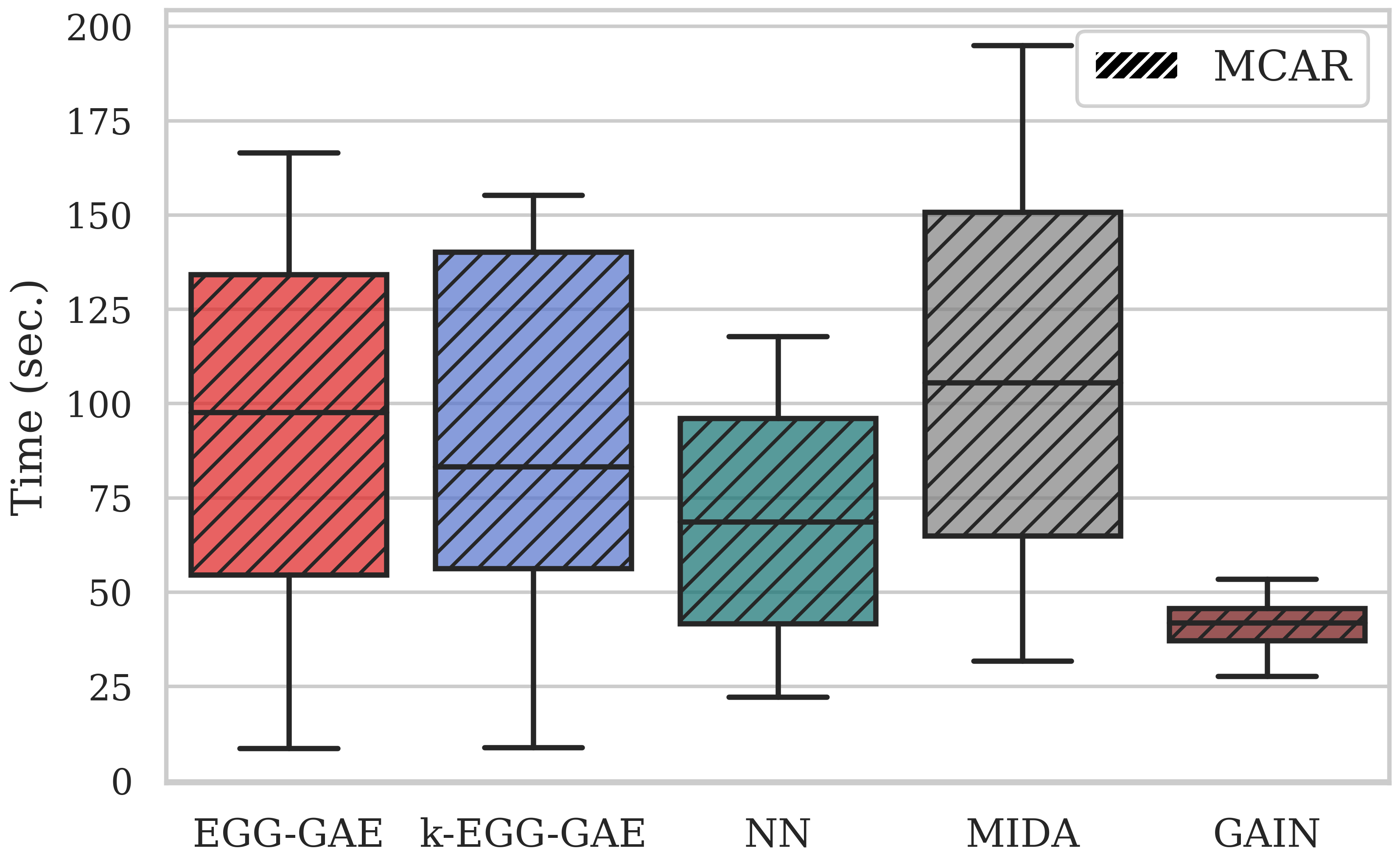
(a) Average training time

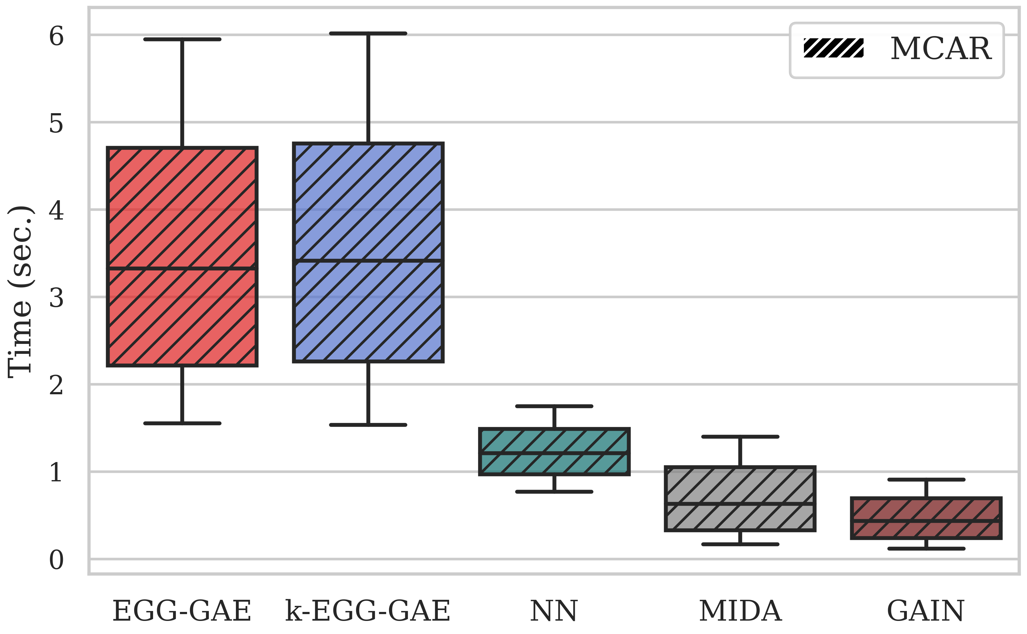
(b) Average inference time

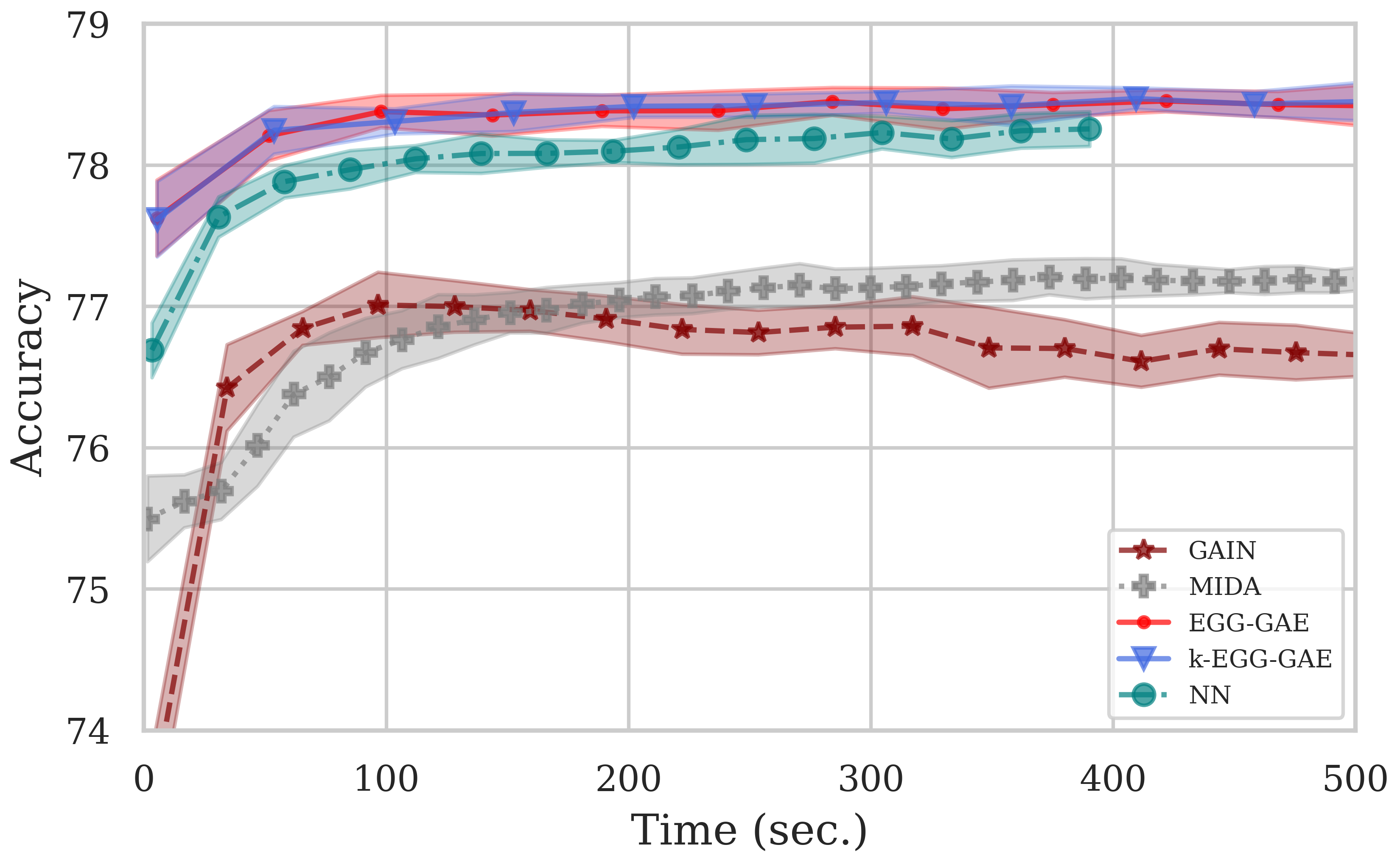
(c) Accuracy over time

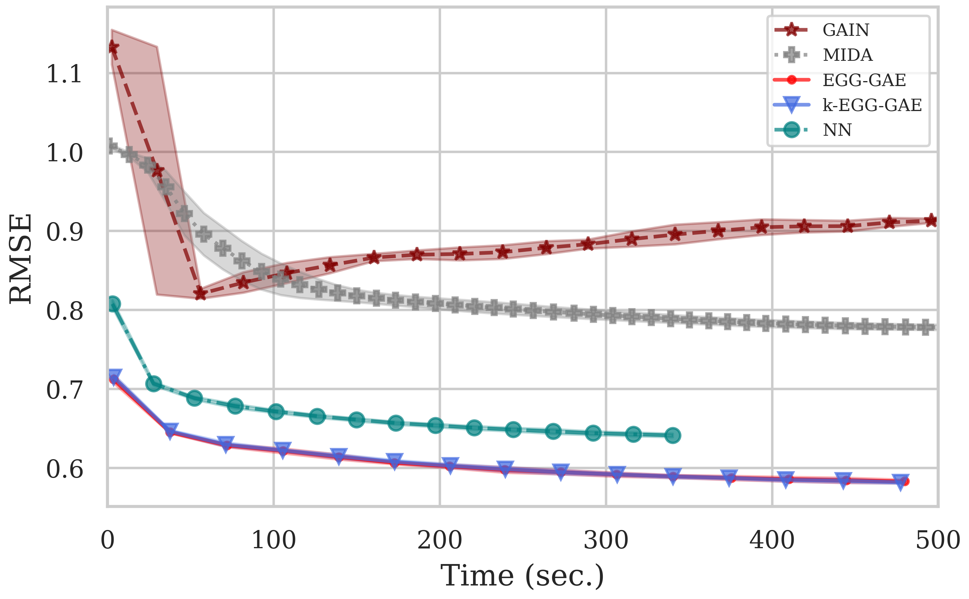
(d) RMSE over time

Figure 5: Average training/inference and performace time comparison for the neural approaches.

6 DISCUSSION AND CONCLUSION

In this paper, we propose a generic framework for handling missing values in tabular data, employing graph deep learning. Particularly, we presented an end-to-end trainable graph autoencoder (EGG-GAE) model for learning the underlying graph representation of tabular data applied to the MDI problem. We performed extensive experiments with real-world datasets (from different fields) and determined that our model outperformed current state-of-the-art algorithms in terms of imputation and downstream task performance. We described several improvements to our model by demonstrating that ensembling improves MDI and dataset task performances; we further introduced novel learnable prototype nodes to encode common data patterns and serve as a generic, reliable subset of nodes for the predicted graphs. Finally, we introduced a regularization method that forces homophily in the learned latent graph representation.

As future works, the proposed EGG-GAE network can be applied to any type of data to introduce a graph topology for, e.g., imputing missing data over images, audio, or other types of high-dimensional data, exploiting the modularity of modern deep learning architectures. In addition, the Euclidean distance calculation can be substituted with a trainable network to construct probabilistic graphs based on a learned metric distance function. The assumption and limitations of the proposed framework are described in supplementary materials, Appendix C.

 

Supplementary Materials for EGG-GAE: scalable graph neural networks for tabular data imputation

 

Appendix A ARCHITECTURAL EXPERIMENTS

We perform architectural experiments over the numerical datasets (reported in Table 1). The results are averaged across five runs and presented as unified average rankings based on end-to-end accuracy, RMSE and MAE. In Section A.1 we analyse the proposed homophily penalization term, evaluate different GNN heads in Sec. A.2. The effect of extra manipulation of the embedding space obtained by the node projector is investigated in Sec. A.3. Examine the impact of varying the number of neighbours sampled per node in the restricted sampling scheme of the $k$-EGG-GAE model in Section A.4.

A.1 Homophily experiment

We argue that boosting $\gamma$ in Eq.13 enhances the sampling scheme of the EGG-GAE model by restricting the sampling of non-homophilic neighbours. We further investigate the influence of the proposed homophily loss adapted to EGG-GAE model. Fig. 6 demonstrates that, on average, using the homophily regularisation term is beneficial. Increasing the regularisation hyperparameter $\gamma$ results in an improved unified solution on average. Although high penalization improves the performance, the variation of EGG-GAE-$5$ indicates that the performance enhancement has plateaued.

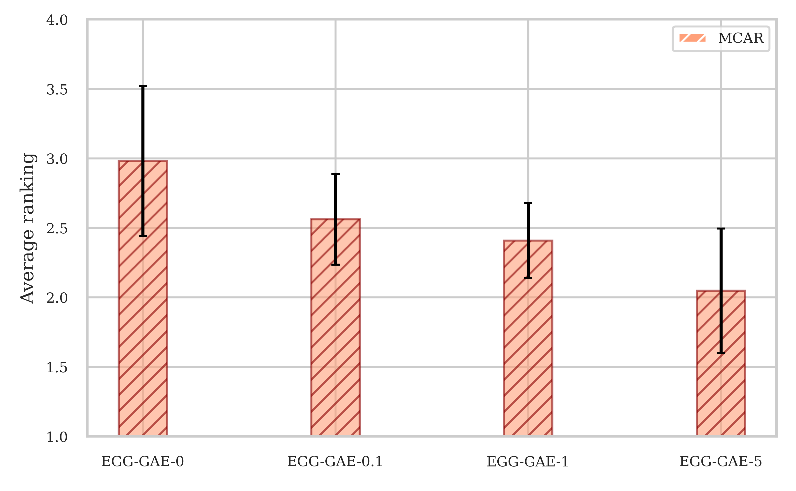
Figure 6: Unified average ranking computed for the MCAR scenario. A value following the model name indicates the regularization hyperparameter $\gamma$.

A.2 Heads experiment

Here we inspect the performance change under different GNNs heads. We explore four heads: GCN (Kipf and Welling,, 2017), EdgeConv (Wang et al.,, 2019), ARMAConv (Bianchi et al.,, 2021) and SGConv (Wu et al.,, 2019). As can be seen in Fig. 7, ARMAConv and EdgeConv on average perform better than GCNConv and SGConv, which achieve roughly the same results, further improving the results from Section 5.1. We hypothesize a potential explanation of ArmaConv and EdgeConv superior performance compared to GCN and SGConv as follows. ArmaConv is more resistant to noise, which increases its resilience to incorrectly sampled connectivity, while EdgeConv intrinsically weights the contribution of each neighbour, providing additional noise resistance and reducing the contribution of not similar examples (which were sampled due to stochasticity) for concrete datum prediction. As a result, an additional filter is applied to the sampled nodes.

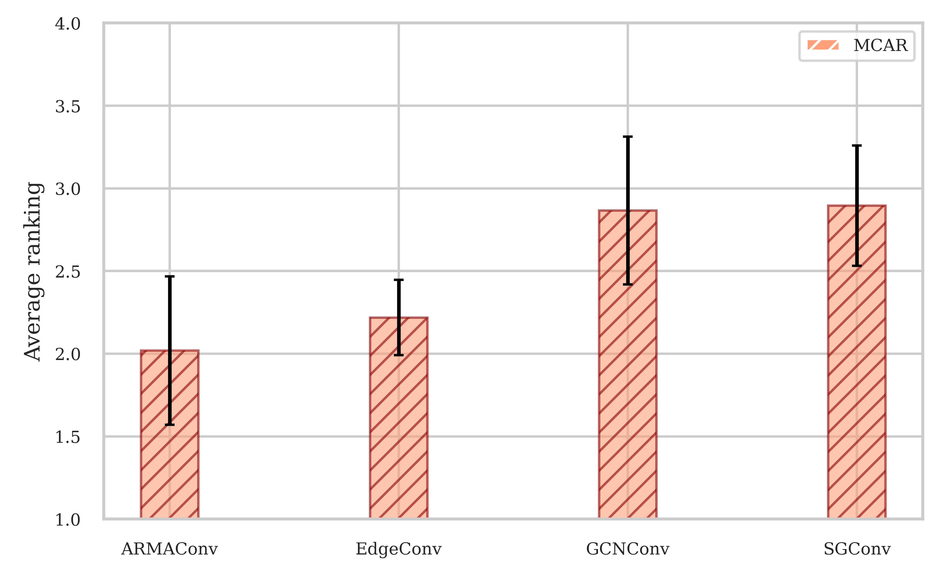
Figure 7: Unified average ranking computed for the MCAR scenario. The model name indicates the head of EGG-GAE model.

A.3 Metric learning experiment

In this part, we investigate the possibility of influencing the embedding space acquired by the node projector. We add additional regularization on the embeddings $\mathrm{H}^{g}_{\mathrm{k}}$ obtained by Eq. 2 using triplet loss Schroff et al., (2015) which is calculated as:

$$\mathcal{L}_{t}=\eta\sum_{i}^{T}{\left[\|{\mathrm{h}}^{a}_{i}-{\mathrm{h}}^{+}_{i}\|^{2}+\|{\mathrm{h}}^{a}_{i}-{\mathrm{h}}^{-}_{i}\|^{2}+\mathrm{m}\right]}$$ (14)

where ${\mathrm{m}}$ is a margin and equal to $0.05$, $\eta$ is a regularization hyperparameter and $\{{\mathrm{h}^{\mathrm{a}}_{i}},{\mathrm{h}^{+}_{i}},{\mathrm{h}^{-}_{i}}\}_{i}^{\mathrm{T}}$ are the triplets formed from embeddings ${\mathrm{H}^{\mathrm{g}}_{\mathrm{k}}}$ forcing the homophily by selecting ${\mathrm{h}^{\mathrm{a}}_{i}}$ and ${\mathrm{h}^{+}_{i}}$ from the same class and ${\mathrm{h}^{-}_{i}}$ from the other. We mine the triplets with distance weighted margin-based approach (Wu et al.,, 2017). Fig. 8 demonstrates applying further regularization on node embedding space can lead to a better solution; nevertheless, the scale parameter $\eta$ has to be carefully chosen, since high values of $\eta$ result in suboptimal solutions.

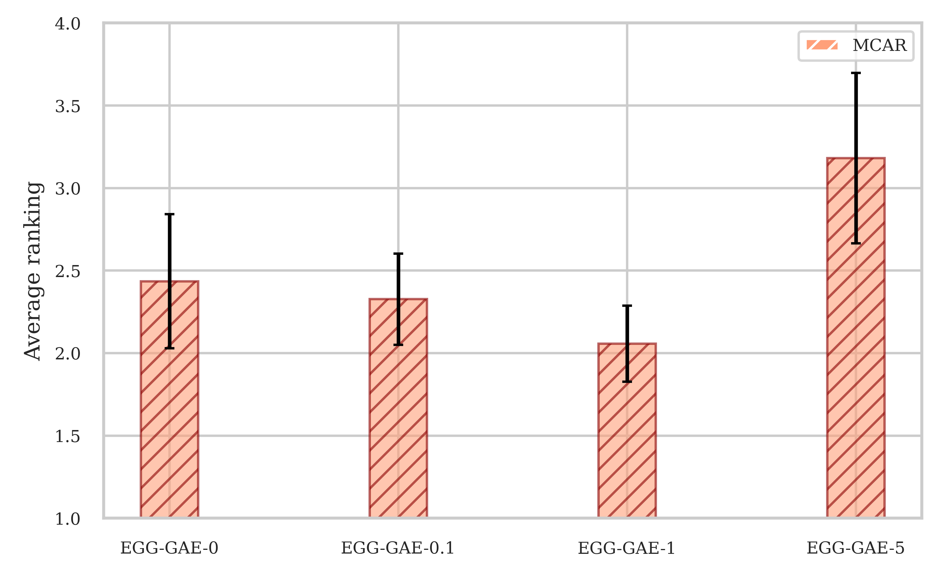
Figure 8: Unified average ranking computed for the MCAR scenario. A value following the model name indicates the regularization hyperparameter $\eta$.

A.4 Restricted sampling

In this section we investigate restrictive sapling procedure by varying the number of sampled neighbours k per node. Figure 9 demonstrates the corresponding experiment, where the model $k$-EGG-GAE-0 is a model which has only self-nodes. Models that rely on the sampled neighbourhood consistently outperform models with only self-nodes in terms of MDI solution and predictive accuracy. Next, we observe that increasing the number $k$ of sampled neighbours improves the performance on average, and that the optimal number of neighbours is $3$. In addition, as the number of sampled neighbours increases, both the average ranking and the variation increase. We hypothesise that this indicates that as the number of sampled neighbours $k$ increases, so does the proportion of noisy neighbours, which degrades performance.

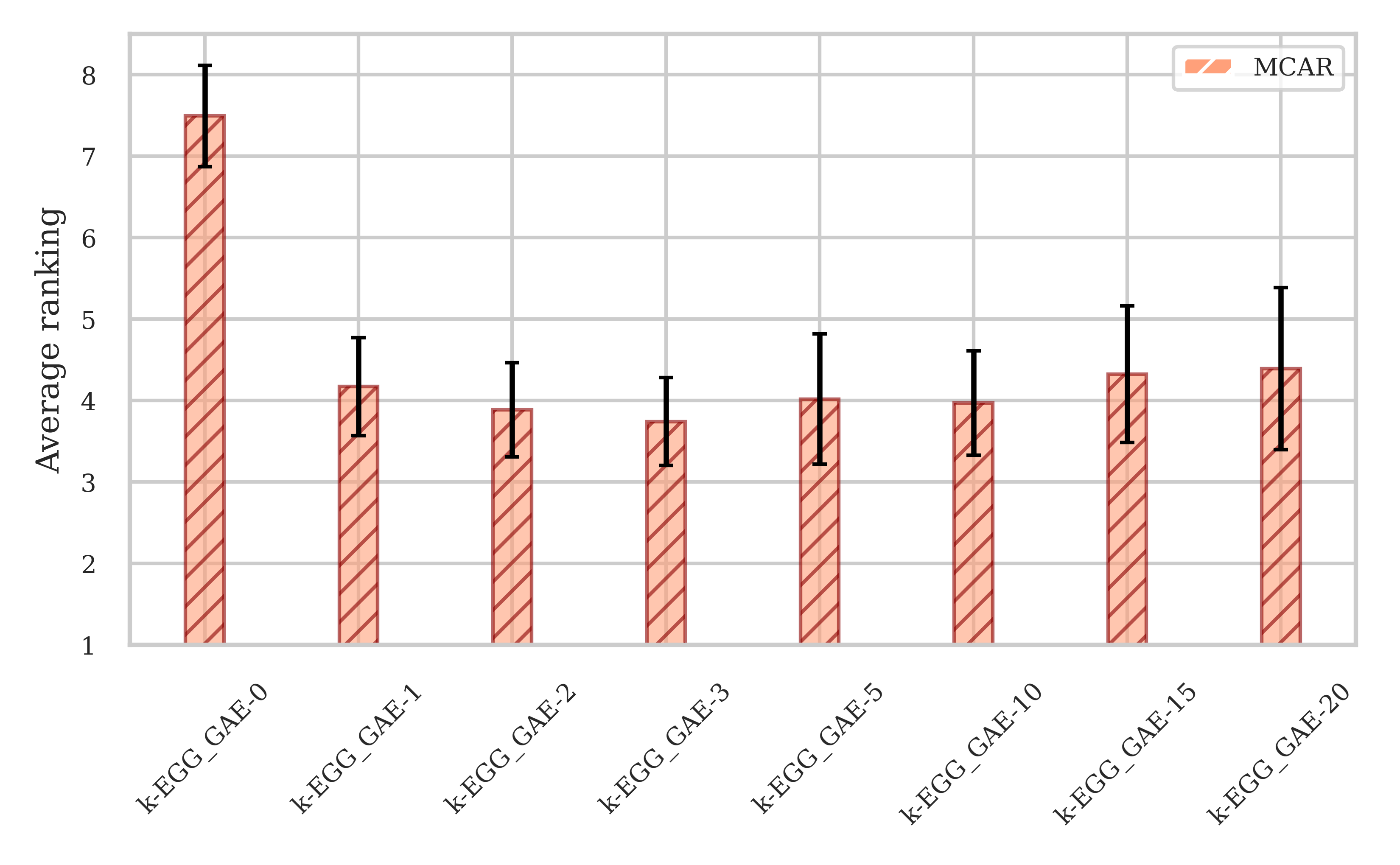
Figure 9: Unified average ranking computed for the MCAR scenario. A value following the model name indicates the number of neighbours sampled per node.

Appendix B IMPUTATION EXPERIMENT

The main set of experiments addresses the imputation reconstruction and predictive performance of the proposed networks in comparison to baseline algorithms utilising the MCAR, MNAR, and MAR mechanisms. The predictive performance of an MDI solution for tabular data is typically measured by classical machine learning (ML) algorithms for a downstream task. To assess post-imputation downstream task performance we employ random forest for all models Breiman, (2001) and provide the findings in Table 2. Tables 3, 4 and 5 display the MDI reconstruction error in terms of RMSE, MAE, and accuracy for numerical and categorical values, respectively, when 20% of values are missing. Due to the fact that the execution time exceeds 24 hours, some GINN results are unavailable and denoted by “-” in the table.

According to Tables 2-5 we can see that for the majority of datasets the proposed EGG-GAE and $k$-EGG-GAE prevail as the best or second best solution in terms of post-imputation predictive performance and MDI solution, regardless of the missingness mechanism. Tables 2 and 5 demonstrates that for categorical data, algorithms inferring similar data points (EGG-GAE, $k$-EGG-GAE, GINN, and KNNI) achieve the best predictive and MDI performance. Regarding MDI performance, the cumulative number of wins of models employing similar datapoints is 23 out of 24 cases. Additionally, it is noticeable in Table 3, that $k$-EGG-GAE model dominates in 50% of cases in total, and 60% cases considering MNAR missigness mechanism. From Table 4, we can see that the machine learning algorithm MF achieves the best result in 10 out of 24 cases, compared to the cumulative win of EGG-GAE and $k$-EGG-GAE models (the cases when the proposed models shares first and second place): in 9 out of 24 instances; however, from the schematic representation (Figure 3(a)), it is evident that $k$-EGG-GAE dominates over the MF algorithm when all performance metrics are considered (predictive and imputation accuracy, RMSE, MAE).

Table 2: Post-imputation downstream task predictive performance in terms of accuracy (Average±Std, averaged over 5 runs) under MCAR, MNAR and MAR assumptions (the case in which $20\%$ of entries are missing). The best results for each dataset are highlighted in bold font, and the second-best result is underlined.

Miss. Dataset type Dataset EGG-GAE k-EGG-GAE NN GINN GAIN MIDA KNNI MICE MF Mean MCAR Numerical Yeast 51.27±0.68 52.02±1.55 49.78±1.19 48.28±0.93 50.07±1.04 50.37±1.37 46.19±0.0 51.12±0.0 50.97±0.68 48.88±0.0 Wireless 95.33±0.58 95.33±0.0 95.0±0.0 91.44±2.34 90.78±1.68 92.11±2.14 91.33±0.0 95.67±0.0 95.0±0.0 89.0±0.0 Abalone 59.86±0.4 59.81±0.28 59.7±0.49 56.51±0.24 58.53±0.32 59.17±0.42 59.17±0.0 60.93±0.0 59.91±0.74 57.1±0.0 Wine quality 50.48±0.14 50.43±0.44 50.43±0.42 49.61±0.28 50.84±0.57 50.11±0.77 50.88±0.0 50.2±0.0 50.34±0.24 49.52±0.0 Page blocks 93.91±0.0 93.75±0.19 93.71±0.07 93.02±0.14 93.95±0.07 93.26±0.07 94.28±0.0 94.03±0.0 94.03±0.12 93.42±0.0 Electrical grid stability 95.69±0.27 95.82±0.2 95.64±0.08 90.87±0.18 93.0±0.0 94.22±0.15 94.07±0.0 94.53±0.0 95.13±0.74 93.0±0.0 SUSY (small) 75.79±0.11 75.73±0.15 75.55±0.15 – 75.02±0.08 75.08±0.12 75.28±0.0 75.35±0.0 75.38±0.16 75.52±0.0 Categorical Car 70.0±0.77 70.38±0.38 69.23±0.67 70.0±0.0 69.87±0.22 69.74±0.22 70.0±0.0 70.38±0.0 70.0±0.0 68.85±0.0 Phishing website 82.59±0.28 82.92±1.86 81.44±0.57 78.0±0.28 81.61±1.24 81.77±0.49 82.27±0.0 79.8±0.0 80.79±0.49 79.8±0.0 Letter 48.03±0.71 47.56±1.1 45.59±0.95 40.63±0.24 42.93±0.29 43.73±0.07 52.63±0.0 46.0±0.0 46.04±0.12 43.23±0.0 Chess 25.32±0.22 25.27±0.65 25.24±0.07 – 26.48±0.07 26.17±0.27 26.35±0.0 25.23±0.0 25.47±0.26 27.06±0.0 Connect 65.92±0.05 65.92±0.03 65.96±0.01 – 65.86±0.01 65.94±0.01 65.96±0.0 66.03±0.0 66.03±0.03 65.86±0.0 Mixed Anuran 92.01±0.37 92.28±0.33 90.12±0.37 85.62±0.89 87.35±0.33 86.27±0.27 91.11±0.0 89.26±0.0 91.54±0.23 85.28±0.0 Adult 81.92±0.31 81.83±0.37 81.4±0.2 – 79.68±0.58 80.02±0.02 79.69±0.0 80.32±0.0 80.85±0.27 80.13±0.0 Default credit card 80.54±0.09 80.53±0.06 80.59±0.09 – 80.26±0.06 80.18±0.04 80.47±0.0 80.51±0.0 80.52±0.05 80.2±0.0 MNAR Numerical Yeast 49.15±0.87 46.37±1.57 46.37±0.87 48.61±0.25 48.07±1.02 48.97±1.16 46.19±0.0 48.88±0.0 48.7±0.68 49.33±0.0 Wireless 93.8±0.45 94.0±0.24 93.47±0.61 93.27±0.55 90.8±1.04 92.2±0.51 92.0±0.0 93.33±0.0 93.2±0.3 90.33±0.0 Abalone 58.09±0.43 58.21±0.6 57.99±0.24 57.45±0.58 57.93±0.93 57.07±0.63 58.21±0.0 59.01±0.0 58.28±0.6 57.74±0.0 Wine quality 52.57±1.05 52.19±0.27 52.14±0.31 50.29±0.4 51.32±0.31 51.51±0.56 51.43±0.0 51.84±0.0 51.7±0.35 50.61±0.0 Page blocks 94.45±0.14 94.57±0.18 94.15±0.24 92.81±0.09 94.42±0.05 94.13±0.1 94.52±0.0 94.52±0.0 94.57±0.33 94.28±0.0 Electrical grid stability 97.07±0.13 97.01±0.13 96.43±0.06 91.75±0.58 94.8±0.0 95.35±0.1 96.07±0.0 96.0±0.0 95.85±0.46 94.8±0.0 SUSY (small) 75.48±0.07 75.53±0.13 75.31±0.07 – 74.2±0.18 74.97±0.18 74.81±0.0 75.59±0.0 75.37±0.11 74.55±0.0 Categorical Car 69.36±0.97 69.62±0.38 69.87±1.11 70.0±0.0 70.9±1.24 70.0±0.0 70.38±0.0 70.38±0.0 70.38±0.38 69.62±0.0 Phishing website 83.91±0.28 82.76±0.49 77.67±1.03 82.76±0.0 81.94±1.03 82.76±0.49 82.27±0.0 79.8±0.0 81.44±1.5 75.86±0.0 Letter 47.43±1.1 47.26±0.51 43.77±0.32 40.57±0.06 42.61±0.51 43.19±0.22 51.8±0.0 47.77±0.0 47.43±1.08 43.17±0.0 Chess 25.99±0.33 26.33±0.21 25.75±0.49 – 26.88±0.03 25.42±1.69 26.42±0.0 26.51±0.0 26.17±0.83 24.04±0.0 Connect 65.88±0.01 65.9±0.06 65.95±0.04 – 66.02±0.03 66.0±0.02 66.0±0.0 66.05±0.0 66.04±0.03 65.89±0.0 Mixed Anuran 91.7±0.35 91.73±0.19 90.74±0.24 89.26±0.83 90.15±0.14 86.64±0.37 91.11±0.0 89.54±0.0 91.42±0.21 85.83±0.0 Adult 81.58±0.63 81.47±0.32 82.01±0.19 – 79.3±0.39 79.63±0.01 79.82±0.0 81.06±0.0 80.41±0.49 80.02±0.0 Default credit card 80.7±0.13 80.73±0.19 80.65±0.05 – 80.58±0.08 80.51±0.07 80.82±0.0 80.49±0.0 80.53±0.06 80.47±0.0 MAR Numerical Yeast 48.97±0.74 49.51±0.68 49.33±1.0 50.49±0.68 48.34±2.14 50.13±1.4 50.22±0.0 48.43±0.0 49.33±1.93 50.67±0.0 Wireless 95.6±0.37 94.87±0.18 94.93±0.64 94.33±1.33 92.07±2.25 94.67±0.82 94.33±0.0 95.0±0.0 95.27±0.37 92.33±0.0 Abalone 58.66±0.57 58.37±0.37 58.18±0.44 57.26±0.52 58.15±0.79 57.58±0.44 60.13±0.0 58.37±0.0 58.56±0.73 56.78±0.0 Wine quality 52.79±0.54 52.6±0.61 52.76±0.31 49.55±0.47 50.1±0.56 51.51±0.34 52.79±0.0 51.7±0.0 52.35±0.06 51.29±0.0 Page blocks 94.52±0.19 94.74±0.16 94.45±0.11 93.54±0.17 94.47±0.33 94.2±0.07 94.64±0.0 94.52±0.0 94.74±0.1 93.91±0.0 Electrical grid stability 97.49±0.22 97.56±0.12 96.84±0.18 93.59±0.48 94.8±0.0 95.36±0.1 96.47±0.0 96.53±0.0 96.08±0.23 94.8±0.0 SUSY (small) 75.64±0.07 75.58±0.08 75.46±0.12 – 75.17±0.18 75.31±0.1 75.24±0.0 75.79±0.0 75.6±0.11 75.97±0.0 Categorical Car 69.46±0.64 70.0±0.72 69.85±0.34 70.77±0.0 70.08±0.63 70.0±0.0 70.77±0.0 70.38±0.0 70.54±0.34 68.46±0.0 Phishing website 83.25±0.49 83.58±0.28 80.79±1.71 82.27±0.0 81.28±0.85 81.28±0.0 85.71±0.0 80.3±0.0 82.76±1.3 77.83±0.0 Letter 48.77±1.05 49.31±0.41 46.12±1.17 42.41±0.02 38.0±0.71 45.12±0.43 52.13±0.0 47.97±0.0 46.61±0.91 45.07±0.0 Chess 26.46±0.59 26.05±0.84 25.89±0.85 – 27.04±0.06 25.02±0.75 26.94±0.0 27.25±0.0 27.13±0.51 23.78±0.0 Connect 66.05±0.03 66.05±0.05 66.0±0.02 – 66.0±0.06 66.0±0.01 66.09±0.0 66.08±0.0 66.07±0.02 65.92±0.0 Mixed Anuran 91.82±0.23 91.91±0.77 90.96±0.23 89.69±0.27 88.8±0.24 86.94±0.19 91.11±0.0 89.54±0.0 91.94±0.19 87.78±0.0 Adult 81.27±0.21 81.36±0.5 81.67±0.17 – 79.1±0.81 79.64±0.04 80.91±0.0 80.32±0.0 81.22±0.27 80.13±0.0 Default credit card 80.64±0.14 80.61±0.09 80.81±0.08 – 80.64±0.11 80.67±0.07 80.64±0.0 80.67±0.0 80.56±0.04 80.6±0.0

Table 3: Imputation performance in terms of RMSE (Average±Std, averaged over 5 runs) under MCAR, MNAR and MAR assumptions (the case in which $20\%$ of entries are missing). The best results for each dataset are highlighted in bold font, and the second-best result is underlined.

Miss. Data type Dataset EGG-GAE k-EGG-GAE NN GINN GAIN MIDA KNNI MICE MF Mean MCAR Numerical Yeast 0.9343±0.0069 0.9271±0.0099 0.9431±0.0063 1.0749±0.0401 1.061±0.0052 0.9825±0.0031 1.014±0.0 0.9315±0.0 0.9222±0.0259 0.9987±0.0 Wireless 0.6082±0.001 0.6067±0.0102 0.645±0.0091 1.078±0.007 0.8865±0.1909 0.8097±0.0176 0.7341±0.0 0.6351±0.0 0.6425±0.0156 0.9851±0.0 Abalone 0.3982±0.0036 0.3925±0.0025 0.4586±0.0046 1.5066±0.2678 0.6314±0.0608 0.5183±0.0018 0.4931±0.0 0.4051±0.0 0.3747±0.0063 0.9781±0.0 Wine quality 0.803±0.0047 0.8006±0.0032 0.8398±0.011 1.3678±0.055 0.9491±0.0066 0.9125±0.0065 0.8658±0.0 0.8268±0.0 0.8204±0.0034 1.0314±0.0 Page blocks 0.6211±0.0048 0.6218±0.0056 0.6673±0.0084 1.1888±0.0113 0.9939±0.0047 0.8385±0.0059 0.6813±0.0 0.7527±0.0 0.6056±0.0273 1.0947±0.0 Electrical grid stability 0.8587±0.0013 0.8588±0.0028 0.8862±0.0006 1.2907±0.0247 0.9902±0.0253 0.9768±0.0026 0.9966±0.0 0.9018±0.0 0.9112±0.0047 1.0193±0.0 SUSY (small) 0.5781±0.0014 0.5772±0.0038 0.6542±0.003 – 0.881±0.0468 0.777±0.0029 0.7078±0.0 0.666±0.0 0.638±0.0019 1.0195±0.0 Mixed Anuran 0.4978±0.0104 0.4966±0.0037 0.5878±0.0032 1.0423±0.0112 0.8446±0.0169 0.9867±0.0275 0.4808±0.0 0.5893±0.0 0.5431±0.0087 1.0405±0.0 Adult 0.8568±0.0027 0.8538±0.0032 0.8746±0.0004 – 0.9983±0.0063 0.9928±0.0014 0.9321±0.0 0.9574±0.0 0.9132±0.0065 0.9999±0.0 Default credit card 0.6309±0.0222 0.6224±0.0116 0.7086±0.0031 – 1.0293±0.2887 0.9621±0.01 0.7338±0.0 0.6802±0.0 0.641±0.0142 1.0121±0.0 MNAR Numerical Yeast 0.7787±0.0087 0.7739±0.0083 0.7739±0.0006 0.9819±0.0332 0.9562±0.0206 0.7934±0.0022 0.8633±0.0 0.7396±0.0 0.875±0.0282 0.8295±0.0 Wireless 0.6864±0.008 0.6806±0.0023 0.717±0.0061 1.2162±0.0199 0.9905±0.1485 0.8836±0.0274 0.7612±0.0 0.7016±0.0 0.7213±0.0102 1.0959±0.0 Abalone 0.4032±0.0045 0.4072±0.0086 0.5075±0.0095 1.3258±0.0264 0.6234±0.0682 0.5521±0.0012 0.4503±0.0 0.3854±0.0 0.3836±0.0049 1.116±0.0 Wine quality 0.7693±0.0161 0.7581±0.0051 0.7761±0.0034 1.1364±0.0258 0.9264±0.0017 0.853±0.0055 0.8137±0.0 0.8722±0.0 0.7786±0.0071 0.9738±0.0 Page blocks 0.6971±0.0149 0.6842±0.0053 0.7284±0.003 1.373±0.0246 1.3086±0.1741 0.9244±0.0056 0.7626±0.0 0.8433±0.0 0.7396±0.0855 1.1922±0.0 Electrical grid stability 0.8556±0.0017 0.8543±0.001 0.8835±0.0007 1.403±0.0207 1.0091±0.0366 0.9646±0.0048 1.0049±0.0 0.8952±0.0 0.9196±0.006 1.0114±0.0 SUSY (small) 0.5785±0.006 0.5752±0.0028 0.6589±0.0026 – 1.0478±0.0462 0.7746±0.0031 0.7022±0.0 0.6726±0.0 0.6357±0.0042 1.0178±0.0 Mixed Anuran 0.4274±0.0081 0.4335±0.0052 0.5214±0.003 1.0255±0.0124 0.8864±0.0626 1.0009±0.0098 0.4092±0.0 0.5027±0.0 0.4878±0.0048 1.0541±0.0 Adult 0.8643±0.0057 0.8639±0.0043 0.883±0.0019 – 1.0271±0.0023 1.0036±0.0003 0.9693±0.0 0.9772±0.0 0.9665±0.0379 1.0107±0.0 Default credit card 0.6949±0.0038 0.6953±0.001 0.7409±0.0016 – 1.366±0.1709 1.0112±0.0114 0.7515±0.0 0.8555±0.0 0.7063±0.0159 1.0731±0.0 MAR Numerical Yeast 0.8196±0.019 0.8163±0.0128 0.8059±0.0057 0.8575±0.0178 1.0849±0.0917 0.8085±0.0019 0.9018±0.0 0.7909±0.0 0.8748±0.0346 0.8503±0.0 Wireless 0.6408±0.0104 0.635±0.0026 0.6805±0.0036 1.2775±0.0159 1.0775±0.1336 0.8625±0.0203 0.644±0.0 0.6748±0.0 0.6772±0.0153 1.125±0.0 Abalone 0.3913±0.0038 0.4003±0.0057 0.4984±0.0124 1.3368±0.028 0.7047±0.1387 0.5436±0.0043 0.4088±0.0 0.3837±0.0 0.3851±0.013 1.1543±0.0 Wine quality 0.7018±0.0073 0.6949±0.0034 0.7079±0.0033 1.1996±0.0635 1.2254±0.0999 0.8075±0.0065 0.7125±0.0 0.7295±0.0 0.6994±0.0018 0.9547±0.0 Page blocks 0.68±0.0037 0.6718±0.0105 0.7535±0.0082 1.386±0.0058 1.6437±0.7462 0.9527±0.0069 0.667±0.0 0.8807±0.0 0.6744±0.0449 1.2318±0.0 Electrical grid stability 0.8141±0.0009 0.813±0.0026 0.8483±0.0007 1.3966±0.0251 1.0399±0.0344 0.9533±0.0069 0.96±0.0 0.8318±0.0 0.8875±0.0021 1.0124±0.0 SUSY (small) 0.5213±0.0026 0.5222±0.0023 0.6206±0.005 – 1.1357±0.0857 0.7572±0.0033 0.6158±0.0 0.6116±0.0 0.602±0.0016 1.0217±0.0 Mixed Anuran 0.4363±0.0023 0.4401±0.006 0.5353±0.0048 1.0484±0.0188 1.7316±0.1103 1.0338±0.0154 0.4201±0.0 0.5038±0.0 0.514±0.0012 1.0968±0.0 Adult 0.8333±0.0027 0.8323±0.0017 0.8672±0.0015 – 1.514±0.5263 1.0078±0.0027 0.8603±0.0 0.9779±0.0 0.8501±0.0059 1.012±0.0 Default credit card 0.7012±0.0015 0.6983±0.0065 0.7514±0.0033 – 1.2989±0.2358 0.9903±0.0306 0.7488±0.0 0.7081±0.0 0.6974±0.025 1.0719±0.0

Table 4: Imputation performance in terms of MAE (Average±Std, averaged over 5 runs) under MCAR, MNAR and MAR assumptions (the case in which $20\%$ of entries are missing). The best results for each dataset are highlighted in bold font, and the second-best result is underlined.

Miss. Data type Dataset EGG-GAE k-EGG-GAE NN GINN GAIN MIDA KNNI MICE MF Mean MCAR Numerical Yeast 0.5299±0.0071 0.5256±0.0104 0.5459±0.0083 0.5957±0.0335 0.6128±0.0557 0.5587±0.0038 0.5728±0.0 0.5258±0.0 0.5279±0.0098 0.5217±0.0 Wireless 0.4469±0.0022 0.445±0.0064 0.4884±0.0071 0.8302±0.0046 0.7233±0.1179 0.6142±0.0213 0.5467±0.0 0.4737±0.0 0.4593±0.0116 0.7771±0.0 Abalone 0.2673±0.0064 0.2577±0.002 0.3396±0.0071 1.0507±0.1161 0.563±0.0938 0.3687±0.0013 0.3004±0.0 0.2414±0.0 0.2306±0.0013 0.7755±0.0 Wine quality 0.5596±0.0091 0.5597±0.005 0.5849±0.0076 1.086±0.0488 0.6939±0.0046 0.6476±0.0067 0.6014±0.0 0.5699±0.0 0.565±0.0027 0.7499±0.0 Page blocks 0.3204±0.0064 0.3181±0.0071 0.3675±0.0074 0.7765±0.01 0.6148±0.0043 0.4683±0.0032 0.2902±0.0 0.4091±0.0 0.2711±0.009 0.605±0.0 Electrical grid stability 0.7148±0.0011 0.713±0.0033 0.7444±0.0004 1.059±0.0175 0.8501±0.0276 0.8328±0.0008 0.8297±0.0 0.6791±0.0 0.7427±0.0042 0.8809±0.0 SUSY (small) 0.3776±0.0014 0.3798±0.005 0.4484±0.003 – 0.6804±0.0275 0.5487±0.0032 0.4436±0.0 0.4469±0.0 0.4152±0.0015 0.7453±0.0 Mixed Anuran 0.2905±0.0036 0.2898±0.0041 0.3643±0.0026 0.7337±0.0097 0.6273±0.0079 0.7068±0.0383 0.2418±0.0 0.3317±0.0 0.3173±0.0024 0.7442±0.0 Adult 0.4774±0.0045 0.4775±0.0058 0.5091±0.0033 – 0.6029±0.0048 0.5867±0.0022 0.5344±0.0 0.6024±0.0 0.4919±0.005 0.5391±0.0 Default credit card 0.2597±0.0136 0.2559±0.0101 0.3104±0.0028 – 0.4818±0.0399 0.5039±0.0154 0.2345±0.0 0.2505±0.0 0.209±0.002 0.4585±0.0 MNAR Numerical Yeast 0.5701±0.013 0.5624±0.0079 0.5587±0.005 0.6436±0.0216 0.6682±0.0521 0.5415±0.0028 0.5794±0.0 0.5305±0.0 0.5891±0.0159 0.5261±0.0 Wireless 0.5088±0.0074 0.5052±0.0026 0.5384±0.0061 0.9311±0.0199 0.8447±0.095 0.6793±0.0225 0.5678±0.0 0.5354±0.0 0.5075±0.0085 0.8922±0.0 Abalone 0.2797±0.0043 0.2891±0.0075 0.3657±0.0039 1.0653±0.0251 0.6671±0.076 0.3918±0.0019 0.2913±0.0 0.2331±0.0 0.2426±0.0042 0.8826±0.0 Wine quality 0.5534±0.0055 0.5521±0.0117 0.5678±0.0038 0.8638±0.0222 0.7241±0.0198 0.6385±0.0039 0.5883±0.0 0.6033±0.0 0.5521±0.0039 0.7288±0.0 Page blocks 0.3463±0.0051 0.3422±0.0072 0.3912±0.0049 0.8623±0.0159 0.6402±0.0183 0.5015±0.0049 0.3353±0.0 0.4598±0.0 0.292±0.0108 0.675±0.0 Electrical grid stability 0.7045±0.002 0.7028±0.0009 0.7384±0.0011 1.1405±0.0153 0.8499±0.0252 0.8244±0.0053 0.8282±0.0 0.6789±0.0 0.7474±0.005 0.8736±0.0 SUSY (small) 0.3739±0.0028 0.3734±0.0011 0.4472±0.0023 – 0.7795±0.0224 0.5495±0.0037 0.4404±0.0 0.4475±0.0 0.4102±0.002 0.7438±0.0 Mixed Anuran 0.2876±0.0059 0.2899±0.006 0.3628±0.0018 0.7899±0.0023 0.6611±0.0784 0.7679±0.01 0.2501±0.0 0.3324±0.0 0.3172±0.0025 0.7911±0.0 Adult 0.4815±0.0071 0.4797±0.01 0.5055±0.001 – 0.6669±0.0674 0.5942±0.0071 0.5597±0.0 0.6143±0.0 0.5213±0.0136 0.5427±0.0 Default credit card 0.2538±0.0058 0.2575±0.0008 0.2916±0.0036 – 0.6308±0.0385 0.5052±0.0148 0.2308±0.0 0.3219±0.0 0.2183±0.0033 0.47±0.0 MAR Numerical Yeast 0.6059±0.0173 0.604±0.0119 0.5829±0.01 0.5925±0.0175 1.0058±0.2793 0.5673±0.004 0.6328±0.0 0.5699±0.0 0.6061±0.0165 0.5566±0.0 Wireless 0.4746±0.0074 0.4743±0.0035 0.511±0.0037 0.9639±0.0139 0.929±0.0459 0.6702±0.0171 0.4759±0.0 0.5158±0.0 0.4711±0.0091 0.9157±0.0 Abalone 0.2921±0.0132 0.3001±0.0069 0.3711±0.0066 1.0879±0.0348 0.652±0.0891 0.3973±0.004 0.2709±0.0 0.2409±0.0 0.2514±0.0039 0.9208±0.0 Wine quality 0.5113±0.0096 0.4977±0.0075 0.5208±0.0022 0.9236±0.0389 0.9259±0.0472 0.6061±0.0076 0.5052±0.0 0.5137±0.0 0.497±0.0059 0.7183±0.0 Page blocks 0.3036±0.0092 0.2947±0.0068 0.3459±0.0025 0.8488±0.0044 0.8011±0.1234 0.4557±0.0075 0.2212±0.0 0.422±0.0 0.2519±0.013 0.639±0.0 Electrical grid stability 0.6574±0.0012 0.6568±0.0019 0.7018±0.0023 1.1384±0.0174 0.898±0.0155 0.8115±0.0053 0.7875±0.0 0.6158±0.0 0.7153±0.0082 0.873±0.0 SUSY (small) 0.3274±0.0014 0.3243±0.0006 0.4095±0.0049 – 0.8485±0.0269 0.5244±0.0028 0.3751±0.0 0.3941±0.0 0.3793±0.0021 0.7507±0.0 Mixed Anuran 0.2938±0.0034 0.293±0.0024 0.3707±0.0033 0.8179±0.0084 1.3936±0.0946 0.8071±0.0185 0.2637±0.0 0.3414±0.0 0.3409±0.0032 0.8439±0.0 Adult 0.4113±0.0096 0.4122±0.0104 0.4616±0.001 – 0.7908±0.2128 0.5886±0.0071 0.4591±0.0 0.6054±0.0 0.3816±0.003 0.5429±0.0 Default credit card 0.2301±0.0097 0.225±0.0071 0.2649±0.0013 – 0.8806±0.0318 0.4543±0.0384 0.1925±0.0 0.2108±0.0 0.1794±0.0029 0.4238±0.0

Table 5: Imputation performance in terms of Accuracy of reconstructed categorical variables (Average±Std, averaged over 5 runs) under MCAR, MNAR and MAR assumptions (the case in which $20\%$ of entries are missing). The best results for each dataset are highlighted in bold font, and the second-best result is underlined.

Miss. Dataset type Dataset EGG-GAE k-EGG-GAE NN GINN GAIN MIDA KNNI MICE MF Mean MCAR Categorical car 26.6±1.95 22.65±1.03 26.92±1.28 23.08±0.55 30.98±0.49 32.05±1.47 26.28±0.0 27.24±0.0 29.28±1.03 33.33±0.0 phishing website 60.64±1.56 61.19±0.57 57.63±3.47 51.69±0.88 46.21±4.19 41.82±1.11 48.49±0.0 49.59±0.0 49.13±2.8 49.04±0.0 letter 41.1±0.61 40.88±0.35 30.12±0.73 18.2±0.01 22.98±0.95 24.23±0.68 45.75±0.0 26.97±0.0 31.49±0.57 24.52±0.0 chess 23.27±0.21 23.83±0.62 23.58±0.41 20.54±0.03 19.38±0.27 19.16±0.22 20.2±0.0 22.06±0.0 20.57±0.42 23.68±0.0 connect 88.86±0.13 88.9±0.05 86.67±0.14 – 77.97±3.76 83.82±0.03 82.75±0.0 83.8±0.0 84.44±0.35 81.49±0.0 Mixed anuran 82.98±0.84 83.23±0.48 68.73±2.0 40.36±0.0 31.37±0.35 23.64±12.18 83.28±0.0 40.96±0.0 67.47±5.39 41.27±0.0 Adult 72.64±0.54 72.58±0.43 69.18±0.23 – 32.61±2.41 34.54±1.81 42.36±0.0 19.64±0.0 33.39±0.31 55.43±0.0 default credit card 67.82±0.18 68.08±0.37 65.92±0.19 – 48.98±0.2 44.85±9.16 58.31±0.0 46.12±0.0 50.86±2.67 48.89±0.0 MNAR Categorical car 23.82±0.64 23.52±2.77 24.44±3.25 32.62±0.17 30.16±0.94 29.45±0.0 25.46±0.0 29.75±0.0 26.58±2.09 28.83±0.0 phishing website 61.46±0.72 60.8±0.49 55.3±1.85 52.65±0.16 45.74±3.12 42.33±0.75 48.01±0.0 46.31±0.0 46.59±1.24 53.98±0.0 letter 41.67±0.45 41.03±0.33 30.85±0.48 18.18±0.01 22.33±1.92 24.18±0.55 46.01±0.0 26.51±0.0 32.2±0.58 24.95±0.0 chess 22.54±0.45 22.35±0.19 22.2±0.72 – 18.67±0.1 18.36±0.08 18.65±0.0 19.76±0.0 19.57±0.71 21.45±0.0 connect 88.85±0.23 88.92±0.04 86.75±0.1 – 80.55±4.75 84.1±0.03 83.09±0.0 84.05±0.0 83.91±0.06 81.86±0.0 Mixed anuran 84.01±0.77 84.74±0.32 71.41±1.53 62.66±0.0 28.91±2.56 15.31±7.17 85.62±0.0 43.44±0.0 71.62±0.24 45.78±0.0 Adult 73.76±0.53 73.95±0.43 70.8±0.19 – 32.5±3.64 37.14±1.11 36.47±0.0 22.9±0.0 36.58±1.53 58.14±0.0 default credit card 66.79±0.35 66.38±0.15 64.9±0.26 – 42.42±1.49 44.54±9.2 56.47±0.0 42.78±0.0 52.02±2.62 48.51±0.0 MAR Categorical car 23.9±2.05 23.61±2.37 24.33±3.62 33.07±0.32 31.77±1.6 28.88±0.0 25.27±0.0 29.6±0.0 28.45±3.1 29.24±0.0 phishing website 63.47±0.94 62.88±1.95 60.05±1.95 53.07±0.2 45.86±0.73 36.17±0.0 51.77±0.0 45.74±0.0 43.03±1.14 54.61±0.0 letter 44.03±0.63 43.69±0.05 32.65±0.65 20.95±0.01 18.96±0.8 24.38±0.39 52.2±0.0 28.19±0.0 34.99±0.43 26.68±0.0 chess 17.84±0.55 17.62±0.09 17.57±0.59 – 16.59±0.21 16.23±0.39 15.71±0.0 16.67±0.0 16.14±0.49 17.26±0.0 connect 91.58±0.27 91.57±0.23 89.24±0.16 – 83.63±3.84 87.2±0.06 86.38±0.0 87.25±0.0 87.87±0.13 84.45±0.0 Mixed anuran 77.51±0.36 78.62±1.33 62.0±2.03 54.0±0.14 34.68±2.11 6.33±0.9 80.76±0.0 30.64±0.0 59.86±1.33 41.81±0.0 Adult 73.83±0.62 73.13±0.34 69.57±0.13 – 21.24±7.07 29.84±2.02 38.97±0.0 20.67±0.0 37.34±1.76 56.69±0.0 default credit card 62.44±0.08 62.48±0.33 60.97±0.41 – 36.67±2.93 43.98±8.64 53.97±0.0 43.91±0.0 51.22±2.8 46.41±0.0

Appendix C ASSUMPTIONS AND LIMITATIONS

1) The pairwise calculation in the sampling procedure of the EGG block requires $n^{2}$ operations, so increasing the batch size results in a quadratic increase in training/inference time. In addition, we believe that the procedure could generally be replaced with a learnable block. In fact, we believe that the sampling process should be iterable, such that the first iteration provides an initial approximation of the neighbourhood and subsequent iterations eliminate noisy neighbours.

2) In the paper we rely on a pretty simple graph construction approach: from the sampled batch $\mathrm{X}$ we construct for each node its neighbourhood and pass the obtained graph through a GNN head. There are a number of modifications that will allow to obtain better gradients, resulting in a better solution. For example, we can extract $\mathrm{b}$ combinations of $\mathrm{m}$ rows from the obtained matrix $\mathrm{P}$ (with/without repetitions), and then carry out the subsequent operations described in Section 4 without modification. Such modification will allows us to obtain multiple predictions for the same data point in a single pass, resulting in a theoretically better gradient.

References

- Acuna and Rodriguez, (2004) Acuna, E. and Rodriguez, C. (2004). The treatment of missing values and its effect on classifier accuracy. In Classification, clustering, and data mining applications, pages 639–647. Springer.
- Azur et al., (2011) Azur, M. J., Stuart, E. A., Frangakis, C., and Leaf, P. J. (2011). Multiple imputation by chained equations: what is it and how does it work? International journal of methods in psychiatric research, 20(1):40–49.
- Bengio and Gingras, (1995) Bengio, Y. and Gingras, F. (1995). Recurrent neural networks for missing or asynchronous data. Advances in neural information processing systems, 8.
- Bertsimas et al., (2017) Bertsimas, D., Pawlowski, C., and Zhuo, Y. D. (2017). From predictive methods to missing data imputation: an optimization approach. J. Mach. Learn. Res., 18(1):7133–7171.
- Bianchi et al., (2021) Bianchi, F. M., Grattarola, D., Livi, L., and Alippi, C. (2021). Graph neural networks with convolutional arma filters. IEEE Transactions on Pattern Analysis and Machine Intelligence.
- Breiman, (2001) Breiman, L. (2001). Random forests. Machine learning, 45(1):5–32.
- Chen et al., (2020) Chen, X., Chen, S., Yao, J., Zheng, H., Zhang, Y., and Tsang, I. W. (2020). Learning on attribute-missing graphs. IEEE transactions on pattern analysis and machine intelligence.
- Cong et al., (2020) Cong, W., Forsati, R., Kandemir, M., and Mahdavi, M. (2020). Minimal variance sampling with provable guarantees for fast training of graph neural networks. In 26th ACM SIGKDD International Conference on Knowledge Discovery & Data Mining, pages 1393–1403.
- Cosmo et al., (2020) Cosmo, L., Kazi, A., Ahmadi, S.-A., Navab, N., and Bronstein, M. (2020). Latent-graph learning for disease prediction. In International Conference on Medical Image Computing and Computer-Assisted Intervention, pages 643–653. Springer.
- Farhangfar et al., (2007) Farhangfar, A., Kurgan, L. A., and Pedrycz, W. (2007). A novel framework for imputation of missing values in databases. IEEE Transactions on Systems, Man, and Cybernetics-Part A: Systems and Humans, 37(5):692–709.
- Gilmer et al., (2017) Gilmer, J., Schoenholz, S. S., Riley, P. F., Vinyals, O., and Dahl, G. E. (2017). Neural message passing for quantum chemistry. In International Conference on Machine Learning (ICML), pages 1263–1272. PMLR.
- Gondara and Wang, (2018) Gondara, L. and Wang, K. (2018). Mida: Multiple imputation using denoising autoencoders. In Pacific-Asia conference on knowledge discovery and data mining, pages 260–272. Springer.
- Hamilton et al., (2017) Hamilton, W., Ying, Z., and Leskovec, J. (2017). Inductive representation learning on large graphs. Advances in neural information processing systems, 30.
- Jang et al., (2016) Jang, E., Gu, S., and Poole, B. (2016). Categorical reparameterization with gumbel-softmax. arXiv preprint arXiv:1611.01144.
- Jiang and Zhang, (2020) Jiang, B. and Zhang, Z. (2020). Incomplete graph representation and learning via partial graph neural networks. arXiv preprint arXiv:2003.10130.
- Kazi et al., (2022) Kazi, A., Cosmo, L., Ahmadi, S.-A., Navab, N., and Bronstein, M. (2022). Differentiable graph module (dgm) for graph convolutional networks. IEEE Transactions on Pattern Analysis and Machine Intelligence.
- Kipf and Welling, (2017) Kipf, T. N. and Welling, M. (2017). Semi-supervised classification with graph convolutional networks. In International Conference on Learning Representations (ICLR).
- Kool et al., (2019) Kool, W., Van Hoof, H., and Welling, M. (2019). Stochastic beams and where to find them: The gumbel-top-k trick for sampling sequences without replacement. In International Conference on Machine Learning, pages 3499–3508. PMLR.
- Kreindler and Lumsden, (2006) Kreindler, D. M. and Lumsden, C. J. (2006). The effects of the irregular sample and missing data in time series analysis. Nonlinear dynamics, psychology, and life sciences.
- Lakshminarayan et al., (1996) Lakshminarayan, K., Harp, S. A., Goldman, R. P., Samad, T., et al. (1996). Imputation of missing data using machine learning techniques. In KDD, volume 96.
- Little and Rubin, (2019) Little, R. J. and Rubin, D. B. (2019). Statistical analysis with missing data, volume 793. John Wiley & Sons.
- Mackinnon, (2010) Mackinnon, A. (2010). The use and reporting of multiple imputation in medical research–a review. Journal of internal medicine, 268(6):586–593.
- Miao et al., (2022) Miao, X., Wu, Y., Chen, L., Gao, Y., and Yin, J. (2022). An experimental survey of missing data imputation algorithms. IEEE Transactions on Knowledge and Data Engineering.
- Muzellec et al., (2020) Muzellec, B., Josse, J., Boyer, C., and Cuturi, M. (2020). Missing data imputation using optimal transport. In International Conference on Machine Learning, pages 7130–7140. PMLR.
- Narang et al., (2013) Narang, S. K., Gadde, A., and Ortega, A. (2013). Signal processing techniques for interpolation in graph structured data. In 2013 IEEE International Conference on Acoustics, Speech and Signal Processing, pages 5445–5449. IEEE.
- Nazabal et al., (2020) Nazabal, A., Olmos, P. M., Ghahramani, Z., and Valera, I. (2020). Handling incomplete heterogeneous data using vaes. Pattern Recognition, 107:107501.
- Rossi et al., (2021) Rossi, E., Kenlay, H., Gorinova, M. I., Chamberlain, B. P., Dong, X., and Bronstein, M. (2021). On the unreasonable effectiveness of feature propagation in learning on graphs with missing node features. arXiv preprint arXiv:2111.12128.
- Rubin, (1976) Rubin, D. B. (1976). Inference and missing data. Biometrika, 63(3):581–592.
- Schroff et al., (2015) Schroff, F., Kalenichenko, D., and Philbin, J. (2015). Facenet: A unified embedding for face recognition and clustering. In Proceedings of the IEEE conference on computer vision and pattern recognition, pages 815–823.
- Śmieja et al., (2018) Śmieja, M., Struski, Ł., Tabor, J., Zieliński, B., and Spurek, P. (2018). Processing of missing data by neural networks. Advances in neural information processing systems, 31.
- Spinelli et al., (2020) Spinelli, I., Scardapane, S., and Uncini, A. (2020). Missing data imputation with adversarially-trained graph convolutional networks. Neural Networks, 129:249–260.
- Stekhoven and Bühlmann, (2012) Stekhoven, D. J. and Bühlmann, P. (2012). Missforest—non-parametric missing value imputation for mixed-type data. Bioinformatics, 28(1):112–118.
- Sterne et al., (2009) Sterne, J. A., White, I. R., Carlin, J. B., Spratt, M., Royston, P., Kenward, M. G., Wood, A. M., and Carpenter, J. R. (2009). Multiple imputation for missing data in epidemiological and clinical research: potential and pitfalls. Bmj, 338.
- Taguchi et al., (2021) Taguchi, H., Liu, X., and Murata, T. (2021). Graph convolutional networks for graphs containing missing features. Future Generation Computer Systems, 117:155–168.
- Troyanskaya et al., (2001) Troyanskaya, O., Cantor, M., Sherlock, G., Brown, P., Hastie, T., Tibshirani, R., Botstein, D., and Altman, R. B. (2001). Missing value estimation methods for dna microarrays. Bioinformatics, 17(6):520–525.
- Van Buuren, (2018) Van Buuren, S. (2018). Flexible imputation of missing data. CRC press.
- Van Buuren and Groothuis-Oudshoorn, (2011) Van Buuren, S. and Groothuis-Oudshoorn, K. (2011). mice: Multivariate imputation by chained equations in r. Journal of statistical software, 45:1–67.
- Veličković et al., (2018) Veličković, P., Cucurull, G., Casanova, A., Romero, A., Liò, P., and Bengio, Y. (2018). Graph attention networks. In International Conference on Learning Representations.
- Vincent et al., (2008) Vincent, P., Larochelle, H., Bengio, Y., and Manzagol, P.-A. (2008). Extracting and composing robust features with denoising autoencoders. In Proceedings of the 25th international conference on Machine learning, pages 1096–1103.
- Wang et al., (2006) Wang, X., Li, A., Jiang, Z., and Feng, H. (2006). Missing value estimation for dna microarray gene expression data by support vector regression imputation and orthogonal coding scheme. BMC bioinformatics, 7(1):1–10.
- Wang et al., (2019) Wang, Y., Sun, Y., Liu, Z., Sarma, S. E., Bronstein, M. M., and Solomon, J. M. (2019). Dynamic graph cnn for learning on point clouds. Acm Transactions On Graphics (tog), 38(5):1–12.
- Wu et al., (2017) Wu, C.-Y., Manmatha, R., Smola, A. J., and Krahenbuhl, P. (2017). Sampling matters in deep embedding learning. In Proceedings of the IEEE international conference on computer vision, pages 2840–2848.
- Wu et al., (2019) Wu, F., Souza, A., Zhang, T., Fifty, C., Yu, T., and Weinberger, K. (2019). Simplifying graph convolutional networks. In International conference on machine learning, pages 6861–6871. PMLR.
- Yoon et al., (2016) Yoon, J., Davtyan, C., and van der Schaar, M. (2016). Discovery and clinical decision support for personalized healthcare. IEEE journal of biomedical and health informatics, 21(4):1133–1145.
- (45) Yoon, J., Jordon, J., and Schaar, M. (2018a). Gain: Missing data imputation using generative adversarial nets. In International conference on machine learning, pages 5689–5698. PMLR.
- (46) Yoon, J., Zame, W. R., Banerjee, A., Cadeiras, M., Alaa, A. M., and van der Schaar, M. (2018b). Personalized survival predictions via trees of predictors: An application to cardiac transplantation. PloS one, 13(3):e0194985.
- Zou et al., (2019) Zou, D., Hu, Z., Wang, Y., Jiang, S., Sun, Y., and Gu, Q. (2019). Layer-dependent importance sampling for training deep and large graph convolutional networks. Advances in neural information processing systems, 32.