LightEA: A Scalable, Robust, and Interpretable Entity Alignment Framework via Three-view Label Propagation

Abstract

Entity Alignment (EA) aims to find equivalent entity pairs between KGs, which is the core step of bridging and integrating multi-source KGs. In this paper, we argue that existing GNN-based EA methods inherit the inborn defects from their neural network lineage: weak scalability and poor interpretability. Inspired by recent studies, we reinvent the Label Propagation algorithm to effectively run on KGs and propose a non-neural EA framework — LightEA, consisting of three efficient components: (i) Random Orthogonal Label Generation, (ii) Three-view Label Propagation, and (iii) Sparse Sinkhorn Iteration. According to the extensive experiments on public datasets, LightEA has impressive scalability, robustness, and interpretability. With a mere tenth of time consumption, LightEA achieves comparable results to state-of-the-art methods across all datasets and even surpasses them on many.

1 Introduction

Knowledge Graph (KG) describes the real-world entities and their internal relations by triples $(head,rel,tail)$, expressing the information on the internet in a form closer to human cognition. To this day, KGs have facilitated a mount of downstream internet applications (e.g., search engines Yang et al. (2019b) and dialogue systems Yang et al. (2020)) and become one of the core driving forces in the development of artificial intelligence. In practice, KGs are usually constructed by various departments with multi-source data. Therefore, they typically contain complementary knowledge while having overlapping parts. Integrating these independent KGs could significantly improve the coverage rate, which is especially beneficial to low-resource language users.

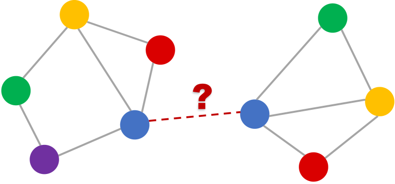
Figure 1: A toy example of entity alignment.

Entity Alignment (EA) aims to find equivalent entity pairs between KGs (as shown in Figure 1), which is the core step of bridging and integrating multi-source KGs. Therefore, EA attracts enormous attention and progresses rapidly. Most existing methods regard EA as a graph representation learning task and share the same two-stage architecture: (i) encoding the KGs into low-dimensional spaces via graph encoders (e.g., TransE Bordes et al. (2013) and GCN Kipf and Welling (2016)) and (ii) mapping the embeddings of equivalent entity pairs into a unified vector space through contrastive losses Hadsell et al. (2006).

Recently, Graph Neural Network (GNN) has achieved impressive success in many sorts of graph applications. Following Wang et al. (2018b), who first introduced Graph Convolutional Network (GCN) into EA, numerous new fancy mechanisms are proposed and stacked over vanilla GCN for better performance, such as Graph Matching Fey et al. (2020), Relational Attention Mao et al. (2020a), and Hyperbolic embedding Sun et al. (2020a). According to an EA paper list on Github, over $90\%$ of EA methods adopted GNNs as their graph encoders in recent three years.

However, there is no such thing as a free lunch. These increasingly complex GNN-based methods inherit the following inborn defects from their GNN lineage: (i) Weak scalability. Since the scales of real-world graphs are usually massive (e.g., YAGO$3$ Suchanek et al. (2007) contains $17$ million entities), the scalability of graph algorithms is crucial. However, as summarized by Zhao et al. (2020), most advanced EA methods require several hours Sun et al. (2018); Cao et al. (2019) or even days Xu et al. (2019) on the DWY$100$K dataset, which only contains $200,000$ nodes. Although an efficient loss function Mao et al. (2021a) or a graph sampler Gao et al. (2022) could effectively alleviate this problem, all existing EA methods are still overstretched when facing the real-world KGs. (ii) Poor interpretability. Interpreting neural networks is a recognized challenge, and the complex graph structure makes it more difficult. A few studies try to explain the behaviors of EA methods by showing wrong cases Yang et al. (2019a) or visualizing attention weights Wu et al. (2020). And most EA studies Sun et al. (2018); Xu et al. (2019); Mao et al. (2020b) do not attempt to give any interpretation, only focusing on improving the performances on evaluation metrics.

An ancient Chinese saying goes, "drawing new inspiration while reviewing the old." A recent study Huang et al. (2021) reinvents the classical graph algorithm — Label Propagation (LP) Zhu and Ghahramani (2002), combining it with shallow neural networks. Surprisingly, this simple method out-performs the current best-known GNNs with more than two orders of magnitude fewer parameters and more than two orders of magnitude less training time. Inspired by their excellent work, this paper proposes the Three-view Label Propagation mechanism that enables the LP algorithm, designed for homogeneous graphs, to effectively run on KGs (a kind of typical heterogeneous graph). Besides, we further propose two approximation strategies to reduce the computational complexity and enhance the scalability: Random Orthogonal Label Generation and Sparse Sinkhorn Iteration. The above three components constitute the proposed non-neural EA framework — LightEA. According to the extensive experiments on four groups of public datasets, LightEA has impressive scalability, robustness, and interpretability:

(1) Scalability: Unlike GNN-based EA methods that require multiple rounds of forward and backward propagation, LightEA only requires one round of label propagation without any trainable parameters. After abandoning neural networks, LightEA achieves extremely high parallel computing efficiency. With a PC that has one RTX$3090$ GPU, LightEA only takes $7$ seconds to obtain the alignment results on DBP$15$K and less than $35$ seconds on DWY$100$K, which is only one-tenth of the state-of-the-art EA method. LightEA could also easily handle DBP$1$M which contains more than one million entities and nearly ten million triples, while most EA methods even cannot run on it. Besides running speed, the flexible framework enables LightEA could easily incorporate iterative strategies and literal features (e.g., entity names) to improve performance.

(2) Robustness: In this paper, we design a thorough robustness examination that evaluates LightEA on four groups of public datasets containing cross-lingual, mono-lingual, sparse, dense, and large-scale subsets. With a mere tenth of time consumption, LightEA achieves comparable results to state-of-the-art methods across all datasets and even surpasses them on many. Besides, since LightEA does not have trainable parameters, the performance fluctuation of multiple runs is limited.

(3) Interpretability: Researchers generally consider linear models (e.g., Linear Regression) have decent interpretability because their outputs are the linear summation of the input features. Consistent with the LP algorithm, the computational process of LightEA is also entirely linear. After removing Random Orthogonal Label, each dimension of the label vectors will have a clear and realistic meaning. We could trace the propagation process at each step to clearly explain how the entities are aligned.

In addition to the above contributions, we further design extensive auxiliary experiments to investigate the behaviors of LightEA in various situations. The source code and datasets are now available in Github (github.com/MaoXinn/LightEA).

2 Task Definition

A KG could be defined as $\mathcal{G}=(\mathcal{E},\mathcal{R},\mathcal{T})$, where $\mathcal{E}$ is the entity set, $\mathcal{R}$ is the relation set, and $\mathcal{T}\subset\mathcal{E}\times\mathcal{R}\times\mathcal{E}$ represents the set of triples. Given the source graph $\mathcal{G}_{s}$, the target graph $\mathcal{G}_{t}$, and the set of pre-aligned entity pairs $\mathcal{P}$, EA aims to find new equivalent entity pairs based on $\mathcal{G}_{s}$, $\mathcal{G}_{t}$, and $\mathcal{P}$.

3 Related Work

3.1 Entity Alignment

Most existing methods regard EA as a graph representation learning task and share the same two-stage architecture: (i) encoding the KGs into low-dimensional spaces via graph encoders and then (ii) mapping the embeddings of equivalent entity pairs into a unified vector space by contrastive losses.

Graph encoder is the most prominent and important part of existing EA methods. Early methods usually used TransE Bordes et al. (2013) and its variants as the graph encoder. However, due to TransE only focusing on optimizing independent triples $\bm{h}+\bm{r}\approx\bm{t}$, it lacks the ability to model the global structure of KGs. With impressive capability in modeling graph data, GNNs quickly become the mainstream algorithm for almost all graph applications, including entity alignment. Since Wang et al. (2018b) first introduced GCN into EA, numerous GNN-based EA methods have been springing up. For example, GM-Align Xu et al. (2019) introduces Graph Matching Networks to capture the entity interactions across KGs. RREA Mao et al. (2020b) proposes the Relational Reflection operation to generate relation-specific entity embeddings. HyperEA Sun et al. (2020a) adopts hyperbolic embeddings to reduce the dimension of entities.

Besides the modifications on encoders, some EA methods adopt iterative strategies to generate semi-supervised data due to the lack of labeled entities. Some EA methods propose that introducing literal information (e.g., entity names) could provide a multi-aspect view for alignment models. However, it should be noted that not all KGs contain literal information, especially in practical applications. Table 1 categorizes some popular EA methods based on their encoders and whether using iterative strategies or literal information.

Method	Encoder	Literal	Iterative
MtransEChen et al. (2017)	Trans
JAPE Sun et al. (2017)	Trans
BootEA Sun et al. (2018)	Trans		✔
KDCoE Chen et al. (2018)	Trans	✔	✔
RSN Guo et al. (2019)	RNN
TransEdgeSun et al. (2020b)	Trans		✔
GCN-Align Wang et al. (2018b)	GNN
MuGNN Cao et al. (2019)	GNN
RDGCN Wu et al. (2019)	GNN	✔
GM-Align Xu et al. (2019)	GNN	✔
HyperKA Sun et al. (2020a)	GNN
MRAEA Mao et al. (2020a)	GNN		✔
RREA Mao et al. (2020b)	GNN		✔
Dual-AMN Mao et al. (2021a)	GNN		✔
EASY Ge et al. (2021b)	GNN	✔	✔
ClusterEA Gao et al. (2022)	GNN		✔

Table 1: Categorization of some popular EA methods.

3.2 Label Propagation and GCN

Label Propagation (LP) Zhu and Ghahramani (2002) is a classical graph algorithm for node classification and community detection. It assumes that two connected nodes are likely to have the same label, and thus it propagates labels along the edges. Let $\bm{A}\in\mathbb{R}^{|\mathcal{E}|\times|\mathcal{E}|}$ be the graph adjacency matrix, $\bm{D}\in\mathbb{R}^{|\mathcal{E}|\times|\mathcal{E}|}$ be the diagonal degree matrix of $\bm{A}$, $\bm{L}^{(k)}\in\mathbb{R}^{|\mathcal{E}|\times c}$ be the label matrix after $k$ rounds of label propagation, where $c$ is the number of classes. Each column of $\bm{L}^{(0)}$ is a one-hot vector, initialized by the input labels of the known nodes, while the label vectors of unknown nodes remain zeros. The propagation process of the random LP algorithm could be formulated as follow:

$$\bm{L}^{(k+1)}=\bm{D}^{-1}\bm{A}\bm{L}^{(k)}\\$$ (1)

Graph Convolutional Network (GCN) Kipf and Welling (2016) is a multi-layer neural network that propagates and transforms node features across the graph. Let $\bm{H}^{(k)}\in\mathbb{R}^{|\mathcal{E}|\times d_{in}}$ be the input features of layer $k$, and $\bm{W}^{(k)}\in\mathbb{R}^{d_{in}\times d_{out}}$ be the transformation matrix. The layer-wise propagation process of GCN could be summarized as follow:

$$\bm{H}^{(k+1)}=\sigma(\bm{D}^{-1/2}\bm{A}\bm{D}^{-1/2}\bm{H}^{(k)}\bm{W}^{(k)})\\$$ (2)

Equations (1) and (2) indicate that the common intuition behind both LP and GCN is smoothing the labels or features. Wang and Leskovec (2020) notice this kind of inner correlation and unify them into one framework. Huang et al. (2021) combine shallow neural networks with the LP algorithm, achieving comparable performances to state-of-the-art GNNs, but with a small fraction of the parameters and time consumption. These excellent works inspire us that the LP algorithm, neglected by the EA community, deserves further investigation.

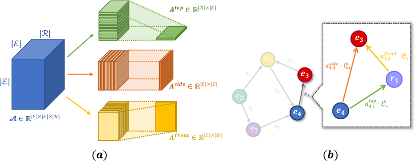
Figure 2: Illustrations of Three-view Label Propagation.

4 The Proposed Method

LightEA is a non-neural EA framework consisting of three components: (i) Random Orthogonal Label Generation, (ii) Three-view Label Propagation, and (iii) Sparse Sinkhorn Iteration. We will describe each component of LightEA in this section.

4.1 Random Orthogonal Label Generation

Different from the node classification and community detection tasks, the entities in EA do not have explicit class labels. LightEA borrows a common idea from face recognition Wang et al. (2018a); Deng et al. (2019) that regards each pair of pre-aligned entities as a independent class. Assume that $(e_{i},e_{j})\in\mathcal{P}$ is the $x$-$th$ pre-aligned entity pair, the input label matrix of entities $\bm{L}^{(0)}_{e}=\left[\bm{l}^{(0)}_{e_{1}},\bm{l}^{(0)}_{e_{2}},...,,\bm{l}^{(0)}_{e_{|\mathcal{E}|}}\right]$ is initialized as follows:

$$\bm{l}^{(0)}_{e_{i}}=\bm{l}^{(0)}_{e_{j}}=onehot(x)\;\;\;\forall(e_{i},e_{j})\in\mathcal{P}$$ (3)

where $onehot(x)\in\mathbb{R}^{|\mathcal{P}|}$ represents the one-hot vector that only the $x$-$th$ element equals one. The input label vectors of remaining unaligned entities are initialized to all-zero. Besides, since existing EA datasets do not provide pre-aligned relation pairs, the input label matrix of relations $\bm{L}^{(0)}_{r}\in\mathbb{R}^{|\mathcal{R}|\times|\mathcal{P}|}$ is also initialized to all-zero.

However, this initialization strategy will cause the input label matrices of entities and relations overly large and extremely sparse. To ensure that LightEA runs well on large-scale datasets, we have to seek a solution that could reduce the dimension of input label matrices while the loss of orthogonality is slight. Fortunately, independent random vectors on the high-dimensional hyper-sphere could satisfy our requirement.

Lemma 1

If $\bm{x}$ and $\bm{y}$ are independent random unit vectors on the $d$-dimensional hyper-sphere, $\left\langle\cdot\right\rangle$ represents the inner-product operation, then we have:

$$P\left(\langle\bm{x},\bm{y}\rangle>\epsilon\right)\leq(1-\epsilon^{2})^{(d+1)/2}$$ (4)

Lemma 4 Ball (1997) states that any two independent random vectors on the high-dimensional hyper-sphere are approximately orthogonal. For example, when $d>2048$, the probability upper bound of $\left\langle\bm{x},\bm{y}\right\rangle>0.1$ is less than $3.37\times 10^{-5}$. Therefore, LightEA independently samples random vectors on the $d$-dimensional hyper-sphere to approximate the one-hot label vectors for better space-time complexity:

$$\bm{l}^{(0)}_{e_{i}}=\bm{l}^{(0)}_{e_{j}}=random(d)\;\;\;\forall(e_{i},e_{j})\in\mathcal{P}$$ (5)

With this approximation strategy, the dimensions of $\bm{L}^{(0)}_{e}$ and $\bm{L}^{(0)}_{r}$ are reduced to $\mathbb{R}^{|\mathcal{E}|\times d}$ and $\mathbb{R}^{|\mathcal{R}|\times d}$.

One of the significant differences between LP and GCN is that one propagates labels, and the other propagates features. However, the above discussion indicates that randomly initialized features could be regarded as an approximation to one-hot labels. From this perspective, the propagation processes of GCN and LP are equivalent.

4.2 Three-view Label Propagation

Both LP algorithm and vanilla GCN were originally designed for homogeneous graphs. However, KG is a kind of typical heterogeneous graph that requires a third-order tensor $\boldsymbol{\mathcal{A}}\in\mathbb{R}^{|\mathcal{E}|\times|\mathcal{E}|\times|\mathcal{R}|}$ to fully describe its adjacency relations. Some early EA methods Wang et al. (2018b); Xu et al. (2019) crudely treat all relations as equivalent, resulting in information losses. Follow-up studies usually address this problem by adopting the relational attention mechanism Wu et al. (2019); Mao et al. (2020a) to learn attention parameters and assign different weights for different relations and triples.

Besides the above methods, an intuitive solution for generalizing LP on KGs is to use the tensor-matrix product to replace the matrix product:

$$\bm{L}^{(k+1)}_{e} =\boldsymbol{\mathcal{A}}\times_{2}\bm{L}^{(k)}_{e}\times_{3}\bm{L}^{(k)}_{r}$$ (6)

$$\bm{L}^{(k+1)}_{r} =\boldsymbol{\mathcal{A}}\times_{1}\bm{L}^{(k)}_{e}\times_{2}\bm{L}^{(k)}_{e}$$ (7)

where $\times_{i}$ represents the $i$-mode tensor-matrix product (i.e., along the $i$-$th$ axis). Unfortunately, this solution has two fatal defects: (i) The tensor-matrix product leads to a squared increase in the dimension after each round of propagation. (ii) Existing tensor computing frameworks (e.g., Tensorflow) do not provide the tensor-matrix product operator for sparse tensors.

Inspired by the three-view drawing of engineering fields, we propose a Three-view Label Propagation mechanism that compresses the adjacency tensor $\boldsymbol{\mathcal{A}}$ along three axes to retain maximum information from the original tensor while reducing computational complexity. As shown in Figure 2(a), we first separately sum the original tensor $\boldsymbol{\mathcal{A}}$ along three axes to obtain the top view $\bm{A}^{top}\in\mathbb{R}^{|\mathcal{R}|\times|\mathcal{E}|}$, the side view $\bm{A}^{side}\in\mathbb{R}^{|\mathcal{E}|\times|\mathcal{E}|}$, and the front view $\bm{A}^{front}\in\mathbb{R}^{|\mathcal{E}|\times|\mathcal{R}|}$. From the perspective of inside meaning, $\bm{A}^{side}$, $\bm{A}^{front}$, and $\bm{A}^{top}$ represent the adjacency relations from head entity to tail entity, head entity to relation, and relation to tail entity, respectively. Then, the labels of entities and relations are propagated according to the three views:

$$\bm{L}^{(k+1)}_{e} =\bm{A}^{side}\bm{L}^{(k)}_{e}+\bm{A}^{front}\bm{L}^{(k)}_{r}$$ (8)

$$\bm{L}^{(k+1)}_{r} =\bm{A}^{top}\bm{L}^{(k)}_{e}$$ (9)

Intuitively, LightEA transforms the propagation process on triples into a triangular process, where each side of the triangle represents a different view (as shown in Figure 2(b)). In this way, labels could be effectively propagated on KGs without any trainable parameters while keeping the complexity consistent with the classical LP algorithm $O(|\mathcal{T}|d)$. Finally, for each entity $e_{i}$, we concatenate the label vectors of all time-steps as the outputs:

$$\bm{l}^{out}_{e_{i}}=\left[\bm{l}^{(0)}_{e_{i}}||\bm{l}^{(1)}_{e_{i}}||...||\bm{l}^{(k-1)}_{e_{i}}||\bm{l}^{(k)}_{e_{i}}\right]$$ (10)

4.3 Sparse Sinkhorn Iteration

Early EA studies Wang et al. (2018b); Sun et al. (2017) simply calculate the Euclidean distances or cosine similarities of all entity pairs and select the closest one as the alignment result. In this way, one entity could be aligned to multiple entities simultaneously, which violates the one-to-one constraint of EA. To address this problem, some studies Xu et al. (2020); Mao et al. (2021b) transform the decoding process of EA into an assignment problem and achieve significant performance improvement:

$$\underset{\bm{P}\in\mathbb{P}_{|\mathcal{E}|}}{arg\;max}{\;\left\langle\bm{P},\bm{S}\right\rangle}_{F}$$ (11)

$\bm{S}\in\mathbb{R}^{|\mathcal{E}|\times|\mathcal{E}|}$ is the similarity matrix of entities, and $s_{i,j}=cosine(\bm{l}^{out}_{e_{i}},\bm{l}^{out}_{e_{j}})$ in LightEA. $\bm{P}$ is a permutation matrix denoting the alignment plan, where exactly one entry of $1$ in each row and column and $0$s elsewhere. $\mathbb{P}_{|\mathcal{E}|}$ represents the set of all $|\mathcal{E}|$-dimensional permutation matrices. $\langle\cdot\rangle_{F}$ represents the Frobenius inner product.

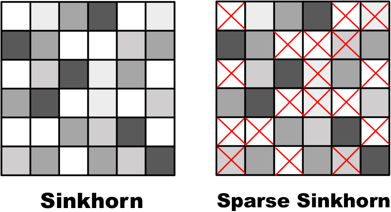
Figure 3: Sinkhorn and Sparse Sinkhorn Iteration.

Although the Hungarian algorithm Lawler (1963) could solve assignment problems accurately, its high complexity $O(|\mathcal{E}|^{3})$ makes it impossible to apply in large-scale datasets. Therefore, recent studies Ge et al. (2021b); Mao et al. (2021b) propose to use the Sinkhorn iteration Cuturi (2013) to obtain an approximate solution:

$$\begin{split}&\underset{\bm{P}\in\mathbb{P}_{|\mathcal{E}|}}{arg\;max}{\;\left\langle\bm{P},\bm{S}\right\rangle}_{F}\\ =&\lim_{\tau\rightarrow 0^{+}}{\rm Sinkhorn}(\bm{S}/\tau)\end{split}$$ (12)

The space-time complexity of the Sinkhorn iteration is $O(q|\mathcal{E}|^{2})$, where $q$ is the number of iteration rounds. Even though the Sinkhorn iteration is significantly faster than the Hungarian algorithm, it still becomes the main bottleneck of LightEA.

In LightEA, we adopt the decoding algorithm proposed by Mao et al. (2022) and utilize Sparse Sinkhorn Iteration to reduce the computational complexity. Specifically, we notice that the exponential normalization of the Sinkhorn iteration causes most smaller values in the similarity matrix $\bm{S}$ to be infinitely close to zero. Even if these smaller values are removed initially, it does not significantly affect the alignment results. Therefore, instead of calculating the similarities between all entities, LightEA only retrieves the top-$k$ nearest neighbors for each entity by Approximate Nearest Neighbor algorithms , such as Inverted Index System and Product Quantizer Jégou et al. (2011). As shown in Figure 3, the similarity matrix $\bm{S}$ will become sparse. There are only $k$ non-zero elements in each row, while the others are set to zeros. In this way, the complexity of the Sinkhorn iteration could be reduced to $O(qk|\mathcal{E}|)$.

Method	$\rm{DBP_{ZH-EN}}$			$\rm{DBP_{JA-EN}}$			$\rm{DBP_{FR-EN}}$			$\rm{SRPRS_{FR-EN}}$			$\rm{SRPRS_{DE-EN}}$
	H@1	H@10	MRR	H@1	H@10	MRR	H@1	H@10	MRR	H@1	H@10	MRR	H@1	H@10	MRR
MTransE	0.209	0.512	0.310	0.250	0.572	0.360	0.247	0.577	0.360	0.213	0.447	0.290	0.107	0.248	0.160
GCN-Align	0.434	0.762	0.550	0.427	0.762	0.540	0.411	0.772	0.530	0.243	0.522	0.340	0.385	0.600	0.460
RSNs	0.508	0.745	0.591	0.507	0.737	0.590	0.516	0.768	0.605	0.350	0.636	0.440	0.484	0.729	0.570
HyperKA	0.572	0.865	0.678	0.564	0.865	0.673	0.597	0.891	0.704	-	-	-	-	-	-
LightEA-B	0.756	0.905	0.811	0.762	0.919	0.819	0.807	0.943	0.857	0.466	0.746	0.560	0.594	0.814	0.670
BootEA	0.629	0.847	0.703	0.622	0.853	0.701	0.653	0.874	0.731	0.365	0.649	0.460	0.503	0.732	0.580
TransEdge	0.735	0.919	0.801	0.719	0.932	0.795	0.710	0.941	0.796	0.400	0.675	0.490	0.556	0.753	0.630
MRAEA	0.757	0.930	0.827	0.758	0.934	0.826	0.781	0.948	0.849	0.460	0.768	0.559	0.594	0.818	0.666
Dual-AMN	0.808	0.940	0.857	0.801	0.949	0.855	0.840	0.965	0.888	0.481	0.778	0.568	0.614	0.823	0.687
LightEA-I	0.812	0.915	0.849	0.821	0.933	0.864	0.863	0.959	0.900	0.484	0.769	0.570	0.615	0.817	0.685
GM-Align	0.679	0.785	-	0.739	0.872	-	0.894	0.952	-	0.574	0.646	0.602	0.681	0.748	0.710
RDGCN	0.697	0.842	0.750	0.763	0.897	0.810	0.873	0.950	0.901	0.672	0.767	0.710	0.779	0.886	0.820
EASY	0.898	0.979	0.930	0.943	0.990	0.960	0.980	0.998	0.990	0.965	0.989	0.970	0.974	0.992	0.980
SEU	0.900	0.965	0.924	0.956	0.991	0.969	0.988	0.999	0.992	0.982	0.995	0.986	0.983	0.996	0.987
LightEA-L	0.952	0.984	0.964	0.981	0.997	0.987	0.995	0.998	0.996	0.986	0.994	0.989	0.988	0.995	0.991

Table 2: Performances on DBP$15$K and SRPRS. Baselines’ results are from original papers or Zhao et al. (2020).

5 Experiments

All experiments are conducted on a PC with an Nvidia RTX$3090$ GPU and an EPYC 7452 CPU.

5.1 Datesets and Metrics

To comprehensively verify the scalability, robustness, and interpretability of our proposed methods, we conduct experiments on the following four groups of datasets:

(1) DBP15K Sun et al. (2017) is the most commonly used EA dataset, consisting of three small-sized cross-lingual subsets. Each subset contains $15,000$ pre-aligned entity pairs.

(2) SRPRS Guo et al. (2019) is a sparse dataset that includes two small-sized cross-lingual subsets. Each subset of SRPRS also contains $15,000$ pre-aligned entity pairs but with much fewer triples.

(3) DWY100K Sun et al. (2018) comprises two medium-sized mono-lingual subsets, each containing $100,000$ pre-aligned entity pairs and nearly one million triples.

(4) DBP1M Ge et al. (2021a) is one of the largest EA datasets so far, consisting of two cross-lingual subsets with more than one million entities and nearly ten million triples.

The detailed statistics are listed in Table 6. Consistent with the previous studies Sun et al. (2017); Wu et al. (2019); Mao et al. (2020a), we randomly split $30\%$ of the pre-aligned entity pairs for training and the remaining $70\%$ for testing. Following convention Chen et al. (2017); Wang et al. (2018b), we use $Hits@k$ and Mean Reciprocal Rank (MRR) as our evaluation metrics. The reported performances are the average of five independent runs.

5.2 Baselines

According to the categorization in Table 1, we compare LightEA against the following three groups of advanced EA methods: (1) Basic: MtransE Chen et al. (2017), GCN-Align Wang et al. (2018b), RSNs Guo et al. (2019), HyperKA Sun et al. (2020a). (2) Iterative: BootEA Sun et al. (2018), TransEdge Sun et al. (2020b), MRAEA Mao et al. (2020a), Dual-AMN Mao et al. (2021a), LargeEA Ge et al. (2021a), ClusterEA Gao et al. (2022). (3) Literal: GM-Align Xu et al. (2019), RDGCN Wu et al. (2019), SEU Mao et al. (2021b), EASY Ge et al. (2021b).

To make a fair comparison against the above methods, LightEA also has three corresponding versions: (1) LightEA-B is the basic version. (2) LightEA-I adopts the bi-directional iterative strategy proposed by Mao et al. (2020a). (3) LightEA-L uses the pre-trained word embeddings of translated entity names as the inputs matrix and also adopts the bi-directional iterative strategy. Same with SEU and EASY, LightEA-L is an unsupervised method that does not require any pre-aligned entity pairs.

5.3 Hyper-parameters

Except for DBP$1$M, we use the same setting: the dimension of hyper-sphere $d=1,024$; the number of Three-view Label Propagation rounds $k=2$. We reserve the top-$500$ nearest neighbors for each entity in Sparse Sinkhorn Iteration. Following Mao et al. (2021b), the number of Sinkhorn iteration rounds $q=10$ and the temperature $\tau=0.05$. Due to the limitation of GPU memory, the dimension of hyper-sphere $d$ is reduced to $256$ for DBP$1$M.

Method	$\rm{DWY_{DBP-WD}}$			$\rm{DWY_{DBP-YG}}$
	H@1	H@10	MRR	H@1	H@10	MRR
MTransE	0.238	0.507	0.330	0.227	0.414	0.290
GCN-Align	0.494	0.756	0.590	0.598	0.829	0.680
RSNs	0.607	0.793	0.673	0.689	0.878	0.756
MuGNN	0.604	0.894	0.701	0.739	0.937	0.810
LightEA-B	0.861	0.962	0.898	0.884	0.977	0.918
BootEA	0.748	0.898	0.801	0.761	0.894	0.808
TransEdge	0.788	0.938	0.824	0.792	0.936	0.832
MRAEA	0.794	0.930	0.856	0.819	0.951	0.875
Dual-AMN	0.869	0.969	0.908	0.907	0.981	0.935
LightEA-I	0.907	0.978	0.934	0.902	0.980	0.929

Table 3: Experimental results on DWY$100$K.

Method	$\rm{DBP1M_{FR-EN}}$			$\rm{DBP1M_{DE-EN}}$
	H@1	H@10	MRR	H@1	H@10	MRR
LargeEA-G	0.051	0.134	0.080	0.034	0.095	0.050
LargeEA-R	0.094	0.215	0.130	0.064	0.150	0.090
LargeEA-D	0.105	0.219	0.150	0.066	0.147	0.090
ClusterEA-G	0.100	0.245	0.150	0.069	0.177	0.110
ClusterEA-R	0.260	0.456	0.320	0.250	0.450	0.320
ClusterEA-D	0.281	0.474	0.350	0.288	0.488	0.350
LightEA-B	0.262	0.450	0.318	0.258	0.457	0.316
LightEA-I	0.285	0.468	0.345	0.289	0.479	0.347

Table 4: Experimental results on DBP$1$M.

5.4 Main Experiments

Table 2 lists the experimental results of LightEA on DBP$15$K and SRPRS. Table 3 and Table 6 list the results on DWY$100$K and DBP$1$M, respectively.

DBP15K. Compared to the basic EA baselines, LightEA-B has significant improvements on all metrics. The main reason is that these basic EA methods were proposed earlier, while most advanced methods adopts iterative strategies for better performance. For LightEA-I, the bi-directional iterative strategy improves the performance by more than $5\%$ on $Hits@1$ and $4\%$ on MRR. Compared to Dual-AMN, the state-of-the-art structure-based EA method, LightEA-I achieves comparable results that are slightly better on $Hits@1$ and weaker on $Hits@10$. Among literal-based EA methods, LightEA-L consistently achieves the best performances. Especially for $\rm DBP_{ZH-EN}$, LightEA-L beats SEU by more than $5\%$ on $Hits@1$.

SRPRS. The performance rankings on SRPRS are pretty similar to those on DBP$15$K. LightEA-B and LightEA-L defeat all the competitors, while LightEA-I achieves similar performances to Dual-AMN. The main difference is that the impact of iterative strategies is significantly weakened on SPRPS, in which the performance gain is less than $2\%$ on $Hits@1$ and $1\%$ on MRR. That is mainly because the structural information of SRPRS is particularly sparse, causing iterative strategies to fail to generate high-quality semi-supervised data.

DWY100K. For DWY$100$K, LightEA maintains competitive performance. On $\rm DWY_{DBP-WD}$, LightEA outperforms Dual-AMN by $4\%$ on $Hits@1$ and $3\%$ on MRR while having a comparable result on $\rm DWY_{DBP-YG}$. According to Zhao et al. (2020), the names of equivalent entities in DWY$100$K are almost identical, and using the edit distance could easily achieve the ground-truth performance. Therefore, Table 3 does not list the results of literal methods.

DBP1M. As one of the largest EA datasets so far, DBP1M poses a severe challenge to scalability, and most EA methods cannot directly run on this dataset. As shown in Table 6, the experimental results show that LightEA still achieves similar performances to the state-of-the-art method on this challenging dataset. LargeEA and ClusterEA are two acceleration frameworks for GNN-based EA methods, consisting of mini-batch graph samplers, efficient losses, etc. "-G," "-R," and "-D" represent using GCN-Align, RREA, and Dual-AMN as the backbone networks, respectively.

Method	DBP15K	SRPRS	DWY100K	DBP1M
Dual-AMN	69	57	2,237	-
LargeEA-D	26	23	227	2,119
ClusterEA-D	43	36	389	1,503
LightEA-B	2.8	2.2	15.4	97
LightEA-I	7.1	6.5	34.5	228
LightEA-L	14.8	11.2	-	-

Table 5: Time costs on all datasets (seconds).

Time cost. Table 5 reports the time costs of three variants of LightEA. Due to the space limitation, we only list out the time costs of Dual-AMN with two acceleration frameworks as the baselines. For the results of other EA methods, please refer to Table 7 in Appendix C. LargeEA and ClusterEA effectively accelerate Dual-AMN, achieving ten times speedups on DBP$1$M. However, GNN-based methods are still stuck with multiple rounds of forward and backward propagation, while LightEA only requires one round of label propagation and no need for training. With similar performances, the time consumption of LightEA-B is less than one-seventh of Dual-AMN variants. Besides, introducing iterative strategies and literal features significantly increases time consumption while also improving performance.

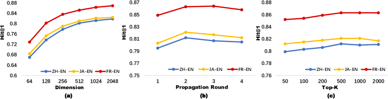
Figure 4: Hyper-parameter experiments of LightEA-I on DBP$15$K.

5.5 Hyper-parameters

We design extensive hyper-parameter experiments to investigate the behaviors of LightEA in various situations. Due to the space limitation, Figure 4 only shows the results of LightEA-I on DBP$15$K. Appendix D shows the results on other datasets.

Dimension. To alleviate the problem that one-hot label vectors being over-sparse, LightEA proposes to replace them with independent random vectors on high-dimensional hyper-spheres. Figure 4(a) shows the $Hits@1$ curves with different dimensions $d$. Clearly, there are significant diminishing marginal effects on increasing dimensions. When the dimension $d>1,024$, the performance gain becomes limited. Actually, the reason behind diminishing marginal effects has been told by Lemma 4 — the probability of two random drawn vectors "conflicting" with each other (i.e., $\langle\bm{x},\bm{y}\rangle>\epsilon$) decreases exponentially as the dimension $d$ increases.

Propagation Round. Figure 4(b) shows the performances with different numbers of propagation rounds. Similar to the network depth of GNNs, more propagation rounds also lead to the over-smoothing problem. When the number of rounds $q=2$, LightEA-I achieves the best performance and then begins to decline. This phenomenon indicates a high correlation between label propagation and GNNs from the side.

Top-K. In Sparse Sinkhorn Iteration, LightEA only retrieves the top-$k$ nearest neighbors for each entity instead of calculating the distances between all pairs. As expected, Figure 4(c) shows that removing smaller values from the similarity matrix hardly affects the alignment performances. The trick of Sparse Sinkhorn Iteration could reduce the space-time complexity with limited losses.

Besides hyper-parameters, we further design more auxiliary experiments, such as ablation experiments. Due to the space limitation, these experiments are listed in Appendix E, F, and G.

5.6 How to Interpret the Results

Existing GNN-based EA methods inherit poor interpretability from neural networks. It is hard to explain the inside meaning of each dimension of entity features and why two entities are aligned. Therefore, the output features are only used to calculate the similarities. Different from GNN-based methods, we could clearly interpret the alignment results of LightEA by the following steps:

(1) Remove Random Orthogonal Label. After removing this component, the meaning of each dimension of label vectors becomes clear and realistic. The $x$-$th$ dimension of $\bm{l}_{e_{i}}^{(k)}$ represents the relevance score between $e_{i}$ and the $x$-$th$ pre-aligned entity pair after $k$ rounds of propagation. If two entities are equivalent, their distributions of relevance scores should also be similar.

(2) Trace the propagation: Since we have known the meaning of each dimension, we could trace the propagation process at each time-step to investigate why two entities are aligned.

However, removing the Random Orthogonal Label Generation will make the label matrices extremely large and sparse, and the Three-view Label Propagation can only run on the small-sized sub-graphs. Therefore, this strategy only fits for interpreting a limited number of entities.

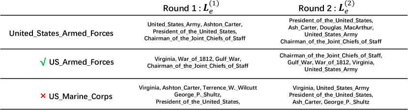
Figure 5: An example of tracing the propagation process and interpreting the alignment results.

5.7 An Example of Tracing the Wrong Case

Figure 5 shows an example of tracing the propagation process and interpreting the alignment results. In this case, United_States_Armed_Forces is incorrectly aligned with US_Marine_Corps, and the correct answer is US_Armed_Forces.

As described in last section, we first remove the Random Orthogonal Label, run the Three-view Label Propagation, and obtain the sparse label matrices $\bm{L}^{(1)}_{e}$ and $\bm{L}^{(2)}_{e}$. Then, we separately sort the label vectors $\bm{l}^{(1)}_{e_{i}}$ and $\bm{l}^{(2)}_{e_{i}}$ of each entity to get the dimension indexes of top-$5$ non-zero elements. Finally, we look up the corresponding names of dimension indexes in the entity name list and show them in Figure 5. Apparently, the noise of graph structure causes this wrong case. Compared to the correct entity, the incorrect entity has a more similar neighborhood structure to United_States_Armed_Forces. There are five common elements between the wrong alignment pair, while only three between the right alignment pair.

6 Conclusion

In this paper, we reinvent the Label Propagation algorithm to effectively run on KGs and propose a non-neural EA framework — LightEA. According to the experiments on public datasets, LightEA has impressive scalability, robustness, and interpretability. With a mere tenth of time consumption, LightEA achieves comparable results to state-of-the-art methods across all datasets.

Limitations

Although we have demonstrated that LightEA has impressive scalability, robustness, and interpretability on multiple public datasets with different scales, there are still three limitations that should be addressed in the future:

(1) In LightEA, good interpretability and high efficiency cannot coexist. If not removing the Random Orthogonal Label, LightEA’s interpretability will be significantly weakened. How to balance the interpretability and efficiency is our future work.

(2) Theoretically, LightEA has high parallel efficiency that could obtain linear speedup with multiple GPUs. However, we do not have enough devices to verify this advantage, and all the experiments in this paper run with a single RTX3090. We will purchase more devices to complete these missing experiments in the future.

(3) Currently, we implement LightEA via Tensorflow. Since LightEA is a non-neural algorithm without any trainable parameters, a complex deep learning framework would be redundant and inefficient. In the future, we will refactor LightEA with CUDA and C++ to further improve efficiency.

Ethics Statement

To the best of our knowledge, this work does not involve any discrimination, social bias, or private data. All the datasets are open-source and constructed from open-source KGs such as Wikidata, YAGO, and DBpedia. Therefore, we believe that our study complies with the ACL Ethics Policy. In addition, introducing literal features may cause concerns about the misuse of user-generated content. LightEA can avoid this concern by using pure structural information for entity alignment.

Ethics Statement

We appreciate the support from National Natural Science Foundation of China with the Research Project on Human Behavior in Human-Machine Collaboration (Project Number: 72192824) and the support from Pudong New Area Science & Technology Development Fund (Project Number: PKX2021-R05).

Appendix A Sinkhorn Iteration

$$\begin{split}{\rm Sink}^{(0)}(\bm{S})&=\exp(\bm{S}),\\ {\rm Sink}^{(q)}(\bm{S})&={\mathcal{N}}_{c}({\mathcal{N}}_{r}({\rm Sink}^{(q-1)}(\bm{S}))),\\ {\rm Sinkhorn}(\bm{S})&=\lim_{q\rightarrow\infty}{\rm Sink}^{(q)}(\bm{S}).\end{split}$$ (13)

here ${\mathcal{N}}_{r}(\bm{S})$$=$$\bm{S}\varoslash(\bm{S}\bm{1}_{N}\bm{1}_{N}^{T})$ and ${\mathcal{N}}_{c}$$=$$\bm{S}\varoslash(\bm{1}_{N}\bm{1}_{N}^{T}\bm{S})$ are the row and column-wise normalization operators of a matrix, $\varoslash$ represents the element-wise division, and $\bm{1}_{N}$ is a column vector of ones.

Appendix B Datasets

Datasets		$|\mathcal{E}|$	$|\mathcal{R}|$	$|\mathcal{T}|$
$\rm{DBP_{ZH-EN}}$	ZH	19,388	1,701	70,414
	EN	19,572	1,323	95,142
$\rm{DBP_{JA-EN}}$	JA	19,814	1,299	77,214
	EN	19,780	1,153	93,484
$\rm{DBP_{FR-EN}}$	FR	19,661	903	105,998
	EN	19,993	1,208	115,722
$\rm{DWY_{DBP-YG}}$	DBP	100,000	302	428,952
	YG	100,000	31	502,563
$\rm{DWY_{DBP-WD}}$	DBP	100,000	330	463,294
	Wiki	100,000	220	448,774
$\rm{SRPRS_{FR-EN}}$	FR	15,000	177	33,532
	EN	15,000	221	36,508
$\rm{SRPRS_{DE-EN}}$	DE	15,000	120	37,377
	EN	15,000	222	38,363
$\rm{DBP1M_{FR-EN}}$	FR	1,365,118	380	2,997,457
	EN	1,877,793	603	7,031,172
$\rm{DBP1M_{DE-EN}}$	DE	1,112,970	241	1,994,876
	EN	1,625,999	597	6,213,639

Table 6: Statistical data of all datasets.

Appendix C Time Costs

Method	DBP15K	SRPRS	DWY100K
MTransE	6,467	3,355	70,085
GCN-Align	103	87	3,212
RSNs	7,539	2,602	28,516
MuGNN	3,156	2,215	47,735
KECG	3,724	1,800	125,386
BootEA	4,661	2,659	64,471
NAEA	19,115	11,746	-
TransEdge	3,629	1,210	20,839
MRAEA	3,894	1,248	23,275
GM-Align	26,328	13,032	459,715
RDGCN	6,711	886	-
HMAN	5,455	4,424	31,895
HGCN	11,275	2,504	60,005

Table 7: Time costs of existing EA methods (seconds). Because we do not have enough time and devices to run all these methods by ourselves, these time costs are from the summary Zhao et al. (2020) for reference only.

Appendix D Hyper-parameter

Figure 6 shows the remaining hyper-parameter experiments on DWY$100$K and SRPRS. The performance curves on DWY$100$K are quite similar to those on DBP$15$K because the graph densities of these two datasets are close. On SRPRS, we notice that these three hyper-parameters do not significantly impact performance because SRPRS is a highly sparse and small-sized dataset. Due to the limitation of GPU memory, we do not experiment on DBP$1$M, and we will try our best to supplement these experiments in the future.

Appendix E Pre-aligned Ratio

In practice, manually annotating pre-aligned entity pairs is labor-consuming, especially for large-scale KGs. Therefore, we hope the proposed EA methods could maintain decent performances with limited pre-aligned entity pairs. To investigate the behaviors of LightEA with different pre-aligned ratios, we set the ratios from $10\%$ to $50\%$. Figure 7 shows the $Hits@1$ performances of LightEA-B and LightEA-I on DBP$15K$, DWY$100$K, and SRPRS. Even if only 10% of the entity pairs are reserved as the training data, LightEA still achieves decent performances. Besides, the iterative strategy effectively improves performance and alleviates the need for pre-aligned pairs on all datasets.

Appendix F Ablation Study

We design the following ablation experiment to demonstrate the effectiveness of each component of LightEA: (i) Remove the front view $\bm{A}^{front}$ and the top view $\bm{A}^{top}$. Thus, the Three-view Label Propagation will be degraded into the classical LP. (ii) Remove the Sparse Sinkhorn Iteration and select the closest entity as the alignment result. Due to the limitation of GPU memory, the Random Orthogonal Label cannot be removed. Table 8 shows the ablation results. Obviously, both two components are necessary, and removing either one will cause significant performance degradation.

Method	$\rm{DBP_{ZH-EN}}$		$\rm{DBP_{JA-EN}}$		$\rm{DBP_{FR-EN}}$
	Hits@1	MRR	Hits@1	MRR	Hits@1	MRR
LightEA-I	0.812	0.849	0.821	0.864	0.863	0.900
-Three-view	0.537	0.588	0.606	0.580	0.574	0.623
-Sinkhorn	0.664	0.739	0.638	0.722	0.666	0.748

Table 8: Ablation study of LightEA.

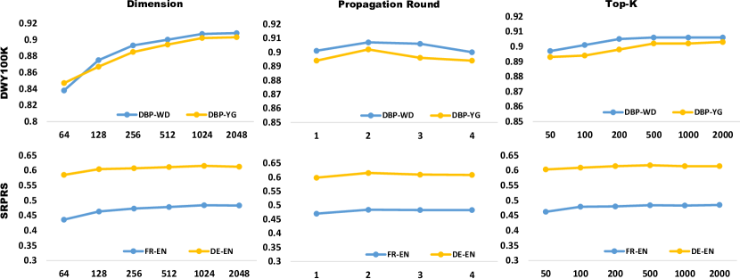
Figure 6: Hyper-parameter experiments of LightEA-I on DWY$100$K and SRPRS.

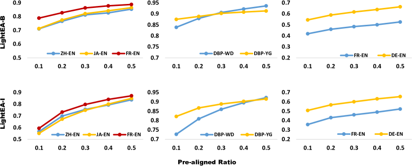
Figure 7: Hits@1 performances with different pre-aligned ratios on DBP$15$K, DWY$100$K, and SRPRS.

Table 9: Statistical data of the OpenEA benchmark.

Appendix G OpenEA Benchmark (v2.0)

Dataset	LightEA-B			LightEA-I
	H@1	H@10	MRR	H@1	H@10	MRR
EN-FR-15K-V1	0.607	0.867	0.697	0.670	0.895	0.748
EN-FR-15K-V2	0.826	0.960	0.875	0.913	0.986	0.941
EN-FR-100K-V1	0.462	0.714	0.544	0.507	0.736	0.581
EN-FR-100K-V2	0.765	0.917	0.819	0.830	0.943	0.871
EN-DE-15K-V1	0.760	0.938	0.821	0.781	0.947	0.840
EN-DE-15K-V2	0.919	0.974	0.939	0.951	0.987	0.965
EN-DE-100K-V1	0.581	0.793	0.650	0.604	0.805	0.670
EN-DE-100K-V2	0.822	0.916	0.855	0.863	0.938	0.890
D-W-15K-V1	0.663	0.867	0.737	0.732	0.902	0.796
D-W-15K-V2	0.924	0.990	0.949	0.951	0.995	0.968
D-W-100K-V1	0.588	0.796	0.659	0.642	0.833	0.707
D-W-100K-V2	0.874	0.962	0.906	0.926	0.983	0.947
D-Y-15K-V1	0.770	0.891	0.817	0.826	0.927	0.864
D-Y-15K-V2	0.976	0.995	0.983	0.976	0.996	0.983
D-Y-100K-V1	0.758	0.916	0.811	0.781	0.931	0.832
D-Y-100K-V2	0.961	0.990	0.972	0.977	0.996	0.984

Table 10: Experimental results on OpenEA (v2.0).

To make a fair and realistic comparison, OpenEA Sun et al. (2020c) constructs a well-designed evaluation benchmark. As shown in Table 9, this benchmark contains two cross-lingual settings extracted from multi-lingual DBpedia (English-to-French and English-to-German) and two mono-lingual settings among popular KGs (DBpedia-to-Wikidata and DBpedia-to-YAGO). Each setting has two scales with $15$K and $100$K entity pairs, respectively. Besides, each subset is further divided into two versions with different densities. V$1$ represents the sparse version, and V$2$ represents the dense version. The average degree of the V$1$ datasets is about half of the V$2$ datasets.

Recently, Sun et al. (2020c) released a new version (v2.0) of the OpenEA benchmark, where the URIs of DBpedia and YAGO entities are encoded to resolve the name bias issue. They strongly recommend using the v2.0 benchmark for evaluating EA methods, such that the results can better reflect the robustness of these methods in real-world situations. Since this benchmark was released recently, the performances of most baselines on this benchmark are still unclear, and we do not have enough time and devices to reproduce all the baselines on this benchmark. Therefore, Table 10 only reports the performances of our proposed method to offer a reference for follow-up research. Here, we follow the data splits in OpenEA, where 20% of alignment entity pairs are for training, 10% for validation, and 70% for testing. The setting of hyper-parameters follows Section 5.3.

References

- Ball (1997) Keith Ball. 1997. An elementary introduction to modern convex geometry.
- Bordes et al. (2013) Antoine Bordes, Nicolas Usunier, Alberto García-Durán, Jason Weston, and Oksana Yakhnenko. 2013. Translating embeddings for modeling multi-relational data. In Advances in Neural Information Processing Systems 26: 27th Annual Conference on Neural Information Processing Systems 2013. Proceedings of a meeting held December 5-8, 2013, Lake Tahoe, Nevada, United States, pages 2787–2795.
- Cao et al. (2019) Yixin Cao, Zhiyuan Liu, Chengjiang Li, Zhiyuan Liu, Juanzi Li, and Tat-Seng Chua. 2019. Multi-channel graph neural network for entity alignment. In Proceedings of the 57th Conference of the Association for Computational Linguistics, ACL 2019, Florence, Italy, July 28- August 2, 2019, Volume 1: Long Papers, pages 1452–1461.
- Chen et al. (2018) Muhao Chen, Yingtao Tian, Kai-Wei Chang, Steven Skiena, and Carlo Zaniolo. 2018. Co-training embeddings of knowledge graphs and entity descriptions for cross-lingual entity alignment. In Proceedings of the Twenty-Seventh International Joint Conference on Artificial Intelligence, IJCAI 2018, July 13-19, 2018, Stockholm, Sweden, pages 3998–4004. ijcai.org.
- Chen et al. (2017) Muhao Chen, Yingtao Tian, Mohan Yang, and Carlo Zaniolo. 2017. Multilingual knowledge graph embeddings for cross-lingual knowledge alignment. In Proceedings of the Twenty-Sixth International Joint Conference on Artificial Intelligence, IJCAI 2017, Melbourne, Australia, August 19-25, 2017, pages 1511–1517.
- Cuturi (2013) Marco Cuturi. 2013. Sinkhorn distances: Lightspeed computation of optimal transport. In Advances in Neural Information Processing Systems 26: 27th Annual Conference on Neural Information Processing Systems 2013. Proceedings of a meeting held December 5-8, 2013, Lake Tahoe, Nevada, United States, pages 2292–2300.
- Deng et al. (2019) Jiankang Deng, Jia Guo, Niannan Xue, and Stefanos Zafeiriou. 2019. Arcface: Additive angular margin loss for deep face recognition. In IEEE Conference on Computer Vision and Pattern Recognition, CVPR 2019, Long Beach, CA, USA, June 16-20, 2019, pages 4690–4699. Computer Vision Foundation / IEEE.
- Fey et al. (2020) Matthias Fey, Jan Eric Lenssen, Christopher Morris, Jonathan Masci, and Nils M. Kriege. 2020. Deep graph matching consensus. In 8th International Conference on Learning Representations, ICLR 2020, Addis Ababa, Ethiopia, April 26-30, 2020.
- Gao et al. (2022) Yunjun Gao, Xiaoze Liu, Junyang Wu, Tianyi Li, Pengfei Wang, and Lu Chen. 2022. Clusterea: Scalable entity alignment with stochastic training and normalized mini-batch similarities. CoRR, abs/2205.10312.
- Ge et al. (2021a) Congcong Ge, Xiaoze Liu, Lu Chen, Baihua Zheng, and Yunjun Gao. 2021a. Largeea: Aligning entities for large-scale knowledge graphs. Proc. VLDB Endow., 15(2):237–245.
- Ge et al. (2021b) Congcong Ge, Xiaoze Liu, Lu Chen, Baihua Zheng, and Yunjun Gao. 2021b. Make it easy: An effective end-to-end entity alignment framework. In SIGIR ’21: The 44th International ACM SIGIR Conference on Research and Development in Information Retrieval, Virtual Event, Canada, July 11-15, 2021, pages 777–786. ACM.
- Guo et al. (2019) Lingbing Guo, Zequn Sun, and Wei Hu. 2019. Learning to exploit long-term relational dependencies in knowledge graphs. In Proceedings of the 36th International Conference on Machine Learning, ICML 2019, 9-15 June 2019, Long Beach, California, USA, pages 2505–2514.
- Hadsell et al. (2006) Raia Hadsell, Sumit Chopra, and Yann LeCun. 2006. Dimensionality reduction by learning an invariant mapping. In 2006 IEEE Computer Society Conference on Computer Vision and Pattern Recognition (CVPR 2006), 17-22 June 2006, New York, NY, USA, pages 1735–1742.
- Huang et al. (2021) Qian Huang, Horace He, Abhay Singh, Ser-Nam Lim, and Austin R. Benson. 2021. Combining label propagation and simple models out-performs graph neural networks. In 9th International Conference on Learning Representations, ICLR 2021, Virtual Event, Austria, May 3-7, 2021. OpenReview.net.
- Jégou et al. (2011) Hervé Jégou, Matthijs Douze, and Cordelia Schmid. 2011. Product quantization for nearest neighbor search. IEEE Trans. Pattern Anal. Mach. Intell., 33(1):117–128.
- Johnson et al. (2019) Jeff Johnson, Matthijs Douze, and Hervé Jégou. 2019. Billion-scale similarity search with GPUs. IEEE Transactions on Big Data, 7(3):535–547.
- Kipf and Welling (2016) Thomas N. Kipf and Max Welling. 2016. Semi-supervised classification with graph convolutional networks. CoRR, abs/1609.02907.
- Lawler (1963) Eugene L Lawler. 1963. The quadratic assignment problem. Management science, 9(4):586–599.
- Mao et al. (2022) Xin Mao, Meirong Ma, Hao Yuan, Jianchao Zhu, Zongyu Wang, Rui Xie, Wei Wu, and Man Lan. 2022. An effective and efficient entity alignment decoding algorithm via third-order tensor isomorphism. In ACL.
- Mao et al. (2021a) Xin Mao, Wenting Wang, Yuanbin Wu, and Man Lan. 2021a. Boosting the speed of entity alignment 10 ×: Dual attention matching network with normalized hard sample mining. In WWW ’21: The Web Conference 2021, Virtual Event / Ljubljana, Slovenia, April 19-23, 2021, pages 821–832. ACM / IW3C2.
- Mao et al. (2021b) Xin Mao, Wenting Wang, Yuanbin Wu, and Man Lan. 2021b. From alignment to assignment: Frustratingly simple unsupervised entity alignment. In Proceedings of the 2021 Conference on Empirical Methods in Natural Language Processing, EMNLP 2021, Virtual Event / Punta Cana, Dominican Republic, 7-11 November, 2021, pages 2843–2853. Association for Computational Linguistics.
- Mao et al. (2020a) Xin Mao, Wenting Wang, Huimin Xu, Man Lan, and Yuanbin Wu. 2020a. MRAEA: an efficient and robust entity alignment approach for cross-lingual knowledge graph. In WSDM ’20: The Thirteenth ACM International Conference on Web Search and Data Mining, Houston, TX, USA, February 3-7, 2020, pages 420–428.
- Mao et al. (2020b) Xin Mao, Wenting Wang, Huimin Xu, Yuanbin Wu, and Man Lan. 2020b. Relational reflection entity alignment. In CIKM ’20: The 29th ACM International Conference on Information and Knowledge Management, Virtual Event, Ireland, October 19-23, 2020, pages 1095–1104. ACM.
- Suchanek et al. (2007) Fabian M. Suchanek, Gjergji Kasneci, and Gerhard Weikum. 2007. Yago: a core of semantic knowledge. In Proceedings of the 16th International Conference on World Wide Web, WWW 2007, Banff, Alberta, Canada, May 8-12, 2007, pages 697–706. ACM.
- Sun et al. (2020a) Zequn Sun, Muhao Chen, Wei Hu, Chengming Wang, Jian Dai, and Wei Zhang. 2020a. Knowledge association with hyperbolic knowledge graph embeddings. In Proceedings of the 2020 Conference on Empirical Methods in Natural Language Processing, EMNLP 2020, Online, November 16-20, 2020, pages 5704–5716. Association for Computational Linguistics.
- Sun et al. (2017) Zequn Sun, Wei Hu, and Chengkai Li. 2017. Cross-lingual entity alignment via joint attribute-preserving embedding. In The Semantic Web - ISWC 2017 - 16th International Semantic Web Conference, Vienna, Austria, October 21-25, 2017, Proceedings, Part I, volume 10587 of Lecture Notes in Computer Science, pages 628–644. Springer.
- Sun et al. (2018) Zequn Sun, Wei Hu, Qingheng Zhang, and Yuzhong Qu. 2018. Bootstrapping entity alignment with knowledge graph embedding. In Proceedings of the Twenty-Seventh International Joint Conference on Artificial Intelligence, IJCAI 2018, July 13-19, 2018, Stockholm, Sweden, pages 4396–4402.
- Sun et al. (2020b) Zequn Sun, JiaCheng Huang, Wei Hu, Muchao Chen, Lingbing Guo, and Yuzhong Qu. 2020b. Transedge: Translating relation-contextualized embeddings for knowledge graphs. CoRR, abs/2004.13579.
- Sun et al. (2020c) Zequn Sun, Qingheng Zhang, Wei Hu, Chengming Wang, Muhao Chen, Farahnaz Akrami, and Chengkai Li. 2020c. A benchmarking study of embedding-based entity alignment for knowledge graphs. Proc. VLDB Endow., 13(11):2326–2340.
- Wang et al. (2018a) Feng Wang, Jian Cheng, Weiyang Liu, and Haijun Liu. 2018a. Additive margin softmax for face verification. IEEE Signal Process. Lett., 25(7):926–930.
- Wang and Leskovec (2020) Hongwei Wang and Jure Leskovec. 2020. Unifying graph convolutional neural networks and label propagation. CoRR, abs/2002.06755.
- Wang et al. (2018b) Zhichun Wang, Qingsong Lv, Xiaohan Lan, and Yu Zhang. 2018b. Cross-lingual knowledge graph alignment via graph convolutional networks. In Proceedings of the 2018 Conference on Empirical Methods in Natural Language Processing, Brussels, Belgium, October 31 - November 4, 2018, pages 349–357.
- Wu et al. (2019) Yuting Wu, Xiao Liu, Yansong Feng, Zheng Wang, Rui Yan, and Dongyan Zhao. 2019. Relation-aware entity alignment for heterogeneous knowledge graphs. In Proceedings of the Twenty-Eighth International Joint Conference on Artificial Intelligence, IJCAI 2019, Macao, China, August 10-16, 2019, pages 5278–5284.
- Wu et al. (2020) Yuting Wu, Xiao Liu, Yansong Feng, Zheng Wang, and Dongyan Zhao. 2020. Neighborhood matching network for entity alignment. In Proceedings of the 58th Annual Meeting of the Association for Computational Linguistics, ACL 2020, Online, July 5-10, 2020, pages 6477–6487. Association for Computational Linguistics.
- Xu et al. (2020) Kun Xu, Linfeng Song, Yansong Feng, Yan Song, and Dong Yu. 2020. Coordinated reasoning for cross-lingual knowledge graph alignment. In The Thirty-Fourth AAAI Conference on Artificial Intelligence, AAAI 2020, The Thirty-Second Innovative Applications of Artificial Intelligence Conference, IAAI 2020, The Tenth AAAI Symposium on Educational Advances in Artificial Intelligence, EAAI 2020, New York, NY, USA, February 7-12, 2020, pages 9354–9361. AAAI Press.
- Xu et al. (2019) Kun Xu, Liwei Wang, Mo Yu, Yansong Feng, Yan Song, Zhiguo Wang, and Dong Yu. 2019. Cross-lingual knowledge graph alignment via graph matching neural network. In Proceedings of the 57th Conference of the Association for Computational Linguistics, ACL 2019, Florence, Italy, July 28- August 2, 2019, Volume 1: Long Papers, pages 3156–3161.
- Yang et al. (2019a) Hsiu-Wei Yang, Yanyan Zou, Peng Shi, Wei Lu, Jimmy Lin, and Xu Sun. 2019a. Aligning cross-lingual entities with multi-aspect information. In Proceedings of the 2019 Conference on Empirical Methods in Natural Language Processing and the 9th International Joint Conference on Natural Language Processing, EMNLP-IJCNLP 2019, Hong Kong, China, November 3-7, 2019, pages 4430–4440.
- Yang et al. (2020) Shiquan Yang, Rui Zhang, and Sarah M. Erfani. 2020. Graphdialog: Integrating graph knowledge into end-to-end task-oriented dialogue systems. In Proceedings of the 2020 Conference on Empirical Methods in Natural Language Processing, EMNLP 2020, Online, November 16-20, 2020, pages 1878–1888. Association for Computational Linguistics.
- Yang et al. (2019b) Yueji Yang, Divyakant Agrawal, H. V. Jagadish, Anthony K. H. Tung, and Shuang Wu. 2019b. An efficient parallel keyword search engine on knowledge graphs. In 35th IEEE International Conference on Data Engineering, ICDE 2019, Macao, China, April 8-11, 2019, pages 338–349. IEEE.
- Zhao et al. (2020) X. Zhao, W. Zeng, J. Tang, W. Wang, and F. Suchanek. 2020. An experimental study of state-of-the-art entity alignment approaches. IEEE Transactions on Knowledge and Data Engineering, pages 1–1.
- Zhu and Ghahramani (2002) Xiaojin Zhu and Zoubin Ghahramani. 2002. Learning from labeled and unlabeled data with label propagation.