p³VAE: a physics-integrated generative model
Application to the pixel-wise classification of airborne hyperspectral images

Abstract

The combination of machine learning models with physical models is a recent research path to learn robust data representations. In this paper, we introduce p³VAE, a generative model that integrates a physical model which deterministically models some of the true underlying factors of variation in the data. To fully leverage our hybrid design, we enhance an existing semi-supervised optimization technique and introduce a new inference scheme that comes along meaningful uncertainty estimates. We apply p³VAE to the pixel-wise classification of airborne hyperspectral images. Our experiments on simulated and real data demonstrate the benefits of our hybrid model against conventional machine learning models in terms of extrapolation capabilities and interpretability. In particular, we show that p³VAE naturally has high disentanglement capabilities. Our code and data have been made publicly available at https://github.com/Romain3Ch216/p3VAE.

1 Introduction

Hybrid modeling, that is the combination of data-driven and theory-driven modeling, has recently raised a lot of attention. The integration of physical models in machine learning has indeed demonstrated promising properties such as improved interpolation and extrapolation capabilities and increased interpretability [1, 2]. Conventional machine learning models learn correlations, from a training data set, in order to map observations to targets or latent representations, with the hope to generalize to new data. While many different models could perfectly fit the training data, the assumptions made during the learning process (from the model architecture to the learning algorithm itself), sometimes called inductive biases [3, 4], are crucial to obtain high generalization performances. In contrast, hybrid models are partially grounded on deductive biases, i.e. assumptions derived, in our context, from physics models that generalize, by nature, to out-of-distribution data. Therefore, in various fields for which the data distribution is governed by physical laws, such as fluid dynamics, thermodynamics or solid mechanics, hybrid modeling has recently become a hot topic [5, 6, 7].

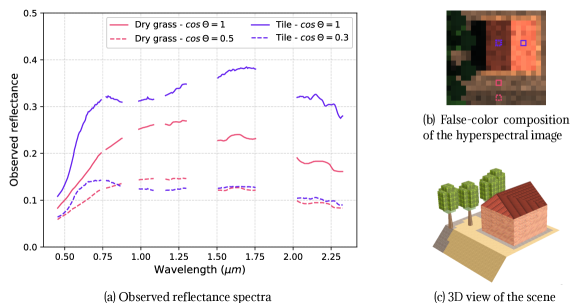
Figure 1: Illustration of intra-class variabilities and inter-class similarities due to different pixel-wise irradiance conditions. $\Theta$ is the solar incidence angle. The lower is $\Theta$, the higher is the direct irradiance.

In the present paper, we introduce p³VAE, a physics-integrated generative model that combines an assumed perfect physical model with a machine learning model. p³VAE aims to decouple the variation factors that are intrinsic to the data from physical factors related to acquisition conditions. On the hypothesis that acquisition conditions induce complex and non-linear data variations, we argue that a conventional generative model would hardly decorrelate intrinsic factors from physical factors. Therefore, we introduce deductive physics-based biases in the decoding part of a semi-supervised variational autoencoder. Variational AutoEncoders (VAEs) [8] are powerful latent variable probabilistic models that have an autoencoder framework. The key to their success lies in their stochastic variational inference and learning algorithm that allows to leverage very large unlabeled data sets and to model complex posterior data distributions given latent variables [8]. Besides, recent advances offer more and more control on the latent space distributions [9, 10, 11, 12]. VAEs were used, for instance, in text modeling to capture topic information as a Dirichlet latent variable [13] or in image modeling where latent variables were both discrete and continuous [14].

Integrating physics in an autoencoder was first proposed by [15]. They used a fully physical model inplace the decoder to inverse a 2D exponential light galaxy profile model. [2] generalized the work of [15] by developing a mathematical formalism introduced as physics-integrated VAEs ($\phi$-VAE). $\phi$-VAEs complement an imperfect physical model with a machine learning model in the decoder of a VAE. To have a consistent use of physics despite the high representation power of machine learning models, they employ a regularization strategy that is central to their contribution. In contrast, p³VAE integrates a perfect physics model that partially captures the factors of variations.

As an example of application, we apply p³VAE to the land cover classification of airborne hyperspectral images, which have a very high spatial and spectral resolutions on a wide spectral domain. We consider hyperspectral images provided in ground-level reflectance, which is a physical property intrinsic to matter and therefore highly informative of the land cover (e.g. tile, bare soil, grass…). However, without knowledge of the local (i.e. pixel-wise) irradiance conditions (that depend on topography), one material can have totally different reflectance estimates. Fig. 1 shows examples of reflectance spectra observations for two materials with different local slopes (i.e. different irradiance). Those examples illustrate how wide the spectral irradiance-based variability can be and how reflectance spectra from different classes can look alike in specific irradiance conditions. Additionally, the reflectance of one material can change based on various physical parameters such as its surface roughness, humidity or chemical composition (e.g. chlorophyll content of vegetation). We will refer to this kind of variability as intrinsic intra-class variability. Capturing the irradiance-based and the intrinsic intra-class variabilities in a supervised setting is very challenging because labeled remote sensing data is often scarce. Labeling pixels with land cover classes of low abstraction indeed require expensive field campaigns and time-consuming photo-interpretation by experts (that can distinguish materials based on their spectrum, as far as the spatial information provide little discriminating information). Therefore, only few thousands pixels are usually labeled out of many millions, which has dramatically hindered the use of machine learning algorithms.

The main contributions of the paper are as follows:

• We introduce p³VAE, a variational autoencoder that combines conventional neural network layers with physics-based layers for generative modeling,

• We enhance the semi-supervised training procedure introduced in [16] to balance between physics and trainable parameters of p³VAE,

• We introduce an inference procedure to fully leverage the physics part of p³VAE,

• We apply our model to the pixel-wise classification of airborne hyperspectral images and experimentally compare its performances against conventional machine learning models in terms of classification accuracy (interpolation and extrapolation capabilities), disentanglement, and latent variables interpretability.

Our paper is organized as follows. Section 2 discusses the related work. Section 3 presents our model in details. Section 4 describes the simulated and real data sets. We present and discuss the experiments in section 5 and 6, respectively. Finally, we conclude in section 7.

2 Related work

Our method makes use, at the same time, of physical priors and of a semi-supervised learning technique, which is intrinsically linked to the architecture of p³VAE. Therefore, we review related work on hybrid modeling and semi-supervised learning.

2.1 Hybrid modeling

Hybrid modeling can be divided into physics-based losses [17, 18, 6, 1] and physics-based models, in which our method fits. Physics-based models embed physical layers in their design. [19] and [20] introduced VAEs which latent variables were grounded to physical quantities (such as position and velocity) and governed by Ordinary Differential Equations (ODEs). More related to our work, [15] solves an inverse problem by using a conventional autoencoder in which they substitute the decoder by a fully physical model. They demonstrated that the architecture of the decoder induces a natural disentanglement of the latent space. This model is a particular case of the formalism of physics-integrated VAEs introduced by [2], that is the most closely related work to our methodology. Physics-integrated VAEs ($\phi$-VAE) are variational autoencoders which decoders combine statistical and physical models. The key idea of [2] is that the combination of an imperfect physical model with a machine learning model gives more precise results than an imperfect physical model alone and better generalization performances than a machine learning model alone. More precisely, they showed that the deductive biases introduced by the physical model regularize the machine learning model, yielding more robust local optima. Because neural networks, with powerful representation power, could bypass the physical part to model the data, they introduced a specific training procedure. Their optimization scheme aims to balance the power of the neural network so that it models the residual error of the physics model. $\phi$-VAEs will be described and discussed in details in section 6.4. While some semi-supervised techniques use unlabeled data to regularize a machine learning model, hybrid modeling can be seen as a form of regularization that discard machine learning models that contradict the physics model.

Close but outside the scope of hybrid modeling are methods that disentangle the latent space to have semantically meaningful latent variables. For instance, [21] introduced a stochastic gradient variational Bayes training procedure to encourage latent variables of a VAE to fit physical properties (rotations and lighting conditions of 3D rendering of objects). Other state-of-the-art disentanglement techniques such as [22, 23, 24] can yield interpretable latent spaces, for instance on the MNIST data set [25], where latent variables represent the rotations or the thickness of handwritten digits.

2.2 Semi-supervised learning

Semi-supervised techniques introduce inductive biases into learning by exploiting the structure of unlabeled data, in addition to scarce labeled data, to learn data manifolds. Van Engelen and Hoos provide an exhaustive survey on transductive and inductive semi-supervised methods in [26]. As far as transductive methods optimize over the predictions themselves, we only focus on inductive methods that optimize over predictive models, to which we can integrate some prior knowledge. Common inductive techniques include pseudo-labeling, or self-labeled, approaches [27] (where the labeled data set is iteratively enlarged by the predictions of the model), unsupervised preprocessing (such as feature extraction with contractive autoencoders [28] or pretraining [29]) and regularization techniques on the unlabeled data. Regularization includes (along side a classification loss) additional reconstruction losses on embedding spaces [30, 31], manifold regularization [32], perturbation-based approaches such as virtual adversarial training [33] that decreases the predictions sensitivity to inputs noise or, in the context of semantic segmentation, relaxed k-means [34]. Finally, generative models are, by nature, relevant to handle unlabeled data. State-of-the-art generative models such as Generative Antagonist Nets (GANs) [35], VAEs [8] and normalizing flows [36] were enhanced to handle both labeled and unlabeled data. For instance, [37] introduced a semi-supervised version of InfoGAN [38]; [16] and [39] developed a methodology to train VAEs and normalizing flows in semi-supervised settings, respectively.

3 Method

3.1 General framework

In this section, we describe the architecture of our model, its optimization scheme and inference procedure. Similarities and differences with physics-integrated VAEs [2] are discussed in section 6.4.

3.1.1 p³VAE architecture

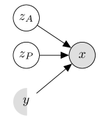
(a) Decoder
(forward model)

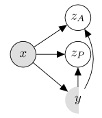
(b) Encoder
(inverse model)

Figure 2: Graphical model representations of (a) the likelihood $p_{\theta}(x|z_{A},z_{P},y)$ and (b) the variational posterior approximation $q_{\phi}(y|x)q_{\phi}(z_{A},z_{P}|x,y)$ of p³VAE. White nodes are latent variables while gray ones are observed variables. Note that $y$ can be either observed or not.

We assume that a data point $x\in\mathcal{X}$ is generated by a random process that involves continuous latent variables $z_{A}\in\mathcal{Z}_{A}$ and $z_{P}\in\mathcal{Z}_{P}$ as well as discrete variables $y\in\mathcal{Y}$ that are sometimes observed, and sometimes unobserved. We assume that the latent variable $z_{P}$ is grounded to some physical properties while the latent variable $z_{A}$ has no physical meaning. $z_{P}$ could be, for instance, the pixel-wise irradiance mentioned in section 1. $y$ is a categorical variable such as the class, for which we have annotations for a few data points. $\mathcal{X}$, $\mathcal{Y}$, $\mathcal{Z}_{A}$ and $\mathcal{Z}_{P}$ are subsets of the euclidean space.

The generative process consists of two steps: (1) values of $z_{A}$, $z_{P}$ and $y$ are generated from a prior distribution $p(z_{A},z_{P},y)$; (2) a value $x$ is generated from the conditional distribution $p_{\theta}(x|z_{A},z_{P},y)$ parameterized by $\theta$. We assume that latent variables $z_{A}$, $z_{P}$, $y$ are independent factors of variations, i.e. that they are mutually independent:

$$p(z_{A},z_{P},y):=p(z_{A})p(z_{P})p(y)$$ (1)

Besides, we assume a Gaussian observation noise $\Sigma$ and define the likelihood as follows:

$$p_{\theta}(x|z_{A},z_{P},y):=\mathcal{N}\big{(}x|f_{P}\circ f_{A}(z_{A},z_{P},y),\Sigma\big{)}$$ (2)

where $f_{A}:\mathcal{Z}_{A}\times\mathcal{Y}\longrightarrow\mathcal{X}$ is a neural network and $f_{P}:\mathcal{Z}_{P}\times\mathcal{X}\longrightarrow\mathcal{X}$ is a physics model differentiable with regard to its inputs.

We would like to maximize the marginal likelihood $p_{\theta}(x,y)$ when $y$ is observed and $p_{\theta}(x)$ otherwise, which are unfortunately intractable. Therefore, we follow the state-of-the-art variational optimization technique introduced in [8] by approximating the true posterior $p_{\theta}(z_{A},z_{P},y|x)$ by a recognition model $q_{\phi}(z_{A},z_{P},y|x)$. Furthermore, we assume that $q_{\phi}(z_{A},z_{P}|x,y)$ factorizes as follows:

$$q_{\phi}(z_{A},z_{P}|x,y):=q_{\phi}(z_{A}|x,y)q_{\phi}(z_{P}|x,y)$$ (3)

The encoding part $q_{\phi}(z_{A},z_{P},y|x)$ and the decoding part $p_{\theta}(x|z_{A},z_{P},y)$ form a variational autoencoder (with parameters $\theta$ and $\phi$).

3.1.2 p³VAE semi-supervised training

We now explain how we adapted the semi-supervised optimization scheme introduced by [16] to the training of our model.

Semi-supervised Model Objective. The objective function derived by [16] for an observation $x$ is twofold. First, when its label $y$ is observed, the evidence lower bound of the marginal log-likelihood $\mbox{log}\>p_{\theta}(x,y)$ is:

$$\begin{split}-\mathcal{L}(x,y)&=\mathbb{E}_{q_{\phi}(z_{A},z_{P}|x,y)}[\mbox{log}\>p_{\theta}(x|z_{A},z_{P},y)+\mbox{log}\>p(y)+\mbox{log}\>p(z_{P},z_{A})-\mbox{log}\>q_{\phi}(z_{A},z_{P}|x,y)]\\ &\leq\mbox{log}\>p_{\theta}(x,y)\end{split}$$ (4)

Second, when the label is not observed, the evidence lower bound of the marginal log-likelihood $\mbox{log}\>p_{\theta}(x)$ is:

$$\begin{split}-\mathcal{U}(x)&=\mathbb{E}_{q_{\phi}(z_{A},z_{P},y|x)}[\mbox{log}\>p_{\theta}(x|z_{A},z_{P},y)+\mbox{log}\>p(y)+\mbox{log}\>p(z_{P},z_{A})-\mbox{log}\>q_{\phi}(z_{A},z_{P},y|x)]\\ &=\sum_{y}q_{\phi}(y|x)\big{(}-\mathcal{L}(x,y)\big{)}+\mathcal{H}\big{(}q_{\phi}(y|x)\big{)}\leq\mbox{log}\>p_{\theta}(x)\end{split}$$ (5)

where $\mathcal{H}\big{(}q_{\phi}(y|x)\big{)}$ denotes the entropy of $y|x$. Besides, we can note that the term $\mathbb{E}_{q_{\phi}(z_{A},z_{P}|x,y)}[\mbox{log}\>p(z_{A},z_{P})-\mbox{log}\>q_{\phi}(z_{A},z_{P}|x,y)]$ in equation (4) is the negative Kullback-Leibler divergence between $q_{\phi}(z_{A},z_{P}|x,y)$ and $p(z_{A},z_{P})$.

The categorical predictive distribution $q_{\phi}(y|x)$ only contributes in the second objective function (5). To remedy this, [16] adds a classification loss to the total objective function, so that $q_{\phi}(y|x)$ also learns from labeled data. The final objective function is defined as follows:

$$\mathcal{J}:=\sum_{x,y\sim\tilde{p}_{l}}\big{[}\mathcal{L}(x,y)-\alpha\>\mbox{log}\>q_{\phi}(y|x)\big{]}+\sum_{x\sim\tilde{p}_{u}}\mathcal{U}(x)$$ (6)

where $\tilde{p}_{l}$ and $\tilde{p}_{u}$ are the empirical labeled and unlabeled data distribution, respectively, and $\alpha$ is a hyper-parameter that controls the relative weight between generative and purely discriminative learning.

Gradient stopping. Our contribution to the semi-supervised optimization scheme is what we refer as gradient stopping. The machine learning model $f_{A}$ generates data features from the categorical variable $y$ and the continuous variable $z_{A}$. Because $f_{A}$ has very poor extrapolation capabilities, some inconsistent values of $(z_{A},z_{P},y)$ can lead to a good reconstruction of the training data. To mitigate this issue, we do not back-propagate the gradients with regard to $f_{A}$ parameters when $y$ is not observed.

3.1.3 Inference

At inference, [16] uses the approximate predictive distribution $q_{\phi}(y|x)$ to make predictions. However, although the true predictive distribution $p_{\theta}(y|x)$ is intractable, we can compute $\operatorname*{arg\,max}_{y}p_{\theta}(y|x)$ if we are only interested in the class predictions. As a matter of fact, assuming that $p(y)$ is uniform, we have from Bayes rule that:

$$p_{\theta}(y|x)=\frac{p_{\theta}(x|y)p(y)}{p_{\theta}(x)}\propto p_{\theta}(x|y)$$ (7)

Moreover, denoting $[z_{A}\>z_{P}]$ as $z$, which is independent from $y$, we can write that:

$$p_{\theta}(x|y) =\int p_{\theta}(x,z|y)\>dz=\int p_{\theta}(x|y,z)p(z)\>dz=\mathbb{E}_{z\sim p(z)}p_{\theta}(x|y,z)$$ (8)

Thus, we can perform Monte Carlo sampling to estimate $p_{\theta}(x|y)$. In order to decrease the variance of the estimation, we can sample $z$ from $q_{\phi}(z|x)$, performing importance sampling as follows:

$$p_{\theta}(x|y) =\mathbb{E}_{z\sim q_{\phi}(z|x)}\frac{p(z)}{q_{\phi}(z|x)}p_{\theta}(x|y,z)=\mathbb{E}_{y^{\ast}\sim q_{\phi}(y|x)}\mathbb{E}_{z\sim q_{\phi}(z|x,y^{\ast})}\frac{p(z)}{q_{\phi}(z|x)}p_{\theta}(x|y,z)$$ (9)

To our knowledge, this derivation of $\operatorname*{arg\,max}_{y}p_{\theta}(y|x)$ has not yet been used in the context of semi-supervised VAEs, while it is close to the importance sampling technique introduced in [40] to estimate the marginal likelihood of VAEs. Besides, this derivation offers a convenient way to estimate the uncertainty over the inferred latent variables. We can easily compute the empirical standard deviation of the $z^{i}$s where $z^{i}\sim q_{\phi}(z|x,y^{\ast})$ and $y^{\ast}\sim q_{\phi}(y|x)$.

3.2 Application of the model to optical remote sensing data

In this section, we apply our methodology to the pixel-wise classification of airborne hyperspectral images. We first describe the physical model and then introduce the design of the VAE.

3.2.1 The radiative transfer model

Remote sensing optical sensors measure spectral radiance, i.e. a radiant flux per unit solid angle, per unit projected area, per unit wavelength (W.sr^-1.m^-2.nm^-1). Spectral radiance, in the reflective domain, is dependant of sun irradiance, of the atmospheric composition as well as the land cover and comes from various sources (see the illustration of irradiance and radiance terms on fig. 3). In contrast, reflectance, that is the ratio of the reflected radiant flux on the incident radiant flux, only depends on matter chemical composition. Therefore, reflectance is a much more relevant feature for classification. Atmospheric corrections code, such as COCHISE [41], aim to deduct the atmospheric contribution to the measured radiance and to estimate pixel-wise reflectance. In the following, we introduce the basics of radiative transfer on which atmospheric codes are based on. In particular, we will focus on hypothesis that yield poor reflectance estimates when they do not hold true.

As most atmospheric codes do, we assume that land surfaces are lambertian, i.e. that they reflect radiation isotropically. We express the reflectance, as it is commonly done in the literature, at wavelength $\lambda$ of a pixel of coordinates $(x,y)$ as $\rho^{xy\lambda}$:

$$\rho^{xy\lambda} =\frac{\pi R_{dir}^{xy\lambda}}{I_{tot}^{xy\lambda}\tau_{dir}^{\lambda}} \mbox{with}\left\{\begin{array}[]{ll}R_{dir}^{xy\lambda}&=R_{tot}^{xy\lambda}-R_{env}^{xy\lambda}-R_{atm}^{\lambda}\\ &\\ I_{tot}^{xy\lambda}&=I_{dir}^{xy\lambda}+I_{dif}^{xy\lambda}+I_{coup}^{xy\lambda}+I_{refl}^{xy\lambda}\end{array}\right.$$ (13)

where (leaving the dependence to $x,y$ and $\lambda$ implicit):

• $R_{tot}$ is the radiance measured by the sensor,

• $R_{atm}$ is the portion of $R_{tot}$ that is scattered by the atmosphere without any interactions with the ground,

• $R_{env}$ is the portion of $R_{tot}$ that comes from the neighbourhood of the pixel,

• $R_{dir}$ is the portion of $R_{tot}$ that comes from the pixel,

• $I_{dir}$ is the irradiance directly coming from the sun,

• $I_{dif}$ is the irradiance scattered by the atmosphere,

• $I_{coup}$ is the irradiance coming from the coupling between the ground and the atmosphere,

• $I_{refl}$ is the irradiance coming from neighbouring 3D structures.

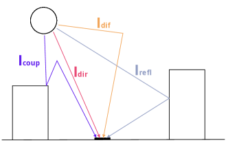
(a) Irradiance terms

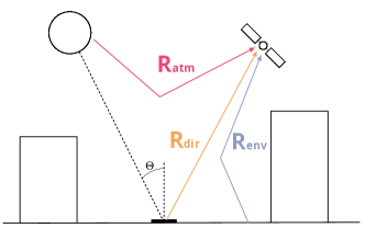
(b) Radiance terms

Figure 3: Illustration of the radiative components described in section 3.2.1. Figure reproduced from [42].

Those terms are illustrated on Fig. 3. More precisely,

$$I_{dir}=\delta_{dir}\cdot cos\>\Theta\cdot I_{dir}^{o}$$ (14)

where $\delta_{dir}$ is the portion of pixel directly lit by sun, $\Theta$ is the solar incidence angle (i.e. the angle between the sun direction and the local normal) and $I_{dir}^{o}$ is the direct irradiance for $\delta_{dir}=1$ and $\Theta=0$. $I_{dif}$ can be approximated by:

$$I_{dif}=\Omega\cdot p_{\Theta}\cdot I_{dif}^{o}$$ (15)

where $\Omega$ is the sky viewing angle factor, $p_{\Theta}$ is a correction coefficient that accounts for the anisotropy of the diffuse irradiance and $I_{dif}^{o}$ is the diffuse irradiance for a pixel on a horizontal ground with $\Omega=1$ (i.e. a full half sphere). As a matter of fact, the diffuse irradiance near the sun direction is much higher than the diffuse irradiance from directions further away from the sun. Thus, the true diffuse irradiance depends on the part of the sky observed from the pixel point of view.

Atmospheric codes that do not need a digital surface model (topography and buildings data) such as COCHISE [41] make the hypothesis that the ground is flat: $\Theta=\Theta^{o}$ (the solar zenith angle), $\delta_{dir}=1$ (there are no shadows), and $\Omega=1$ (each pixel sees the entire sky). Accordingly, pixels on a slope or in shadows will have poor reflectance estimates. More precisely, if we neglect the contributions of $I_{coupl}$ and $I_{refl}$, we can easily derive the ratio between the estimated reflectance $\rho$ and the true reflectance $\rho^{\ast}$ for a given wavelength, as a function of the true local parameters $\delta_{dir}^{\ast}$, $\Theta^{\ast}$, $\Omega^{\ast}$ and $p_{\Theta}^{\ast}$:

$$\frac{\rho}{\rho^{\ast}}=\frac{\delta_{dir}^{\ast}\cdot cos\>\Theta^{\ast}\cdot I_{dir}^{o}+\Omega^{\ast}\cdot p_{\Theta}^{\ast}\cdot I_{dif}^{o}}{cos\>\Theta^{o}\cdot I_{dir}^{o}+I_{dif}^{o}}$$ (16)

This ratio is the deductive bias that we introduce in the decoding part of p³VAE. It is a strong assumption on how the signal behaves under local irradiance conditions. Here we emphasize the fact that the ratio depends on the wavelength $\lambda$ and that it is non-linear with regard to $\delta_{dir}^{\ast}$, $cos\>\Theta^{\ast}$, $\Omega^{\ast}$ and $p_{\Theta}^{\ast}$, as illustrated on Fig. 4. We argue that this behaviour could hardly be modeled by a neural network that would likely fall in local optima.

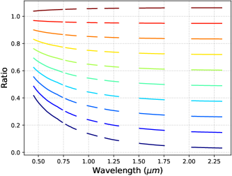
(a) $I_{dif}=I_{dif}^{o}$, $\delta_{dir}\in\mbox{[}0,1\mbox{]}$

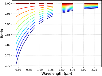
(b) $I_{dir}=I_{dir}^{o}$, $\Omega\in\mbox{[}0.3,1\mbox{]}$

Figure 4: Ratio of the estimated reflectance under the true reflectance for varying irradiance conditions. Blue lines correspond to low values and red lines to high values of (a) $\delta_{dir}$ and (b) $\Omega$. The a priori knowledge expressed by this ratio is explicitly used in the layers of our generative model, as described in section 3.2.2.

3.2.2 Integrating the radiative transfer model into p³VAE

In this section, we explain how we integrate the radiative transfer model into p³VAE and specifically motivate the modeling of the latent variables, encoder, and decoder.

$\blacksquare$ Latent variables and priors

Reflectance intra-class variability does not only come from local irradiance conditions. One semantic land cover class gathers many different materials. For instance, a vegetation class would gather, on one hand, various tree species with different reflectance spectra, and on the other hand, individuals from the same specie with different bio-physical properties (such as water or chlorophyll content). We refer to this variability as intrinsic intra-class variability. Therefore, the key challenge of our hybrid model is to distinguish the intrinsic variability from the irradiance-based variability in order to better predict the class. To this end, we define the latent variables as follows.

The class of a pixel is modeled by the categorical variable $y\in\{1,\ldots,C\}$. In order to model the intrinsic and irradiance-based intra-class variabilities, we considered two latent variables, $z_{A}$ and $z_{P}$, respectively. Following the radiative transfer model we derived above, we expect $z_{P}$ to approximate $\delta_{dir}$, $cos\>\Theta$, $\Omega$ and $p_{\Theta}$. Although, inferring a four dimensional latent variable grounded to $\delta_{dir}$, $cos\>\Theta$, $\Omega$ and $p_{\Theta}$ at the same time led to poor local optima, we constrained the latent space as follows:

$$\delta_{dir}cos\>\Theta \leftarrow z_{P}$$ (17)

$$\Omega\>p_{\Theta} \leftarrow g(z_{P})$$ (18)

where $g$ is an empirical function that will be discussed in section 5.2. Since $\delta_{dir}\in[0,1]$ and $cos\>\Theta\in[0,1]$, $z_{P}$ should lie in $[0,1]$. For this reason and because we would like a flexible distribution to model $z_{P}$, we chose a Beta distribution.

The latent variable $z_{A}$ is not grounded to a physical quantity. However, we could interpret $z_{A}$ as the different reflectance spectra one class could take (e.g. different tree species). Thus, we modeled $z_{A}$ with a Dirichlet distribution of dimension $n_{A}$ which values can be interpreted as a distribution probability or as the abundance of different subclasses.

Prior distributions are defined as follows:

$$p(y) :=\mathcal{U}(\{1,\ldots,C\}); p(z_{P}) :=Beta(z_{P}|\alpha^{o},\beta^{o}); p(z_{A}) :=Dir(z_{P}|\gamma^{o})$$ (19)

We empirically set $\alpha^{o}$ to $1$ and $\beta^{o}=\frac{1-\cos\>\Theta^{o}}{\cos\>\Theta^{o}+\epsilon}\alpha^{o}$ where $\epsilon$ is a small constant to avoid division by zero and $\Theta^{o}$ is the solar incidence angle. This prior distribution favors high values of $z_{P}$ while $\mathbb{E}_{p(z_{P})}z_{P}=\cos\>\Theta^{o}$, which is what we expect on a flat ground. We set $\gamma^{o}=[1\ldots 1]_{1\times n_{A}}$, which is equivalent to having a uniform prior.

$\blacksquare$ Encoder

The approximated posterior (parameterized by $\phi$), i.e. the encoding part, is defined as follows:

$$q_{\phi}(z_{P},z_{A}|x,y):=q_{\phi}(z_{P}|x,y)q_{\phi}(z_{A}|x,y)$$ (20)

$$q_{\phi}(z_{P}|x,y) :=Beta(z_{P}|\alpha(x,y),\beta(x,y)); q_{\phi}(z_{A}|x,y) :=Dir(z_{A}|\gamma(x,y))$$ (21)

$\alpha$, $\beta$ and $\gamma$ are neural networks that will be described in details in section 5.

$\blacksquare$ Decoder

The decoder has a physical part $f_{P}$ and a statistical part $f_{A}$, parameterized by $\theta$. $f_{A}$ estimates the true reflectance $\hat{\rho}\in[0,1]^{B}$, where $B$ is the spectral dimension, based on the class $y$ and the intrinsic variability $z_{A}$:

$$\begin{split}f_{A}:&\{1,\ldots,C\}\times[0,1]^{n_{A}}\longrightarrow[0,1]^{B}\\ &(y,z_{A})\longmapsto\hat{\rho}=\sum_{k=1}^{n_{A}}z_{A}[k]f^{1}_{A}(y)[k]\end{split}$$ (22)

where $f^{1}_{A}$ is a neural network. $f_{P}$ is a deterministic function derived from the radiative transfer model described in section 3.2.1 that computes the observed reflectance $x\in[0,1]^{B}$ based on $\hat{\rho}$ and $z_{P}$:

$$\begin{split}f_{P}:&[0,1]^{B}\times[0,1]\longrightarrow[0,1]^{B}\\ &(\hat{\rho},z_{P})\longmapsto\frac{z_{P}I_{dir}^{o}+g(z_{P})I_{dif}^{o}}{cos\>\Theta^{o}\cdot I_{dir}^{o}+I_{dif}^{o}}\hat{\rho}\end{split}$$ (23)

In contrast with our general framework, we do not model the decoding part of the VAE with a multivariate normal. Denoting $f_{P}(f_{A}(y,z_{A}),z_{P})$ as $\mu$, we instead define the likelihood as follows:

$$\begin{split}p_{\theta}(x|y,z_{P},z_{A}):=\frac{1}{Z}&\>\mathcal{N}(s|\mu,\sigma^{2}I)\cdot exp\big{(}-\lambda\>arccos(\frac{x^{T}\mu}{\|x\|\|\mu\|})\big{)}\end{split}$$ (24)

where $\sigma$ and $\lambda$ are hyperparameters and $Z$ is a finite constant such that the density integrates to one. We demonstrate in the appendix that such a constant exists. The negative log-likelihood derives as follows:

$$-log\>p_{\theta}(x|y,z_{P},z_{A})= \frac{1}{\sigma^{2}}MSE(x,\mu)+\lambda\>arccos(\frac{x^{T}\mu}{\|x\|\|\mu\|})+C$$ (25)

where C is a constant. Therefore, maximizing the likelihood of the data is equivalent to minimizing a linear combination of the mean squared error and the spectral angle between the observations $x^{(i)}$ and $\mu^{(i)}=f_{P}(f_{A}(y^{(i)},z_{A}^{(i)}),z_{P}^{(i)})$. The other consequence of this additional term in the density is that, without knowing the value of the constant $Z$, we cannot properly evaluate the likelihood for a given data point and neither sample from the likelihood. However, it is not an issue in our case because we are only interested in the predictions of the model.

4 Data

(a)

(b)

(c)

Figure 5: (a) False color composition of the simulated hyperspectral image and its (b) training and (c) validation ground truths.

In this section, we describe the simulated and real data used in our experiments. Simulated data allowed to compute quantitative metrics that were valuable for the results interpretation, as we will see in section 5. Then, a subset of a real hyperspectral image is presented. It allowed us to test our model in a real case that includes physical phenomena not taken into account in the simulations, such as non-lambertian materials, Earth-atmosphere coupling and the neighbouring contribution.

4.1 Simulated data

We simulated an airborne hyperspectral image with the radiative transfer software DART [43]. 300 spectral bands with a $6.5$ nm resolution and a $0.5$ m ground sampling distance were simulated, without simulating the Earth-atmosphere coupling. A false-color image and its ground truth are shown in Fig. 5. The scene was simulated with five materials (vegetation, sheet metal, sandy loam, tile and asphalt) whose mean reflectance spectra are shown in fig. 5.4.1 (spectra were sampled with a gaussian noise). Some classes gather different materials to have a realistic intrinsic inter-class variability. For instance, the vegetation class has three spectra which correspond to healthy grass, stressed grass and eucalyptus reflectances. We refer to those different materials within one class as subclasses. The azimuth angle is equal to 180 degrees, the solar zenithal angle is equal to 30 degrees and the roofs have different slopes. Moreover, to reproduce the scarcity of annotations in remote sensing, we labeled only a few pixels in the training data set and used the unlabeled pixels in our validation set. In particular, the training data set:

• does not include vegetation, asphalt and sandy loam pixels in the shadows,

• partially includes tile pixels on different slopes,

• contains all pixels of sheet metal.

Simulating a scene was very convenient as we precisely knew the topography and the reflectance of each material. To test our model, we computed roughly $10,000$ test spectra per class with different slopes, direct irradiance and sky viewing angle. We also made different combinations of reflectance spectra within each class. Precisely, the factors that were used to generate a spectra $x$ were the class $y$, the portion of direct irradiance $\delta_{dir}$, the solar incidence angle $\Theta$, the sky viewing angle factor $\Omega$, the anisotropy correction coefficient $p_{\Theta}$, the intra-class mixing coefficient $\alpha\in[0,1]$ and the subclass configuration $\eta$:

$$\begin{split}x=&\frac{\delta_{dir}cos\>\Theta I_{dir}^{o}+\Omega\>p_{\Theta}I_{dif}^{o}}{cos\>\Theta^{o}\cdot I_{dir}^{o}+I_{dif}^{o}}\tilde{\rho}\\ \end{split}$$ (26)

with:

$$\tilde{\rho}=\alpha\rho[y][\eta_{1}]+(1-\alpha)\rho[y][\eta_{2}]$$ (27)

where $\rho[y][\eta_{i}]$ denotes the reflectance spectrum of the $\eta_{i}$th subclass of class $y$.

For the test data set, the simulation of spectra rather than images was very convenient to cover the whole range of variation factors.

4.2 Real data

We used subsets of the recently published airborne hyperspectral data set of the CAMCATT-AI4GEO experiment in Toulouse, France [44]. Data was acquired with a AisaFENIX 1K camera, which covers the spectral range from 0.4 µm to 2.5 µm with a 1 m ground sampling distance. Data was converted in radiance at aircraft level through radiometric and geometric corrections. Then, the radiance image was converted to surface reflectance with the atmospheric correction algorithm COCHISE [41] (that makes a flat surface assumption). We labeled a ground truth through a field campaign and photo interpretation. We selected eight land cover classes (Tile, Asphalt, Vegetation, Painted sheet metal, Water, Gravels, Metal and Fiber cement) which were spatially split in a labeled training set, an unlabeled training set and a test set (spectra are shown on fig. 10 in the appendix). The labeled training set, unlabeled training set and test set contain 3671 pixels, 7762 pixels and 10333 pixels, respectively.

5 Experiments

We compared our model, p³VAE, with a conventional CNN [45] (Convolutional Neural Network), a conventional semi-supervised gaussian VAE [16], a semi-supervised InfoGAN [37] and a physics-guided VAE, a variant of p³VAE. On real data, we also tested a semi-supervised version of FG-UNET [46], a deep FCN designed for the semantic segmentation of remote sensing images. Models were optimized and tested on the data sets described in section 4. In this section, we broadly present the architecture of the models (although exhaustive details are in the appendix), present the optimization details, the metrics and the results.

5.1 Models architectures

p³VAE. As seen in section 3.2, the parameters of the posterior distributions $q_{\phi}(z_{P}|x,y)$ and $q_{\phi}(z_{A}|x,y)$ are computed with neural networks $\alpha$, $\beta$ and $\gamma$. $\alpha$ and $\beta$ are dense neural networks because we believe that $z_{P}$ can be inferred only with affine transformations of $x$ and $y$. As far as $z_{A}$ is more related to the shape of $x$, we found more relevant to model $\gamma$ by a convolutional neural network. Concerning the decoder, $f_{A}^{1}$ is the element-wise multiplication of two $B\times n_{A}$ matrices computed with dense neural networks. The approximate predictive distribution $q_{\phi}(y|x)$ is computed with a convolutional neural network that has rigorously the same architecture than the CNN model described below. The model is trained using gradient stopping as described in section 3.1.2.

CNN. The CNN architecture is very similar to conventional CNNs used in the hyperspectral literature [45]. It is composed of two spectral convolutions (with one kernel per continuous spectral domain), a skip connection and a max-pooling layer, followed by fully connected layers.

Gaussian VAE. We used a conventional semi-supervised gaussian VAE [16]. The encoder of the gausian VAE uses the same convolutional neural network used in the encoder of p³VAE. The dimension of the latent variable $z$ is equal to dim($z_{A}$) $+$ dim($z_{P}$). The decoder is composed of dense layers and a final sigmoid activation.

ssInfoGAN. We followed the technique introduced in [37] to guide an InfoGAN model [38] with semi-supervision. The generator and the discriminator head of the semi-supervised InfoGAN are dense neural networks. The generator takes inputs of size dim($z_{A}$) $+$ dim($z_{P}$) $+$ dim($z$), where $z$ is the incompressible noise (see [38] for exhaustive details on the InfoGAN model). The neural network that computes the auxiliary distribution for the categorical latent code has the same architecture than the dense layers in the CNN above. The neural network that computes the auxiliary distribution for the continuous latent code is a dense neural network.

FG-UNET. FG-UNET [46] enhances a classical U-net [47] for remote sensing images. In particular, a pixel-wise fully connected path is added to improve the geometric consistency of the predictions to deal with sparse annotations [46]. The encoding part of FG-UNET is composed of five spatial-spectral convolutional layers with two max-pooling operations in-between. The decoding part is composed of five transposed convolutional layers with two up-sampling operations in-between.

Physics-guided VAE. In order to compare the benefits of the physics model only, we designed a physics-guided VAE which encoder and decoder have the same architectures that the ones of p³VAE. The only difference is that the decoder has only a machine learning part $f_{A}$. The model is trained using gradient stopping as described in section 3.1.2.

Every classifiers are turned into bayesian classifiers using MC Dropout [48].

5.2 Optimization

The CNN and the VAE-like models were optimized with the Adam stochastic descent gradient algorithm [49] for 100 and 50 epochs on the simulated and real data, respectively, and a batch size of 64. We optimized ssInfoGAN in the Wasserstein training fashion [50] with the gradient penalty loss introduced in [51], using the RMSProp algorithm for 200 and 150 epochs on the simulated and real data, respectively, and a batch size of 64. FG-UNET was trained with the Adam algorithm for 500 epochs and a batch size of 16. In [46], FG-UNET is optimized by minimizing a standard cross-entropy between labels and predictions. In our experiments, we add an unsupervised reconstruction loss on the L1 norm like in [34] to guide the training of FG-UNET with unlabeled pixels. We tuned the learning rate between $5\cdot 10^{-5}$ and $1\cdot 10^{-4}$ to reach loss convergence on the training and validation sets. We modeled p³VAE empirical function $g:z_{P}\longmapsto\Omega\>p_{\Theta}$ by an affine transformation and tuned its parameters on the validation set. We retained $g(z_{P})=z_{P}+0.2$, which led to good spectral reconstruction under low direct irradiance conditions despite being very simplistic. We weighted the Kullback-Leibler divergence term in equations (4) and (5) by $\beta=10^{-4}$ following [10] technique. We also weighted the entropy term in equation (5) to balance between high accuracy and high uncertainty with a $10^{-1}$ coefficient. Besides, we applied a Ridge regularization on the weights of the classifiers and encoders with a $10^{-2}$ penalty coefficient.

5.3 Metrics

We computed the widely used F1 score for each class, which reflects the performance of the models on the pixel-wise classification task, as well as the JEMMIG metric [52] (for simulated data only) that measures disentanglement. A latent space is said to be disentangled if its variables independently capture true underlying factors that explain the data [53]. Assessing whether a representation is disentangled is still an active research topic. Nevertheless, [53] made a review of state-of-the art metrics to measure disentanglement, that they decompose in modularity, compactness and explicitness. Modularity guarantees that a variation in one factor only affects a subspace of the latent space, and that this subspace is only affected by one factor. Compactness relates to the size of the subspace affected by the variation in one factor. Finally, explicitness expresses how explicit is the relation between the latent code and the factors. [53] compared thirteen disentanglement metrics, from which we chose the JEMMIG (Joint Entropy Minus Mutual Information Gap) metric because it measures modularity, compactness and explicitness at the same time, and relies on few hyper-parameters.

The JEMMIG metric is computed based on a data set of factors (e.g. categorical classes, local irradiance conditions, etc. described in section 4) and latent codes (the latent representation inferred by the generative models based on the reflectance spectra generated from the factors). In the following, we denote $v$ as the factors and $z$ as the latent code. JEMMIG estimates the mutual information between factors and latent codes. It enhances the MIG (Mutual Information Gap) metric [54]. Intuitively, the mutual information $I(v,z)$ between $v$ and $z$ indicates how much information we have about $z$ when we know $v$. Therefore, the mutual information between a factor $v_{i}$ (e.g. $\delta_{dir}cos\>\Theta$) and its related subspace $z_{\mathcal{K}}$ (e.g. $z_{P}$) should be high while the mutual information between $v_{i}$ and other subspaces should be low. JEMMIG computes the mutual information between each code and factor $I(v_{i},z_{j})$ and retains the two latent variables $z_{\ast}$ and $z_{\circ}$ with the highest mutual information $I(v_{i},z_{\ast})$ and $I(v_{i},z_{\circ})$. The difference between $I(v_{i},z_{\ast})$ and $I(v_{i},z_{\circ})$ reflects how much information related to the factor $v_{i}$ is expressed by $z_{\ast}$ only. Conversely, $z_{\ast}$ could contain information about other factors than $v_{i}$. Thus, to account for the modularity property, JEMMIG also computes the joint entropy $H(v_{i},z_{\ast})$ between $v_{i}$ and $z_{\ast}$, resulting in the following metric:

$$JEMMIG:=H(v_{i},z_{\ast})-\big{(}I(v_{i},z_{\ast})-I(v_{i},z_{\circ})\big{)}$$ (28)

We report the joint entropy and the mutual information gap individually, since, on the one hand, they measure two different properties, and on the other hand, they scale differently. In addition, we report a normalized version of the JEMMIG metric introduced in [53] that scales between $0$ and $1$, the higher being the better.

5.4 Results - simulated data

5.4.1 Accuracy metrics

F1 score. Mean F1 score per class over 10 runs is shown on table 1. First, all semi-supervised models outperformed the fully supervised CNN in terms of average F1 score by a margin of at least 4%. Second, using $q_{\phi}(y|x)$ to make the predictions, semi-supervised models had small differences in term of F1 score, except for ssInfoGAN. Third, making predictions using $\operatorname*{arg\,max}_{y}p_{\theta}(y|x)$, large gains were obtained with the gaussian VAE and p³VAE over the conventional CNN. In particular, p³VAE made significant improvements over the gaussian VAE (+3%), the physics-guided VAE (+9%) and the CNN (+13%). A statistical hypothesis test shows that the average F1 score of the gaussian VAE and p³VAE are significantly different: we reject the hypothesis of equal average with a $0.3\%$ p-value. Even with exhaustive annotations (we added the labels of the "unlabeled" pixels in the training data set and we refer to this setting as full annotations in table 1), p³VAE outperformed the CNN by a 7% margin. Besides, we can notice that the accuracy for Sheet metal, which is the only class with homogoneous irradiance on the training image, is barely the same for every models when $q_{\phi}(y|x)$ is used. Finally, better predictions were made when computing $\operatorname*{arg\,max}_{y}p_{\theta}(y|x)$ except for the physics-guided VAE while ssInfoGAN performed poorly with a 3% lower F1 score than the CNN.

Local irradiance estimate. Fig. 5.4.1 shows, for each class, the inferred $z_{P}$ by p³VAE against the true $\delta_{dir}cos\>\Theta$ of the test data set. Correctly classified pixels are shown as purple points while wrongly predicted pixels are shown as orange points. The size of the points is proportional to the exponential of the empirical standard deviation of $z_{P}$. First, we notice that most confusions are made when $\delta_{dir}cos\>\Theta$ is poorly estimated or when its true value is low. Secondly, we see that most confusions go hand in hand with high $z_{P}$ uncertainty estimates, meaning that two classes are likely, but under very different irradiance conditions. Finally, we see that there is a bias, in the sense that the average prediction of $\delta_{dir}cos\>\Theta$ is different from its true value. $\delta_{dir}cos\>\Theta$ is mostly under-estimated, which is the counterpart of over-estimated reflectance spectra as shown in Fig. 5.4.1 and commented below.

Estimated reflectance. Fig. 5.4.1 shows the estimated reflectance spectra by p³VAE. There are four estimated spectra per class as we set $n_{A}=4$ in our experiments. p³VAE rather well estimated the shape of the spectra. For instance, the absorption peak of clay at 2.2 µm is reconstructed by p³VAE for the classes Tile and Sandy loam. However, the intensity of the spectra is not accurate, which is a consequence of the bias in the $\delta_{dir}cos\>\Theta$ prediction. Finally, we highlight that p³VAE inferred realistic reflectance spectra whereas the estimated spectra by the physics-guided VAE look like white noise as shown in Fig. 5.4.1.

Table 1: Mean F1 score per class over 10 runs

		Classes
Inference model		Vegetation	Sheet metal	Sandy loam	Tile	Asphalt	Average
CNN	$q_{\phi}(y|x)$	0.90	0.81	0.77	0.79	0.75	0.80
	$q_{\phi}(y|x)$ (full annotations)	0.92	0.79	0.90	0.87	0.86	0.86
ssInfoGAN	$q_{\phi}(y|x)$	0.86	0.79	0.75	0.75	0.69	0.77
Gaussian VAE	$q_{\phi}(y|x)$	0.93	0.80	0.87	0.86	0.74	0.84
	$\operatorname*{arg\,max}_{y}p_{\theta}(y|x)$	0.94	0.88	0.90	0.92	0.85	0.90
Physics-guided VAE	$q_{\phi}(y|x)$	0.93	0.81	0.86	0.86	0.76	0.84
	$\operatorname*{arg\,max}_{y}p_{\theta}(y|x)$	0.86	0.85	0.83	0.75	0.77	0.81
p3VAE	$q_{\phi}(y|x)$	0.92	0.82	0.88	0.87	0.81	0.86
	$\operatorname*{arg\,max}_{y}p_{\theta}(y|x)$	0.96	0.97	0.90	0.90	0.93	0.93

¹The CNN was optimized with every pixels labeled on the image (i.e. the labeled and unlabeled sets showed on Fig. 5), in contrast with every other cases where the image is partially labeled.

Table 2: Mean JEMMIG metric over 10 runs

		Factors
Metric	Model	$y$	$\delta_{dir}cos\>\Theta$	$\Omega p_{\Theta}$	$\alpha$	$\eta$	Average
Joint entropy ($\downarrow$)	Gaussian VAE	2.8	6.9	6.9	4.5	4.5	5.1
	Physics-guided VAE	3.1	6.4	6.0	4.4	4.4	4.9
	ssInfoGAN	3.2	6.3	5.4	4.5	4.5	4.8
	p3VAE	2.7	7.3	7.2	4.4	4.4	5.2
Mutual information gap ($\uparrow$)	Gaussian VAE	0.62	0.18	0.096	0.20	0.20	0.26
	Physics-guided VAE	1.0	0.068	0.021	0.28	0.28	0.33
	ssInfoGAN	0.92	0.16	0.040	0.29	0.29	0.34
	p3VAE	1.2	0.85	0.012	0.31	0.31	0.54
Normalized JEMMIG score ($\uparrow$)	Gaussian VAE	0.67	0.22	0.12	0.39	0.39	0.36
	Physics-guided VAE	0.69	0.26	0.21	0.42	0.42	0.40
	ssInfoGAN	0.66	0.28	0.29	0.41	0.41	0.41
	p3VAE	0.78	0.25	0.061	0.42	0.42	0.38

¹($\downarrow$) means that the lower is the better while ($\uparrow$) means that the higher is the better.

figureOn the left column: predicted $z_{P}$ against true $\delta_{dir}cos\>\Theta$ for each class with p³VAE. Each point represents a pixel, which is correctly classified if shown in purple, or wrongly classified if shown in orange. The size of the points is proportional to the exponential of the empirical standard deviation of $z_{P}$. On the right column: Estimated class reflectance for each class with p³VAE. True reflectance spectra, that were used for data simulation, are plotted in dashed black lines.

[] [] [] [] []

figureEstimated class reflectance for (a) vegetation, (b) sheet metal, (c) sandy loam, (d) tile and (e) asphalt with the physics-guided VAE (i.e. the same architecture than p³VAE without the integration of the physical model). True reflectance spectra, that were used for data simulation, are plotted in dashed black lines.

5.4.2 Disentanglement

Table 2 shows the averaged JEMMIG metric for each factor over 10 runs. $y$ is the class of the pixel, $\delta_{dir}cos\>\Theta$ and $\Omega p_{\Theta}$ are the local irradiance conditions, $\alpha$ is the intra-class mixing coefficient and $\eta$ represents the subclasses configuration (see section 4 for more details). First, the best overall joint entropy was reached by ssInfoGAN. Differences of joint entropy for the factors $\alpha$ and $\eta$ are not significant though and the best joint entropy for the class factor was achieved by p³VAE (a statistical hypothesis test shows that p³VAE reached a significantly lower joint entropy than the gaussian VAE with a 0.9% p-value). The same observations can be drawn on the normalized JEMMIG score. In contrast, p³VAE outperformed other models in term of mutual information gap (MIG), except for the $\Omega p_{\Theta}$ factor. Largest discrepancies between the models in term of MIG were observed for the irradiance conditions factors. The best MIG score for the $\delta_{dir}cos\>\Theta$ factor, reached by p³VAE, was more than twice the score reached by ssInfoGAN. In contrast, the MIG for $\Omega p_{\Theta}$ was 8 times lower with p³VAE than the gaussian VAE, although every MIG scores for this factor were near zero.

5.5 Results - real data

5.5.1 Accuracy metrics

F1 score. Mean F1 score per class over 10 runs is showed on table 3. The CNN with exhaustive annotations outperformed every models, including p³VAE by a margin of 1%. Excluding the CNN with exhaustive annotations, p³VAE reached a better F1 score than other models (11%, 8%, 16%, 10% and 2% higher than the CNN, FG-UNET, ssInfoGAN, the gaussian VAE and the physics-guided VAE, respectively, using $q_{\phi}(y|x)$). In contrast with the experiments on the simulated data set, VAE-like models obtained better performances using the predictive distribution $q_{\phi}(y|x)$ rather than $\operatorname*{arg\,max}_{y}p_{\theta}(y|x)$.

Land cover maps. Fig. 6 shows land cover maps produced by the CNN and p³VAE on three test scenes that allow to qualitatively assess the accuracy of the models. We do not have a labeled ground truth of those scenes, which moreover include pixels belonging to classes not represented in the training data set. However, we focus on specific areas for which we know the land cover with confidence. On the first scene, the ground vegetation in the shade between the rows of trees was partially confused with asphalt by the CNN, while p³VAE was correct. On the first and the second scenes, asphalt in the shade of buildings was also partially confused with water by the CNN, while p³VAE was correct. On the third scene, the least lit fiber cement roofs were mainly confused with asphalt and metal by the CNN while p³VAE made much fewer confusions.

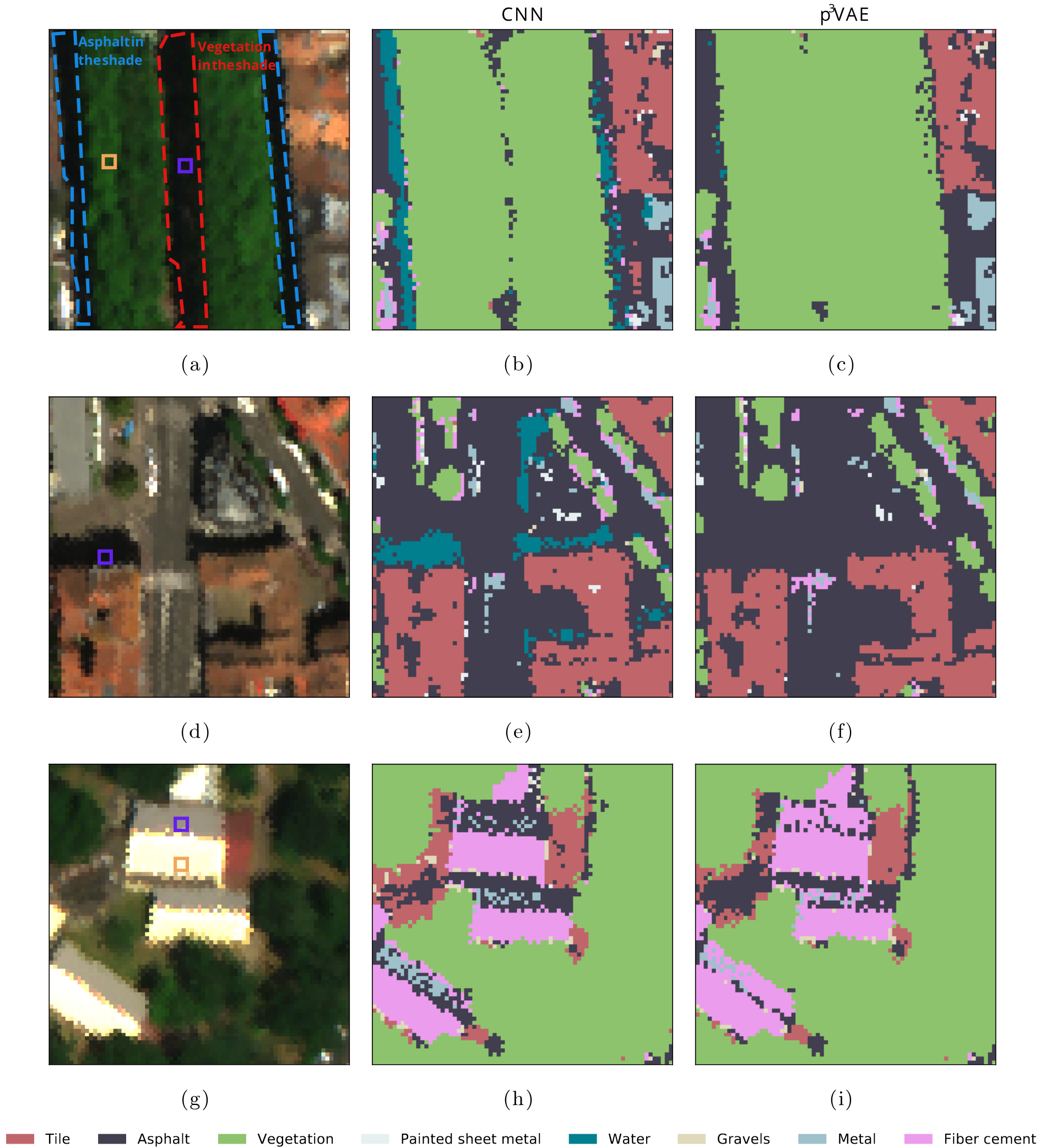
Figure 6: (a)-(d)-(g) False color composition of subsets of the AI4GEO hyperspectral image, (b)-(e)-(h) the predictions of the CNN and (c)-(f)-(i) the predictions of p³VAE.

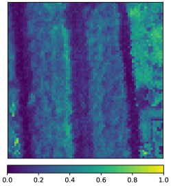
(a)

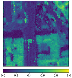
(b)

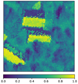
(c)

Figure 7: Latent variable $z_{P}$, predicted by p³VAE on AI4GEO hyperspectral images, which corresponds to the normalized direct irradiance.

5.5.2 Disentanglement

Qualitative assessment of $\boldsymbol{z_{P}}$ interpretability. We can observe on Fig. 7 the predicted latent variable $z_{P}$ over the scenes. Relative differences of $z_{P}$ values within one material under different irradiance conditions are consistent. For instance, pixels on roofs that faces the sun (under high direct irradiance) have high values of $z_{P}$ while pixels on roofs in the other direction (under low direct irradiance) have low values of $z_{P}$. However, we also observe that different materials with the same irradiance conditions can have different $z_{P}$ values. For instance, pixels on the road and pixels on flat roofs (that roughly have the same direct irradiance) have different $z_{P}$ values.

5.6 Ablation study

Table 3: Mean F1 score per class over 10 runs

		Classes
Inference model		#1	#2	#3	#4	#5	#6	#7	#8	Average
CNN	$q_{\phi}(y|x)$	0.92	0.41	0.91	0.92	0.83	0.89	0.87	0.56	0.79
	$q_{\phi}(y|x)$ (full annotations)	0.96	0.53	0.98	1.00	0.99	0.98	0.99	0.87	0.91
FG-Unet	$q_{\phi}(y|x)$	0.94	0.50	0.87	0.97	0.54	0.98	0.92	0.83	0.82
ssInfoGAN	$q_{\phi}(y|x)$	0.86	0.34	0.78	0.95	0.40	0.94	0.91	0.76	0.74
Gaussian VAE	$q_{\phi}(y|x)$	0.94	0.27	0.88	0.96	0.83	0.92	0.96	0.66	0.80
	$\operatorname*{arg\,max}_{y}p_{\theta}(y|x)$	0.82	0.40	0.86	0.73	0.84	0.60	0.79	0.63	0.71
Physics-guided VAE	$q_{\phi}(y|x)$	0.95	0.48	0.97	1.00	0.98	0.98	0.87	0.78	0.88
	$\operatorname*{arg\,max}_{y}p_{\theta}(y|x)$	0.92	0.48	0.97	0.99	1.00	0.99	0.84	0.78	0.87
p3VAE	$q_{\phi}(y|x)$	0.95	0.51	0.98	0.99	0.98	0.99	0.96	0.81	0.90
	$\operatorname*{arg\,max}_{y}p_{\theta}(y|x)$	0.93	0.49	0.97	0.91	0.99	0.79	0.90	0.78	0.84

¹ #1: Tile, #2: Asphalt, #3: Vegetation, #4: Painted sheet metal, #5: Water, #6: Gravels, #7: Metal, #8: Fiber cement.
² The CNN was optimized with every pixels labeled on the image (i.e. the labeled and unlabeled sets), in contrast with every other cases where the image is partially labeled.

In this section, we study the impact of gradient stopping (described in section 3) on the optimization of p³VAE. Table 5.6 shows the average F1 score of p³VAE optimized with or without gradient stopping on the simulated and real data sets. On simulated data, statistical hypothesis tests show that gradient stopping has not a significant influence on the model performance, for both inference techniques. However, a look at the estimated reflectance spectra by p³VAE without gradient stopping shows that the machine learning part learns unrealistic spectra. For instance, we plot the estimated reflectance spectra of the class asphalt by p³VAE without gradient stopping on Fig. 5.6. Among the four estimated spectra, one is actually similar to a real asphalt spectrum, one is similar to a vegetation spectrum and others do not correspond to any material in the scene. On real data, statistical hypothesis tests show that gradient stopping does have a significant influence on the model performance, for both inference techniques (with a 1.8% p-value for the inference with $q_{\phi}(y|x)$).

tablep³VAE average F1 score Inference technique no gs gs Simulated data set $q_{\boldsymbol{\phi}}(y|x)$ 0.86 0.86 $\operatorname*{arg\,max}_{y}p_{\boldsymbol{\theta}}(y|x)$ 0.92 0.93 Real data set $q_{\boldsymbol{\phi}}(y|x)$ 0.88 0.90 $\operatorname*{arg\,max}_{y}p_{\boldsymbol{\theta}}(y|x)$ 0.73 0.84

¹gs refers to the gradient stopping technique described in section 3.1.2.

figure[Estimated reflectance spectra of the class asphalt by p³VAE without gradient stopping]Estimated reflectance spectra of the class asphalt by p³VAE without gradient stopping. Only spectrum is actually similar to a spectrum of asphalt.

6 Discussion

In this section, we discuss the performances of p³VAE against other models, the particularities of its optimization and its relation to $\phi$-VAE. Because our experiments showed that its interpolation capabilities are similar to conventional generative models, we focus on its extrapolation and disentanglement capacities which are greatly increased by its physical part.

6.1 Extrapolation capabilities

p³VAE demonstrated high extrapolation capabilities in our experiments. On the simulated data set, great improvements over state-of-the-art models were made by computing predictions with $\operatorname*{arg\,max}_{y}p(y|x)$ (as described in section 3.1.3). As a matter of fact, the physics part $f_{P}$ is explicitly used in this case. In contrast, the physics model is only used during optimization when we perform inference with the predictive distribution $q_{\phi}(y|x)$. On the contrary, higher extrapolation performances were observed on the real data set by computing predictions with $q_{\phi}(y|x)$. This is likely due to the higher intrinsic intra-class variability of real data, especially in a urban environment. As a matter of fact, materials are not lambertian in reality and most pixels are not pure (e.g. asphalt can be mixed with manhole covers or cars, north-facing roofs can be covered by moss, gravels can be mixed with sparse grass, and so on…). Therefore, there is a shift between the train and the test data distribution caused by intrinsic intra-class variability. As far as those variations of reflectance are not caused by variations in the irradiance conditions and are not captured in the training data set, p³VAE sometimes fails to compute a faithful likelihood $p_{\theta}(x|y,z_{A},z_{P})$, which causes more confusions when we compute predictions with $\operatorname*{arg\,max}_{y}p(y|x)$. Therefore, the less the assumptions under which the model is considered perfect are verified, the less accurate is the inference using $\operatorname*{arg\,max}_{y}p(y|x)$.

Experiments on the simulated data set have shown that the physics part of p³VAE makes a great difference in handling data variations caused by variations in the irradiance conditions. The simulated test data set was generated with out-of-distribution physical factors, i.e. test irradiance conditions out of the range of the training irradiance conditions. In particular, the pixels of sheet metal (both labeled and unlabeled) were only seen under the same irradiance conditions during training. For this reason, the CNN and the conventional semi-supervised models failed to predict sheet metal pixels under roughly 20% of the test irradiance conditions using the predictive distribution. However, predictions from the gaussian VAE using $\operatorname*{arg\,max}_{y}p(y|x)$ approximately reduced by half the confusions over the sheet metal class. Besides, the CNN with exhaustive annotations was still worse than gaussian VAE and p³VAE on the simulated data. This illustrates that generative models as a whole can truly graspe some factors of variation that generalize to out-of-distribution data, in contrast to the predictive distribution only. In particular, the physics part of p³VAE highly increased the extrapolation performances for classes with little inter-class similarities (e.g. only 3% of mistakes for the sheet metal class), since the physics model can extrapolate by nature. The limits of p³VAE are reached when two spectra intrinsically share spectral features, such as tile and sandy loam: the model has similar or slightly smaller accuracy, but higher and more meaningful uncertainty, as discussed below. In that sense, experiments on the real data set seem to show that a discriminative model, such as the CNN, can have a a slightly higher discriminative power when a large labeled data set is available.

The physics-guided VAE made worse predictions with $\operatorname*{arg\,max}_{y}p(y|x)$ than with the predictive distribution on the simulated data. We provide an explanation through the analysis of the JEMMIG metric in the next subsection. Concerning ssInfoGAN, it learned to generate realistic samples but it failed to fully capture both the intrinsic and physics intra-class variabilities, as we can see on fig. 9 in the appendix. In addition, realistic samples do not necessarily imply realistic relationships between samples and classes, despite the mutual information term between samples and latent codes in the ssInfoGAN objective.

Finally, the advantage of FG-UNET with respect to the CNN mainly lies in its spatial regularization property. The land cover maps (see fig. 11 in the appendix) produced by FG-UNET are much more geometrically consistent than the land cover maps of the spectral models.

We can derive an uncertainty estimate $\sigma(z_{P})$ over $\delta_{dir}cos\>\Theta$ from p³VAE, which yields easily explainable predictions. In other words, p³VAE can tell us that different classes are likely, but under different conditions. Uncertainty estimates over latent variables grounded to physical properties are naturally more explainable than uncertainty estimates over abstract variables. From a user perspective, this is a valuable feature. Besides, the entropy of the predictive distribution $H\big{(}q_{\phi}(y|x)\big{)}$ gives a complementary uncertainty estimate. In fact, $H\big{(}q_{\phi}(y|x)\big{)}$ and $\sigma(z_{P})$ poorly correlate ($R^{2}\approx 0.2$ in our experiments), because the classifier is generally uncertain in the shadows although $z_{P}$ is well inferred.

6.2 Disentanglement

We evaluated the disentanglement of the latent space qualitatively and quantitatively (further qualitative comparisons are shown in the appendix for the simulated data set). Qualitatively, p³VAE showed higher disentanglement capabilities than other generative models. The decoder architecture, with the machine learning part and the physical part, naturally induces a disentanglement of the latent space. Generated samples with varying $z_{P}$ values automatically yields physically meaningful variations of spectra. Quantitatively, the JEMMIG metric highlights the rough approximation of the true diffuse irradiance as far as p³VAE estimates the same $\Omega\>p_{\Theta}$ given a $\delta_{dir}cos\>\Theta$ estimate: this is the reason why the mutual information gap is very low for the diffuse irradiance factor $\Omega p_{\Theta}$. In contrast, the mutual information gap for the direct irradiance factor is very high, which highlights the natural disentanglement induced by the physics model which grounds $z_{P}$ to $\delta_{dir}cos\>\Theta$. We believe that the joint entropy term for the direct irradiance factor is large because the bias between the predicted $z_{P}$ and the true $\delta_{dir}cos\>\Theta$ depends on the class, which leads to an unclear relation between the factor and the code when the class $y$ is not known. Concerning the physics-guided VAE and ssInfoGAN, they suffered from mode collapse during our experiments on the simulated data. Concerning the physics-guided VAE, the very low mutual information gap for $\delta_{dir}cos\>\Theta$ shows that the physics-guided VAE failed to capture this factor of variation. As a consequence, the model predicts approximately the same $\delta_{dir}cos\>\Theta$ for any spectrum. This is why it had mediocre performances using $\operatorname*{arg\,max}_{y}p_{\theta}(y|x)$ compared to other generative models. This also explains why the physics-guided VAE had rather low joint entropies for the irradiance factors. Concerning ssInfoGAN, visual inspection of the generated samples (see fig 9 in appendix) corroborates the low joint entropy: the model only learned one mode per class (e.g. it only generated healthy grass samples when conditioned on the Vegetation class and only one type of tile when conditioned on the Tile class). Thus, in the case of mode collapse (which causes a low joint entropy of factors and codes), the JEMMIG metric can be misleading and we argue that the mutual information gap is more relevant in this case.

6.3 Optimization

Loss landscape. In our experiments, we had more trouble to reach convergence with p³VAE than other models. In particular, the training loss for some configurations of weights at initialization systematically diverged, irrespective to the learning rate. We guess that the physics model implicitly constrains the admissible solutions of the machine learning part, which leaves the optimization in a local minima from the beginning, for some specific weight initialization.

Gradient stopping. The ablation study described in 4 showed that gradient stopping can have a significant impact on p³VAE, either on the accuracy of the model, or on the relations it infers between the class labels and the estimated reflectance spectra. On the simulated data, similar performances observed with or without gradient stopping highlight that some values of ($y$, $z_{A}$, $z_{P}$) can lead to good reconstructions even with very bad reflectance estimates. In this case though, p³VAE looses physical sense and interpretability. On the real data set, however, a very large decrease of accuracy was observed (when predictions were made with $\operatorname*{arg\,max}_{y}p(y|x)$) without gradient stopping. We believe that this difference between simulated and real data can be explained by a larger noise and a higher intrinsic intra-class variability on real data: the decider might be more prone to diverge with inconsistent values of $(z_{A},z_{P},y)$. Overall, gradient stopping is crucial to regularize the machine learning part $f_{A}$ of p³VAE.

6.4 Relation to physics-integrated VAEs ($\phi$-VAE)

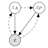
(a) $\phi$-VAE [2]

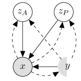
(b) p³VAE (ours)

Figure 8: Graphical model representations of (a) $\phi$-VAE and (b) p³VAE. Solid lines denote the generative model (a) $p_{\theta}(x|z_{A},z_{P})$ and (b) $p_{\theta}(x|z_{A},z_{P},y)$. Dashed lines denote the variational posterior approximation (a) $q_{\phi}(z_{A}|x)q_{\phi}(z_{P}|x,z_{A})$ and (b) $q_{\phi}(y|x)q_{\phi}(z_{A},z_{P}|x,y)$. White nodes are latent variables while gray ones are observed variables. Note that p³VAE is, by nature, a semi-supervised model in contrast to $\phi$-VAE which is unsupervised.

Physics-integrated VAE [2] is, to our knowledge, the first general framework that combines physics models and machine learning models in a variational autoencoder. Our model falls in their formalism as far as $\phi$-VAE latent space is partitioned into two types of data, $z_{A}$ and $z_{P}$ which are inputs of a machine learning model $f_{A}$ and of a physics model $f_{P}$. The differences between $\phi$-VAE and our model, though, are twofold.

Unsupervised VS semi-supervised setting. The first difference, which is minor in architecture, but significant in optimization, is that the latent variables of $\phi$-VAE are never observed. In contrast, we partially observe the discrete variable $y$ of our model during optimization, as we discussed in section 3.1.2.

Imperfect VS perfect physics model. There is a major difference of philosophy between $\phi$-VAE and p³VAE. $\phi$-VAE tackles problems for which an imperfect physics model can approximate the data distribution. In this context, the machine learning part $f_{A}$ of $\phi$-VAE models the residual error of its imperfect physics model $f_{P}$. Intuitively, $z_{A}$ explains the part of the observation $x$ that was not explained by $z_{P}$. This has two practical consequences:

• Firstly, the latent variables $z_{P}$ and $z_{A}$ of $\phi$-VAE are dependent conditioned on $x$:

  $$q_{\phi}(z_{A},z_{P}|x):=q_{\phi}(z_{A}|x)q_{\phi}(z_{P}|x,z_{A})$$ (29)

  In contrast, we assume that $z_{A}$ and $z_{P}$ are independent conditioned on $x$ and $y$.

• Secondly, the expectation of the likelihood $p_{\theta}(x|z_{A},z_{P})$ of $\phi$-VAE is defined as follows:

  $$p_{\theta}(x|z_{P},z_{A}):=\mathcal{N}(x|\mathcal{F}[f_{A},f_{P};z_{P},z_{A}],\Sigma)$$ (30)

  where $\mathcal{F}$ is a functional that evaluates $f_{A}\circ f_{P}$ or solves an equation in the form $f_{A}\circ f_{P}=0$. The notable difference is that the machine learning model of $\phi$-VAE is a function of the physics model output, which is the opposite for our model.

Because the physics part of $\phi$-VAE is imperfect, a specific regularization technique is necessary to control the representation power of the machine learning part. In contrast, our experiments showed that neural networks in p³VAE are less prone to impinge the physics model because they control different subspaces of the latent code.

7 Conclusion

We introduced p³VAE, a hybrid generative model that combines conventional neural networks with a phyics model. In this framework, the assumed perfect physical part partially models the true underlying factors of data variation, which naturally leads to a disentangled latent space and to high extrapolation capabilities. The gradient stopping technique to train p³VAE in a semi-supervised setting led to a good use of the machine learning part, which was reflected with physically meaningful inferred latent variables and uncertainty estimates. The introduced inference technique empirically demonstrated its benefits on a simulated remote sensing scene, showing that high extrapolation performances are reached when the physical model is explicitly used during the inference, provided that the conditions under which the physical model is assumed perfect are verified. In any case, experiments on a real hyperspectral image demonstrated the gains of accuracy p³VAE brings against conventional semi-supervised generative models and supervised convolutional neural networks when few data is labeled.

In future work, we would like to enhance p³VAE to handle spatial context, which we believe could significantly improve the inference of irradiance conditions, though it would bring little discriminating information about the land cover class. We would also like to apply p³VAE to other tasks, such as the quantification of methane emissions with hyperspectral remote sensing data.

Acknowledgments. We thank Pr. Jean Philippe Gastellu-Etchegorry for his precious help handling the DART [43] software.

Appendix

Appendix A Hybrid model likelihood

In section 3.2, we defined the likelihood of our model as follows:

$$p_{\theta}(x|y,z_{P},z_{A}):=\frac{1}{Z}\>f(x)\mathcal{S}(x)$$ (31)

where $f(x)=\mathcal{N}(x|f_{P}(f_{A}(y,z_{A}),z_{P}),\sigma^{2}I)$, $\mathcal{S}(x)=exp\big{(}-\lambda\>arccos(\frac{x^{T}\mu}{\|x\|\|\mu\|})\big{)}$ with $\sigma,\lambda\in\mathbb{R}$ some hyperparameters and $Z$ a finite constant such that the density integrates to one. Let us prove that such a constant $Z:=\int f(x)\cdot\mathcal{S}(x)dx$ exists.

First, we can easily show that $f:[0,1]^{B}\longrightarrow\mathbb{R}$ is square-integrable, as well as $\mathcal{S}:[0,1]^{B}\longrightarrow\mathbb{R}$:

$$\int|\mathcal{S}(x)|^{2}dx =\int_{[0,1]^{B}}exp\big{(}-2\lambda\>arccos(\frac{x^{T}\mu}{\|x\|\|\mu\|})\big{)}dx\leq\int_{[0,1]^{B}}dx=1$$ (32)

since $exp\big{(}-2\lambda\>arccos(\frac{x^{T}\mu}{\|x\|\|\mu\|})\big{)}\leq 1$ for all $\mu$, $x\in[0,1]^{B}$. Moreover, $f$ and $\mathcal{S}$ being continous over $[0,1]^{B}$, the Cauchy-Schwarz inequality implies that:

$$\Bigg{\lvert}\int f(x)\cdot\mathcal{S}(x)dx\Bigg{\rvert} \leq\Bigg{(}\int f(x)^{2}dx\Bigg{)}^{\frac{1}{2}}\Bigg{(}\int\mathcal{S}(x)^{2}dx\Bigg{)}^{\frac{1}{2}}=C\in\mathbb{R}$$ (33)

Thus, $Z\in\mathbb{R}$ and $p_{\theta}(x|y,z_{P},z_{A})$ properly defines a probability density function.

Appendix B Qualitative disentanglement evaluation

A qualitative way to evaluate the disentanglement of the latent space is to plot spectra that maximize the generative model likelihood for different values of the latent variables. Fig. 9 shows the maximum likelihood estimates of the class tile for the physics-guided VAE, p³VAE, the gaussian VAE, and ssInfoGAN. The different estimates were obtained for different realizations of $z_{A}$ and $z_{P}$. $z_{P}$ was interpolated between its lowest and highest values inferred on the training set. $z_{A}$ was interpolated between two values inferred on different types of tile under high and low direct irradiance conditions. We see on Fig. 9 that latent variables $z_{P}$ and $z_{A}$ are disentangled by p³VAE. Firstly, for a given column, the variations of the spectra are only induced by the variation in irradiance conditions : the shape roughly stays the same but the intensity changes. Secondly, for a given row, the variations of the spectra are only induced by the change in the nature of matter : the intensity is the same but the shape changes. In contrast, the physics-guided VAE does not disentangle the latent variables. A variation along one latent variables induces a change both in the irradiance conditions and on the type of tile.

A major difference that we should highlight between the quantitative and qualitative disentanglement evaluation is that the quantitative approach evaluates how a variation of the factors induces a variation of the latent code. The qualitative approach on the other hand evaluates how a change in the latent code induces a change in the observation. Therefore, assessing the disentanglement qualitatively requires expert knowledge.

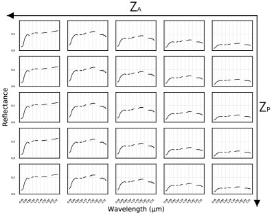
(a) Physics-guided VAE

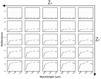
(b) p³VAE

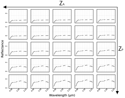
(c) Gaussian VAE

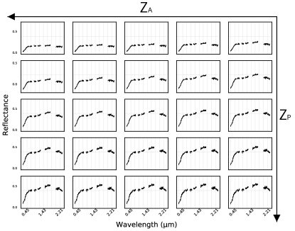
(d) ssInfoGAN

Figure 9: Maximum likelihood estimates of the learned generative models along $z_{P}$ (on the y-axis) and $z_{A}$ (on the x-axis) for the class Tile. $z_{P}$ is interpolated between its minimum (top row) and maximum (bottom row) values inferred on the training data set. $z_{A}$ is interpolated between two realizations of $z_{A}$ that were inferred on two different types of tile of the training set (left and right columns) under high and low direct irradiance conditions, respectively. ssInfoGAN incompressible noise is randomly fixed.

Appendix C Additional data and experiment details

Real labeled spectra of the training labeled set, the training unlabeled set and the test set are shown in Fig. 10. Models architectures are described in Table 4, Table 5, Table 6, Table 7. Additional land cover maps are shown in Fig. 11.

Table 4: Architecture of the CNN

CNN
CNN feature extractor
Input $1\times n_{bands}$
For each continuous spectral segment of length $n$:
$2\times((\lfloor n/5\rfloor)$ 1D conv - ReLU)
Skip connection
$(1\times 2)$ max-pooling
CNN dense classifier
2 $\times$ (FC 256 hidden neurons - ReLU)
FC output layer

Table 5: VAE-like encoders and decoders architectures

Gaussian VAE encoder
Input $1\times n_{bands}$
$(1\times 11)$ 1D conv - ReLU
$(1\times 9)$ 1D conv - ReLU
$(1\times 7)$ 1D conv - ReLU
$(1\times 5)$ 1D conv - ReLU
Concatenation of the class $y$ of size $n_{classes}$
2 $\times$ (FC 256 hidden neurons - ReLU)
FC variational posterior approximation output

Gaussian VAE decoder
Input $1\times(dim(z)+n_{classes})$
2 $\times$ (FC 256 hidden neurons - ReLU)
FC likelihood output

Physics encoder
$z_{P}$ branch
Input $1\times(n_{bands}+n_{classes})$
2 $\times$ (FC 256 hidden neurons - ReLU)
2 $\times$ (FC 256 hidden neurons - ReLU)
FC latent posterior output
$z_{A}$ branch
Input $1\times n_{bands}$
$(1\times 11)$ 1D conv - ReLU
$(1\times 9)$ 1D conv - ReLU
$(1\times 7)$ 1D conv - ReLU
$(1\times 5)$ 1D conv - ReLU
Concatenation of the class $y$ of size $n_{classes}$
2 $\times$ (FC 256 hidden neurons - ReLU)
FC latent posterior output

Physics-guided VAE decoder
Input $1\times n_{classes}$
FC 256 hidden neurons - ReLU	FC 256 hidden neurons - ReLU
FC $n_{bands}$ hidden neurons - Sigmoid	FC $4\times n_{bands}$ hidden neurons - Sigmoid
Element-wise multiplication
Concatenation of $z_{P}$
2 $\times$ (FC 256 hidden neurons - ReLU)
FC likelihood output

p3VAE decoder
Input $1\times n_{classes}$
FC 256 hidden neurons - ReLU	FC 256 hidden neurons - ReLU
FC $n_{bands}$ hidden neurons - Sigmoid	FC $4\times n_{bands}$ hidden neurons - Sigmoid
Element-wise multiplication
Concatenation of $z_{P}$
Evaluation of $f_{P}$

Table 6: ssInfoGAN architecture

GAN discriminator head
Input $1\times n_{bands}$
3 $\times$ (FC 256 hidden neurons - ReLU)
GAN discriminator
Input $1\times 256$
Concatenate the smooth feature
FC 256 hidden neurons

GAN recognition network
Input $1\times 256$
FC 256 hidden neurons - ReLU
FC continuous posterior	CNN dense classifier

GAN generator
Input $1\times(dim(z)+dim(z_{P})+dim(z_{A})+n_{classes})$
3 $\times$ (FC 256 hidden neurons - ReLU)
FC output layer - Sigmoid

Table 7: FG-UNET architecture

Encoder
Input $32\times 32\times n_{bands}$
2 $\times$ ($(3\times 3\times 7)$ 3D conv - stride $(1\times 1\times 3)$ - ReLU)
$\rightarrow$ Features 1
$(2\times 2\times 1)$ max-pooling
2 $\times$ ($(3\times 3\times 7)$ 3D conv - stride 1 - ReLU)
$\rightarrow$ Features 2
$(2\times 2\times 2)$ max-pooling
($(3\times 3\times 7)$ 3D conv - stride 1 - ReLU)

Decoder
Input $4\times 4\times 4$
$(3\times 3\times 7)$ 3D transposed conv - ReLU
$(2\times 2\times 2)$ up-sampling
Concatenation of features 2
$2\times((3\times 3\times 7)$ 3D transposed conv - ReLU)
$(2\times 2\times 1)$ up-sampling
Concatenation of features 1
$\rightarrow$ Features 3
Unlabeled branch
Input: Features 3
$2\times((3\times 3\times 7)$ 3D transposed conv - stride $(1\times 1\times 3)$ - ReLU)
Labeled branch
Input: Features 3
$(1\times 1\times 32)$ 3D conv - ReLU
Concatenation with pixel-wise output
$(1\times 1)$ 2D conv - Softmax

Pixel-wise fully connected path
Input $32\times 32\times n_{bands}$
$(1\times 1\times n_{bands})$ 3D conv - ReLU
$2\times((1\times 1)$ 2D conv - ReLU)

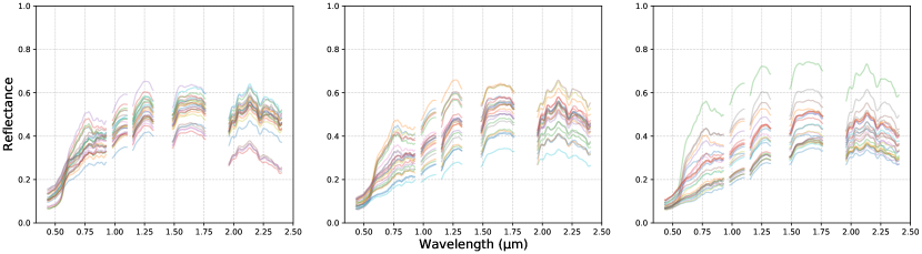
(a) Tile

(b) Asphalt

(c) Vegetation

(d) Painted sheet metal

Figure 10: Spectra from the (left) labeled, (middle) unlabeled and (right) test real data sets

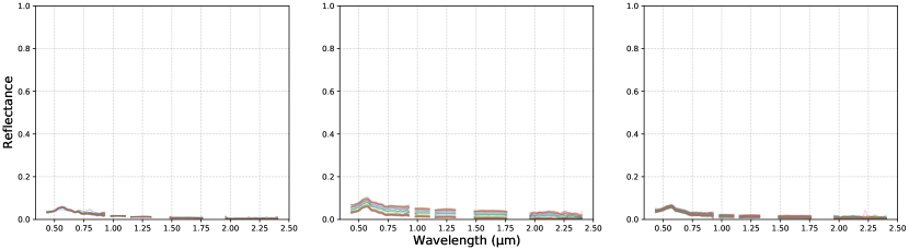
(e) Water

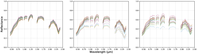
(f) Gravels

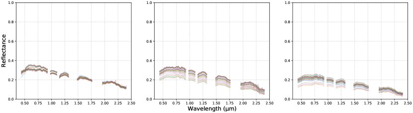
(g) Metal

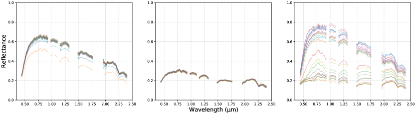
(h) Fiber cement

Figure 10: Spectra from the (left) labeled, (middle) unlabeled and (right) test real data sets

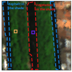
(a)

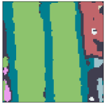
(b)

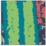
(c)

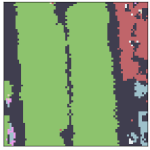
(d)

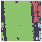
(e)

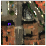
(f)

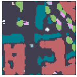
(g)

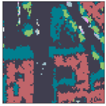
(h)

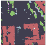
(i)

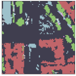
(j)

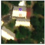
(k)

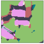
(l)

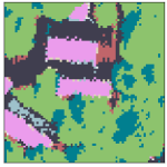
(m)

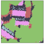
(n)

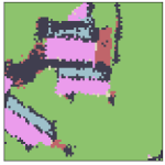
(o)

(p)

Figure 11: (a)-(f)-(k) False color composition of subsets of the AI4GEO hyperspectral image, (b)-(g)-(l) the predictions of FG-UNET, (c)-(h)-(m) the predictions of ssInfoGAN, (d)-(i)-(n) the predictions of the gaussian VAE, (e)-(j)-(o) the predictions of the physics-guided VAE. FG-UNET predictions are spatially consistent but confuses asphalt in the shadows with water, as ssInfoGAN.

References

- [1] Maziar Raissi, Paris Perdikaris, and George E Karniadakis. Physics-informed neural networks: A deep learning framework for solving forward and inverse problems involving nonlinear partial differential equations. Journal of Computational physics, 378:686–707, 2019.
- [2] Naoya Takeishi and Alexandros Kalousis. Physics-integrated variational autoencoders for robust and interpretable generative modeling. Advances in Neural Information Processing Systems, 34:14809–14821, 2021.
- [3] Tom M Mitchell. The need for biases in learning generalizations. Department of Computer Science, Laboratory for Computer Science Research …, 1980.
- [4] Shengjia Zhao, Hongyu Ren, Arianna Yuan, Jiaming Song, Noah Goodman, and Stefano Ermon. Bias and generalization in deep generative models: An empirical study. Advances in Neural Information Processing Systems, 31, 2018.
- [5] Christian Jacobsen and Karthik Duraisamy. Disentangling generative factors of physical fields using variational autoencoders. arXiv preprint arXiv:2109.07399, 2021.
- [6] C Wei, J Zhang, and Chenglin Wu. Thermodynamic consistent neural networks for learning material interfacial mechanics. In NeurIP workshop, 2020.
- [7] Nathaniel Trask, Carianne Martinez, Kookjin Lee, and Brad Boyce. Unsupervised physics-informed disentanglement of multimodal data for high-throughput scientific discovery. arXiv preprint arXiv:2202.03242, 2022.
- [8] Diederik P Kingma and Max Welling. Auto-encoding variational bayes. stat, 1050:1, 2014.
- [9] Irina Higgins, Loic Matthey, Xavier Glorot, Arka Pal, Benigno Uria, Charles Blundell, Shakir Mohamed, and Alexander Lerchner. Early visual concept learning with unsupervised deep learning. stat, 1050:20, 2016.
- [10] Irina Higgins, Loic Matthey, Arka Pal, Christopher Burgess, Xavier Glorot, Matthew Botvinick, Shakir Mohamed, and Alexander Lerchner. beta-vae: Learning basic visual concepts with a constrained variational framework. 2016.
- [11] Mikhail Figurnov, Shakir Mohamed, and Andriy Mnih. Implicit reparameterization gradients. Advances in neural information processing systems, 31, 2018.
- [12] Weonyoung Joo, Wonsung Lee, Sungrae Park, and Il-Chul Moon. Dirichlet variational autoencoder. Pattern Recognition, 107:107514, 2020.
- [13] Yijun Xiao, Tiancheng Zhao, and William Yang Wang. Dirichlet variational autoencoder for text modeling. arXiv preprint arXiv:1811.00135, 2018.
- [14] Emilien Dupont. Learning disentangled joint continuous and discrete representations. Advances in Neural Information Processing Systems, 31, 2018.
- [15] Miguel A Aragon-Calvo and JC Carvajal. Self-supervised learning with physics-aware neural networks–i. galaxy model fitting. Monthly Notices of the Royal Astronomical Society, 498(3):3713–3719, 2020.
- [16] Durk P Kingma, Shakir Mohamed, Danilo Jimenez Rezende, and Max Welling. Semi-supervised learning with deep generative models. Advances in neural information processing systems, 27, 2014.
- [17] Chacha Chen, Guanjie Zheng, Hua Wei, and Zhenhui Li. Physics-informed generative adversarial networks for sequence generation with limited data. In NeurIPS Workshop on Interpretable Inductive Biases and Physically Structured Learning, 2020.
- [18] Sifan Wang, Yujun Teng, and Paris Perdikaris. Understanding and mitigating gradient flow pathologies in physics-informed neural networks. SIAM Journal on Scientific Computing, 43(5):A3055–A3081, 2021.
- [19] Cagatay Yildiz, Markus Heinonen, and Harri Lahdesmaki. Ode2vae: Deep generative second order odes with bayesian neural networks. Advances in Neural Information Processing Systems, 32, 2019.
- [20] Ori Linial, Neta Ravid, Danny Eytan, and Uri Shalit. Generative ode modeling with known unknowns. In Proceedings of the Conference on Health, Inference, and Learning, pages 79–94, 2021.
- [21] Tejas D Kulkarni, William F Whitney, Pushmeet Kohli, and Josh Tenenbaum. Deep convolutional inverse graphics network. Advances in neural information processing systems, 28, 2015.
- [22] Zheng Ding, Yifan Xu, Weijian Xu, Gaurav Parmar, Yang Yang, Max Welling, and Zhuowen Tu. Guided variational autoencoder for disentanglement learning. In Proceedings of the IEEE/CVF Conference on Computer Vision and Pattern Recognition, pages 7920–7929, 2020.
- [23] Elliott Gordon Rodriguez. On disentanglement and mutual information in semi-supervised variational auto-encoders. In Proceedings of the IEEE/CVF Conference on Computer Vision and Pattern Recognition, pages 1257–1262, 2021.
- [24] Ricky TQ Chen, Xuechen Li, Roger B Grosse, and David K Duvenaud. Isolating sources of disentanglement in variational autoencoders. Advances in neural information processing systems, 31, 2018.
- [25] Yann LeCun and Corinna Cortes. MNIST handwritten digit database. 2010.
- [26] Jesper E Van Engelen and Holger H Hoos. A survey on semi-supervised learning. Machine Learning, 109(2):373–440, 2020.
- [27] Isaac Triguero, Salvador García, and Francisco Herrera. Self-labeled techniques for semi-supervised learning: taxonomy, software and empirical study. Knowledge and Information systems, 42(2):245–284, 2015.
- [28] Rifai Salah, P Vincent, X Muller, et al. Contractive auto-encoders: Explicit invariance during feature extraction. In Proc. of the 28th International Conference on Machine Learning, pages 833–840, 2011.
- [29] Dumitru Erhan, Aaron Courville, Yoshua Bengio, and Pascal Vincent. Why does unsupervised pre-training help deep learning? In Proceedings of the thirteenth international conference on artificial intelligence and statistics, pages 201–208. JMLR Workshop and Conference Proceedings, 2010.
- [30] Marc’Aurelio Ranzato and Martin Szummer. Semi-supervised learning of compact document representations with deep networks. In Proceedings of the 25th international conference on Machine learning, pages 792–799, 2008.
- [31] Jason Weston, Frédéric Ratle, Hossein Mobahi, and Ronan Collobert. Deep learning via semi-supervised embedding. In Neural networks: Tricks of the trade, pages 639–655. Springer, 2012.
- [32] Salah Rifai, Grégoire Mesnil, Pascal Vincent, Xavier Muller, Yoshua Bengio, Yann Dauphin, and Xavier Glorot. Higher order contractive auto-encoder. In Joint European conference on machine learning and knowledge discovery in databases, pages 645–660. Springer, 2011.
- [33] Takeru Miyato, Shin-ichi Maeda, Masanori Koyama, and Shin Ishii. Virtual adversarial training: a regularization method for supervised and semi-supervised learning. IEEE transactions on pattern analysis and machine intelligence, 41(8):1979–1993, 2018.
- [34] Javiera Castillo-Navarro, Bertrand Le Saux, Alexandre Boulch, Nicolas Audebert, and Sébastien Lefèvre. Semi-supervised semantic segmentation in earth observation: The minifrance suite, dataset analysis and multi-task network study. Machine Learning, pages 1–36, 2021.
- [35] Ian Goodfellow, Jean Pouget-Abadie, Mehdi Mirza, Bing Xu, David Warde-Farley, Sherjil Ozair, Aaron Courville, and Yoshua Bengio. Generative adversarial nets. Advances in neural information processing systems, 27, 2014.
- [36] Danilo Rezende and Shakir Mohamed. Variational inference with normalizing flows. In International conference on machine learning, pages 1530–1538. PMLR, 2015.
- [37] Adrian Spurr, Emre Aksan, and Otmar Hilliges. Guiding infogan with semi-supervision. In Joint European Conference on Machine Learning and Knowledge Discovery in Databases, pages 119–134. Springer, 2017.
- [38] Xi Chen, Yan Duan, Rein Houthooft, John Schulman, Ilya Sutskever, and Pieter Abbeel. Infogan: Interpretable representation learning by information maximizing generative adversarial nets. Advances in neural information processing systems, 29, 2016.
- [39] Pavel Izmailov, Polina Kirichenko, Marc Finzi, and Andrew Gordon Wilson. Semi-supervised learning with normalizing flows. In International Conference on Machine Learning, pages 4615–4630. PMLR, 2020.
- [40] Danilo Jimenez Rezende, Shakir Mohamed, and Daan Wierstra. Stochastic backpropagation and approximate inference in deep generative models. In International conference on machine learning, pages 1278–1286. PMLR, 2014.
- [41] C. Miesch, L. Poutier, V. Achard, X. Briottet, X. Lenot, and Y. Boucher. Direct and inverse radiative transfer solutions for visible and near-infrared hyperspectral imagery. IEEE Transactions on Geoscience and Remote Sensing, 43(7):1552–1562, 2005.
- [42] Guillaume Roussel, Christiane Weber, Xavier Briottet, and Xavier Ceamanos. Comparison of two atmospheric correction methods for the classification of spaceborne urban hyperspectral data depending on the spatial resolution. International Journal of Remote Sensing, 39(5):1593–1614, December 2017.
- [43] Jean-Philippe Gastellu-Etchegorry, Eloi Grau, and Nicolas Lauret. Dart: A 3d model for remote sensing images and radiative budget of earth surfaces. Modeling and simulation in engineering, (2), 2012.
- [44] L. Roupioz, X. Briottet, K. Adeline, A. Al Bitar, D. Barbon-Dubosc, R. Barda-Chatain, P. Barillot, S. Bridier, E. Carroll, C. Cassante, A. Cerbelaud, P. Déliot, P. Doublet, P.E. Dupouy, S. Gadal, S. Guernouti, A. De Guilhem De Lataillade, A. Lemonsu, R. Llorens, R. Luhahe, A. Michel, A. Moussous, M. Musy, F. Nerry, L. Poutier, A. Rodler, N. Riviere, T. Riviere, J.L. Roujean, A. Roy, A. Schilling, D. Skokovic, and J. Sobrino. Multi-source datasets acquired over toulouse (france) in 2021 for urban microclimate studies during the camcatt/ai4geo field campaign. Data in Brief, 48:109109, 2023.
- [45] Nicolas Audebert, Bertrand Le Saux, and Sébastien Lefèvre. Deep learning for classification of hyperspectral data: A comparative review. IEEE geoscience and remote sensing magazine, 7(2):159–173, 2019.
- [46] Andrei Stoian, Vincent Poulain, Jordi Inglada, Victor Poughon, and Dawa Derksen. Land cover maps production with high resolution satellite image time series and convolutional neural networks: Adaptations and limits for operational systems. Remote Sensing, 11(17):1986, 2019.
- [47] Olaf Ronneberger, Philipp Fischer, and Thomas Brox. U-net: Convolutional networks for biomedical image segmentation. pages 234–241, 2015.
- [48] Yarin Gal and Zoubin Ghahramani. Dropout as a bayesian approximation: Representing model uncertainty in deep learning. In Maria Florina Balcan and Kilian Q. Weinberger, editors, Proceedings of The 33rd International Conference on Machine Learning, volume 48 of Proceedings of Machine Learning Research, pages 1050–1059, New York, New York, USA, 20–22 Jun 2016. PMLR.
- [49] Diederik P Kingma and Jimmy Ba. Adam: A method for stochastic optimization. arXiv preprint arXiv:1412.6980, 2014.
- [50] Martin Arjovsky, Soumith Chintala, and Léon Bottou. Wasserstein generative adversarial networks. pages 214–223, 2017.
- [51] Ishaan Gulrajani, Faruk Ahmed, Martin Arjovsky, Vincent Dumoulin, and Aaron C Courville. Improved training of wasserstein gans. Advances in neural information processing systems, 30, 2017.
- [52] Kien Do and Truyen Tran. Theory and evaluation metrics for learning disentangled representations, 2019.
- [53] Julian Zaidi, Jonathan Boilard, Ghyslain Gagnon, and Marc-André Carbonneau. Measuring disentanglement: A review of metrics. CoRR, abs/2012.09276, 2020.
- [54] Ricky T. Q. Chen, Xuechen Li, Roger B Grosse, and David K Duvenaud. Isolating sources of disentanglement in variational autoencoders. In S. Bengio, H. Wallach, H. Larochelle, K. Grauman, N. Cesa-Bianchi, and R. Garnett, editors, Advances in Neural Information Processing Systems, volume 31. Curran Associates, Inc., 2018.