hp-robust multigrid solver on locally refined meshes
for FEM discretizations of symmetric elliptic PDEs

Abstract.

In this work, we formulate and analyze a geometric multigrid method for the iterative solution of the discrete systems arising from the finite element discretization of symmetric second-order linear elliptic diffusion problems. We show that the iterative solver contracts the algebraic error robustly with respect to the polynomial degree $p\geq 1$ and the (local) mesh size $h$. We further prove that the built-in algebraic error estimator which comes with the solver is $hp$-robustly equivalent to the algebraic error. The application of the solver within the framework of adaptive finite element methods with quasi-optimal computational cost is outlined. Numerical experiments confirm the theoretical findings.

Key words: adaptive finite element method, local multigrid, $hp$-robustness, stable decomposition

AMS subject classifications: 65N12, 65N30, 65N55, 65Y20

1. Introduction

Numerical schemes for PDEs aim at approximating the solution $u^{\star}$ of the weak formulation with an error below a certain tolerance at minimal computational cost. Since the accuracy is spoiled by singularities, e.g., in given data or domain geometry, adaptive finite element methods (AFEMs) employ the loop

to obtain a sequence of meshes $\mathcal{T}_{L}$ that resolve such singularities. For a large class of problems, it is known that AFEM is rate-optimal, i.e., one can construct an estimator $\eta_{L}(u_{L}^{\star})$ from the exact Galerkin solution $u_{L}^{\star}$ for the discretization error $|\!|\!|u^{\star}-u_{L}^{\star}|\!|\!|$ that decreases with the largest possible rate with respect to the number elements in $\mathcal{T}_{L}$; see, e.g., the seminal works [Dör96, MNS00, BDD04, Ste07, CKNS08] or the abstract overview [CFPP14] for $h$-adaptive FEM with fixed polynomial degree $p$.

In practice, the SOLVE module may become computationally expensive (in contrast to all other modules) when employing a direct solver; see, e.g., [PP20, GHPS21, IP23] for a discussion of implementational aspects. Thus, usually, an iterative solver is employed to compute an approximation $u_{L}$ of $u_{L}^{\star}$ on each level, and the exact Galerkin solution $u_{L}^{\star}$ is not available. The question of whether the approximations $u_{L}$ converge with optimal rate with respect to the overall computational cost was already treated in the seminal work [Ste07] under some realistic assumptions about an abstract iterative solver. The recent work [GHPS21] employs nested iterations and an adaptive stopping criterion to steer a uniformly contractive iterative solver, linking the SOLVE and ESTIMATE module in the above scheme by an inner loop. Then, it is shown that even the full sequence of iterates converges with optimal rates with respect to the overall computational cost. For this reason, the design of algebraic solvers that are uniformly contractive and robust with respect to the discretization parameters is of utmost importance.

The hierarchical structure of AFEM and the very nature of the arising linear systems suggest to use a multilevel solver; see, e.g., [Hac85, BMR85, BPS86, BDY88, BPX90, Zha92, Rüd93a, Osw94]. Different adaptive methods integrating a multilevel solver are possible; see, e.g., [BB87] for generating local meshes, and [Rüd93] for a fully adaptive multigrid method that steers the local refinement process. In the context of AFEM, the adaptively constructed hierarchy of locally refined meshes calls for suitable local solvers. We refer to [CNX12] for a multilevel preconditioner on a mesh hierarchy consisting of one bisection in each step and [HWZ12, WZ17] for multiplicative multigrid methods, all of which are robust with respect to the mesh size $h$. Though these works allow for higher-order FEM, an analytic and numerical study on the behavior with increasing polynomial degree was not presented. This aspect is treated, e.g., in [Pav94, SMPZ08, AMV18, BF22], which design iterative solvers that are robust with respect to the polynomial degree $p$ on various types of polyhedral meshes. The recent own work [MPV21] proposes a $p$-robust geometric multigrid which comes with a built-in algebraic error estimator $\zeta_{L}(u_{L})$, which is suited perfectly for a posterori steering (i.e., adaptive termination) of the algebraic solver. However, the employed patchwise smoothing associated to every vertex and every level causes a linear dependence on the number of adaptive mesh levels $L$.

In the present work, we modify the solver from [MPV21] and overcome this dependence for locally refined meshes: we only apply local lowest-order smoothing on patches which change in the refinement step on intermediate levels, whereas a patchwise (and hence parallelizable) higher-order smoothing on all patches of the finest level is applied. This solver only needs one post-smoothing step, requires no symmetrization of the procedure (see also [DHM+21]), and, in particular, has no tunable parameters since it utilizes optimal step-sizes on the error-correction stage. As the main result of the present work, we show that the proposed solver uniformly contracts the algebraic error $|\!|\!|u_{L}^{\star}-u_{L}|\!|\!|$. Moreover, it comes with a built-in estimator $\zeta_{L}(u_{L})$, which is shown to be equivalent to $|\!|\!|u_{L}^{\star}-u_{L}|\!|\!|$. Throughout, all involved estimates are robust in the discretization parameters $h$ and $p$.

As one potential application, we formulate an AFEM algorithm in the spirit of [GHPS21] that naturally embeds the multigrid solver and leverages the solver’s built-in algebraic error estimator $\zeta_{L}(u_{L})$ to stop the solver as soon as the discretization and algebraic error are comparable. Adapting the arguments of [GHPS21], we prove that, for fixed polynomial degree $p$, the AFEM algorithm guarantees optimal convergence rates with respect to overall computational cost.

Using the open-source object-oriented 2D Matlab code MooAFEM [IP23], we present a detailed numerical study of both the algebraic solver and the adaptive algorithm, including higher-order experiments and jumping coefficients.

The outline of this paper reads as follows: Section 2 first poses the model problem and introduces some notation. Then, we state the proposed multigrid solver (Algorithm 2.3) and formulate our main results on $hp$-robust contraction (Theorem 2.4) and algebraic error control (Corollary 2.5). As a potential application, Section 3 formulates an AFEM algorithm (Algorithm 3) which employs nested iteration and an adaptive stopping criterion for the iterative solver using the built-in a posteriori estimator for the algebraic error. Theorem 3.1 proves optimal computational complexity of the proposed AFEM algorithm. After we confirm the theoretical results by numerical examples in Section 4, we present proofs of the main results in Section 5. For better readability, we precede these proofs with three subsections presenting their core arguments: geometric properties of the meshes $\mathcal{T}_{L}$, an $hp$-robust stable decomposition combining a local lowest-order multilevel stable decomposition from [WZ17] with a one-level $p$-robust decomposition from [SMPZ08], and a strengthened Cauchy–Schwarz inequality in the spirit of [CNX12, HWZ12].

2. hp-robust multigrid solver

In this section, we formulate the model problem, the proposed geometric multigrid method, and the main results, while the proofs are postponed to Section 5.

2.1. Model problem

For ${d\!\in\!\{1,2,3\}}$, let ${\Omega\!\subset\!\mathbb{R}^{d}}$ be a bounded Lipschitz domain with polygonal boundary $\partial\Omega$. Given $f\in L^{2}(\Omega)$ and $\bm{f}\in[L^{2}(\Omega)]^{d}$, we consider the second-order linear elliptic diffusion problem

$$\begin{split}-{\rm div}(\bm{K}\nabla u^{\star})&=f-{\rm div}\bm{f}\phantom{0}\text{in }\Omega,\\ u^{\star}&=0\phantom{f-{\rm div}\bm{f}}\text{on }\partial\Omega,\end{split}$$ (1)

where $\bm{K}\in[L^{\infty}(\Omega)]^{d\times d}_{\mathrm{sym}}$ is the symmetric and uniformly positive definite diffusion coefficient. More precisely, given a conforming simplicial triangulation $\mathcal{T}_{h}$ of $\Omega$ into compact simplices, we have $\bm{K}|_{T}\in[W^{1,\infty}(T)]^{d\times d}$ for all $T\in\mathcal{T}_{h}$. For $x\in\Omega$ we denote the maximal and minimal eigenvalue of $\bm{K}(x)\in\mathbb{R}^{d\times d}_{\rm sym}$ by $\lambda_{\max}(\bm{K}(x))$ and $\lambda_{\min}(\bm{K}(x))$, respectively, and define $\Lambda_{\max}\coloneqq\operatorname*{ess\,sup}_{x\in\Omega}\lambda_{\max}(\bm{K}(x))$ as well as $\Lambda_{\min}\coloneqq\operatorname*{ess\,inf}_{x\in\Omega}\lambda_{\min}(\bm{K}(x))$. With $\langle\cdot\,,\,\cdot\rangle_{\omega}$ denoting the usual $L^{2}(\omega)$-scalar product for a measurable subset $\omega\subseteq\Omega$, the weak formulation of (1) seeks $u^{\star}\in\mathbb{V}:=H^{1}_{0}(\Omega)$ solving

$$\lAngle u^{\star}\,,\,v\rAngle_{\Omega}:=\langle\bm{K}\nabla u^{\star}\,,\,\nabla v\rangle_{\Omega}=\langle f\,,\,v\rangle_{\Omega}+\langle\bm{f}\,,\,\nabla v\rangle_{\Omega}\eqqcolon F(v)\quad\text{for all }v\in\mathbb{V}.$$ (2)

We note that $\lAngle\cdot\,,\,\cdot\rAngle_{\Omega}$ is a scalar product and the induced semi-norm $|\!|\!|u|\!|\!|_{\Omega}^{2}:=\lAngle u\,,\,u\rAngle_{\Omega}$ is an equivalent norm on $\mathbb{V}$. Therefore, the Lax–Milgram lemma yields existence and uniqueness of the weak solution $u^{\star}\in\mathbb{V}$. For $\omega=\Omega$, we omit the index $\omega$ throughout.

To discretize (2), denote for a polynomial degree $p\geq 1$ and a triangle $T\in\mathcal{T}_{h}$ the space of all polynomials on $T$ of degree at most $p$ with $\mathbb{P}^{p}(T)$ and define

$$\mathbb{S}^{q}(\mathcal{T}_{h})\!:=\big{\{}v_{h}\in C(\Omega)\,:\,v_{h}|_{T}\in\mathbb{P}^{q}(T)\ \text{for all }T\!\in\!\mathcal{T}_{h}\big{\}}\quad\text{with }q\in\{1,p\}.$$ (3)

With the definition $\mathbb{V}_{h}^{p}\coloneqq\mathbb{S}^{p}_{0}(\mathcal{T}_{h})\coloneqq\mathbb{S}^{p}(\mathcal{T}_{h})\cap H^{1}_{0}(\Omega)$, the discrete problem consists of finding $u^{\star}_{h}\in\mathbb{V}^{p}_{h}$ such that

$$\lAngle u^{\star}_{h}\,,\,v_{h}\rAngle =F(v_{h})\quad\text{for all }v_{h}\in\mathbb{V}_{h}^{p}.$$ (4)

Clearly, the formulation of the discrete problem (4) hinges on the choice of the mesh $\mathcal{T}_{h}$, which directly influences the quality of $u^{\star}_{h}$ as an approximation of $u^{\star}$. Note that (4) can be rewritten as a symmetric and positive definite linear system by introducing a basis of $\mathbb{V}_{h}^{p}$. However, we opt to work instead with the functional basis-independent description.

2.2. Mesh and space hierarchy

We suppose that the refinement strategy in the module REFINE is newest vertex bisection (NVB); see, e.g., [Tra97, Ste08] and Figure 1 for an illustration in $2\mathrm{D}$.

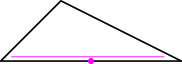
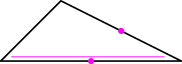
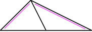
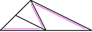
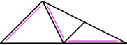
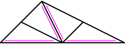
Figure 1. Schematic of 2D NVB refinement pattern: For each triangle $T\in\mathcal{T}$, there is one fixed refinement edge $E_{T}$ indicated by the extra pink line. The pink dots indicate edges that are marked for refinement. If an element is marked for refinement, at least its refinement edge is marked for refinement (top). Iterated bisection refines a marked element into 2, 3, or 4 children (bottom).

Let $\mathcal{T}_{0}$ be the conforming initial mesh. We refer to [Ste08] for NVB with admissible $\mathcal{T}_{0}$ and $d\geq 2$, to [KPP13] for NVB with general $\mathcal{T}_{0}$ for $d=2$, and to the recent work [DGS23] for NVB with general $\mathcal{T}_{0}$ in any dimension. Throughout, we suppose that $\mathcal{T}_{0}$ is admissible. In the $1\mathrm{D}$ case, [AFF+13] splits each element into two children of half-length and additionally ensures that any two neighboring elements have uniformly comparable diameter. Let $\mathbb{T}\coloneqq\mathbb{T}(\mathcal{T}_{0})$ be the set of all refinements of $\mathcal{T}_{0}$ that can be obtained by arbitrarily many steps of NVB.

From now on, suppose that we are given a sequence $\{\mathcal{T}_{\ell}\}_{\ell=0}^{L}\subset\mathbb{T}$ of successively refined triangulations, i.e., for all $\ell=1,\dots,L$, it holds that $\mathcal{T}_{\ell}={\tt REFINE}(\mathcal{T}_{\ell-1},\mathcal{M}_{\ell-1})$ is the coarsest conforming triangulation obtained by NVB, where all marked elements $\mathcal{M}_{\ell-1}\subseteq\mathcal{T}_{\ell-1}$ have been refined by (at least) one bisection. We note that NVB-refinement generates meshes that are uniformly $\gamma$-shape regular, i.e.,

$$\max_{\ell=0,\dots,L}\max\limits_{T\in\mathcal{T}_{\ell}}\frac{\operatorname{\mathrm{diam}}(T)}{|T|^{1/d}}\leq\gamma<\infty,$$ (5a)

and

$$\max_{\ell=0,\dots,L}\max_{T\in\mathcal{T}_{\ell}}\max_{\begin{subarray}{c}T^{\prime}\in\mathcal{T}_{\ell}\\ T\cap T^{\prime}\neq\emptyset\end{subarray}}\frac{\operatorname{\mathrm{diam}}(T)}{\operatorname{\mathrm{diam}}(T^{\prime})}\leq\gamma<\infty.$$ (5b)

where $\gamma$ depends only on $\mathcal{T}_{0}$ and is, in particular, independent of $L$ and the meshes $\mathcal{T}_{1},\dots,\mathcal{T}_{L}$; see, e.g., [Ste08, Theorem 2.1] for $d\geq 2$ or [AFF+13] for $d=1$. We note that (5a) implies (5b) for $d\geq 2$, while (5a) is trivial with $\gamma=1$ and independent of (5b) for $d=1$. In addition, we define the quasi-uniformity constant

$$C_{\rm qu}:=\min\big{\{}\operatorname{\mathrm{diam}}(T)/\operatorname{\mathrm{diam}}(T^{\prime})\,:\,T,T^{\prime}\in\mathcal{T}_{0}\big{\}}\in(0,1].$$ (6)

For each mesh $\mathcal{T}_{\ell}$, let $\mathcal{V}_{\ell}$ denote the set of vertices. Given a vertex $z\in\mathcal{V}_{\ell}$, we denote by $\mathcal{T}_{\ell,z}:=\big{\{}T\in\mathcal{T}_{\ell}\,:\,z\in T\big{\}}$ the patch of elements of $\mathcal{T}_{\ell}$ that share the vertex $z$. The corresponding (open) patch subdomain is denoted by $\omega_{\ell,z}:={\rm interior}(\bigcup_{T\in\mathcal{T}_{\ell,z}}T)$ and its size by $h_{\ell,z}\coloneqq\max_{T\in\mathcal{T}_{\ell,z}}h_{T}\coloneqq\max_{T\in\mathcal{T}_{\ell,z}}|T|^{1/d}$. Finally, we denote by $\mathcal{V}_{\ell}^{+}$ the set of new vertices in $\mathcal{T}_{\ell}$ and the pre-existing vertices of $\mathcal{T}_{\ell-1}$ whose associated patches have shrunk in size in the refinement step $\ell$, i.e.,

$$\mathcal{V}_{0}^{+}:=\mathcal{V}_{0}\quad\text{and}\quad\mathcal{V}_{\ell}^{+}:=\mathcal{V}_{\ell}\setminus\mathcal{V}_{\ell-1}\cup\big{\{}z\in\mathcal{V}_{\ell}\cap\mathcal{V}_{\ell-1}\,:\,\omega_{\ell,z}\neq\omega_{\ell-1,z}\big{\}}\quad\text{for }\ell\geq 1.$$

While this notation is used in the analysis of the solver below, the presentation of Algorithm 2.3 is more compact with the abbreviation $\mathcal{N}_{\ell}=\mathcal{V}_{\ell}^{+}$ for $\ell=1,\dots,L-1$ and $\mathcal{N}_{L}\coloneqq\mathcal{V}_{L}^{+}$ for $p=1$ and $\mathcal{N}_{L}\coloneqq\mathcal{V}_{L}$ otherwise, where we recall that $p\in\mathbb{N}$ is the fixed polynomial degree of the FEM ansatz functions.

From the definition of the discrete FEM spaces (3) and NVB-refinement, we see that there holds nestedness

$$\mathbb{V}_{0}^{1}\subseteq\mathbb{V}_{1}^{1}\subseteq\dots\subseteq\mathbb{V}_{L-1}^{1}\subseteq\mathbb{V}_{L}^{p}.$$ (7)

Furthermore, we require the local spaces

$$\mathbb{V}^{q}_{\ell,z}:=\mathbb{S}^{q}_{0}(\mathcal{T}_{\ell,z})\quad\text{for all vertices }z\in\mathcal{V}_{\ell}\text{ and }q\in\{1,p\},$$ (8)

where we use $q=1$ for $\ell=0,\dots,L-1$ and $q=p$ for $\ell=L$; see Figure 2 for the illustration of the degrees of freedom for $p=2$.

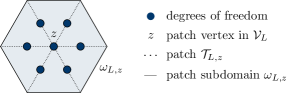
Figure 2. Illustration of degrees of freedom ($p=2$) for the space $\mathbb{V}_{L,z}^{p}$ associated to the patch $\mathcal{T}_{L,z}$.

2.3. Multigrid solver

In the following, we introduce a local geometric multigrid method, which will serve as iterative solver within the SOLVE module of an adaptive FEM algorithm. Each full step of the proposed multigrid method can be mathematically described by an iteration operator $\Phi\colon\mathbb{V}_{L}^{p}\to\mathbb{V}_{L}^{p}$, i.e., given the current approximation $u_{L}\in\mathbb{V}_{L}^{p}$, the solver generates the new iterate $\Phi(u_{L})\in\mathbb{V}_{L}^{p}$.

The main ingredients in the solver construction are an inexpensive global residual solve on $\mathcal{T}_{0}$ and local residual solves on all patches $\mathcal{T}_{\ell,z}$ for $z\in\mathcal{V}_{\ell}^{+}$ on the intermediate levels $\ell=1,\ldots,L-1$ and all patches on the finest level $\mathcal{T}_{L}$ when $p>1$. For ease of notation, we define the algebraic residual functional $R_{L}\colon\mathbb{V}_{L}^{p}\to\mathbb{R}$ by

$$v_{L}\in\mathbb{V}_{L}^{p}\mapsto R_{L}(v_{L}):=F(v_{L})-\lAngle u_{L}\,,\,v_{L}\rAngle=\lAngle u_{L}^{\star}-u_{L}\,,\,v_{L}\rAngle\in\mathbb{R}.$$ (9)

To construct the new iterate $\Phi(u_{L})$, levelwise residual liftings of the algebraic error are added to the current approximation $u_{L}$. The same levelwise residual liftings are used to define an a posteriori error estimator $\zeta_{L}(u_{L})$ for the algebraic error, i.e., the solver comes with a built-in estimator.

[One step of the optimal local multigrid solver] Input: Current approximation $u_{L}\in\mathbb{V}_{L}^{p}$, meshes $\{\mathcal{T}_{\ell}\}_{\ell=0}^{L}$, polynomial degree $p\in\mathbb{N}$.
Solver step: Perform the following steps (i)–(ii):

1. Global lowest-order residual problem on the coarsest level:

   • Compute $\rho_{0}\in\mathbb{V}_{0}^{1}$ by solving

     $$\lAngle\rho_{0}\,,\,v_{0}\rAngle=R_{L}(v_{0})\quad\text{for all }v_{0}\in\mathbb{V}_{0}^{1}.$$ (10)

   • Define step-size $\lambda_{0}:=1$.

   • Initialize algebraic lifting $\sigma_{0}:=\lambda_{0}\rho_{0}$ and a posteriori estimator ${\zeta_{0}^{2}\!:=\!|\!|\!|\lambda_{0}\rho_{0}|\!|\!|^{2}}\!$.

2. Local residual-update: For all $\ell=1,\dots,L$, do the following steps, where $q=1$ for $\ell=1,\dots,L-1$ and $q=p$ for $\ell=L$:

   • For all $z\in\mathcal{N}_{\ell}$, compute $\rho_{\ell,z}\in\mathbb{V}_{\ell,z}^{q}$ by solving

     $$\lAngle\rho_{\ell,z}\,,\,v_{\ell,z}\rAngle=R_{L}(v_{\ell,z})-\lAngle\sigma_{\ell-1}\,,\,v_{\ell,z}\rAngle\quad\text{for all }v_{\ell,z}\in\mathbb{V}_{\ell,z}^{q}.$$ (11)

   • Define the line-search step-size $s_{\ell}:=(R_{L}(\rho_{\ell})-\lAngle\sigma_{\ell-1}\,,\,\rho_{\ell}\rAngle)/|\!|\!|\rho_{\ell}|\!|\!|^{2}$, with $\rho_{\ell}:=\sum_{z\in\mathcal{N}_{\ell}}\rho_{\ell,z}$ and the understanding that $0/0\coloneqq 0$ if $\rho_{\ell}=0$, and

     $$\lambda_{\ell}\!\coloneqq\begin{cases}s_{\ell}&\text{if }s_{\ell}\leq d+1\ \text{ or $\big{[}\ell=L$ and $p>1\big{]}$},\\ (d+1)^{-1}&\,\textrm{otherwise.}\end{cases}$$

   • Update $\sigma_{\ell}:=\sigma_{\ell-1}+\lambda_{\ell}\rho_{\ell}$ and $\zeta_{\ell}^{2}:=\zeta_{\ell-1}^{2}+\lambda_{\ell}\sum_{z\in\mathcal{N}_{\ell}}|\!|\!|\rho_{\ell,z}|\!|\!|^{2}$.

Output: Improved approximation $\Phi(u_{L}):=u_{L}+\sigma_{L}\in\mathbb{V}_{L}^{p}$ and associated a posteriori estimator $\zeta_{L}(u_{L}):=\zeta_{L}$ of the algebraic error.

Remark 2.1 (Construction of the new iterate).

The construction of $\Phi(u_{L})$ from $u_{L}$ by Algorithm 2.3 can be seen as one iteration of a V-cycle multigrid with no pre- and one post-smoothing step, and a step-size at the error correction stage. The smoother on each level is additive Schwarz associated to patch subdomains where the local problems (11) are defined. This is equivalent to diagonal Jacobi smoothing for $p=1$ (e.g., on intermediate levels) and block-Jacobi smoothing for $p>1$ (e.g., on the finest level). The choice and use of the step-sizes $\lambda_{\ell}$ in Algorithm 2.3 (ii) comes from a line-search approach; see, e.g., [MPV21, Lemma 4.3] and one of the earlier works [Hei88]. However, if the step-size from the line-search is too large, we use instead a fixed damping parameter offsetting the $d+1$ patch overlaps. We note that this case never occurred in practice in any of our numerical experiments.

Remark 2.2 (Computational effort and speed of convergence).

We note that we apply a patchwise Cholesky factorization on the finest level. Hence, the computational effort for the local residual solve on the finest mesh $\mathcal{T}_{L}$ in dependence on the polynomial degree $p$ is of order $\mathcal{O}(p^{3d}\#\mathcal{T}_{L})$. The presented algorithm is a linear method. One could symmetrize the procedure by adding one pre-smoothing step to define a preconditioner in the hope of accelerating convergence with the help of conjugate gradients. However, in our experience, the patchwise pre-smoothing typically did not yield considerable algebraic error decrease; see, e.g. [DHM+21], while still doubling the number of smoothing operations of a V-cycle. The remaining steps needed to compute the new approximation stem from classical multigrid solvers (such as intergrid operators). We stress that the overall effort does not depend on the number of levels $L$.

Remark 2.3 (Nested iterations).

In the context of adaptive FEM, the solver does not start from an arbitrary initial guess on each newly-refined mesh but from the final approximation of the previous level (see Algorithm 3 below). This will ensure a posteriori error control in each step after initialization as well as optimal computational cost. From the algebraic solver perspective, such an approach can be seen as a full multigrid method over the evolving hierarchy of meshes whose number of cycles is determined by the adaptive stopping criterion.

2.4. Main result

This subsection formulates the main results regarding the iterative solver stating the contraction of the multigrid solver and reliability of the built-in a posteriori estimator of the algebraic error. Both results hold robustly in the number of levels $L$ and the polynomial degree $p$.

Theorem 2.4.

Let $u_{L}^{\star}\in\mathbb{V}_{L}^{p}$ be the (unknown) finite element solution of (4) and let $v_{L}\in\mathbb{V}_{L}^{p}$ be arbitrary. Let $\Phi(v_{L})\in\mathbb{V}_{L}^{p}$ and $\zeta_{L}(v_{L})$ be generated by Algorithm 2.3. Then, the solver iterates and the estimator are connected by

$$|\!|\!|u_{L}^{\star}-\Phi(v_{L})|\!|\!|^{2}\leq|\!|\!|u_{L}^{\star}-v_{L}|\!|\!|^{2}-\zeta_{L}(v_{L})^{2}.$$ (12)

Moreover, the solver contracts the error, i.e., there exists $0<q_{\rm ctr}<1$ such that

$$|\!|\!|u_{L}^{\star}-\Phi(v_{L})|\!|\!|\leq q_{\rm ctr}\,|\!|\!|u_{L}^{\star}-v_{L}|\!|\!|.$$ (13)

Finally, the estimator is a two-sided bound of the algebraic error, i.e., there exists $C_{\rm rel}>1$ such that

$$\zeta_{L}(v_{L})\leq|\!|\!|u_{L}^{\star}-v_{L}|\!|\!|\leq C_{\rm rel}\,\zeta_{L}(v_{L}).$$ (14)

The contraction and reliability constants $q_{\rm ctr}$ and $C_{\rm rel}$ depend only on the space dimension $d$, the $\gamma$-shape regularity (5), the quasi-uniformity constant $C_{\rm qu}$ from (6), $\Lambda_{\max}/\Lambda_{\min}$, and $\max_{T\in\mathcal{T}_{L}}\|\operatorname{\mathrm{div}}(\bm{K})\|_{L^{\infty}(T)}/\Lambda_{\min}$. In particular, $q_{\rm ctr}$ is independent of the polynomial degree $p$, the number of mesh levels $L$, and the meshes $\mathcal{T}_{1},\dots,\mathcal{T}_{L}$.

Corollary 2.5.

The reliability of the estimator in (14) is equivalent to the solver contraction (13). In particular, this also yields that

$$|\!|\!|u_{L}^{\star}-\Phi(v_{L})|\!|\!|\leq q_{\rm ctr}C_{\rm rel}\,\zeta_{L}(v_{L}).$$ (15)

Remark 2.6.

We note that (12) holds with equality whenever the step-size criterion $s_{\ell}\leq d+1$ in Algorithm 2.3(ii) are fulfilled and the construction is thus done by optimal-line search. In such a case, which was always satisfied in all our numerical tests, a Pythagoras identity in the spirit of [MPV21, Theorem 4.7] yielding exact algebraic error decrease is obtained.

3. Application to adaptive FEM with inexact solver

Given a coarse mesh $\mathcal{T}_{0}$, we use an adaptive finite element method (AFEM) to generate locally refined meshes $\{\mathcal{T}_{L}\}_{L\in\mathbb{N}}$ tailored to the behavior of the sought solution. In the spirit of [GHPS21], Algorithm 3 presents such an approach with an adaptively stopped iterative solver, where Step (Ii) exploits the built-in a posteriori estimator of the geometric multigrid solver from Section 2.

While we note that the present Algorithm 3 and the corresponding Theorem 3.1 are restricted to fixed polynomial degree $p$, the inclusion of the proposed $hp$-robust iterative solver into the $hp$-adaptive FEM algorithm of [CNSV17] remains for future research, since the mathematical understanding of $hp$-adaptive FEM is still widely open.

[AFEM with iterative solver]  
Input: Initial mesh $\mathcal{T}_{0}$, polynomial degree $p\in\mathbb{N}$, adaptivity parameters $0<\theta\leq 1$, $C_{\rm mark}\geq 1$, and $\mu>0$, initial guess $u_{0}^{0}:=0$.

Adaptive loop: repeat the following steps (I)–(III) for all $L=0,1,2,\dots$:

1. SOLVE & ESTIMATE: repeat the following steps (i)–(iii) for all $k=1,2,3,\dots$:

   1. Do one step of the algebraic solver to obtain $u_{L}^{k}\in\mathbb{V}_{L}^{p}$ and an associated a posteriori estimator $\zeta_{L}(u_{L}^{k-1})$ for the algebraic error

      $$[u_{L}^{k},\zeta_{L}(u_{L}^{k-1})]\ :=\ {\tt SOLVE}(u_{L}^{k-1},\{\mathcal{T}_{\ell}\}_{\ell=0}^{L},p).$$

   2. Compute a posteriori indicators for the elementwise discretization error

      $$\{\eta_{L}(T,u_{L}^{k})\}_{T\in\mathcal{T}_{L}}:={\tt ESTIMATE}(u_{L}^{k},\mathcal{T}_{L}).$$

   3. If $\zeta_{L}(u_{L}^{k-1})\leq\mu\eta_{L}(u_{L}^{k})$, terminate the $k$-loop, set the index ${\underline{k}}[L]\coloneqq k$ and define $u_{L}:=u_{L}^{{\underline{k}}[L]}$.

2. MARK: Determine a set of marked elements $\mathcal{M}_{L}\subseteq\mathcal{T}_{L}$ of (up to the multiplicative constant $C_{\rm mark}$) minimal cardinality that satisfies

   $$\theta\,\eta_{L}(u_{L})^{2}\leq\sum_{T\in\mathcal{M}_{L}}\eta_{L}(T,u_{L})^{2}.$$

3. REFINE: Generate the new mesh $\mathcal{T}_{L+1}:={\tt REFINE}(\mathcal{M}_{L},\mathcal{T}_{L})$ and define $u_{L+1}^{0}:=u_{L}$.

Output: Sequences of successively refined triangulations $\mathcal{T}_{L}$, discrete approximations $u_{L}$ and corresponding error estimators $(\eta_{L}(u_{L}),\zeta_{L}(u_{L}))$. Mesh-refinement is steered by the discretization error estimator. For all $T\in\mathcal{T}_{h}$, let $\eta_{h}(T;\cdot)\colon\mathbb{V}_{h}^{p}\to\mathbb{R}_{\geq 0}$ be the local contributions of the standard residual error estimator defined by

$$\eta_{h}^{2}(T;v_{h})\coloneqq h_{T}^{2}\|f+\operatorname{\mathrm{div}}(\bm{K}\nabla v_{h}-\bm{f})\|_{T}^{2}+h_{T}\|\lBrack\bm{K}\nabla v_{h}-\bm{f}\rBrack\cdot\bm{n}\|_{\partial T\cap\Omega}^{2},$$ (16)

where $\|\cdot\|_{\omega}$ denote the appropriate $L^{2}(\omega)$-norms. We define

$$\eta_{h}(\mathcal{U}_{h};v_{h}):=\Bigl{(}\sum_{T\in\,\mathcal{U}_{h}}\eta_{h}(T;v_{h})^{2}\Bigr{)}^{1/2}\quad\text{for all }\mathcal{U}_{h}\subseteq\mathcal{T}_{h}\text{ and }v_{h}\in\mathbb{V}_{h}^{p}.$$

To abbreviate notation, let $\eta_{h}(v_{h}):=\eta_{h}(\mathcal{T}_{h};v_{h})$.

One important consequence of Theorem 2.4 is optimal convergence of Algorithm 3 with respect to computational complexity. To formulate this mathematically, we define the ordered set

$$\mathcal{Q}\coloneqq\big{\{}(L,k)\in\mathbb{N}_{0}^{2}\,:\,(L,k)\text{ is used as loop variable in Algorithm~{}\ref{algorithm:afem} and $1\leq k\leq{\underline{k}}[L]$}\big{\}}.$$

On $\mathcal{Q}$, we define the ordering $\leq$ by

$$(L^{\prime},k^{\prime})\leq(L,k)\quad\Longleftrightarrow\quad u_{L^{\prime}}^{k^{\prime}}\text{ is computed earlier than or equal to $u_{L}^{k}$ in Algorithm~{}\ref{algorithm:afem}.}$$

Furthermore, we introduce the total step counter $|\cdot,\cdot|$, defined for all $(L,k)\in\mathcal{Q}$, by

$$|L,k|\coloneqq\#\big{\{}(L^{\prime},k^{\prime})\in\mathcal{Q}\,:\,(L^{\prime},k^{\prime})\leq(L,k)\big{\}}.$$

Before we state the theorem, we introduce the notion of approximation classes. For $\mathcal{T}\in\mathbb{T}$ and $s>0$ define

$$\|u\|_{\mathbb{A}_{s}}:=\sup_{N\in\mathbb{N}_{0}}\Big{(}\big{(}N+1\big{)}^{s}\min_{\mathcal{T}_{\rm opt}\in\mathbb{T}_{N}(\mathcal{T}_{0})}\big{(}|\!|\!|u^{\star}-u^{\star}_{\rm opt}|\!|\!|+\eta_{\rm opt}(u^{\star}_{\rm opt})\big{)}\Big{)},$$ (17)

with Galerkin solution $u_{\rm opt}^{\star}$ and estimator $\eta_{\rm opt}$ on the optimal triangulation $\mathcal{T}_{\rm opt}\in\mathbb{T}_{N}(\mathcal{T}_{0})$, where $\mathbb{T}_{N}(\mathcal{T}_{0})\coloneqq\big{\{}\mathcal{T}_{h}\in\mathbb{T}(\mathcal{T}_{0})\,:\,\#\mathcal{T}_{h}-\#\mathcal{T}_{0}\leq N\big{\}}$. By reliability (A3) of the estimator, see, e.g., [CFPP14], the sum on the right-hand side of (17) is equivalent to $\eta_{\rm opt}(u^{\star}_{\rm opt})$. If $\|u\|_{\mathbb{A}_{s}}<\infty$, then we say that rate $s$ is possible. In [GHPS21], it is shown that in the case of a contractive solver, convergence rates with respect to degrees of freedom are equivalent to convergence rates with respect to computational complexity. We abbreviate with $\operatorname*{cost}(L,k)$ the total costs of Algorithm 3 defined by

$$\operatorname*{cost}(L,k)\coloneqq\sum_{\begin{subarray}{c}(L^{\prime},k^{\prime})\in\mathcal{Q}\\ (L^{\prime},k^{\prime})\leq(L,k)\end{subarray}}\#\mathcal{T}_{L^{\prime}}.$$

Theorem 3.1.

Let $\{\mathcal{T}_{L}\}_{L\in\mathbb{N}_{0}}$ be the sequence generated by Algorithm 3 and define the quasi-error by

$$\Delta_{L}^{k}\coloneqq|\!|\!|u^{\star}-u_{L}^{k}|\!|\!|+\eta_{L}(u_{L}^{k})\quad\text{for all }(L,k)\in\mathcal{Q}.$$

Then, for all parameters $0<\theta\leq 1$ and $\mu>0$, it holds that

$$\sup\limits_{(L,k)\in\mathcal{Q}}(\#\mathcal{T}_{L})^{s}\Delta_{L}^{k}\simeq\sup_{(L,k)\in\mathcal{Q}}\operatorname*{cost}(L,k)^{s}\,\Delta_{L}^{k}\quad\text{ and }\quad\Delta_{L}^{k}\to 0\text{ as }|L,k|\to\infty.$$ (18)

Furthermore, there exist $0<\theta^{\star}\leq 1$, and $\mu^{\star}>0$ such that, for sufficiently small parameters $0<\theta<\theta^{\star}$ and $0<\mu/\theta<\mu^{\star}$, and for all $s>0$, it holds that

$$c_{\mathrm{opt}}\,\|u\|_{{\mathbb{A}_{s}}}\leq\sup_{(L,k)\in\mathcal{Q}}\operatorname*{cost}(L,k)^{s}\,\Delta_{L}^{k}\leq C_{\mathrm{opt}}\,\max\{\|u\|_{{\mathbb{A}_{s}}},\Delta_{0}^{0}\}.$$ (19)

The constants $c_{\mathrm{opt}},C_{\mathrm{opt}}>0$ depend only on the polynomial degree $p$, the initial triangulation $\mathcal{T}_{0}$, $\Lambda_{\max}/\Lambda_{\min}$, $\max_{T\in\mathcal{T}_{L}}\|\operatorname{\mathrm{div}}(\bm{K})\|_{L^{\infty}(T)}/\Lambda_{\min}$, the rate $s$, the ratios $\theta/\theta^{\star}$ and $\mu/(\theta\mu^{\star})$, and the properties of newest vertex bisection. In particular, this proves the equivalence

$$\|u\|_{{\mathbb{A}_{s}}}<\infty\quad\Longleftrightarrow\quad\sup_{(L,k)\in\mathcal{Q}}\operatorname*{cost}(L,k)^{s}\,\Delta_{L}^{k}<\infty,$$ (20)

which proves optimal complexity of Algorithm 3.

Remark 3.2.

We note that in [GHPS21, Theorem 8], the constant $c_{\mathrm{opt}}>0$ additionally depends on the stopping index $\underline{L}$ in the case the algorithm terminates after a finite number of mesh levels $\underline{L}<\infty$ or the estimator satisfies $\eta_{L}(u_{L})=0$. The refined analysis in the recent work [BIM+23] removes this dependence.

Remark 3.3.

We note that it is also possible to use the same stopping criterion for the algebraic solver as in [GHPS21, Algorithm 2]. However, since the multigrid solver from Algorithm 2.3 has a built-in estimator for the algebraic error, we opt for its choice within Algorithm 3 instead.

Proof 3.4 (Proof of Theorem 3.1).

We show that Algorithm 3 satisfies the requirements of [GHPS21, Theorem 4 and Theorem 8]. First note that the standard residual error estimator from (16) satisfies the axioms of adaptivity from [CFPP14] and thus satisfies the assumptions (A1)–(A4) from [GHPS21, Theorem 8]. Furthermore, newest vertex bisection satisfies the assumptions (R1)–(R3) from [GHPS21, Section 2.2]. For the present setting, the conditions (C1) and (C2) from [GHPS21, Section 2.5] coincide and are satisfied.

Tracing the role of the stopping criterion for the case (C1) in the proof of [GHPS21, Theorem 4], one sees that the stopping criterion needs to guarantee that, for all $(L,k)\in\mathcal{Q}$,

$$\begin{split}|\!|\!|u_{L}^{k}-u_{L}^{k-1}|\!|\!|&\leq\lambda_{1}\,\eta_{L}(u_{L}^{k})\qquad\text{if }u_{L}^{k}=u_{L},\\ \eta_{L}(u_{L}^{k})&\leq\lambda_{2}^{-1}\,|\!|\!|u_{L}^{k}-u_{L}^{k-1}|\!|\!|\qquad\text{else,}\end{split}$$ (21)

for some $\lambda_{1},\lambda_{2}>0$. The upper bound in (14) in Theorem 2.4 as well as contraction (13) show that, for all $(L,k)\in\mathcal{Q}$, our stopping criterion in Algorithm 3 Step (Iiii) leads for $u_{L}^{k}=u_{L}$ to

$$|\!|\!|u_{L}^{k}-u_{L}^{k-1}|\!|\!|\stackrel{{\scriptstyle\eqref{equation:contraction}}}{{\leq}}(1+q_{\rm ctr})\,|\!|\!|u_{L}^{\star}-u_{L}^{k-1}|\!|\!|\stackrel{{\scriptstyle\eqref{equation:equivalence}}}{{\leq}}C_{\rm rel}\,(1+q_{\rm ctr})\,\zeta_{L}(u_{L}^{k-1})\leq\mu\,C_{\rm rel}\,(1+q_{\rm ctr})\,\eta_{L}(u_{L}^{k}).$$

For the remaining case, the contraction (13) leads to

$$|\!|\!|u_{L}^{\star}-u_{L}^{k}|\!|\!|\stackrel{{\scriptstyle\eqref{equation:contraction}}}{{\leq}}q_{\rm ctr}\,|\!|\!|u_{L}^{\star}-u_{L}^{k-1}|\!|\!|\leq q_{\rm ctr}\,|\!|\!|u_{L}^{\star}-u_{L}^{k}|\!|\!|+q_{\rm ctr}\,|\!|\!|u_{L}^{k}-u_{L}^{k-1}|\!|\!|.$$

This implies

$$|\!|\!|u_{L}^{\star}-u_{L}^{k}|\!|\!|\leq\frac{q_{\rm ctr}}{1-q_{\rm ctr}}|\!|\!|u_{L}^{k}-u_{L}^{k-1}|\!|\!|.$$ (22)

The not met stopping criterion in Algorithm 3(Iiii), the lower bound in (14), and (22) show

$$\eta_{L}(u_{L}^{k})<\mu^{-1}\,\zeta_{L}(u_{L}^{k-1})\stackrel{{\scriptstyle\eqref{equation:equivalence}}}{{\leq}}\mu^{-1}\,|\!|\!|u_{L}^{\star}-u_{L}^{k-1}|\!|\!| \leq\mu^{-1}\,\bigl{(}|\!|\!|u_{L}^{\star}-u_{L}^{k}|\!|\!|+|\!|\!|u_{L}^{k}-u_{L}^{k-1}|\!|\!|\bigr{)}$$

$$\stackrel{{\scriptstyle\mathclap{\eqref{eq:error_control}}}}{{\leq}}\mu^{-1}\,\bigl{(}1+\frac{q_{\rm ctr}}{1-q_{\rm ctr}}\bigr{)}\,|\!|\!|u_{L}^{k}-u_{L}^{k-1}|\!|\!|$$

$$=\mu^{-1}\,\bigl{(}\frac{1}{1-q_{\rm ctr}}\bigr{)}\,|\!|\!|u_{L}^{k}-u_{L}^{k-1}|\!|\!|.$$

Overall, (21) is satisfied with

$$\lambda_{1}=C_{\mathrm{rel}}\,(1+q_{\rm ctr})\,\mu\quad\text{and}\quad\lambda_{2}=(1-q_{\rm ctr})\,\mu,$$

and [GHPS21, Theorem 4] proves full linear convergence, so that, in particular, (18) is fulfilled (see the proof of [GHPS21, Theorem 8] or [BIM+23, Corollary 4.2]).

The lower bound in (19) follows as in [GHPS21, Theorem 8] or [BIM+23, Theorem 4.3]. For the upper bound in (19), [GHPS21, Theorem 8] requires that

$$0<\lambda_{1}/\theta<\lambda_{\mathrm{opt}}\coloneqq(1-q_{\rm ctr})/(q_{\rm ctr}\,C_{\mathrm{stab}})$$

and

$$0<\theta^{\prime}\coloneqq\frac{\theta+\lambda_{1}/\lambda_{\mathrm{opt}}}{1-\lambda_{1}/\lambda_{\mathrm{opt}}}<\theta_{\mathrm{opt}}\coloneqq(1+C_{\mathrm{stab}}^{2}\,C_{\mathrm{drel}}^{2})^{-1},$$

where $C_{\mathrm{stab}}$ is the stability constant from (A1) and $C_{\mathrm{drel}}$ is the constant from discrete reliability (A4); see, e.g., [GHPS21]. We define

$$\mu^{\star}\coloneqq\frac{\lambda_{\mathrm{opt}}}{C_{\mathrm{rel}}\,(1+q_{\rm ctr})},$$

and $\mu/\theta<\mu^{\star}$ thus implies $\lambda_{1}/\theta=C_{\mathrm{rel}}\,(1+q_{\rm ctr})\,\mu/\theta<\lambda_{\mathrm{opt}}$. Finally, we choose $\theta^{\star}$ such that any $0<\widetilde{\theta}\leq\theta^{\star}$ satisfies $\frac{2\,\widetilde{\theta}}{1-\widetilde{\theta}}<\theta_{\mathrm{opt}}$. Then, $0<\theta<\theta^{\star}$ yields $\theta^{\prime}=\frac{\theta+\lambda_{1}/\lambda_{\mathrm{opt}}}{1-\lambda_{1}/\lambda_{\mathrm{opt}}}<\frac{2\,\theta}{1-\theta}<\theta_{\mathrm{opt}}$ and optimal cost in Theorem 3.1 follows directly from [GHPS21, Theorem 8].

4. Numerical experiments

This section investigates the numerical performance of the proposed multigrid solver of Algorithm 2.3 and the adaptive Algorithm 3. The Matlab implementation of the multigrid solver is embedded into the MooAFEM framework from [IP23]. Throughout, we choose the marking parameter $\theta=0.5$ in the adaptive Algorithm 3 and $\bm{f}=(0,0)^{\top}$. We introduce the following test case:

• L-shaped domain. Let $\Omega=(-1,1)^{2}\setminus\big{(}[0,1]\times[-1,0]\big{)}$ with right-hand side $f=1$ and $\bm{K}=\bm{I}$.

4.1. Contraction and performance of local multigrid solver

We confirm numerically our main results from Theorem 2.4. In order to study the algebraic solver and its built-in estimator with respect to different polynomial degrees, we take $\mu=10^{-5}$ in Algorithm 3, thus oversolving the algebraic problem. Moreover, we stop the adaptive algorithm once the final mesh consists of $10^{6}$ degrees of freedom. Note that thanks to Corollary 2.5 proving the equivalence of the reliability of the algebraic error estimator with the contraction of the algebraic solver, we indeed only need to investigate numerically the existence of the $p$-robust bound on the contraction of the solver. In Figure 3 (left), we present the maximal contraction factors on each level $L$ of the adaptive algorithm from Algorithm 3. We see that the contraction factors are robust in the polynomial degree $p$ with an upper bound of about $0.7$ in all our experiments. In Figure 3 (right), we see that on a fixed number of levels ($L$=10) even for higher-order polynomials their behavior is clustered around similar values. Moreover, from a purely solver-centric perspective, we see that the solver variant which employs higher-order smoothing also on the intermediate levels (and not only on the finest one) as studied in [MPV21] only leads to slight improvements of the contraction constants. Adapting the arguments of [MPV21], this modified construction can be guaranteed to be contractive with $p$-robust, but linearly $L$-dependent contraction bound on the algebraic error. However, this degradation with increasing $L$ is not seen in practice, provided that the patchwise smoothing is done everywhere for level $L=1$ (as new degrees of freedom are added on all patches when the polynomial degree is $p>1$) and local patchwise smoothing is employed in the remaining levels. We present a comparison of the resulting contraction factors of this approach to Algorithm 2.3 for a fixed number of level ($L=10$) in Figure 3(right).

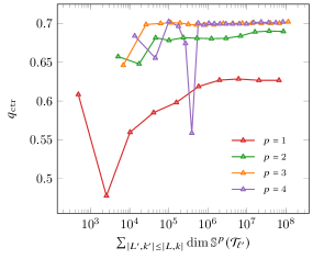
(A)

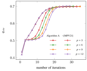
(B)

Figure 3. Contraction of the algebraic solver. History plot of the contraction factors $q_{\rm ctr}$ from (13) for various polynomial degrees $p$ with parameter $\mu=10^{-5}$ for the presented polynomial hierarchy from (7) in the adaptive algorithm from Algorithm 3 stopping once the final mesh consists of $10^{6}$ degrees of freedom (left) and the comparison with polynomial hierarchy motivated by [MPV21] with localized smoothing for a fixed number of levels $L=10$ (right).

4.2. Optimality of the adaptive algorithm

We take $\mu=0.1$ in Algorithm 3 and study the decrease of the discretization error estimator $\eta_{L}(u_{L})$, both in terms of number of degrees of freedom and timing. We remark that the error estimator $\eta_{L}(u_{L})$ on the final iterates is equivalent to the quasi-error $\Delta_{L}$. After a pre-asymptotic phase, we see in Figure 4A and 4B for different polynomial degrees $p$ that the optimal convergence rate $-p/2$ is recovered both with respect to number of degrees of freedom and computational time, and the singularity at the reentrant corner $(0,0)$ is resolved through local mesh refinement. Furthermore, Figure 5 shows that the proposed multigrid solver behaves faster than the built-in direct solver (Matlab backslash operator) concerning the time per dof. The displayed timings include the setup of the linear system, the time for the solver module, computation of estimator, and mesh refinement. Overall, the numerical experiments in Figure 5 validate the linear complexity of the suggested local multigrid solver from Algorithm 2.3.

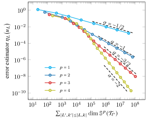
(A)

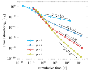
(B)

Figure 4. Optimality of AFEM on L-shape. The convergence history plot of the discretization error estimator $\eta_{L}(u_{L})$ with respect to the total computational cost (left) and the cumulative computational time (right).

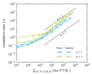
(A)

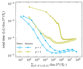
(B)

Figure 5. Optimality of the local multigrid solver. History plot of the cumulative computational time and the relative computational time per degree of freedom for the polynomial degrees $p=1$ and $p=4$. We compare the overall time with the direct solve (square) to the overall time of the AFEM algorithm with the multigrid solver (diamond). In particular, the displayed times include setup, marking, and mesh refinement.

4.3. Numerical performance and insights for jumping coefficients

We consider two additional test cases with jumps in the diffusion coefficient:

• Checkerboard. Let $\Omega=(0,1)^{2}$ be the unit square and $\bm{K}$ the $2\times 2$ checkerboard diffusion with values $1$ (white) and $10^{k}$ (grey) for fixed $k=1,2,3$, see Figure 6 (left).

• Striped diffusion. Let $\Omega=(0,1)^{2}$ be the unit square split into $2^{k}$ stripes for $k=1,2,3$. The value of $\bm{K}$ on the $j$-th stripe is $10^{j-1}$ with $j\in\{1,\ldots,2^{k}\}$, see Figure 6(right).

In Table 1, we see the optimal convergence of the discretization estimator with the optimal rate $-1/2$ for $p=1$ as well as $-1$ for $p=2$ for both diffusion coefficients regardless of the jump size. We stress that the discontinuity in the diffusion coefficient does not affect the optimality of the proposed adaptive algorithm and the iteration numbers remain uniformly bounded as displayed in Table 2.

Both test cases exhibit singularities due to jumps in the diffusion coefficient; however, the jump can be much higher for two neighboring elements in the checkerboard case. In this case, near the cross point $(1/2,1/2)$, the jump is of order $10^{k}$ from one element to the next, which coincides with the jump from the highest to the lowest value of $\bm{K}$ on the whole domain. For the striped test case, the jump between two neighboring elements belonging to different “stripes” is of order $10$, even if the global jump in the diffusion (for non-neighboring elements) is of order $10^{2^{k}-1}$.

This gives us the tools to observe numerically if the performance of our method only depends on local jumps in the diffusion coefficient.

(A)

(B)

Figure 6. Adaptively-refined meshes. Left: checkerboard diffusion with $k=1$, polynomial degree $p=1$ and $\#\mathcal{T}_{8}=603$. Right: stripe diffusion with $k=2$, $p=1$ and $\#\mathcal{T}_{8}=753$ (right).

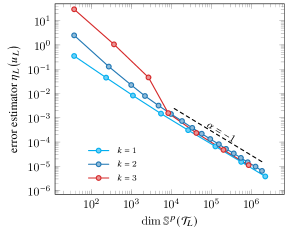
(A)

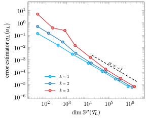
(B)

Figure 7. Optimality of AFEM for jumping diffusion. The convergence history plot of the discretization error estimator $\eta_{L}(u_{L})$ for polynomial degree $p=2$ with respect to the total computational cost for the checkerboard diffusion (left) and the stripe diffusion (right).

	Checkerboard		Stripe
	$p=1$	$p=2$	$p=1$	$p=2$
$k=1$	-0.4961	-0.9877	-0.4956	-1.0116
$k=2$	-0.4960	-0.9946	-0.4969	-0.9670
$k=3$	-0.4960	-0.9826	-0.5095	-0.9766

Table 1. Mean value of experimental convergence rates of the discretization error estimator $\eta_{L}(u_{L})$ over the cumulative cost in a $\log\log$-plot for polynomial degrees $p=1,2$ and diffusion coefficient numbers $k=1,2,3$.

	checkerboard		stripe
	$p=1$	$p=2$	$p=1$	$p=2$
$k=1$	1	1.0455 (mean), 2 (max)	1	1.0455 (mean), 2 (max)
$k=2$	1	2.3261 (mean), 5 (max)	1	1.0417 (mean), 2 (max)
$k=3$	1	1.1818 (mean), 3 (max)	1	1.0833 (mean), 2 (max)

Table 2. Mean and maximal iteration numbers for polynomial degrees $p=1,2$ and diffusion coefficient numbers $k=1,2,3$.

5. Proofs

Below we present proofs of intermediate results leading to our main Theorem 2.4 of $L$- and $p$-robust contraction of the multigrid solver and the $L$- and $p$-robust two-sided bound of the algebraic error by the built-in a posteriori estimator. We emphasize that this result improves the recent work [MPV21] by removing the $L$-dependence. From an algorithmic point of view, this is done by applying local smoothing only on patches which change in the refinement step on lowest-order levels instead of on every patch as was the case in [MPV21]. From an analysis point of view, $L$-robustness is achieved thanks to the strengthened Cauchy–Schwarz inequality on bisection-generated meshes (Proposition 5.12) building on the property that the levelwise overlap of the smoothed patches stays uniformly bounded. The next essential ingredient to prove the main result is an $hp$-stable decomposition on bisection generated meshes (Proposition 5.8), then one combines the results carefully together with the simple but crucial observation of uniform boundedness in the number of overlapping patches for a fixed level (Lemma 5.1) and bounds on the step-sizes and the levelwise solver update (Lemma 5.3).

5.1. Auxiliary results

We start with the simple observation that the number of overlapping patches is uniformly bounded.

Lemma 5.1 (Finite patch overlap).

For all $T\in\mathcal{T}_{\ell}$, there holds

$$\#(\mathcal{V}_{\ell}\cap T)=d+1.$$ (23)

Therefore, for all $q\in\mathbb{N}$, it holds that

$$\Big{|}\!\Big{|}\!\Big{|}\sum\limits_{z\in\mathcal{V}_{\ell}}v_{\ell,z}\Big{|}\!\Big{|}\!\Big{|}^{2}\leq(d+1)\sum\limits_{z\in\mathcal{V}_{\ell}}|\!|\!|v_{\ell,z}|\!|\!|^{2}\quad\text{for all }v_{\ell,z}\in\mathbb{V}_{\ell,z}^{q}.$$ (24)

Similar arguments show that

$$\Big{\|}\nabla\sum\limits_{z\in\mathcal{V}_{\ell}}v_{\ell,z}\Big{\|}^{2}\leq(d+1)\sum\limits_{z\in\mathcal{V}_{\ell}}\|\nabla v_{\ell,z}\|^{2}\quad\text{for all }v_{\ell,z}\in\mathbb{V}_{\ell,z}^{q}.$$ (25)

Proof 5.2.

The overlap (23) is clear from the geometry of the elements in the mesh. For all $\ell=0,\dots,L$, the discrete Cauchy–Schwarz inequality and (23) lead to

$$\Big{|}\!\Big{|}\!\Big{|}\sum\limits_{z\in\mathcal{V}_{\ell}}v_{\ell,z}\Big{|}\!\Big{|}\!\Big{|}^{2}=\sum\limits_{T\in\mathcal{T}_{\ell}}\Big{|}\!\Big{|}\!\Big{|}\sum\limits_{z\in\mathcal{V}_{\ell}\cap T}v_{\ell,z}\Big{|}\!\Big{|}\!\Big{|}_{T}^{2}\leq(d+1)\sum\limits_{z\in\mathcal{V}_{\ell}}|\!|\!|v_{\ell,z}|\!|\!|^{2}.$$

This concludes the proof.

Next, we present bounds on the step-size and the levelwise solver update.

Lemma 5.3.

For all $\ell\in\{1,\dots,L\}$, we have

$$|\!|\!|\lambda_{\ell}\rho_{\ell}|\!|\!|^{2}\leq\lambda_{\ell}\sum\limits_{z\in\mathcal{V}_{\ell}^{+}}|\!|\!|\rho_{\ell,z}|\!|\!|^{2}.$$ (26)

Moreover, we have upper and lower bounds for the step-sizes,

$$\frac{1}{d+1}\leq\lambda_{\ell}\leq{d+1}\quad\text{for all }\ell=1,\dots,L-1\quad\text{and}\quad\frac{1}{d+1}\leq\lambda_{L}.$$ (27)

Proof 5.4.

Step 1: Proof of (26) if $\ell=L$ or $(R_{L}(\rho_{\ell})-\lAngle\sigma_{\ell-1}\,,\,\rho_{\ell}\rAngle)/|\!|\!|\rho_{\ell}|\!|\!|^{2}\leq d+1$ for $\ell\in\{1,\dots,L-1\}$. From Step (ii) of Algorithm 2.3, we have that $\lambda_{\ell}=(R_{L}(\rho_{\ell})-\lAngle\sigma_{\ell-1}\,,\,\rho_{\ell}\rAngle)/|\!|\!|\rho_{\ell}|\!|\!|^{2}$ and thus

$$|\!|\!|\lambda_{\ell}\rho_{\ell}|\!|\!|^{2}\!=\lambda_{\ell}\,\cfrac{R_{L}(\rho_{\ell})-\lAngle\sigma_{\ell-1}\,,\,\rho_{\ell}\rAngle}{|\!|\!|\rho_{\ell}|\!|\!|^{2}}\,|\!|\!|\rho_{\ell}|\!|\!|^{2} =\lambda_{\ell}\sum\limits_{z\in\mathcal{V}_{\ell}^{+}}\left(R_{L}(\rho_{\ell,z})-\lAngle\sigma_{\ell-1}\,,\,\rho_{\ell,z}\rAngle\right)$$

$$\stackrel{{\scriptstyle\mathclap{\eqref{equation:alg_step2}}}}{{=}}~{}\lambda_{\ell}\!\!\sum\limits_{z\in\mathcal{V}_{\ell}^{+}}\!|\!|\!|\rho_{\ell,z}|\!|\!|^{2}.$$

Step 2: Proof of (26) in the remaining cases. We use the finite overlap of the patches in Lemma 5.1 to obtain

$$|\!|\!|\lambda_{\ell}\rho_{\ell}|\!|\!|^{2}=\frac{\lambda_{\ell}}{d+1}|\!|\!|\rho_{\ell}|\!|\!|^{2}\stackrel{{\scriptstyle\eqref{equation:norm_estimate_general}}}{{\leq}}\frac{\lambda_{\ell}}{d+1}(d+1)\sum\limits_{z\in\mathcal{V}_{\ell}^{+}}|\!|\!|\rho_{\ell,z}|\!|\!|^{2}=\lambda_{\ell}\sum\limits_{z\in\mathcal{V}_{\ell}^{+}}|\!|\!|\rho_{\ell,z}|\!|\!|^{2}.$$

Step 3: Proof of (27). For $\ell\in\{1,\dots,L-1\}$, the upper bound is guaranteed by definition of $\lambda_{\ell}$. The lower bound for $\ell\in\{1,\dots,L\}$ is trivial if $\lambda_{\ell}=1/(d+1)$. Otherwise, it is a consequence of the finite patch overlap:

$$\lambda_{\ell} =\frac{R_{L}(\rho_{\ell})-\lAngle\sigma_{\ell-1}\,,\,\rho_{\ell}\rAngle}{|\!|\!|\rho_{\ell}|\!|\!|^{2}}\stackrel{{\scriptstyle\eqref{equation:alg_step2}}}{{=}}\frac{\sum_{z\in\mathcal{V}_{\ell}^{+}}|\!|\!|\rho_{\ell,z}|\!|\!|^{2}}{|\!|\!|\rho_{\ell}|\!|\!|^{2}}\stackrel{{\scriptstyle\eqref{equation:norm_estimate_general}}}{{\geq}}\frac{1}{d+1}.$$

This concludes the proof.

In the next two subsections, we combine existing results from the literature to obtain a multilevel $hp$-robust stable decomposition and a strengthened Cauchy–Schwarz inequality for our setting of bisection-generated meshes. These will be crucial for the proofs of Theorem 2.4 and Corollary 2.5 in Subsection 5.4 below.

5.2. Multilevel hp-robust stable decomposition on NVB-generated meshes

We start by recalling the one-level $p$-robust stable decomposition from Section 3.4 and Section 4.3 in [SMPZ08] for $d=2$ and $d=3$, respectively.

Lemma 5.5 ($p$-robust one level decomposition).

Let $v_{L}\in\mathbb{V}_{L}^{p}$. Then, there exists a decomposition

$$v_{L}=v_{L}^{1}+\sum_{z\in\mathcal{V}_{L}}v^{p}_{L,z}\quad\text{with }v_{L}^{1}\in\mathbb{V}_{L}^{1}\text{ and }v^{p}_{L,z}\in\mathbb{V}_{L,z}^{p},$$ (28)

which is stable in the sense of

$$\|\nabla v_{L}^{1}\|^{2}+\sum_{z\in\mathcal{V}_{L}}\|\nabla v^{p}_{L,z}\|^{2}\leq C_{{\rm OL}}^{2}\|\nabla v_{L}\|^{2}.$$ (29)

The constant $C_{{\rm OL}}$ depends only on the space dimension $d$, the $\gamma$-shape regularity (5), and the quasi-uniformity constant $C_{\rm qu}$ from (6).

Similarly, we recall the local multilevel decomposition for piecewise affine functions proven in [WZ17, Lemma 3.1]. In order to present this stable decomposition in a form that is more suitable for our forthcoming analysis, we add a short proof for completeness.

Lemma 5.6 ($h$-robust local multilevel decomposition for lowest-order functions).

Let $v_{L}^{1}\in\mathbb{V}_{L}^{1}$. Then, there exists a decomposition

$$v_{L}^{1}=\sum_{\ell=0}^{L}\sum_{z\in\mathcal{V}_{\ell}^{+}}v^{1}_{\ell,z}\quad\text{with }v^{1}_{\ell,z}\in\mathbb{V}^{1}_{\ell,z},$$ (30)

which is stable in the sense of

$$\sum_{\ell=0}^{L}\sum_{z\in\mathcal{V}_{\ell}^{+}}\|\nabla v^{1}_{\ell,z}\|^{2}\leq C_{{\rm ML}}^{2}\|\nabla v_{L}^{1}\|^{2}.$$ (31)

The constant $C_{{\rm ML}}$ depends only on the space dimension $d$, the $\gamma$-shape regularity (5), and the quasi-uniformity constant $C_{\rm qu}$ from (6).

Proof 5.7.

Let $v_{L}^{1}\in\mathbb{V}_{L}^{1}$. Define $w_{\ell}^{1}\coloneqq(\Pi_{\ell}-\Pi_{\ell-1})v_{L}^{1}$ for $\ell\in\{0,\dots,L\}$, where $\Pi_{-1}\coloneqq 0$ and $\Pi_{\ell}$ is the projection to $\mathbb{V}_{\ell}^{1}$ from [WZ17, Section 3]. From [WZ17, Lemma 3.1], it holds that $w_{\ell}^{1}\in{\rm span}\big{\{}\varphi_{\ell,z}\,:\,z\in\mathcal{V}_{\ell}^{+}\big{\}}$ with $\varphi_{\ell,z}$ being the $\mathbb{S}^{1}(\mathcal{T}_{\ell})$ hat-function at vertex $z\in\mathcal{V}_{\ell}$. We decompose $w_{\ell}^{1}=\sum_{z\in\mathcal{V}_{\ell}^{+}}v_{\ell,z}^{1}$ with $v_{\ell,z}^{1}:=w_{\ell}^{1}(z)\varphi_{\ell,z}\in\mathbb{V}^{1}_{\ell,z}$ and thus obtain

$$v_{L}^{1}=\sum_{\ell=0}^{L}(\Pi_{\ell}-\Pi_{\ell-1})v_{L}^{1}=\sum_{\ell=0}^{L}w_{\ell}^{1}=\sum_{\ell=0}^{L}\sum_{z\in\mathcal{V}_{\ell}^{+}}v^{1}_{\ell,z}.$$ (32)

For fixed $\ell$ and $z\in\mathcal{V}_{\ell}^{+}$, the equivalence of norms on finite-dimensional spaces proves

$$\begin{split}\|v^{1}_{\ell,z}\|_{\omega_{\ell,z}}&\leq\sum_{T\in{\mathcal{T}_{\ell,z}}}\|w^{1}_{\ell}(z)\varphi_{\ell,z}\|_{T}\\ &\leq\!\!\sum_{T\in{\mathcal{T}_{\ell,z}}}\|w_{\ell}^{1}\|_{L^{\infty}(T)}|T|^{1/2}\lesssim\sum_{T\in{\mathcal{T}_{\ell,z}}}\|w_{\ell}^{1}\|_{T}\simeq\|w_{\ell}^{1}\|_{\omega_{\ell,z}},\end{split}$$ (33)

where the hidden constants depend only on $\gamma$-shape regularity (5). To obtain stability of the decomposition (32), we use an inverse inequality on the patches and the stability proved in [WZ17, Lemma 3.7]:

$$\sum_{\ell=0}^{L}\sum_{z\in\mathcal{V}_{\ell}^{+}}\|\nabla v^{1}_{\ell,z}\|^{2} \lesssim\sum_{\ell=0}^{L}\sum_{z\in\mathcal{V}_{\ell}^{+}}h_{\ell,z}^{-2}\|v^{1}_{\ell,z}\|^{2}_{\omega_{\ell,z}}\stackrel{{\scriptstyle\eqref{equation:loc_nd_L2}}}{{\lesssim}}\sum_{\ell=0}^{L}\sum_{z\in\mathcal{V}_{\ell}^{+}}h_{\ell,z}^{-2}\|w^{1}_{\ell}\|^{2}_{\omega_{\ell,z}}$$

$$=\sum_{\ell=0}^{L}\sum_{z\in\mathcal{V}_{\ell}^{+}}h_{\ell,z}^{-2}\|(\Pi_{\ell}-\Pi_{\ell-1})v_{L}^{1}\|^{2}_{\omega_{\ell,z}}\stackrel{{\scriptstyle\text{\cite[cite]{[\@@bibref{}{Wu_Zheng_Multigrid}{}{}]}}}}{{\lesssim}}\|\nabla v_{L}^{1}\|^{2}.$$

This concludes the proof.

The combination of the two previous lemmas, done similarly in [MPV20, Proposition 7.6] for a non-local and hence not $h$-robust solver, leads to the following $hp$-robust decomposition.

Proposition 5.8 ($hp$-robust local multilevel decomposition).

Let $v_{L}\in\mathbb{V}_{L}^{p}$. Then, there exist $v_{0}\in\mathbb{V}_{0}^{1},\ v_{\ell,z}\in\mathbb{V}_{\ell,z}^{1}$, and $v_{L,z}\in\mathbb{V}_{L,z}^{p}$ such that

$$v_{L}=v_{0}+\sum_{\ell=1}^{L-1}\sum_{z\in\mathcal{V}_{\ell}^{+}}v_{\ell,z}+\sum_{z\in\mathcal{V}_{L}}v_{L,z}.$$ (34)

and this decomposition is stable in the sense of

$$|\!|\!|v_{0}|\!|\!|^{2}+\sum_{\ell=1}^{L-1}\sum_{z\in\mathcal{V}_{\ell}^{+}}|\!|\!|v_{\ell,z}|\!|\!|^{2}+\sum_{z\in\mathcal{V}_{L}}|\!|\!|v_{L,z}|\!|\!|^{2}\leq C^{2}_{{\rm SD}}|\!|\!|v_{L}|\!|\!|^{2}.$$ (35)

The constant $C_{{\rm SD}}\geq 1$ depends only on the space dimension $d$, $\gamma$-shape regularity (5), the quasi-uniformity constant $C_{\rm qu}$ from (6), and the ratio of $\Lambda_{\max}$ and $\Lambda_{\min}$.

Proof 5.9.

Let $v_{L}\in\mathbb{V}^{p}_{L}$. We begin with the decomposition of $v_{L}$ by (28), then continue with the further decomposition of the lowest-order contribution $v_{L}^{1}$ in a multilevel way (30):

$$v_{L}\stackrel{{\scriptstyle\eqref{equation:one_level_p_decomposition}}}{{=}}v_{L}^{1}+\sum_{z\in\mathcal{V}_{L}}v^{p}_{L,z} \stackrel{{\scriptstyle\eqref{equation:multilevel_local_lowest_order_decomposition}}}{{=}}\sum_{\ell=0}^{L}\sum_{z\in\mathcal{V}_{\ell}^{+}}v^{1}_{\ell,z}+\sum_{z\in\mathcal{V}_{L}}v^{p}_{L,z}$$

$$=\sum_{z\in\mathcal{V}_{0}}v^{1}_{0,z}+\sum_{\ell=1}^{L-1}\sum_{z\in\mathcal{V}_{\ell}^{+}}v^{1}_{\ell,z}+\sum_{z\in\mathcal{V}_{L}^{+}}v^{1}_{L,z}+\sum_{z\in\mathcal{V}_{L}}v_{L,z}^{p}.$$

By defining $v_{0}:=\sum_{z\in\mathcal{V}_{0}}v^{1}_{0,z}\in\mathbb{V}_{0}^{1}$, $v_{\ell,z}:=v^{1}_{\ell,z}\in\mathbb{V}_{\ell,z}^{1}$ for $z\in\mathcal{V}_{\ell}^{+}$ and $1\leq\ell\leq L-1$, and $v_{L,z}:=v^{1}_{L,z}+v^{p}_{L,z}\in\mathbb{V}_{L,z}^{p}$ for $z\in\mathcal{V}_{L}^{+}$ and $v_{L,z}:=v^{p}_{L,z}\in\mathbb{V}_{L,z}^{p}$ for $z\in\mathcal{V}_{L}\setminus\mathcal{V}_{L}^{+}$, we obtain the decomposition (34). It remains to show that this decomposition is stable (35). First, we have for the coarsest level that

$$\|\nabla v_{0}\|^{2}\stackrel{{\scriptstyle\eqref{equation:norm_estimate_special}}}{{\leq}}(d+1)\sum_{z\in\mathcal{V}_{0}}\|\nabla v^{1}_{0,z}\|^{2}.$$

For the finest level, it holds that

$$\sum_{z\in\mathcal{V}_{L}}\|\nabla v_{L,z}\|^{2} \leq\sum_{z\in\mathcal{V}_{L}\backslash\mathcal{V}_{L}^{+}}\|\nabla v^{p}_{L,z}\|^{2}+2\,\sum_{z\in\mathcal{V}_{L}}\bigl{(}\|\nabla v^{1}_{L,z}\|^{2}+\|\nabla v^{p}_{L,z}\|^{2}\bigr{)}$$

$$\leq(d+1)\sum_{z\in\mathcal{V}_{L}^{+}}\|\nabla v^{1}_{L,z}\|^{2}+(d+1)\sum_{z\in\mathcal{V}_{L}}\|\nabla v^{p}_{L,z}\|^{2}.$$

A combination of the two estimates shows that

$$\|\nabla v_{0}\|^{2}+\sum_{\ell=1}^{L-1}\sum_{z\in\mathcal{V}_{\ell}^{+}}\|\nabla v_{\ell,z}\|^{2}+\sum_{z\in\mathcal{V}_{L}}\|\nabla v_{L,z}\|^{2}$$

$$\leq(d+1)\Big{(}\sum_{z\in\mathcal{V}_{0}}\|\nabla v^{1}_{0,z}\|^{2}+\sum_{\ell=1}^{L-1}\!\sum_{z\in\mathcal{V}_{\ell}^{+}}\!\|\nabla v^{1}_{\ell,z}\|^{2}+\sum_{z\in\mathcal{V}_{L}^{+}}\|\nabla v^{1}_{L,z}\|^{2}+\sum_{z\in\mathcal{V}_{L}}\|\nabla v^{p}_{L,z}\|^{2}\Big{)}$$

$$\leq(d+1)\sum_{\ell=0}^{L}\sum_{z\in\mathcal{V}_{\ell}^{+}}\|\nabla v^{1}_{\ell,z}\|^{2}+(d+1)\sum_{z\in\mathcal{V}_{L}}\|\nabla v^{p}_{L,z}\|^{2}$$

$$\stackrel{{\scriptstyle\mathclap{\eqref{equation:multilevel_local_lowest_order_stability}}}}{{\leq}}C_{{\rm ML}}^{2}(d+1)\|\nabla v^{1}_{L}\|^{2}+(d+1)\sum_{z\in\mathcal{V}_{L}}\|\nabla v^{p}_{L,z}\|^{2}$$

$$\stackrel{{\scriptstyle\mathclap{\eqref{equation:one_level_p_stability}}}}{{\leq}}\max\{1,C_{{\rm ML}}^{2}\}C_{{\rm OL}}^{2}(d+1)\|\nabla v_{L}\|^{2}.$$

Hence, the decomposition (34) is stable with $(C_{{\rm SD}}^{\prime})^{2}\coloneqq\max\{1,C_{{\rm ML}}^{2}\}C_{{\rm OL}}^{2}(d+1)$ with respect to the $H^{1}(\Omega)$-seminorm. Taking into account the variations of the diffusion coefficient $\bm{K}$, we obtain (35) with the stability constant $C_{{\rm SD}}\coloneqq C_{{\rm SD}}^{\prime}\Lambda_{\max}/\Lambda_{\min}$.

5.3. Strengthened Cauchy–Schwarz inequality on NVB-generated meshes

The following results are proved in the spirit of [HWZ12, CNX12]. Note that the setting of this work is similar to [HWZ12], and unlike [CNX12], the underlying adaptive meshes of the space hierarchy are not restricted to one bisection per level.

For analysis purposes, we introduce a sequence of uniformly refined triangulations indicated by $\{\widehat{\mathcal{T}}_{j}\}_{j=0}^{M}$ such that $\widehat{\mathcal{T}}_{j+1}\coloneqq\texttt{refine}(\widehat{\mathcal{T}}_{j},\widehat{\mathcal{T}}_{j})$ and $\widehat{\mathcal{T}}_{0}=\mathcal{T}_{0}$, where $\mathtt{refine}$ enforces one bisection per element. According to [Ste08], admissibility of $\mathcal{T}_{0}$ ensures that indeed each element $T\in\widehat{\mathcal{T}}_{j}$ is bisected only once into two children $T^{\prime},T^{\prime\prime}\in\widehat{\mathcal{T}}_{j+1}$. In the following, we will indicate the equivalent notation to Section 2 on uniform triangulations $\widehat{\mathcal{T}}_{j}$ with a hat, e.g., $\widehat{\mathbb{V}}_{j}^{1}$ is the equivalent of $\mathbb{V}_{\ell}^{1}$ on the uniformly refined mesh $\widehat{\mathcal{T}}_{j}$. The connection of the uniformly refined meshes and their adaptively generated counterpart requires further notation. For a given level $0\leq\ell\leq L$ and a given node $z\in\mathcal{V}_{\ell}$, we define the generation $g_{\ell,z}$ of the patch by the maximum number of times an element of the patch has been bisected

$$g_{\ell,z}:=\max_{T\in\mathcal{T}_{\ell,z}}\log_{2}(|T_{0}|/|T|)\in\mathbb{N}_{0},$$ (36)

where $T_{0}\in\mathcal{T}_{0}$ denotes the unique ancestor element of $T\in\mathcal{T}_{\ell}$. Define the maximal generation $M=\max_{z\in\mathcal{V}_{L}}g_{L,z}$.

First, we present the following result for uniformly refined meshes and then exploit this for our setting of adaptively refined meshes.

Lemma 5.10 (Strengthened Cauchy–Schwarz on nested uniform meshes).

Let $0\leq i\leq j\leq M$, and $\widehat{u}_{i}\in\widehat{\mathbb{V}}_{i}^{1}$ as well as $\widehat{v}_{j}\in\widehat{\mathbb{V}}_{j}^{1}$. Then, it holds that

$$\lAngle\widehat{u}_{i}\,,\,\widehat{v}_{j}\rAngle\leq\widehat{C}_{\rm SCS}\,\delta^{j-i}\widehat{h}_{j}^{-1}\big{\|}\nabla\widehat{u}_{i}\big{\|}\big{\|}\widehat{v}_{j}\big{\|},$$ (37)

where $\delta=2^{-1/2}$ and $\widehat{C}_{\rm SCS}>0$ depends only on the domain $\Omega$, the initial triangulation $\mathcal{T}_{0}$, $\Lambda_{\max}$, $\max_{T\in\widehat{\mathcal{T}}_{M}}\|\operatorname{\mathrm{div}}(\bm{K})\|_{L^{\infty}(T)}$, and $\gamma$-shape regularity from (5).

Proof 5.11.

We begin by splitting the domain $\Omega$ into elementwise components, applying integration by parts, and using the Cauchy–Schwarz inequality. Note that the restriction of $\widehat{u}_{i}$ to any element $T\in\widehat{\mathcal{T}}_{i}$ is an affine function, and hence the second derivatives vanish. Thus, it holds with the outer normal $\bm{n}$ to $\partial T$ that

$$\lAngle\widehat{u}_{i}\,,\,\widehat{v}_{j}\rAngle =\sum_{T\in\widehat{\mathcal{T}}_{i}}\int_{T}\bm{K}\nabla\widehat{u}_{i}\cdot\nabla\widehat{v}_{j}\,{\rm d}{x}$$

$$=\sum_{T\in\widehat{\mathcal{T}}_{i}}\Big{(}-\int_{T}{\rm div}(\bm{K}\nabla\widehat{u}_{i})\widehat{v}_{j}\,{\rm d}{x}+\int_{\partial T}\bm{K}\nabla\widehat{u}_{i}\cdot\bm{n}\,\widehat{v}_{j}\,{\rm d}{x}\Big{)}$$

$$\leq\sum_{T\in\widehat{\mathcal{T}}_{i}}\Big{(}\big{\|}({\rm div}\bm{K})\cdot\nabla\widehat{u}_{i}\big{\|}_{L^{2}(T)}\big{\|}\widehat{v}_{j}\big{\|}_{L^{2}(T)}+\big{\|}\bm{K}\nabla\widehat{u}_{i}\big{\|}_{L^{2}(\partial T)}\big{\|}\widehat{v}_{j}\big{\|}_{L^{2}(\partial T)}\Big{)}.$$

Due to $\bm{K}\in W^{1,\infty}(T)$, the fact that $\widehat{u}_{i},\widehat{v}_{j}$ are piecewise affine, a discrete trace inequality, and $\widehat{h}_{i}^{-1}\gtrsim 1$, we get

$$\lAngle\widehat{u}_{i}\,,\,\widehat{v}_{j}\rAngle \lesssim\sum_{T\in\widehat{\mathcal{T}}_{i}}\Big{(}\big{\|}\nabla\widehat{u}_{i}\big{\|}_{L^{2}(T)}\big{\|}\widehat{v}_{j}\big{\|}_{L^{2}(T)}+\big{\|}\nabla\widehat{u}_{i}\big{\|}_{L^{2}(\partial T)}\big{\|}\widehat{v}_{j}\big{\|}_{L^{2}(\partial T)}\Big{)}$$

$$\lesssim\sum_{T\in\widehat{\mathcal{T}}_{i}}\Big{(}\big{\|}\nabla\widehat{u}_{i}\big{\|}_{L^{2}(T)}\big{\|}\widehat{v}_{j}\big{\|}_{L^{2}(T)}+\bigl{(}\widehat{h}_{i}^{-1/2}\big{\|}\nabla\widehat{u}_{i}\big{\|}_{L^{2}(T)}\bigr{)}\,\bigl{(}\widehat{h}_{i}^{-1/2}\big{\|}\widehat{v}_{j}\big{\|}_{L^{2}(T)}\bigr{)}\Big{)}$$

$$=\sum_{T\in\widehat{\mathcal{T}}_{i}}\bigl{(}1+h_{i}^{-1}\bigr{)}\,\big{\|}\nabla\widehat{u}_{i}\big{\|}_{L^{2}(T)}\big{\|}\widehat{v}_{j}\big{\|}_{L^{2}(T)}$$

$$\lesssim\sum_{T\in\widehat{\mathcal{T}}_{i}}\widehat{h}_{i}^{-1}\big{\|}\nabla\widehat{u}_{i}\big{\|}_{L^{2}(T)}\big{\|}\widehat{v}_{j}\big{\|}_{L^{2}(T)}.$$

Moreover, note that due to uniform refinement, we have equivalence $\delta^{j-i}=(2^{-1/2})^{j-i}\simeq\big{(}\widehat{h}_{j}/\widehat{h}_{i}\big{)}^{1/2}$ and $\widehat{h}_{j}\leq\widehat{h}_{i}$. Using the last equation multiplied by $1=\widehat{h}_{j}^{1/2}\,\widehat{h}_{j}^{-1/2}$, we derive that

$$\lAngle\widehat{u}_{i}\,,\,\widehat{v}_{j}\rAngle \lesssim\sum_{T\in\widehat{\mathcal{T}}_{i}}\Big{(}\cfrac{\widehat{h}_{j}}{\widehat{h}_{i}}\Big{)}^{1/2}\,\widehat{h}_{i}^{-1/2}\,\widehat{h}_{j}^{-1/2}\big{\|}\nabla\widehat{u}_{i}\big{\|}_{L^{2}(T)}\big{\|}\widehat{v}_{j}\big{\|}_{L^{2}(T)}$$

$$\lesssim\sum_{T\in\widehat{\mathcal{T}}_{i}}\delta^{j-i}\,\widehat{h}_{j}^{-1}\,\big{\|}\nabla\widehat{u}_{i}\big{\|}_{L^{2}(T)}\big{\|}\widehat{v}_{j}\big{\|}_{L^{2}(T)}\leq\widehat{h}_{j}^{-1}\delta^{j-i}\big{\|}\nabla\widehat{u}_{i}\big{\|}_{L^{2}(\Omega)}\big{\|}\widehat{v}_{j}\big{\|}_{L^{2}(\Omega)}.$$

This concludes the proof.

The last result enables us to tackle the setting of adaptively-refined meshes.

Proposition 5.12 (Strengthened Cauchy–Schwarz on nested adaptive meshes).

Consider levelwise functions $v_{\ell}=\sum_{z\in\mathcal{V}_{\ell}^{+}}v_{\ell,z}^{1}\in\mathbb{V}_{\ell}^{1}$ with $v_{\ell,z}^{1}\in\mathbb{V}_{\ell,z}^{1}$ for all $1\leq\ell\leq L-1$. Then, it holds that

$$\sum_{\ell=1}^{L-1}\sum_{k=1}^{\ell-1}\lAngle v_{k}\,,\,v_{\ell}\rAngle\leq C_{\rm SCS}\Big{(}\sum_{k=1}^{L-2}\sum_{w\in\mathcal{V}_{k}^{+}}|\!|\!|v_{k,w}^{1}|\!|\!|^{2}\Big{)}^{1/2}\Big{(}\sum_{\ell=1}^{L-1}\sum_{z\in\mathcal{V}_{\ell}^{+}}|\!|\!|v_{\ell,z}^{1}|\!|\!|^{2}\Big{)}^{1/2},$$ (38)

where $C_{\rm SCS}>0$ depends only on $\Omega$, the initial triangulation $\mathcal{T}_{0}$, $\Lambda_{\max}/\Lambda_{\min}$, $\max_{T\in\mathcal{T}_{L}}\|\operatorname{\mathrm{div}}(\bm{K})\|_{L^{\infty}(T)}/\Lambda_{\min}$, and $\gamma$-shape regularity (5).

Proof 5.13.

Let $M\in\mathbb{N}$. The proof consists of five steps.

Step 1. First note that, for any $0<\delta<1$ and $x_{i},y_{i}>0$ with $0\leq i\leq M$, there holds

$$\sum_{i=0}^{M}\sum_{j=i}^{M}\delta^{j-i}x_{i}y_{j}\leq\frac{1}{1-\delta}\Big{(}\sum_{i=0}^{M}x_{i}^{2}\Big{)}^{1/2}\Big{(}\sum_{j=0}^{M}y_{j}^{2}\Big{)}^{1/2}.$$ (39)

To see this, we change the summation order accordingly and use the Cauchy–Schwarz inequality to obtain

$$\sum_{i=0}^{M}\sum_{j=i}^{M}\, \delta^{j-i}x_{i}y_{j}=\!\sum_{i=0}^{M}\sum_{m=0}^{M-i}\delta^{m}x_{i}y_{m+i}=\sum\limits_{m=0}^{M}\sum\limits_{i=0}^{M-m}\delta^{m}x_{i}y_{m+i}$$

$$\leq\sum_{m=0}^{M}\delta^{m}\,\Big{[}\big{(}\sum_{i=0}^{M-m}x_{i}^{2}\big{)}^{1/2}\big{(}\sum_{i=0}^{M-m}y_{m+i}^{2}\big{)}^{1/2}\Big{]}\leq\Big{(}\sum_{m=0}^{M}\delta^{m}\Big{)}\Big{(}\sum_{i=0}^{M}x_{i}^{2}\Big{)}^{1/2}\Big{(}\sum_{j=0}^{M}y_{j}^{2}\Big{)}^{1/2}.$$

The geometric series then proves the claim (39).

Step 2. Let $z\in\mathcal{V}_{L}$ and $0\leq j\leq M$ and recall the patch generation $g_{\ell,z}$ from (36). We introduce the set

$$\mathscr{L}_{\underline{\ell},\overline{\ell}}(z,j):=\{\ell\in\{\underline{\ell},\ldots,\overline{\ell}\}:z\in\mathcal{V}_{\ell}^{+}\text{ and }g_{\ell,z}=j\}\quad\text{with }0\leq\underline{\ell}\leq\overline{\ell}\leq L.$$ (40)

This set allows to track how large the levelwise overlap of patches with the same generation is. Crucially, the cardinality of these sets is uniformly bounded by

$$\max_{\begin{subarray}{c}z\in\mathcal{V}_{L}\\ 0\leq j\leq M\end{subarray}}\#(\mathscr{L}_{0,L}(z,j))\leq C_{\mathrm{lev}}<\infty;$$ (41)

see, e.g., [WC06, Lemma 3.1] in the two-dimensional setting with arguments that transfer to three dimensions. The constant $C_{\mathrm{lev}}$ solely depends on $\gamma$-shape regularity (5).

Step 3. We introduce a way to reorder the patch contributions by generations (36). Note that, for any $0\leq j\leq M$, $1\leq\ell\leq L-1$, and $z\in\mathcal{V}_{\ell}^{+}$ such that $g_{\ell,z}=j$, the patch contribution $v_{\ell,z}^{1}\in\mathbb{V}_{\ell,z}^{1}$ also belongs to $\widehat{\mathbb{V}}_{j}^{1}$. Once the generation constraint is introduced, one can shift the perspective from summing over “adaptive” levels and associated vertices to summing over “uniform” vertices and only the (finitely many, cf. (41)) levels where each vertex satisfies the generation constraint, i.e., for $0\leq\underline{\ell}\leq\overline{\ell}\leq L$ and $0\leq j\leq M$, the two following sets coincide

$$\begin{split}\big{\{}(\ell,z)\in\mathbb{N}_{0}\times\mathcal{V}_{L}\,:\,\ell\in&\{\underline{\ell},\ldots,\overline{\ell}\},z\in\mathcal{V}_{\ell}^{+}\text{ with }g_{\ell,z}=j\big{\}}\\ &=\big{\{}(\ell,z)\in\mathbb{N}_{0}\times\mathcal{V}_{L}\,:\,z\in\widehat{\mathcal{V}}_{j},\ell\in\!{\mathscr{L}}_{\underline{\ell},\overline{\ell}}(z,j)\big{\}}.\end{split}$$ (42)

Step 4. According to $\gamma$-shape regularity (5), all elements in the patch have comparable size depending on $C_{\mathrm{qu}}$ from (6). If $g_{\ell,z}=j$, (at least) one element $T^{\star}\in\mathcal{T}_{\ell,z}$ satisfies $T^{\star}\in\widehat{\mathcal{T}}_{j}$ and it follows that $\widehat{h}_{j}\simeq|T^{\star}|^{1/d}\simeq|\omega_{\ell,z}|^{1/d}\simeq h_{\ell,z}.$ In particular, there exists $C_{\rm eq}>0$ such that

$$\widehat{h}_{j}^{-1}\leq C_{\rm eq}h_{\ell,z}^{-1}.$$ (43)

Step 5. We proceed to prove the main estimate (38). The central feature of the following approach is to introduce additional sums over the generations with generation constraints, i.e., there holds for every admissible $\ell,k$, that

$$\lAngle v_{k}\,,\,v_{\ell}\rAngle =\sum_{z\in\mathcal{V}_{\ell}^{+}}\sum_{w\in\mathcal{V}_{k}^{+}}\lAngle v_{k,w}^{1}\,,\,v_{\ell,z}^{1}\rAngle=\sum_{j=0}^{M}\sum_{i=0}^{M}\sum_{\begin{subarray}{c}z\in\mathcal{V}_{\ell}^{+}\\ g_{\ell,z}=j\end{subarray}}\sum_{\begin{subarray}{c}w\in\mathcal{V}_{k}^{+}\\ g_{k,w}=i\end{subarray}}\lAngle v_{k,w}^{1}\,,\,v_{\ell,z}^{1}\rAngle$$

$$=\sum_{j=0}^{M}\sum_{i=0}^{j}\sum_{\begin{subarray}{c}z\in\mathcal{V}_{\ell}^{+}\\ g_{\ell,z}=j\end{subarray}}\sum_{\begin{subarray}{c}w\in\mathcal{V}_{k}^{+}\\ g_{k,w}=i\end{subarray}}\lAngle v_{k,w}^{1}\,,\,v_{\ell,z}^{1}\rAngle+\sum_{j=0}^{M}\sum_{i=j+1}^{M}\sum_{\begin{subarray}{c}z\in\mathcal{V}_{\ell}^{+}\\ g_{\ell,z}=j\end{subarray}}\sum_{\begin{subarray}{c}w\in\mathcal{V}_{k}^{+}\\ g_{k,w}=i\end{subarray}}\lAngle v_{k,w}^{1}\,,\,v_{\ell,z}^{1}\rAngle.$$

We abbreviate the terms as $S_{1}(\ell,k)$ and $S_{2}(\ell,k)$, respectively. A change of the summation of order $i$ and $j$ yields for $S_{1}(\ell,k)$ that

$$S_{1}(\ell,k)=\sum_{i=0}^{M}\sum_{j=i}^{M}\sum_{\begin{subarray}{c}z\in\mathcal{V}_{\ell}^{+}\\ g_{\ell,z}=j\end{subarray}}\sum_{\begin{subarray}{c}w\in\mathcal{V}_{k}^{+}\\ g_{k,w}=i\end{subarray}}\lAngle v_{k,w}^{1}\,,\,v_{\ell,z}^{1}\rAngle.$$

Summing $S_{2}(\ell,k)$ over all $\ell$ and $k$ and changing the order of summation, we obtain

$$\sum\limits_{\ell=1}^{L-1}\sum\limits_{k=1}^{\ell-1}S_{2}(\ell,k)=\sum_{j=0}^{M}\sum_{i=j+1}^{M}\sum_{k=1}^{L-2}\sum_{\ell=k+1}^{L-1}\sum_{\begin{subarray}{c}z\in\mathcal{V}_{\ell}^{+}\\ g_{\ell,z}=j\end{subarray}}\sum_{\begin{subarray}{c}w\in\mathcal{V}_{k}^{+}\\ g_{k,w}=i\end{subarray}}\lAngle v_{k,w}^{1}\,,\,v_{\ell,z}^{1}\rAngle.$$

Combining these two identities with (42), we see that

$$\sum\limits_{\ell=1}^{L-1}\sum\limits_{k=1}^{\ell-1}\Big{(}S_{1}(\ell,k)+S_{2}(\ell,k)\Big{)} =\sum_{i=0}^{M}\sum_{j=i}^{M}\sum_{\ell=1}^{L-1}\Big{\lAngle}\sum_{\begin{subarray}{c}w\in\widehat{\mathcal{V}}_{i}\end{subarray}}\sum_{k\in\mathscr{L}_{1,\ell-1}(w,i)}\!\!\!v_{k,w}^{1}\,,\,\sum_{\begin{subarray}{c}z\in\mathcal{V}_{\ell}^{+}\\ g_{\ell,z}=j\end{subarray}}\!\!v_{\ell,z}^{1}\Big{\rAngle}$$

$$\quad+\sum_{j=0}^{M}\sum_{i=j+1}^{M}\sum_{k=1}^{L-2}\Big{\lAngle}\sum_{\begin{subarray}{c}w\in\mathcal{V}_{k}^{+}\\ g_{k,w}=i\end{subarray}}\!\!v_{k,w}^{1}\,,\,\sum_{\begin{subarray}{c}z\in\widehat{\mathcal{V}}_{j}\end{subarray}}\sum_{\ell\in\mathscr{L}_{k+1,L-1}(z,j)}\!\!\!v_{\ell,z}^{1}\Big{\rAngle}.$$

We define the last two terms as $S_{1}$ and $S_{2}$, respectively. Since the second term $S_{2}$ is treated in the same way, we only present detailed estimations of the first term $S_{1}$. The strengthened Cauchy–Schwarz inequality (37) for functions defined on uniform meshes followed by the patch overlap (24) leads to

$$S_{1}\leq\widehat{C}_{\rm SCS}\sum_{i=0}^{M}\sum_{j=i}^{M}\delta^{j-i}\sum_{\ell=1}^{L-1}\Big{(}(d+1)\sum_{w\in\widehat{\mathcal{V}}_{i}}\big{\|}\!\!\!\sum_{k\in\mathscr{L}_{1,\ell-1}(w,i)}\!\!\!\nabla v_{k,w}^{1}\big{\|}^{2}\Big{)}^{1/2}\sum_{\begin{subarray}{c}z\in\mathcal{V}_{\ell}^{+}\\ g_{\ell,z}=j\end{subarray}}\widehat{h}_{j}^{-1}\big{\|}v_{\ell,z}^{1}\big{\|}.$$

The identity (42) and the finite levelwise overlap (41) show

$$\sum_{w\in\widehat{\mathcal{V}}_{i}}\big{\|}\!\!\!\sum_{k\in\mathscr{L}_{1,\ell-1}(w,i)}\!\!\!\!\!\!\!\!\!\!\nabla v_{k,w}^{1}\big{\|}^{2}\leq\sum_{k=1}^{\ell-1}\sum_{\begin{subarray}{c}w\in\mathcal{V}_{k}^{+}\\ g_{k,w}=i\end{subarray}}\!\!\!\#(\mathscr{L}_{1,\ell-1}(w,i))\big{\|}\nabla v_{k,w}^{1}\big{\|}^{2}\!\leq C_{\mathrm{lev}}\!\!\sum_{k=1}^{L-2}\sum_{\begin{subarray}{c}w\in\mathcal{V}_{k}^{+}\\ g_{k,w}=i\end{subarray}}\!\!\big{\|}\nabla v_{k,w}^{1}\big{\|}^{2}\!\!.$$

The equivalence of mesh sizes from (43) and a Poincaré-inequality prove

$$\sum_{\ell=1}^{L-1}\sum_{\begin{subarray}{c}z\in\mathcal{V}_{\ell}^{+}\\ g_{\ell,z}=j\end{subarray}}\widehat{h}_{j}^{-1}\big{\|}v_{\ell,z}^{1}\big{\|}\leq C_{\rm eq}C_{\rm P}\sum_{\ell=1}^{L-1}\!\!\sum_{\begin{subarray}{c}z\in\mathcal{V}_{\ell}^{+}\\ g_{\ell,z}=j\end{subarray}}\big{\|}\nabla v_{\ell,z}^{1}\big{\|}.$$

A combination of (42) with (25) and (41), followed again by (42), yields

$$\Bigl{(}\sum_{\ell=1}^{L-1}\!\!\sum_{\begin{subarray}{c}z\in\mathcal{V}_{\ell}^{+}\\ g_{\ell,z}=j\end{subarray}}\!\!\big{\|}\nabla v_{\ell,z}^{1}\big{\|}\Bigr{)}^{2}=\Big{(}\sum_{\begin{subarray}{c}z\in\widehat{\mathcal{V}}_{j}\end{subarray}}\!\sum_{\ell\in\mathscr{L}_{1,L-1}({\color[rgb]{1,0,0}z,j})}\!\!\!\!\!\!\!\!\big{\|}\nabla v_{\ell,z}^{1}\big{\|}\Big{)}^{2}\leq(d+1)\,C_{\mathrm{lev}}\sum_{\ell=1}^{L-1}\sum_{\begin{subarray}{c}z\in\mathcal{V}_{\ell}^{+}\\ g_{\ell,z}=j\end{subarray}}\!\!\big{\|}\nabla v_{\ell,z}^{1}\big{\|}^{2}.$$

Thus, we obtain the bound

$$\sum_{\ell=1}^{L-1}\!\!\sum_{\begin{subarray}{c}z\in\mathcal{V}_{\ell}^{+}\\ g_{\ell,z}=j\end{subarray}}\!\!\big{\|}\nabla v_{\ell,z}^{1}\big{\|}\leq(d+1)^{1/2}C_{\mathrm{lev}}^{1/2}\,\Bigl{(}\sum_{\ell=1}^{L-1}\sum_{\begin{subarray}{c}z\in\mathcal{V}_{\ell}^{+}\\ g_{\ell,z}=j\end{subarray}}\!\!\big{\|}\nabla v_{\ell,z}^{1}\big{\|}^{2}\Bigr{)}^{1/2}$$

Combining all estimates, together with the geometric series bound (39), confirms

$$S_{1}\leq\widehat{C}_{\rm SCS}(d+1)C_{\mathrm{lev}}C_{\rm eq}C_{\rm P}\frac{1}{1-\delta}\Big{(}\sum_{k=1}^{L-2}\sum_{w\in\mathcal{V}_{k}^{+}}\big{\|}\nabla v_{k,w}^{1}\big{\|}^{2}\Big{)}^{1/2}\Big{(}\sum_{\ell=1}^{L-1}\sum_{z\in\mathcal{V}_{\ell}^{+}}\big{\|}\nabla v_{\ell,z}^{1}\big{\|}^{2}\Big{)}^{1/2}.$$

Finally, the result (38) is obtained after summing together with the analogous estimations coming from the remaining term $S_{2}$ and taking into consideration the variations of the diffusion coefficient $\bm{K}$ so that the result holds for the energy norm. This concludes the proof.

5.4. Proof of the main results

For the sake of a concise presentation, we only consider the case $p>1$. The case $p=1$ is already covered in the literature [CNX12, WZ17] and follows from our proof with only minor modifications.

Proof 5.14 (Proof of Theorem 2.4, connection of solver and estimator (12)).

The proof consists of two steps.

Step 1. We show that there holds the identity

$$\begin{split}\Big{|}\!\Big{|}\!\Big{|}\sum_{\ell=0}^{L-1}\lambda_{\ell}\rho_{\ell}\Big{|}\!\Big{|}\!\Big{|}^{2}-2\Big{\lAngle}u_{L}^{\star}-v_{L}\,,\,&\sum_{\ell=0}^{L-1}\lambda_{\ell}\rho_{\ell}\Big{\rAngle}\\ &=-|\!|\!|\rho_{0}|\!|\!|^{2}+\sum_{\ell=1}^{L-1}|\!|\!|\lambda_{\ell}\rho_{\ell}|\!|\!|^{2}-2\sum_{\ell=1}^{L-1}\lambda_{\ell}\sum\limits_{z\in\mathcal{V}_{\ell}^{+}}|\!|\!|\rho_{\ell,z}|\!|\!|^{2}.\end{split}$$ (44)

Indeed, note that $\sigma_{\ell}=\sum_{k=0}^{\ell}\lambda_{k}\rho_{k}$. By definition of the local lowest-order problems in (10) and (11) as well as the definition of $\rho_{\ell}=\sum_{z\in\mathcal{V}_{\ell}^{+}}\rho_{\ell,z}$, we have

$$\Big{\lAngle}u_{L}^{\star}-v_{L}\,,\,\!\!\sum_{\ell=0}^{L-1}\!\lambda_{\ell}\rho_{\ell}\Big{\rAngle}~{} \stackrel{{\scriptstyle\mathclap{\eqref{equation:residual_functional}}}}{{=}}~{}R_{L}(\rho_{0})+\!\!\sum_{\ell=1}^{L-1}\lambda_{\ell}\!\!\sum\limits_{z\in\mathcal{V}_{\ell}^{+}}\!\!R_{L}(\rho_{\ell,z})~{}\stackrel{{\scriptstyle\mathclap{\eqref{equation:alg_step1}}}}{{=}}~{}|\!|\!|\rho_{0}|\!|\!|^{2}+\!\!\sum_{\ell=1}^{L-1}\lambda_{\ell}\!\!\sum\limits_{z\in\mathcal{V}_{\ell}^{+}}\!\!R_{L}(\rho_{\ell,z})$$

$$\stackrel{{\scriptstyle\mathclap{\eqref{equation:alg_step2}}}}{{=}}~{}|\!|\!|\rho_{0}|\!|\!|^{2}+\sum_{\ell=1}^{L-1}\lambda_{\ell}\sum\limits_{z\in\mathcal{V}_{\ell}^{+}}\Big{(}|\!|\!|\rho_{\ell,z}|\!|\!|^{2}+\lAngle\sigma_{\ell-1}\,,\,\rho_{\ell,z}\rAngle\Big{)}$$

$$=|\!|\!|\rho_{0}|\!|\!|^{2}+\sum_{\ell=1}^{L-1}\lambda_{\ell}\sum\limits_{z\in\mathcal{V}_{\ell}^{+}}\Big{(}|\!|\!|\rho_{\ell,z}|\!|\!|^{2}+\sum_{k=0}^{\ell-1}\lAngle\lambda_{k}\rho_{k}\,,\,\rho_{\ell,z}\rAngle\Big{)}$$

$$=\ |\!|\!|\rho_{0}|\!|\!|^{2}+\sum_{\ell=1}^{L-1}\lambda_{\ell}\sum\limits_{z\in\mathcal{V}_{\ell}^{+}}|\!|\!|\rho_{\ell,z}|\!|\!|^{2}+\sum_{\ell=1}^{L-1}\sum_{k=0}^{\ell-1}\lAngle\lambda_{k}\rho_{k}\,,\,\lambda_{\ell}\rho_{\ell}\rAngle.$$

Thus, by expanding the square, we have

$$\Big{|}\!\Big{|}\!\Big{|}\sum_{\ell=0}^{L-1}\lambda_{\ell}\rho_{\ell}\Big{|}\!\Big{|}\!\Big{|}^{2}-2\Big{\lAngle}u_{L}^{\star}- v_{L}\,,\,\sum_{\ell=0}^{L-1}\lambda_{\ell}\rho_{\ell}\Big{\rAngle}=\sum_{\ell=0}^{L-1}|\!|\!|\lambda_{\ell}\rho_{\ell}|\!|\!|^{2}-2|\!|\!|\rho_{0}|\!|\!|^{2}-2\sum_{\ell=1}^{L-1}\lambda_{\ell}\sum\limits_{z\in\mathcal{V}_{\ell}^{+}}|\!|\!|\rho_{\ell,z}|\!|\!|^{2}$$

$$=-|\!|\!|\rho_{0}|\!|\!|^{2}+\sum_{\ell=1}^{L-1}|\!|\!|\lambda_{\ell}\rho_{\ell}|\!|\!|^{2}-2\sum_{\ell=1}^{L-1}\lambda_{\ell}\sum\limits_{z\in\mathcal{V}_{\ell}^{+}}|\!|\!|\rho_{\ell,z}|\!|\!|^{2}.$$

This proves the identity (44).

Step 2. Recall that $\Phi(v_{L})=v_{L}+\sigma_{L}=v_{L}+\sigma_{L-1}+\lambda_{L}\rho_{L}$. By definition of $R_{L}$ in (9) and the choice of $\lambda_{L}$ in Algorithm 2.3, we have

$$|\!|\!|u_{L}^{\star}-\Phi( v_{L})|\!|\!|^{2}=|\!|\!|u_{L}^{\star}-(v_{L}+\sigma_{L-1})|\!|\!|^{2}-2\,\lambda_{L}\,\lAngle u_{L}^{\star}-(v_{L}+\sigma_{L-1})\,,\,\rho_{L}\rAngle+|\!|\!|\lambda_{L}\rho_{L}|\!|\!|^{2}$$

$$=|\!|\!|u_{L}^{\star}-(v_{L}+\sigma_{L-1})|\!|\!|^{2}-2\lambda_{L}\Big{(}R_{L}(\rho_{L})-\lAngle\sigma_{{L}-1}\,,\,\rho_{L}\rAngle\Big{)}+\lambda_{L}\sum\limits_{z\in\mathcal{V}_{L}}|\!|\!|\rho_{L,z}|\!|\!|^{2}$$

$$\stackrel{{\scriptstyle\mathclap{\eqref{equation:alg_step2}}}}{{=}}~{}\Big{|}\!\Big{|}\!\Big{|}u_{L}^{\star}-\Big{(}v_{L}+\sum_{\ell=0}^{L-1}\lambda_{\ell}\rho_{\ell}\Big{)}\Big{|}\!\Big{|}\!\Big{|}^{2}-\lambda_{L}\sum\limits_{z\in\mathcal{V}_{L}}|\!|\!|\rho_{L,z}|\!|\!|^{2}.$$

For the first term it holds that

$$\Big{|}\!\Big{|}\!\Big{|}u_{L}^{\star}-\Big{(}v_{L}+\sum_{\ell=0}^{L-1}\lambda_{\ell}\rho_{\ell} \Big{)}\Big{|}\!\Big{|}\!\Big{|}^{2}=|\!|\!|u_{L}^{\star}-v_{L}|\!|\!|^{2}+\Big{|}\!\Big{|}\!\Big{|}\sum_{\ell=0}^{L-1}\lambda_{\ell}\rho_{\ell}\Big{|}\!\Big{|}\!\Big{|}^{2}-2\Big{\lAngle}u_{L}^{\star}-v_{L}\,,\,\sum_{\ell=0}^{L-1}\lambda_{\ell}\rho_{\ell}\Big{\rAngle}$$

$$\stackrel{{\scriptstyle\mathclap{\eqref{equation:int_res_LB_theorem}}}}{{=}}~{}|\!|\!|u_{L}^{\star}-v_{L}|\!|\!|^{2}-|\!|\!|\rho_{0}|\!|\!|^{2}+\sum_{\ell=1}^{L-1}|\!|\!|\lambda_{\ell}\rho_{\ell}|\!|\!|^{2}-2\sum_{\ell=1}^{L-1}\lambda_{\ell}\sum\limits_{z\in\mathcal{V}_{\ell}^{+}}|\!|\!|\rho_{\ell,z}|\!|\!|^{2}$$

$$\stackrel{{\scriptstyle\mathclap{\eqref{equation:loc_global_stepsizes}}}}{{\leq}}|\!|\!|u_{L}^{\star}-v_{L}|\!|\!|^{2}-|\!|\!|\rho_{0}|\!|\!|^{2}-\sum_{\ell=1}^{L-1}\lambda_{\ell}\sum\limits_{z\in\mathcal{V}_{\ell}^{+}}|\!|\!|\rho_{\ell,z}|\!|\!|^{2}.$$

Combining the last two estimates with the definition of $\zeta_{L}(v_{L})$ in Algorithm 2.3, we obtain

$$|\!|\!|u_{L}^{\star}-\Phi(v_{L})|\!|\!|^{2} \leq|\!|\!|u_{L}^{\star}-v_{L}|\!|\!|^{2}-|\!|\!|\rho_{0}|\!|\!|^{2}-\sum_{\ell=1}^{L-1}\lambda_{\ell}\sum\limits_{z\in\mathcal{V}_{\ell}^{+}}|\!|\!|\rho_{\ell,z}|\!|\!|^{2}-\lambda_{L}\sum\limits_{z\in\mathcal{V}_{L}}|\!|\!|\rho_{L,z}|\!|\!|^{2}$$

$$=|\!|\!|u_{L}^{\star}-v_{L}|\!|\!|^{2}-\zeta_{L}(v_{L})^{2}.$$

This concludes the proof of (12).

Proof 5.15 (Proof of Theorem 2.4, lower bound in (14)).

The relation between the solver and the estimator given in (12) shows that $\zeta_{L}(v_{L})\leq|\!|\!|u_{L}^{\star}-v_{L}|\!|\!|$.

Proof 5.16 (Proof of Corollary 2.5, equivalence of (13) and (14)).

We prove that the solver contraction in (13) is equivalent to the upper bound of (14).

First, suppose that (13) holds. Then, we proceed similarly as in the proof of (12) to obtain

$$|\!|\!|u_{L}^{\star}-v_{L}|\!|\!|^{2}=|\!|\!|u_{L}^{\star}-\Phi(v_{L})|\!|\!|^{2}-\Big{|}\!\Big{|}\!\Big{|}\sum_{\ell=0}^{L-1}\lambda_{\ell}\rho_{\ell}\Big{|}\!\Big{|}\!\Big{|}^{2}\!\!\!+2\,\Big{\lAngle}u_{L}^{\star}-v_{L}\,,\,\!\!\sum_{\ell=0}^{L-1}\lambda_{\ell}\rho_{\ell}\Big{\rAngle}\!+\lambda_{L}\!\!\sum\limits_{z\in\mathcal{V}_{L}}\!\!|\!|\!|\rho_{L,z}|\!|\!|^{2}\!\!$$

$$\stackrel{{\scriptstyle\mathclap{\eqref{equation:int_res_LB_theorem}}}}{{=}}\ |\!|\!|u_{L}^{\star}-\Phi(v_{L})|\!|\!|^{2}+|\!|\!|\rho_{0}|\!|\!|^{2}-\sum_{\ell=1}^{L-1}|\!|\!|\lambda_{\ell}\rho_{\ell}|\!|\!|^{2}+2\sum_{\ell=1}^{L-1}\lambda_{\ell}\sum\limits_{z\in\mathcal{V}_{\ell}^{+}}|\!|\!|\rho_{\ell,z}|\!|\!|^{2}+\lambda_{L}\sum\limits_{z\in\mathcal{V}_{L}}|\!|\!|\rho_{L,z}|\!|\!|^{2}$$

$$\stackrel{{\scriptstyle\mathclap{\eqref{equation:contraction}}}}{{\leq}}q_{\rm ctr}^{2}|\!|\!|u_{L}^{\star}-v_{L}|\!|\!|^{2}+2\,\zeta_{L}(v_{L})^{2}.$$

Rearranging this estimate proves the upper bound in (14) with $C_{\rm rel}^{2}=2/(1-q_{\rm ctr}^{2})>1$.

Second, suppose the upper bound in (14). Then, it follows that

$$|\!|\!|u_{L}^{\star}-\Phi(v_{L})|\!|\!|^{2}\stackrel{{\scriptstyle\eqref{equation:pythagoras}}}{{\leq}}|\!|\!|u_{L}^{\star}-v_{L}|\!|\!|^{2}-\zeta_{L}(v_{L})^{2} \stackrel{{\scriptstyle\eqref{equation:equivalence}}}{{\leq}}|\!|\!|u_{L}^{\star}-v_{L}|\!|\!|^{2}-C_{\rm rel}^{-2}\,|\!|\!|u_{L}^{\star}-v_{L}|\!|\!|^{2}.$$

This verifies the solver contraction (13) for $q_{\rm ctr}^{2}=1-C_{\rm rel}^{-2}\in(0,1)$ and concludes the equivalence proof.

Proof 5.17 (Proof of Theorem 2.4, upper bound in (14)).

We use the stable decomposition of Proposition 5.8 on the algebraic error $u_{L}^{\star}-v_{L}\in\mathbb{V}_{L}^{p}$ to obtain $v_{0}\in\mathbb{V}_{0}^{1},\ v_{\ell,z}\in\mathbb{V}_{\ell,z}^{1}$ and $v_{L,z}\in\mathbb{V}_{L,z}^{p}$ such that

$$u_{L}^{\star}-v_{L}=v_{0}+\sum_{\ell=1}^{L-1}\sum_{z\in\mathcal{V}_{\ell}^{+}}v_{\ell,z}+\sum_{z\in\mathcal{V}_{L}}v_{L,z}$$

$$\text{and}\quad|\!|\!|v_{0}|\!|\!|^{2}+\sum_{\ell=1}^{L-1}\sum_{z\in\mathcal{V}_{\ell}^{+}}|\!|\!|v_{\ell,z}|\!|\!|^{2}+\sum_{z\in\mathcal{V}_{L}}|\!|\!|v_{L,z}|\!|\!|^{2}\leq C^{2}_{{\rm SD}}|\!|\!|u_{L}^{\star}-v_{L}|\!|\!|^{2}.$$ (45)

Note that $\sigma_{\ell}=\sum_{k=0}^{\ell}\lambda_{k}\rho_{k}$ for all $\ell=0,\dots,L$; see Algorithm 2.3. We use (45) to develop

$$|\!|\!|u_{L}^{\star}-v_{L}|\!|\!|^{2} =\Big{\lAngle}u_{L}^{\star}-v_{L}\,,\,v_{0}+\sum_{\ell=1}^{L-1}\sum_{z\in\mathcal{V}_{\ell}^{+}}v_{\ell,z}+\sum_{z\in\mathcal{V}_{L}}v_{L,z}\Big{\rAngle}$$

$$\stackrel{{\scriptstyle\begin{subarray}{c}\eqref{equation:residual_functional}\\ \eqref{equation:alg_step1}\end{subarray}}}{{=}}\lAngle\rho_{0}\,,\,v_{0}\rAngle+\sum_{\ell=1}^{L-1}\sum_{z\in\mathcal{V}_{\ell}^{+}}R_{L}(v_{\ell,z})+\sum_{z\in\mathcal{V}_{L}}R_{L}(v_{L,z})$$

$$\stackrel{{\scriptstyle\eqref{equation:alg_step2}}}{{=}}\!\lAngle\rho_{0}\,,\,v_{0}\rAngle\!+\!\!\sum_{\ell=1}^{L-1}\!\sum_{z\in\mathcal{V}_{\ell}^{+}}\!\!\big{(}\lAngle\rho_{\ell,z}\,,\,v_{\ell,z}\rAngle+\lAngle\sigma_{\ell-1}\,,\,v_{\ell,z}\rAngle\big{)}$$

$$\qquad+\!\!\sum_{z\in\mathcal{V}_{L}}\!\!\big{(}\!\lAngle\rho_{L,z}\,,\,v_{L,z}\rAngle+\lAngle\sigma_{L-1}\,,\,v_{L,z}\rAngle\big{)}.$$

Expanding $\sigma_{\ell}=\rho_{0}+\sum_{k=1}^{\ell}\lambda_{\ell}\rho_{\ell}$ and rearranging the terms finally leads to

$$|\!|\!|u_{L}^{\star}-v_{L}|\!|\!|^{2} =\big{\lAngle}\rho_{0}\,,\,v_{0}+\sum_{\ell=1}^{L-1}\sum_{z\in\mathcal{V}_{\ell}^{+}}v_{\ell,z}+\sum_{z\in\mathcal{V}_{L}}v_{L,z}\big{\rAngle}+\sum_{\ell=1}^{L-1}\sum_{z\in\mathcal{V}_{\ell}^{+}}\!\lAngle\rho_{\ell,z}\,,\,v_{\ell,z}\rAngle$$

$$\quad+\!\!\sum_{z\in\mathcal{V}_{L}}\!\lAngle\rho_{L,z}\,,\,v_{L,z}\rAngle+\!\sum_{\ell=1}^{L-1}\sum_{k=1}^{\ell-1}\Big{\lAngle}\lambda_{k}\rho_{k}\,,\,\!\!\!\sum_{z\in\mathcal{V}_{\ell}^{+}}\!\!v_{\ell,z}\Big{\rAngle}+\!\sum_{k=1}^{L-1}\!\Big{\lAngle}\lambda_{k}\rho_{k}\,,\,\!\!\!\sum_{z\in\mathcal{V}_{L}}\!\!v_{L,z}\Big{\rAngle}.\!\!$$

Note that, until this point, only equalities are used. In the following, we will estimate each of the constituting terms of the algebraic error using Young’s inequality in the form $ab\leq(\alpha/2)\,a^{2}+(2\alpha)^{-1}\,b^{2}$ with $\alpha=4C_{{\rm SD}}^{2}$, the strengthened Cauchy–Schwarz inequality, and patch overlap arguments as done in the proof of Lemma 5.1. Using the fact that $\lambda_{0}=1$ and the decomposition of the error $u_{L}^{\star}-v_{L}=v_{0}+\sum_{\ell=1}^{L-1}\sum_{z\in\mathcal{V}_{\ell}^{+}}v_{\ell,z}+\sum_{z\in\mathcal{V}_{L}}v_{L,z}$, we see that the first term yields

$$\big{\lAngle}\rho_{0}\,,\,v_{0}+\sum_{\ell=1}^{L-1}\sum_{z\in\mathcal{V}_{\ell}^{+}}v_{\ell,z}+\!\!\sum_{z\in\mathcal{V}_{L}}v_{L,z}\big{\rAngle}\stackrel{{\scriptstyle\mathclap{\eqref{equation:error_decomposition_stability}}}}{{=}}~{}\lAngle\rho_{0}\,,\,u_{L}^{\star}-v_{L}\rAngle\leq\cfrac{1}{2}\,|\!|\!|\lambda_{0}\rho_{0}|\!|\!|^{2}+\cfrac{1}{2}\,|\!|\!|u_{L}^{\star}-v_{L}|\!|\!|^{2}.$$

For the second term, we obtain that

$$\sum_{\ell=1}^{L-1}\sum_{z\in\mathcal{V}_{\ell}^{+}}\lAngle\rho_{\ell,z}\,,\,v_{\ell,z}\rAngle \leq 2C^{2}_{{\rm SD}}\sum_{\ell=1}^{L-1}\sum_{z\in\mathcal{V}_{\ell}^{+}}|\!|\!|\rho_{\ell,z}|\!|\!|^{2}+\frac{1}{8C^{2}_{{\rm SD}}}\sum_{\ell=1}^{L-1}\sum_{z\in\mathcal{V}_{\ell}^{+}}|\!|\!|v_{\ell,z}|\!|\!|^{2}$$

$$\stackrel{{\scriptstyle\begin{subarray}{c}\eqref{equation:bounds_stepsizes}\end{subarray}}}{{\leq}}2C^{2}_{{\rm SD}}(d+1)\sum_{\ell=1}^{L-1}\lambda_{\ell}\sum_{z\in\mathcal{V}_{\ell}^{+}}|\!|\!|\rho_{\ell,z}|\!|\!|^{2}+\frac{1}{8C^{2}_{{\rm SD}}}\sum_{\ell=1}^{L-1}\sum_{z\in\mathcal{V}_{\ell}^{+}}|\!|\!|v_{\ell,z}|\!|\!|^{2},$$

and similarly for the third term

$$\sum_{z\in\mathcal{V}_{L}}\lAngle\rho_{L,z}\,,\,v_{L,z}\rAngle \stackrel{{\scriptstyle\begin{subarray}{c}\eqref{equation:bounds_stepsizes}\end{subarray}}}{{\leq}}2C^{2}_{{\rm SD}}(d+1)\lambda_{L}\sum_{z\in\mathcal{V}_{L}}|\!|\!|\rho_{L,z}|\!|\!|^{2}+\frac{1}{8C^{2}_{{\rm SD}}}\sum_{z\in\mathcal{V}_{L}}|\!|\!|v_{L,z}|\!|\!|^{2}.$$

For the fourth term, we have

$$\sum_{\ell=1}^{L-1}\sum_{k=1}^{\ell-1}\big{\lAngle}\lambda_{k}\rho_{k}\,,\, \!\!\sum_{z\in\mathcal{V}_{\ell}^{+}}v_{\ell,z}\big{\rAngle}\stackrel{{\scriptstyle\eqref{equation:strengthened_CS_adapt}}}{{\leq}}C_{\rm SCS}\Big{(}\sum_{k=1}^{L-2}\sum_{w\in\mathcal{V}_{k}^{+}}|\!|\!|\lambda_{k}\rho_{k,w}|\!|\!|^{2}\Big{)}^{1/2}\Big{(}\sum_{\ell=1}^{L-1}\sum_{z\in\mathcal{V}_{\ell}^{+}}|\!|\!|v_{\ell,z}|\!|\!|^{2}\Big{)}^{1/2}$$

$$\leq 2C_{\rm SCS}^{2}C^{2}_{{\rm SD}}\sum_{k=0}^{L-2}\sum_{w\in\mathcal{V}_{k}^{+}}|\!|\!|\lambda_{k}\rho_{k,w}|\!|\!|^{2}+\frac{1}{8C^{2}_{{\rm SD}}}\sum_{\ell=1}^{L-1}\sum_{z\in\mathcal{V}_{\ell}^{+}}|\!|\!|v_{\ell,z}|\!|\!|^{2}$$

$$\stackrel{{\scriptstyle\eqref{equation:bounds_stepsizes}}}{{\leq}}2C_{\rm SCS}^{2}C^{2}_{{\rm SD}}(d+1)\sum_{k=0}^{L-2}\lambda_{k}\sum_{w\in\mathcal{V}_{k}^{+}}|\!|\!|\rho_{k,w}|\!|\!|^{2}+\frac{1}{8C^{2}_{{\rm SD}}}\sum_{\ell=1}^{L-1}\sum_{z\in\mathcal{V}_{\ell}^{+}}|\!|\!|v_{\ell,z}|\!|\!|^{2}.$$

Finally, to treat the last term where higher-order terms appear together with a sum over levels, we proceed similarly as in [CNX12, Proof of Theorem 4.8] and obtain

$$\sum_{k=1}^{L-1}\Big{\lAngle}\lambda_{k}\rho_{k}\,,\,\sum_{z\in\mathcal{V}_{L}}v_{L,z}\Big{\rAngle} =\sum_{z\in\mathcal{V}_{L}}\Big{\lAngle}\sum_{k=1}^{L-1}\lambda_{k}\rho_{k}\,,\,v_{L,z}\Big{\rAngle}$$

$$\leq 2C^{2}_{{\rm SD}}\sum_{z\in\mathcal{V}_{L}}\Big{|}\!\Big{|}\!\Big{|}\sum_{k=1}^{L-1}\lambda_{k}\rho_{k}\Big{|}\!\Big{|}\!\Big{|}_{\omega_{L,z}}^{2}+\frac{1}{8C^{2}_{{\rm SD}}}\sum_{z\in\mathcal{V}_{L}}|\!|\!|v_{L,z}|\!|\!|^{2}.$$

For the first term of the last bound, we have that

$$\sum_{z\in\mathcal{V}_{L}}\Big{|}\!\Big{|}\!\Big{|} \sum_{k=1}^{L-1}\lambda_{k}\rho_{k}\Big{|}\!\Big{|}\!\Big{|}_{\omega_{L,z}}^{2}\lesssim\Big{|}\!\Big{|}\!\Big{|}\sum_{k=1}^{L-1}\lambda_{k}\rho_{k}\Big{|}\!\Big{|}\!\Big{|}^{2}=\sum_{k=1}^{L-1}|\!|\!|\lambda_{k}\rho_{k}|\!|\!|^{2}+2\,\sum_{\ell=1}^{L-1}\sum_{k=1}^{\ell-1}\lAngle\lambda_{k}\rho_{k}\,,\,\lambda_{\ell}\rho_{\ell}\rAngle$$

$$\stackrel{{\scriptstyle\mathclap{\eqref{equation:strengthened_CS_adapt}}}}{{\leq}}\ \sum_{k=1}^{L-1}|\!|\!|\lambda_{k}\rho_{k}|\!|\!|^{2}+2C_{\rm SCS}\Big{(}\sum_{k=1}^{L-2}\sum_{w\in\mathcal{V}_{k}^{+}}|\!|\!|\lambda_{k}\rho_{k,w}|\!|\!|^{2}\Big{)}^{1/2}\Big{(}\sum_{\ell=1}^{L-1}\sum_{z\in\mathcal{V}_{\ell}^{+}}|\!|\!|\lambda_{\ell}\rho_{\ell,z}|\!|\!|^{2}\Big{)}^{1/2}$$

$$\stackrel{{\scriptstyle\begin{subarray}{c}\eqref{equation:bounds_stepsizes}\\ \eqref{equation:loc_global_stepsizes}\end{subarray}}}{{\leq}}\big{(}1+2\,C_{\rm SCS}(d+1)\big{)}\,\Bigl{(}\sum_{\ell=1}^{L-1}\lambda_{\ell}\sum_{z\in\mathcal{V}_{\ell}^{+}}|\!|\!|\rho_{\ell,z}|\!|\!|^{2}\Bigr{)}.$$

Summing all the estimates of the algebraic error components and defining the constant $C_{\rm rel}^{2}\coloneqq\max\{1/2,C^{2}_{{\rm SD}}(d+1)\big{(}2+C_{\rm SCS}^{2}+2\,C_{\rm SCS}(d+1)^{1/2}\big{)}\}$, we see that

$$|\!|\!|u_{L}^{\star}-v_{L}|\!|\!|^{2} \leq\cfrac{1}{2}\,|\!|\!|\lambda_{0}\rho_{0}|\!|\!|^{2}+\cfrac{1}{2}\,|\!|\!|u_{L}^{\star}-v_{L}|\!|\!|^{2}+\!4C_{\rm rel}^{2}\Big{(}\sum_{\ell=1}^{L-1}\lambda_{\ell}\!\!\sum_{z\in\mathcal{V}_{\ell}^{+}}\!|\!|\!|\rho_{\ell,z}|\!|\!|^{2}+\lambda_{L}\!\!\sum_{z\in\mathcal{V}_{L}}\!\!|\!|\!|\rho_{L,z}|\!|\!|^{2}\Big{)}$$

$$\qquad+\frac{1}{4C^{2}_{{\rm SD}}}\Big{(}\sum\limits_{\ell=1}^{L-1}\sum\limits_{z\in\mathcal{V}_{\ell}^{+}}|\!|\!|v_{\ell,z}|\!|\!|^{2}+\sum_{z\in\mathcal{V}_{L}}|\!|\!|v_{L,z}|\!|\!|^{2}\Big{)}$$

$$\stackrel{{\scriptstyle\eqref{equation:error_decomposition_stability}}}{{\leq}}4C_{\rm rel}^{2}\zeta_{L}(v_{L})^{2}+\cfrac{3}{4}\,|\!|\!|u_{L}^{\star}-v_{L}|\!|\!|^{2}.$$

After rearranging the terms, we finally obtain that

$$|\!|\!|u_{L}^{\star}-v_{L}|\!|\!|^{2} \leq C_{\rm rel}^{2}\,\zeta_{L}(v_{L})^{2}.$$ (46)

This proves the upper bound of (14) and thus concludes the proof of Theorem 2.4.

References

- [AFF+13] Markus Aurada et al. “Efficiency and Optimality of Some Weighted-Residual Error Estimator for Adaptive 2D Boundary Element Methods” In Computational Methods in Applied Mathematics 13.3 Walter de Gruyter GmbH, 2013, pp. 305–332
- [AMV18] Paola F. Antonietti, Lorenzo Mascotto and Marco Verani “A multigrid algorithm for the -version of the virtual element method” In ESAIM Math. Model. Numer. Anal. 52.1, 2018, pp. 337–364
- [BB87] Dov Bai and Achi Brandt “Local mesh refinement multilevel techniques” In SIAM J. Sci. Statist. Comput. 8.2, 1987, pp. 109–134
- [BDD04] Peter Binev, Wolfgang Dahmen and Ron DeVore “Adaptive finite element methods with convergence rates” In Numer. Math. 97.2, 2004, pp. 219–268
- [BDY88] Randolph E. Bank, Todd F. Dupont and Harry Yserentant “The hierarchical basis multigrid method” In Numer. Math. 52.4, 1988, pp. 427–458
- [BF22] Pablo D. Brubeck and Patrick E. Farrell “A Scalable and Robust Vertex-Star Relaxation for High-Order FEM” In SIAM J. Sci. Comput. 44.5, 2022, pp. 2991
- [BIM+23] Maximilian Brunner et al. “Adaptive FEM with quasi-optimal overall cost for nonsymmetric linear elliptic PDEs” In IMA J. Numer. Anal., 2023
- [BMR85] Achi Brandt, Stephen McCormick and John Ruge “Algebraic multigrid (AMG) for sparse matrix equations” In Sparsity and its applications Cambridge Univ. Press, Cambridge, 1985, pp. 257–284
- [BPS86] James H. Bramble, Joseph E. Pasciak and Alfred H. Schatz “The construction of preconditioners for elliptic problems by substructuring. I” In Math. Comp. 47.175, 1986, pp. 103–134
- [BPX90] James H. Bramble, Joseph E. Pasciak and Jinchao Xu “Parallel multilevel preconditioners” In Numerical analysis 1989 (Dundee, 1989) 228, Pitman Res. Notes Math. Ser. Longman Sci. Tech., Harlow, 1990, pp. 23–39
- [CFPP14] Carsten Carstensen, Michael Feischl, Marcus Page and Dirk Praetorius “Axioms of adaptivity” In Comput. Math. Appl. 67.6, 2014, pp. 1195–1253
- [CKNS08] J. Cascón, Christian Kreuzer, Ricardo H. Nochetto and Kunibert G. Siebert “Quasi-optimal convergence rate for an adaptive finite element method” In SIAM J. Numer. Anal. 46.5, 2008, pp. 2524–2550
- [CNSV17] Claudio Canuto, Ricardo H. Nochetto, Rob Stevenson and Marco Verani “Convergence and optimality of -AFEM” In Numer. Math. 135.4, 2017, pp. 1073–1119
- [CNX12] Long Chen, Ricardo H. Nochetto and Jinchao Xu “Optimal multilevel methods for graded bisection grids” In Numer. Math. 120.1, 2012, pp. 1–34
- [DGS23] Lars Diening, Lukas Gehring and Johannes Storn “Adaptive Mesh Refinement for arbitrary initial Triangulations”, 2023 arXiv:2306.02674
- [DHM+21] Daniele A. Di Pietro et al. “An -multigrid method for hybrid high-order discretizations” In SIAM J. Sci. Comput. 43.5, 2021, pp. S839–S861
- [Dör96] Willy Dörfler “A convergent adaptive algorithm for Poisson’s equation” In SIAM J. Numer. Anal. 33.3, 1996, pp. 1106–1124
- [GHPS21] Gregor Gantner, Alexander Haberl, Dirk Praetorius and Stefan Schimanko “Rate optimality of adaptive finite element methods with respect to overall computational costs” In Math. Comp. 90.331, 2021, pp. 2011–2040
- [Hac85] Wolfgang Hackbusch “Multigrid methods and applications” 4, Springer Series in Computational Mathematics Berlin: Springer-Verlag, 1985, pp. xiv+377
- [Hei88] Wilhelm Heinrichs “Line relaxation for spectral multigrid methods” In J. Comput. Phys. 77.1, 1988, pp. 166–182
- [HWZ12] Ralf Hiptmair, Haijun Wu and Weiying Zheng “Uniform convergence of adaptive multigrid methods for elliptic problems and Maxwell’s equations” In Numer. Math. Theory Methods Appl. 5.3, 2012, pp. 297–332
- [IP23] Michael Innerberger and Dirk Praetorius “MooAFEM: An object oriented Matlab code for higher-order adaptive FEM for (nonlinear) elliptic PDEs” In Appl. Math. Comput. 442, 2023, pp. 127731
- [KPP13] Michael Karkulik, David Pavlicek and Dirk Praetorius “On 2D newest vertex bisection: optimality of mesh-closure and -stability of -projection” In Constr. Approx. 38.2, 2013, pp. 213–234
- [MNS00] Pedro Morin, Ricardo H. Nochetto and Kunibert G. Siebert “Data oscillation and convergence of adaptive FEM” In SIAM J. Numer. Anal. 38.2, 2000, pp. 466–488
- [MPV20] Ani Miraçi, Jan Papež and Martin Vohralík “A multilevel algebraic error estimator and the corresponding iterative solver with -robust behavior” In SIAM J. Numer. Anal. 58.5, 2020, pp. 2856–2884
- [MPV21] Ani Miraçi, Jan Papež and Martin Vohralík “A-posteriori-steered -robust multigrid with optimal step-sizes and adaptive number of smoothing steps” In SIAM J. Sci. Comput. 43.5, 2021, pp. S117–S145
- [Osw94] Peter Oswald “Multilevel finite element approximation” Theory and applications, Teubner Skripten zur Numerik. [Teubner Scripts on Numerical Mathematics] B. G. Teubner, Stuttgart, 1994, pp. 160
- [Pav94] Luca F. Pavarino “Additive Schwarz methods for the -version finite element method” In Numer. Math. 66.4, 1994, pp. 493–515
- [PP20] Carl-Martin Pfeiler and Dirk Praetorius “Dörfler marking with minimal cardinality is a linear complexity problem” In Math. Comp. 89.326, 2020, pp. 2735–2752
- [Rüd93] Ulrich Rüde “Fully adaptive multigrid methods” In SIAM J. Numer. Anal. 30.1, 1993, pp. 230–248
- [Rüd93a] Ulrich Rüde “Mathematical and computational techniques for multilevel adaptive methods” 13, Frontiers in Applied Mathematics Philadelphia, PA: SIAM, 1993, pp. xii+140
- [SMPZ08] Joachim Schöberl, Jens M. Melenk, Clemens Pechstein and Sabine Zaglmayr “Additive Schwarz preconditioning for -version triangular and tetrahedral finite elements” In IMA J. Numer. Anal. 28.1, 2008, pp. 1–24
- [Ste07] Rob Stevenson “Optimality of a standard adaptive finite element method” In Found. Comput. Math. 7.2, 2007, pp. 245–269
- [Ste08] Rob Stevenson “The completion of locally refined simplicial partitions created by bisection” In Math. Comp. 77.261, 2008, pp. 227–241
- [Tra97] Christoph T. Traxler “An algorithm for adaptive mesh refinement in dimensions” In Computing 59.2, 1997, pp. 115–137
- [WC06] Haijun Wu and Zhiming Chen “Uniform convergence of multigrid V-cycle on adaptively refined finite element meshes for second order elliptic problems” In Sci. China Ser. A 49.10, 2006, pp. 1405–1429
- [WZ17] Jinbiao Wu and Hui Zheng “Uniform Convergence of Multigrid Methods for Adaptive Meshes” In Appl. Numer. Math. 113.C NLD: Elsevier Science Publishers B. V., 2017, pp. 109–123
- [Zha92] Xuejun Zhang “Multilevel Schwarz methods” In Numer. Math. 63.4, 1992, pp. 521–539