Asynchronous RIS-assisted Localization: A Comprehensive Analysis of Fundamental Limits

Abstract

The reconfigurable intelligent surface (RIS) has drawn considerable attention for its ability to enhance the performance of not only the wireless communication but also the indoor localization with low-cost. This paper investigates the performance limits of the RIS-based near-field localization in the asynchronous scenario, and analyzes the impact of each part of the cascaded channel on the localization performance. The Fisher information matrix (FIM) and the position error bound (PEB) are derived. Besides, we also derive the equivalent Fisher information (EFI) for the position-related intermediate parameters. Enabled by the derived EFI, we verify that both the ranging and bearing information of the user can be obtained when the near-field model is considered for the RIS-User equipment (UE) part of the channel, while only the direction of the UE can be inferred in the far-field scenario. This result is well known in the scenario that the curvature of arrival (COA) is directly sensed by the traditional active large-scale array, and we prove that it still holds when the COA is sensed passively by the large RIS. For the base station (BS)-RIS part of the channel, we reveal that this part of the channel determines the type of the gain provided by the BS antenna array. Besides, in the single-carrier, single snapshot case, it requires both the BS-RIS and the RIS-UE part of the channel works in the near-field scenario to localize the UE. We also show that the well-known focusing control scheme for RIS, which maximizes the received SNR, is not always a good choice and may degrade the localization performance in the asynchronous scenario. The simulation results validate the analytic work. The impact of the focusing control scheme on the PEB performances under synchronous and asynchronous conditions is also investigated.

I Introduction

High accuracy indoor positioning enabled by the wireless communication system has recently attracted considerable attention and become a key requirement for the next generation cellular networks [1]. Exploiting high frequency, which has been regarded as a development direction in future wireless communication systems, makes it possible to deploy large-scale arrays [2]. In traditional massive multiple-input multiple-output (MIMO) systems, active large-scale arrays are equipped at the base stations (BSs). It has been shown that the active large-scale antenna array can significantly improve the localization accuracy by providing high precision for direction of arrival (DOA) estimation [3], mitigating the multi-path effect in positioning [4] and eliminating the pseudo-peaks in the MUSIC spectrum [5]. The aforementioned works were all based on the far-field assumption. While when the array size is large enough, the near-field effect sometimes cannot be ignored. In these circumstances, the far-field planar wavefront assumption is untenable, and the spherical wavefront model must be considered. Although the spherical wavefront model usually makes the computational complexity increase (since the steering vector of the array becomes complicated), the curvature of arrival (COA) provided by the spherical wavefront could bring extra information about the user position, which can be beneficial especially when the system is lack of synchronization [6], [7]. However, when the size of the active antenna array increases, both the cost and the power consumptions will also dramatically increase. Besides, most of the aforementioned advantages are based on the condition that the line-of-sight (LOS) path exists, while the active antenna arrays equipped at the BS usually cannot be flexibly deployed or smartly control the wireless propagation environment, which makes it hard to localize the user in the non-line-of-sight (NLOS) scenario.

Reconfigurable intelligent surface (RIS), which is regarded as a passive reflecting array with reconfigurable reflecting coefficients, has shown its potential to enhance the performance of not only the wireless communication but also the user localization with barely no extra power consumption [8]–[12]. RIS can be flexibly deployed in an appropriate position. Hence by adjusting the phase shifts, RIS can be used to artificially establish controllable NLOS links to cover the area where the LOS path from the user equipment (UE) to BS is obstructed [13]. Besides, the size of the RIS is usually large. This can be ascribed to a twofold reason. Firstly, the received signal-to-noise ratio (SNR) increases quadratically with the number of RIS elements [24], thus the size of the RIS must be large enough to establish a reliable link; secondly, unlike the traditional active large-scale array, we can deploy the large-scale RIS with low cost due to its passive characteristic. As a result, the near-field model must be applied when the large-scale RIS is employed. Therefore, theoretically investigating the role of the large-scale RIS in the near-field wireless localization is imperative. In [15], the effect of the RIS in radio positioning was investigated from the electromagnetic perspective of view, where the RIS-based positioning was regarded as a suitable mix of processing at electromagnetic and signal levels. The Fisher information theory [14], [37] is another important tool to evaluate the performance limits of the RIS-based localization. Based on the Fisher information theory, the corresponding Cramér Rao lower bounds (CRLBs) for the estimation of the user position or the related intermediate parameters can be obtained. In [19], the CRLBs for the intermediate parameters and the user position has been derived in the synchronous scenario when the LOS path was obstructed and the localization system was assisted by a single RIS. The phase design of the RIS has also been proposed which aimed to minimize the derived CRLB. In [17], [20] and [24], the CRLBs for the situation that both the LOS path and the NLOS path established by a RIS exist have been derived in both synchronous and asynchronous scenarios. [16] and [18] studied the CRLBs for the multiple RIS scenario. However, all the aforementioned works were based on the far-field assumption. When the near-field spherical wavefront was considered, the CRLB for the user position has been investigated in the ideal synchronous condition [25], [26]. In [27], the CRLBs for not only the estimation of the user position but also the orientation and the position-related parameters were derived when the LOS path existed. However, the path-loss in [27] was assumed to accurately obey the free-space propagation rule, which was not realistic. Besides, the synchronization mismatch was not included in the measurement vector, which means that the analyses in [27] were actually based on the condition that the synchronization mismatch is known in advance. The path-loss and the phase offset caused by the synchronization mismatch were treated as two independent unknown parameters in [28] and [29]. However, only the single-input and single-output (SISO) scenario was considered, and the impact of the multiple antennas at the BS was not investigated. Besides, in [26] and [27], maximizing the received SNR was adopted as the phase design criterion for the RIS. This is not always a good choice in the asynchronous NLOS scenario, which will be discussed in this paper. In the above works which focused on the near-field scenario [25]–[29], the analysis of the multi-paths effect in the RIS link is missing, and most of the works [25], [27]–[29] did not take the amplitude differences across the RIS into account, which is not accurate. More importantly, most of the aforementioned works did not systematically discuss how the channel characteristics, or in other words the channel-related system configurations, influence the CRLB in the RIS-aided near-field localization. Besides, the comparisons between the near-field and far-field effect in not only the RIS-UE part but also the BS-RIS part of the channel have not been presented.

In this paper, we investigate the performance limits of the single RIS assisted multiple-input and single-output (MISO) localization when the LOS path is obstructed and the near-field spherical wavefront model is considered in the asynchronous scenario. In these circumstances, the position information is only provided by the COA at the RIS. Furthermore, unlike the traditional localization based on the active large-scale antenna array, the channel of the RIS-based localization is a cascaded channel and consists of three parts. To the best of our knowledge, this paper is the first work that comprehensively analyzes the impact of each part of the cascaded channel on the performance limits of the localization by employing the equivalent Fisher information (EFI) theory [14]. The main contributions of this paper are summarized as follows:

• In the asynchronous condition, we derive the corresponding Fisher information matrix (FIM), the position error bound (PEB), and the EFI for the position-related intermediate parameters. We adopt a more precise model that takes into account the amplitude differences across both the RIS and the BS array. The multi-paths effect between the BS and the RIS is also considered. Besides, we reveal that the information carried by the multi-paths between the BS and the RIS is also able to help improve the localization performance.

• Based on the derived EFI, we verify that it is theoretically possible to localize the user with a single RIS when the near-field spherical wavefront is considered in the RIS-UE part of the channel because both the ranging and the bearing information can be obtained. However, the equivalent Fisher information for ranging parameter will tend to $0$ when the distance between the UE and the RIS tends to infinity, which means that only the bering information can be effectively inferred in the far-field scenario. The above results are well-known in the scenario that the COA is sensed by the traditional active large-scale array, and we prove that they still hold when the COA is sensed passively by the large RIS.

• When the near-field model is considered for the BS-RIS part of the channel, we reveal that the multiple antennas at the BS can provide independent spatial gain for the localization performance, while only the power gain can be achieved when this part of the channel works in the far-field scenario. Besides, we show that in the single-carrier, single snapshot case, it requires both the BS-RIS part and the RIS-UE part of the channel work in the near-field scenario to localize the UE. The role of the near-field effect in the BS-RIS part of the channel is to provide sufficient degrees of freedom to extract the COA information passively sensed by the RIS.

• We show that unlike the synchronous scenario, the well-known focusing control scheme, which maximizes the received SNR, is not always a good choice in the RIS assisted asynchronous scenario because it may degrade the localization performance.

The rest of the paper is organized as follows. Section II presents the localization scenario and the signal model. In Section III, the results of the PEB and the EFI of the intermediate parameters are provided. The impact of each part of the cascaded channel on the localization performance is analyzed in detail in Section IV. Numerical results and discussions are provided in Section V and conclusions are drawn in Section VI.

Notations: Upper and lower case bold symbols represent the matrices or column vectors. $(\cdot)^{\top}$, $(\cdot)^{\mathrm{H}}$ and $(\cdot)^{-1}$ denote the the transpose, the conjugate transpose (Hermitian) and the inverse of a matrix, respectively. $\Re\{\cdot\}$ and $\Im\{\cdot\}$ are the real and imaginary operators, $(\cdot)^{*}$ denotes the conjugate operator, $\mathbb{E}\{\cdot\}$ denotes the expectation operator, $\mathbb{D}\{\cdot\}$ denotes the variance operator, and $\circledast$ denotes the Hadamard product. $\mathrm{diag}\{\mathbf{a}\}$ represents a diagonal matrix with the elements of vector $\mathbf{a}$ on the main diagonal, $||\mathbf{a}||$ denotes the $\ell_{2}$-norm of the vector $\mathbf{a}$. $[\mathbf{A}]_{i,j}$ represents the $(i,j)$-th entry of matrix $\mathbf{A}$, $[\mathbf{A}]_{(r_{1}:r_{2},c_{1}:c_{2})}$ denotes the submatrix of matrix $\mathbf{A}$ composed of rows from $r_{1}$ to $r_{2}$ and columns from $c_{1}$ to $c_{2}$. $\mathrm{tr}(\mathbf{A})$ denotes the trace of matrix $\mathbf{A}$. $\mathbf{A}\succeq\mathbf{B}$ or $\mathbf{B}\preceq\mathbf{A}$ means that $\mathbf{A}-\mathbf{B}$ is positive semi-definite. $\mathbf{1}_{N}$ denotes the $N$ dimensional all one vector. $\setminus$ is the set subtraction operator.

II Signal Model

In this section, we present the three dimensional (3D) RIS-assisted localization scenario and the signal model that will be used in the following Fisher information analysis. This paper considers a RIS-assisted millimeter wave (mmWave) asynchronous orthogonal frequency-division multiplexing (OFDM) wireless system with $N$ sub-carriers [32], [33]. As shown in Fig. 1, the BS, which is equipped with a uniform rectangular array (URA) with $N_{\mathrm{B}}$ antennas and the reference point located in $\mathbf{p}_{\mathrm{B}}=[x_{\mathrm{B}},y_{\mathrm{B}},z_{\mathrm{B}}]^{\top}$, performs the localization for a single-antenna UE, located in $\mathbf{p}_{\mathrm{U}}=[x_{\mathrm{U}},y_{\mathrm{U}},z_{\mathrm{U}}]^{\top}$. The LOS path between the UE and the BS is obstructed. Therefore, in the uplink transmission, the BS receives the signal transmitted by the UE through the uncontrollable multi-paths reflected by the environment and the controllable path established by the RIS. The RIS is assumed to be a passive URA with $N_{\mathrm{R}}$ elements. The reference point of the RIS is located in $\mathbf{p}_{\mathrm{R}}=[x_{\mathrm{R}},y_{\mathrm{R}},z_{\mathrm{R}}]^{\top}$. The positions of the RIS and the BS are assumed to be known. We also assume that there exists random obstacles between the BS and RIS, which cause shadowing effect and introduce multi-paths in this part of the channel. Then the received signal at the BS for the $n$-th sub-carrier in the $t$-th time slot can be expressed as

$$\color[rgb]{0,0,1}\bar{\mathbf{y}}_{n,t}=x_{n,t}e^{-j2\pi f_{n}\xi}\biggl{(}\alpha\mathbf{H}_{\mathrm{BR},n}\mathbf{\Phi}_{t}\mathbf{\Upsilon}_{\mathrm{RU},n}\mathring{\mathbf{h}}_{\mathrm{RU},n}+\sum_{i}{\beta_{i}\mathbf{h}_{\mathrm{BU},n}^{\left(i\right)}}\biggr{)}+\bar{\mathbf{w}}_{n,t}.\;$$ (1)

where $\xi$ is the unknown phase shift caused by the synchronization mismatch between the BS and the UE; $f_{n}$ is the frequency of the $n$-th sub-carrier; $x_{n,t}$ denotes the transmitted symbol. $\alpha$ represents the attenuation of the RIS link caused by the shadowing effect [35]. Unlike many existing works [23], [27]–[30] assuming the free-space path-loss, here we assume that $\alpha$ is an independent unknown parameter, which is more realistic since it is hard to determine the precise relationship between the propagation distance and the path-loss in the practical channel [36]. The vector ${\mathbf{\bar{w}}}_{n,t}$ is the Gaussian white noise vector with variance $\sigma^{2}$. The matrix $\mathbf{\Phi}_{t}=\mathrm{diag}\{\boldsymbol{\phi}_{t}\}$ represents the phase shift induced by the RIS at time $t$, where $\boldsymbol{\phi}_{t}\in\mathbb{C}^{N_{\mathrm{R}}\times 1}$ is the dynamic reflection coefficient vector [11], [27]. The vector $\mathring{\mathbf{h}}_{\mathrm{RU},n}\in\mathbb{C}^{N_{\mathrm{R}}\times 1}$ indicates the channel phase response between the RIS and the UE, with the $r$-th ($r=1,\cdots,N_{\mathrm{R}}$) element given by $\left[\mathbf{h}_{\mathrm{RU},n}\right]_{r}=e^{-j2\pi f_{n}d_{r\mathrm{U}}/c}$, where $d_{r\mathrm{U}}$ is the distance between the UE and the $r$-th element of the RIS, $c$ is the speed of light. We consider both the exactly spherical wavefront model and the planar wavefront model. The former one reveals the near-field effect caused by the large size of the RIS [27], [31] and the latter one represents the traditional far-field scenario. Let $\mathbf{p}_{r}$ denote the position of the $r$-th element on the RIS. Define $\mathbf{p}_{\mathrm{R},r}=[x_{\mathrm{R},r},y_{\mathrm{R},r},z_{\mathrm{R},r}]^{\top}\triangleq\mathbf{p}_{r}-\mathbf{p}_{\mathrm{R}}$ which indicates coordinate of the $r$-th RIS element; $d_{\mathrm{RU}}\triangleq\|\mathbf{p}_{\mathrm{U}}-\mathbf{p}_{\mathrm{R}}\|$. Define $\theta_{\mathrm{RU}}$ and $\varphi_{\mathrm{RU}}$ as the elevation and azimuth angles of arrival at the RIS, respectively, as shown in Fig. 1. Then we have

$$x_{\mathrm{U}} =x_{\mathrm{R}}+d_{\mathrm{RU}}\sin\theta_{\mathrm{RU}}\cos\varphi_{\mathrm{RU}},$$ (2a)

$$y_{\mathrm{U}} =y_{\mathrm{R}}+d_{\mathrm{RU}}\sin\theta_{\mathrm{RU}}\sin\varphi_{\mathrm{RU}},$$ (2b)

$$z_{\mathrm{U}} =z_{\mathrm{R}}+d_{\mathrm{RU}}\cos\theta_{\mathrm{RU}}.$$ (2c)

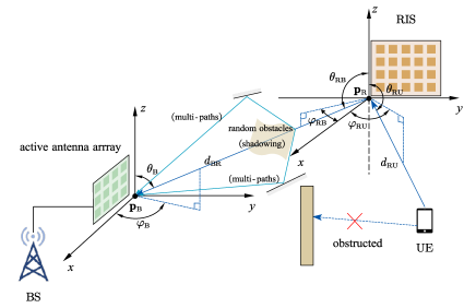
Figure 1: The geometry of the considered 3D RIS-assisted uplink localization scenario.

For the case adopting the exactly spherical wavefront model, by combining (2), it can be derived that [27]

$$d_{r\mathrm{U}}=\|\mathbf{p}_{\mathrm{U}}-\mathbf{p}_{r}\|=\sqrt{\rho_{\mathrm{R},r}^{2}+d_{\mathrm{RU}}^{2}+2d_{\mathrm{RU}}\Gamma_{r\mathrm{U}}},$$ (3)

where $\rho_{\mathrm{R},r}=\|\mathbf{p}_{\mathrm{R},r}\|$ denotes the distance between the $r$-th element and the reference point of the RIS; $\Gamma_{r\mathrm{U}}$ is given by

$$\Gamma_{r\mathrm{U}} =-x_{\mathrm{R},r}\sin\theta_{\mathrm{RU}}\cos\varphi_{\mathrm{RU}}-y_{\mathrm{R},r}\sin\theta_{\mathrm{RU}}\sin\varphi_{\mathrm{RU}}-z_{\mathrm{R},r}\cos\theta_{\mathrm{RU}},$$ (4)

For the traditional far-field case that the planar wavefront model is adopted, eq. (3) is expanded to the first order term as [36]

$$d_{r\mathrm{U}}\simeq d_{\mathrm{RU}}+\Gamma_{r\mathrm{U}}.$$ (5)

The matrix $\mathbf{\Upsilon}_{\mathrm{RU},n}=\mathrm{diag}\{\boldsymbol{\gamma}_{\mathrm{RU},n}\}$ reflects the different amplitudes across the RIS in the near-field scenario. The $r$-th element of $\boldsymbol{\gamma}_{\mathrm{RU},n}\in\mathbb{R}^{N_{\mathrm{R}}\times 1}$ is $[\boldsymbol{\gamma}_{\mathrm{RU},n}]_{r}=\frac{\sqrt{2P_{\mathrm{t}}}\lambda_{n}}{4\pi d_{r\mathrm{U}}}$. Note that in the far-field scenario, $\mathbf{\Upsilon}_{\mathrm{RU},n}\to\frac{\sqrt{2P_{\mathrm{t}}}\lambda_{n}}{4\pi d_{\mathrm{RU}}}\mathbf{I}$.

The matrix $\mathbf{H}_{\mathrm{BR},n}\in\mathbb{C}^{N_{\mathrm{B}}\times N_{\mathrm{R}}}$ in (1) represents the channel phase response between the BS and the RIS, which is expressed as $\mathbf{H}_{\mathrm{BR},n}=\mathbf{H}_{\mathrm{BR},n}^{\left(\mathrm{d}\right)}+\mathbf{H}_{\mathrm{BR},n}^{\left(\mathrm{multi}\right)}$. The matrix $\mathbf{H}_{\mathrm{BR},n}^{\left(\mathrm{d}\right)}$ represents the channel with respect to the LOS path between the BS and the RIS. Here we also consider both the near-field spherical wavefront and the far-field planar wavefront in this part of the channel. Then the $(b,r)$-th entry of $\mathbf{H}^{\left(\mathrm{d}\right)}_{\mathrm{BR},n}$ in both cases can be expressed as

$$[\mathbf{H}^{\left(\mathrm{d}\right)}_{\mathrm{BR},n}]_{b,r} =\frac{\lambda_{n}}{4\pi d_{br}}e^{-j2\pi f_{n}d_{br}/c}$$ (near-field) (6)

$$\simeq\frac{\lambda_{n}}{4\pi d_{\mathrm{BR}}}e^{-j2\pi f_{n}d_{br}/c}e^{-j2\pi f_{n}d_{\mathrm{BR}}/c}\left[\mathbf{a}_{\mathrm{B}}\mathbf{a}_{\mathrm{RB}}^{\top}\right]_{b,r}\;$$ (far-field) (7)

where $d_{br}$ denotes the distance between the $b$-th antenna at the BS and the $r$-th element of the RIS; $d_{\mathrm{BR}}=\|\mathbf{p}_{\mathrm{B}}-\mathbf{p}_{\mathrm{R}}\|$; $\mathbf{a}_{\mathrm{B}}\in\mathbb{C}^{N_{\mathrm{B}}\times 1}$ and $\mathbf{a}_{\mathrm{RB}}\in\mathbb{C}^{N_{\mathrm{R}}\times 1}$ are the far-field array steering vectors at the BS and the RIS, respectively. The $b$-th element of $\mathbf{a}_{\mathrm{B}}$ and the $r$-th element of $\mathbf{a}_{\mathrm{RB}}$ are given by

$$[\mathbf{a}_{\mathrm{B}}]_{b}=e^{-j2\pi f_{n}\Gamma_{\mathrm{B},b}},\quad[\mathbf{a}_{\mathrm{RB}}]_{r}=e^{-j2\pi f_{n}\Gamma_{r\mathrm{B}}},$$ (8)

where

$$\Gamma_{\mathrm{B},b} ={-}x_{\mathrm{B},b}\sin\theta_{\mathrm{B}}\cos\varphi_{\mathrm{B}}{-}y_{\mathrm{B},b}\sin\theta_{\mathrm{B}}\sin\varphi_{\mathrm{B}}{-}z_{\mathrm{B},b}\cos\theta_{\mathrm{B}},$$

$$\Gamma_{r\mathrm{B}} =-x_{\mathrm{R},r}\sin\theta_{\mathrm{RB}}\cos\varphi_{\mathrm{RB}}-y_{\mathrm{R},r}\sin\theta_{\mathrm{RB}}\sin\varphi_{\mathrm{RB}}-z_{\mathrm{R},r}\cos\theta_{\mathrm{RB}}.$$ (9)

Similar to the definition of $\mathbf{p}_{\mathrm{R},r}$, $\mathbf{p}_{\mathrm{B},b}\triangleq[x_{\mathrm{B},b},y_{\mathrm{B},b},z_{\mathrm{B},b}]^{\top}$ indicates the $b$-th antenna coordinate of the BS. The parameters $(\theta_{\mathrm{RB}},\varphi_{\mathrm{RB}})$ and $(\theta_{\mathrm{B}},\varphi_{\mathrm{B}})$ are the the elevation and azimuth angles of departure at the RIS and the angles of arrival at the BS, respectively. It is noteworthy that although this part of the channel does not directly contain the information of the UE position, adopting whether the near-field spherical wavefront model or the far-field planar wavefront model will still significantly affect the CRLB performance in localization, which will be discussed in Section IV-B and verified in Section V. The matrix $\mathbf{H}_{\mathrm{BR},n}^{\left(\mathrm{multi}\right)}$ represents channel respect to the multi-paths between the BS and the RIS. We adopt the independent, identically distributed (i.i.d.) Rayleigh fading model to characterize this part of the channel. Under this assumption, the entries of $\mathbf{H}_{\mathrm{BR},n}^{\left(\mathrm{multi}\right)}$ are i.i.d. circular symmetric complex Gaussian with variance $\sigma_{\mathrm{H}}^{2}$ [36].

The term $x_{n,t}{\sum_{i}{\beta_{i}\mathbf{h}_{\mathrm{BU},n}^{\left(i\right)}}}$ in (1) represents the signal received from the multi-paths, where $\beta_{i}$ and $\mathbf{h}_{\mathrm{BU},n}^{\left(i\right)}$ are the power attenuation and the channel phase response of the $i$-th path, respectively. This term has no contribution to the localization of the UE since the positions of the reflectors are not known. In other words, this part of the channel is uncontrollable. Usually, these uncontrollable multi-paths reflected from other scatterers are ignored, thanks to the strong path degradation in mmWave propagation [22]. For the case that the energy of the multi-paths cannot be ignored, one can adopt the signal components separation method introduced in [23] and [24] to extract the RIS-reflected component by exploiting the time dimension. Therefore, to focus on the role that the RIS plays in the localization, in the following analysis, we only consider the received signal from the path reflected by the RIS. Thus the received signal in (1) can be rewritten as

$$\mathbf{y}_{n,t} =\alpha x_{n,t}e^{-j2\pi f_{n}\xi}\mathbf{H}_{\mathrm{BR},n}\mathbf{\Phi}_{t}\mathbf{\Upsilon}_{\mathrm{RU},n}\mathring{\mathbf{h}}_{\mathrm{RU},n}+\mathbf{w}_{n,t},$$ (10)

$$=\boldsymbol{\mu}_{n,t}+\tilde{\mathbf{w}}_{\mathrm{n},\mathrm{t}}$$ (11)

where

$$\boldsymbol{\mu}_{n,t}\triangleq\alpha x_{n,t}e^{-j2\pi f_{n}\xi}\mathbf{H}_{\mathrm{BR},n}^{(\mathrm{d})}\mathbf{\Phi}_{t}\mathbf{\Upsilon}_{\mathrm{RU},n}\mathring{\mathbf{h}}_{\mathrm{RU},n},\quad\tilde{\mathbf{w}}_{\mathrm{n},\mathrm{t}}\triangleq\mathbf{H}_{\mathrm{BR},n}^{(\mathrm{multi})}\tilde{\mathbf{x}}_{n,t}+\mathbf{w}_{n,t}$$ (12)

with $\tilde{\mathbf{x}}_{n,t}=\alpha x_{n,t}e^{-j2\pi f_{n}\xi}\mathbf{\Phi}_{t}\mathbf{\Upsilon}_{\mathrm{RU},n}\mathring{\mathbf{h}}_{\mathrm{RU},n}$. The covariance matrix of the equivalent noise $\tilde{\mathbf{w}}_{\mathrm{n},\mathrm{t}}$ is then given by

$$\mathbf{C}_{\tilde{\mathbf{w}}_{n,t}}=\left(\left\|\tilde{\mathbf{x}}_{n,t}\right\|^{2}\sigma_{\mathrm{H}}^{2}+\sigma^{2}\right)\mathbf{I}=(\alpha^{2}|x_{n,t}|^{2}\left\|\boldsymbol{\gamma}_{\mathrm{RU},n}\right\|^{2}\sigma_{\mathrm{H}}^{2}+\sigma^{2})\mathbf{I}.$$ (13)

III The Fundamental Limits

In this section, based on the signal model (10), we derive the FIM and the CRLB for not only the unknown UE position but also the intermediate parameters that are related to the position information. The EFI results for the intermediate parameters will enable the further analysis in the following section. This section focuses on the near-field scenario between the RIS and the UE. The EFI for the far-field scenario will be investigated and compared with that for the near-field scenario in Section IV-A.

III-A The Position Error Bound

According to the localization scenario and the signal model introduced in Section II, the unknown parameter vector that contains the UE position and the other nuisance parameters is given by $\mathbf{\Theta}=\left[\alpha,c\xi,\mathbf{p}^{\top}_{\mathrm{U}}\right]^{\top}\in\mathbb{R}^{5\times 1}$. Suppose that the BS receives the signal in $T$ time slots. From (12), we note that both the signal part $\boldsymbol{\mu}_{n,t}$ and the equivalent noise part $\tilde{\mathbf{w}}_{\mathrm{n},\mathrm{t}}$ are related to $\mathbf{\Theta}$. Therefore, the FIM for $\mathbf{\Theta}$ is calculated as [27], [37]

$$\color[rgb]{0,0,1}\boldsymbol{\mathcal{J}}=\mathbf{J}_{\tilde{\mathbf{w}}}+\mathbf{J}_{\boldsymbol{\mu}}=\mathbf{J}_{\tilde{\mathbf{w}}}+\sum_{t=1}^{T}{\sum_{n=1}^{N}{\sum_{b=1}^{N_{\mathrm{B}}}{\mathbf{J}_{b,n,t}}}},$$ (14)

where $\mathbf{J}_{b,n,t}$ represents the Fisher information for $\mathbf{\Theta}$ provided by the signal part received via the $n$-th sub-carrier at the $b$-th antenna during the time slot $t$, i.e., a single sample, and it is given by

$$\mathbf{J}_{b,n,t}=\frac{2}{\sigma^{2}}\Re\left\{\frac{\partial\mu_{b,n,t}^{*}}{\partial\mathbf{\Theta}}\frac{\partial\mu_{b,n,t}}{\partial\mathbf{\Theta}^{\top}}\right\}\in\mathbb{R}^{5\times 5}$$ (15)

where

$$\color[rgb]{0,0,1}\mu_{b,n,t}\triangleq\left[\boldsymbol{\mu}_{n,t}\right]_{b}=\alpha x_{n,t}e^{-j2\pi f_{n}\xi}\mathbf{h}_{b\mathrm{R},n}^{\top}\mathbf{\Phi}_{t}\mathbf{\Upsilon}_{\mathrm{RU},n}\mathring{\mathbf{h}}_{\mathrm{RU},n}=\alpha x_{n,t}e^{-j2\pi f_{n}\xi}\boldsymbol{\phi}_{t}^{\top}\tilde{\mathbf{h}}_{b,n}$$ (16)

with $\mathbf{h}_{b\mathrm{R},n}\triangleq([\mathbf{H}_{\mathrm{BR},n}^{\left(\mathrm{d}\right)}]_{b,:})^{\top}$ and

$$\color[rgb]{0,0,1}\mathbf{\tilde{h}}_{b,n}\triangleq\mathbf{h}_{b\mathrm{R},n}\circledast\boldsymbol{\gamma}_{\mathrm{RU},n}\circledast\mathring{\mathbf{h}}_{\mathrm{RU},n}.$$ (17)

Note that the contribution of the inter-sample information for the parameters has been inherently included in $\mathbf{J}_{\boldsymbol{\mu}}$. Define $\mathbf{d}_{\mathrm{RU}}\triangleq\left[d_{1\mathrm{U}},...,d_{N_{\mathrm{R}}\mathrm{U}}\right]^{\top}$; $\dot{\mathbf{h}}_{b,n}\triangleq\mathbf{h}_{b\mathrm{R},n}\circledast\mathring{\mathbf{h}}_{\mathrm{RU},n}\circledast\dot{\mathbf{d}}_{\mathrm{RU}}$ where $[\dot{\mathbf{d}}_{\mathrm{RU}}]_{r}=-\frac{1}{d_{r\mathrm{U}}^{2}},(1\leq r\leq N_{\mathrm{R}})$;

$$\mathbf{D}_{\mathring{\mathbf{h}}\mathbf{p}}\triangleq\frac{\partial\mathring{\mathbf{h}}_{\mathrm{RU},n}}{\partial\mathbf{p}_{\mathrm{U}}^{\top}}=\frac{-j2\pi f_{n}}{c}\mathrm{diag}\left\{\tilde{\mathbf{h}}_{b,n}\right\}\frac{\partial\mathbf{d}_{\mathrm{RU}}}{\partial\mathbf{p}_{\mathrm{U}}^{\top}};$$ (18a)

$$\mathbf{D}_{\boldsymbol{\gamma}\mathbf{p}}\triangleq\frac{\partial\boldsymbol{\gamma}_{\mathrm{RU},n}}{\partial\mathbf{p}_{\mathrm{U}}^{\top}}=\frac{\sqrt{2P_{\mathrm{t}}}\lambda_{n}}{4\pi}\mathrm{diag}\left\{\dot{\mathbf{h}}_{b,n}\right\}\frac{\partial\mathbf{d}_{\mathrm{RU}}}{\partial\mathbf{p}_{\mathrm{U}}^{\top}};$$ (18b)

$\mathbf{D}_{\mathbf{hp}}\triangleq\mathbf{D}_{\mathring{\mathbf{h}}\mathbf{p}}+\mathbf{D}_{\boldsymbol{\gamma}\mathbf{p}}$. Note that $\mathbf{J}_{b,n,t}$ is symmetric and

$$\Re\left\{\frac{\partial\mu_{b,n,t}^{*}}{\partial\alpha}\frac{\partial\mu_{b,n,t}}{\partial\left(c\xi\right)}\right\}=\Re\left\{\frac{-j2\pi f_{n}\alpha|x_{n}|^{2}}{c}|\boldsymbol{\phi}_{t}^{\top}\mathbf{\tilde{h}}_{b,n}|^{2}\right\}=0,$$ (19)

Combining (15)–(19), $\mathbf{J}_{b,n,t}$ can be calculated as:

$$\mathbf{J}_{b,n,t}=\left[\begin{matrix}J_{\alpha\alpha}^{(b,n,t)}&0&(\mathbf{j}_{\alpha\mathbf{p}}^{(b,n,t)})^{\top}\\ 0&J_{\xi\xi}^{(b,n,t)}&(\mathbf{j}_{\xi\mathbf{p}}^{(b,n,t)})^{\top}\\ \mathbf{j}_{\alpha\mathbf{p}}^{(b,n,t)}&\mathbf{j}_{\xi\mathbf{p}}^{(b,n,t)}&\mathbf{J}_{\mathbf{pp}}^{(b,n,t)}\\ \end{matrix}\right],$$ (20)

where $\mathbf{j}_{\alpha\mathbf{p}}^{(b,n,t)},\mathbf{j}_{\xi\mathbf{p}}^{(b,n,t)}\in\mathbb{R}^{3\times 1}$, $\mathbf{J}_{\mathbf{pp}}\in\mathbb{R}^{3\times 3}$,

$$J_{\alpha\alpha}^{(b,n,t)} =\frac{2}{\sigma^{2}}|x_{n,t}|^{2}|\boldsymbol{\phi}_{t}^{\top}\mathbf{\tilde{h}}_{b,n}|^{2}, J_{\xi\xi}^{(b,n,t)} =\frac{8\pi^{2}f_{n}^{2}\alpha^{2}}{c^{2}\sigma^{2}}\left|x_{n,t}\right|^{2}|\boldsymbol{\phi}_{t}^{\top}\mathbf{\tilde{h}}_{b,n}|^{2},$$

$$\mathbf{j}_{\alpha\mathbf{p}}^{(b,n,t)} =\Re\biggl{\{}\frac{2\alpha|x_{n,t}|^{2}}{\sigma^{2}}\tilde{\mathbf{h}}_{b,n}^{\mathrm{H}}\boldsymbol{\phi}_{t}^{*}\boldsymbol{\phi}_{t}^{\top}\mathbf{D}_{\mathbf{hp}}\biggr{\}}^{\top},\, \mathbf{j}_{\xi\mathbf{p}}^{(b,n,t)} =\Re\biggl{\{}\frac{j4\pi f_{n}\alpha^{2}|x_{n,t}|^{2}}{c\sigma^{2}}\tilde{\mathbf{h}}_{b,n}^{\mathrm{H}}\boldsymbol{\phi}_{t}^{*}\boldsymbol{\phi}_{t}^{\top}\mathbf{D}_{\mathbf{hp}}\biggr{\}}^{\top},$$

$$\mathbf{J}_{\mathbf{pp}}^{(b,n,t)} =\Re\biggl{\{}\frac{2\alpha^{2}|x_{n,t}|^{2}}{\sigma^{2}}\mathbf{D}_{\mathbf{hp}}^{\mathrm{H}}\boldsymbol{\phi}_{t}^{*}\boldsymbol{\phi}_{t}^{\top}\mathbf{D}_{\mathbf{hp}}\biggr{\}}.$$ (21)

Note that $d_{r\mathrm{U}}$ is a direct function of $\mathbf{p}_{\mathrm{U}}$ when adopting the exactly spherical wavefront model, then the $r$-th row of the Jacobian matrix $\frac{\partial\mathbf{d}_{\mathrm{RU}}}{\partial\mathbf{p}_{\mathrm{U}}^{\top}}\in\mathbb{R}^{N_{\mathrm{R}}\times 3}$ in (18) in the near-field scenario (combining (3)) is given by

$$\left[\frac{\partial\mathbf{d}_{\mathrm{RU}}}{\partial\mathbf{p}_{\mathrm{U}}^{\top}}\right]_{r,:}=\frac{\partial\|\mathbf{p}_{\mathrm{U}}-\mathbf{p}_{r}\|}{\partial\mathbf{p}_{\mathrm{U}}^{\top}}=\frac{\left(\mathbf{p}_{\mathrm{U}}-\mathbf{p}_{r}\right)^{\top}}{d_{r\mathrm{U}}}.$$ (22)

The matrix $\mathbf{J}_{\tilde{\mathbf{w}}}$ represents the Fisher information provided by the equivalent noise part. The $(i,j)$-th entry of $\mathbf{J}_{\tilde{\mathbf{w}}}$ ($1\leq i,j\leq 5$) is expressed as [37]

$$[\mathbf{J}_{\tilde{\mathbf{w}}}]_{i,j}=\sum_{t=1}^{T}{\sum_{n=1}^{N}{\mathrm{tr}\left\{\mathbf{C}_{\tilde{\mathbf{w}}_{n,t}}^{-1}\frac{\partial\mathbf{C}_{\tilde{\mathbf{w}}_{n,t}}}{\partial\left[\mathbf{\Theta}\right]_{i}}\mathbf{C}_{\tilde{\mathbf{w}}_{n,t}}^{-1}\frac{\partial\mathbf{C}_{\tilde{\mathbf{w}}_{n,t}}}{\partial\left[\mathbf{\Theta}\right]_{j}}\right\}}}.$$ (23)

Combining (13), we have $\frac{\partial\mathbf{C}_{\tilde{\mathbf{w}}_{n,t}}}{\partial\left(c\xi\right)}=\mathbf{0}$,

$$\frac{\partial\mathbf{C}_{\tilde{\mathbf{w}}_{n,t}}}{\partial\alpha} =2\alpha|x_{n,t}|^{2}\left\|\boldsymbol{\gamma}_{\mathrm{RU},n}\right\|^{2}\sigma_{\mathrm{H}}^{2}\mathbf{I}\triangleq{c}_{\alpha\left(n,t\right)}\sigma_{\mathrm{H}}^{2}\mathbf{I},$$ (24)

$$\frac{\partial\mathbf{C}_{\tilde{\mathbf{w}}_{n,t}}}{\partial\left[\mathbf{p}_{\mathrm{U}}\right]_{k}} =2\alpha^{2}\frac{\sqrt{2P_{\mathrm{t}}}\lambda_{n}}{4\pi}\left|x_{n,t}\right|^{2}\boldsymbol{\gamma}_{\mathrm{RU},n}^{\mathrm{T}}\left(\dot{\mathbf{d}}_{\mathrm{RU}}\circledast\frac{\partial\mathbf{d}_{\mathrm{RU}}}{\partial\left[\mathbf{p}_{\mathrm{U}}\right]_{k}}\right)\sigma_{\mathrm{H}}^{2}\mathbf{I}\triangleq\left[{\mathbf{c}}_{\mathbf{p}\left(n,t\right)}\right]_{k}\sigma_{\mathrm{H}}^{2}\mathbf{I}.$$ (25)

where $1\leq k\leq 3$, $\frac{\partial\mathbf{d}_{\mathrm{RU}}}{\partial[\mathbf{p}_{\mathrm{U}}]_{k}}=\bigl{[}\frac{\partial\mathbf{d}_{\mathrm{RU}}}{\partial\mathbf{p}_{\mathrm{U}}^{\top}}\bigr{]}_{:,k}$. Define ${\mathbf{c}}_{\mathbf{\Theta}\left(n,t\right)}=[{c}_{\alpha\left(n,t\right)},0,{\mathbf{c}}^{\top}_{\mathbf{p}\left(n,t\right)}]^{\top}$, $\mathbf{J}_{\tilde{\mathbf{w}}}$ can be further calculated as

$$\mathbf{J}_{\tilde{\mathbf{w}}}=\sum_{t=1}^{T}{\sum_{n=1}^{N}{\frac{N_{\mathrm{B}}\sigma_{\mathrm{H}}^{4}}{\left(\alpha^{2}|x_{n,t}|^{2}\left\|\boldsymbol{\gamma}_{\mathrm{RU},n}\right\|^{2}\sigma_{\mathrm{H}}^{2}+\sigma^{2}\right)^{2}}}}{\mathbf{c}}_{\mathbf{\Theta}\left(n,t\right)}{\mathbf{c}}_{\mathbf{\Theta}\left(n,t\right)}^{\top}.$$ (26)

Finally, the PEB is defined as [27], [29]

$$\mathrm{PEB}(\boldsymbol{\mathcal{J}})=\sqrt{\mathrm{tr}([\boldsymbol{\mathcal{J}}^{-1}]_{3:5,3:5})}.$$ (27)

Remark 1

Since

$$\color[rgb]{0,0,1}\mathbf{J}_{\boldsymbol{\mu}}-\mathbf{J}^{\prime}_{\boldsymbol{\mu}}\triangleq\mathbf{J}_{\boldsymbol{\mu}}-\sum_{t,t\neq t^{\prime}}{\sum_{n,n\neq n^{\prime}}{\sum_{b,b\neq b^{\prime}}{\mathbf{J}_{b,n,t}}}}=\mathbf{J}_{b^{\prime},n^{\prime},t^{\prime}}\succeq\mathbf{0},$$ (28)

it can be verified that the CRLBs corresponding to $\mathbf{J}_{\boldsymbol{\mu}}$ and $\mathbf{J}^{\prime}_{\boldsymbol{\mu}}$ satisfy $\mathbf{J}_{\boldsymbol{\mu}}^{-1}\preceq(\mathbf{J}^{\prime}_{\boldsymbol{\mu}})^{-1}$ [38, Corollary 7.7.4]. In other words, adding a sample (with Fisher information $\mathbf{J}_{b^{\prime},n^{\prime},t^{\prime}}$) will generally improve the localization performance [37]. Similarly, the information carried by the multi-paths between the BS and the RIS, which corresponds to $\mathbf{J}_{\tilde{\mathbf{w}}}$, is also able to help improve the estimation performance. Besides, we note that according to (14), $\mathbf{J}_{\boldsymbol{\mu}}$ intrinsically contains the information about $\mathbf{\Theta}$ provided by all the samples, and we can trade one of the space, bandwidth or time resource for the other two while maintaining the same CRLB performance, which will be shown in Section V.

III-B EFI For the Intermediate Parameters

In order to give more insights in the analysis of how the localization performance is influenced by the system configuration, we introduce the intermediate parameters, including the unknown distance and direction of the UE observed at the RIS, which is related to the UE position. The corresponding parameter vector is then defined as $\mathbf{\bar{\Theta}}=\left[\alpha,c\xi,d_{\mathrm{RU}},\varphi_{\mathrm{RU}},\theta_{\mathrm{RU}}\right]^{\top}\in\mathbb{R}^{5\times 1}$. The FIM of $\mathbf{\bar{\Theta}}$ is given by $\bar{\boldsymbol{\mathcal{J}}}=\bar{\mathbf{J}}_{\tilde{\mathbf{w}}}+\bar{\mathbf{J}}_{\boldsymbol{\mu}}=\bar{\mathbf{J}}_{\tilde{\mathbf{w}}}+\sum_{t=1}^{T}{\sum_{n=1}^{N}{\sum_{b=1}^{N_{\mathrm{B}}}{\bar{\mathbf{J}}_{b,n,t}}}}.$ First we derive $\bar{\mathbf{J}}_{b,n,t}$. Define $\boldsymbol{\eta}=\left[d_{\mathrm{RU}},\varphi_{\mathrm{RU}},\theta_{\mathrm{RU}}\right]^{\top}$,

$$\tilde{\mathbf{d}}_{\boldsymbol{\eta}_{k}}\triangleq\tilde{\mathbf{h}}_{b,n}\circledast\frac{\partial\mathbf{d}_{\mathrm{RU}}}{\partial[\boldsymbol{\eta}]_{k}},\quad\dot{\mathbf{d}}_{\boldsymbol{\eta}_{k}}\triangleq\dot{\mathbf{h}}_{b,n}\circledast\frac{\partial\mathbf{d}_{\mathrm{RU}}}{\partial[\boldsymbol{\eta}]_{k}}.$$ (29)

where $1\leq k\leq 3$. Combining (3) and (4), in the near-field scenario the $r$-th element of $\frac{\partial\mathbf{d}_{\mathrm{RU}}}{\partial[\boldsymbol{\eta}]_{k}}\in\mathbb{R}^{N_{\mathrm{R}}\times 1}$ can be calculated as

$$\left[\frac{\partial\mathbf{d}_{\mathrm{RU}}}{\partial[\boldsymbol{\eta}]_{1}}\right]_{r}=\frac{\partial{d}_{r\mathrm{U}}}{\partial d_{\mathrm{RU}}}=\frac{1}{d_{r\mathrm{U}}}\left(d_{\mathrm{RU}}+\Gamma_{r\mathrm{U}}\right),$$ (30a)

$$\left[\frac{\partial\mathbf{d}_{\mathrm{RU}}}{\partial[\boldsymbol{\eta}]_{2}}\right]_{r}=\frac{\partial{d}_{r\mathrm{U}}}{\partial\varphi_{\mathrm{RU}}}=\frac{d_{\mathrm{RU}}}{d_{r\mathrm{U}}}(x_{\mathrm{R},r}\sin\theta_{\mathrm{RU}}\sin\varphi_{\mathrm{RU}}-y_{\mathrm{R},r}\sin\theta_{\mathrm{RU}}\cos\varphi_{\mathrm{RU}}),$$ (30b)

$$\left[\frac{\partial\mathbf{d}_{\mathrm{RU}}}{\partial[\boldsymbol{\eta}]_{3}}\right]_{r}=\frac{\partial{d}_{r\mathrm{U}}}{\partial\theta_{\mathrm{RU}}}=\frac{d_{\mathrm{RU}}}{d_{r\mathrm{U}}}(-x_{\mathrm{R},r}\cos\theta_{\mathrm{RU}}\cos\varphi_{\mathrm{RU}}-y_{\mathrm{R},r}\cos\theta_{\mathrm{RU}}\sin\varphi_{\mathrm{RU}}+z_{\mathrm{R},r}\sin\theta_{\mathrm{RU}}),$$ (30c)

where $1\leq r\leq N_{\mathrm{R}}$. Then $\mathbf{\bar{J}}_{b,n,t}$ can be expressed as

$$\bar{\mathbf{J}}_{b,n,t}=\left[\begin{matrix}J_{\alpha\alpha}^{(b,n,t)}&0&(\mathbf{j}_{\alpha\boldsymbol{\eta}}^{(b,n,t)})^{\top}\\ 0&J_{\xi\xi}^{(b,n,t)}&(\mathbf{j}_{\xi\boldsymbol{\eta}}^{(b,n,t)})^{\top}\\ \mathbf{j}_{\alpha\boldsymbol{\eta}}^{(b,n,t)}&\mathbf{j}_{\xi\boldsymbol{\eta}}^{(b,n,t)}&\mathbf{J}_{\boldsymbol{\eta\eta}}^{(b,n,t)}\\ \end{matrix}\right],$$ (31)

where $J_{\alpha\alpha}^{(b,n,t)}$ and $J_{\xi\xi}^{(b,n,t)}$ are defined in (III-A),

$$[\mathbf{j}_{\alpha\boldsymbol{\eta}}^{(b,n,t)}]_{k} =\Re\biggl{\{}\frac{2\alpha|x_{n,t}|^{2}}{\sigma^{2}}\tilde{\mathbf{h}}_{b,n}^{\mathrm{H}}\boldsymbol{\phi}_{t}^{*}\boldsymbol{\phi}_{t}^{\top}\left(\frac{-j2\pi f_{n}}{c}\tilde{\mathbf{d}}_{\boldsymbol{\eta}_{k}}+\frac{\sqrt{2P_{\mathrm{t}}}\lambda_{n}}{4\pi}\dot{\mathbf{d}}_{\boldsymbol{\eta}_{k}}\right)\biggr{\}},$$

$$[\mathbf{j}_{\xi\boldsymbol{\eta}}^{(b,n,t)}]_{k} =\Re\biggl{\{}\frac{j4\pi f_{n}\alpha^{2}|x_{n,t}|^{2}}{c\sigma^{2}}\tilde{\mathbf{h}}_{b,n}^{\mathrm{H}}\boldsymbol{\phi}_{t}^{*}\boldsymbol{\phi}_{t}^{\top}\left(\frac{-j2\pi f_{n}}{c}\tilde{\mathbf{d}}_{\boldsymbol{\eta}_{k}}+\frac{\sqrt{2P_{\mathrm{t}}}\lambda_{n}}{4\pi}\dot{\mathbf{d}}_{\boldsymbol{\eta}_{k}}\right)\biggr{\}},$$

$$\left[\mathbf{J}_{\boldsymbol{\eta\eta}}^{(b,n,t)}\right]_{k,l} =\Re\biggl{\{}\frac{8\pi^{2}\alpha^{2}f_{n}^{2}|x_{n,t}|^{2}}{c^{2}\sigma^{2}}\tilde{\mathbf{d}}_{\boldsymbol{\eta}_{k}}^{\mathrm{H}}\boldsymbol{\phi}_{t}^{*}\boldsymbol{\phi}_{t}^{\top}\tilde{\mathbf{d}}_{\boldsymbol{\eta}_{l}}\biggr{\}}+\Re\left\{\frac{\alpha^{2}P_{\mathrm{t}}\lambda_{n}^{2}|x_{n,t}|^{2}}{4\pi^{2}\sigma^{2}}\dot{\mathbf{d}}_{\boldsymbol{\eta}_{k}}^{\mathrm{H}}\boldsymbol{\phi}_{t}^{*}\boldsymbol{\phi}_{t}^{\top}\dot{\mathbf{d}}_{\boldsymbol{\eta}_{l}}\right\}$$

$$\mathrel{\phantom{=}}+\Re\left\{\frac{j2\sqrt{2P_{\mathrm{t}}}\alpha^{2}|x_{n,t}|^{2}}{\sigma^{2}}\tilde{\mathbf{d}}_{\boldsymbol{\eta}_{k}}^{\mathrm{H}}\boldsymbol{\phi}_{t}^{*}\boldsymbol{\phi}_{t}^{\top}\dot{\mathbf{d}}_{\boldsymbol{\eta}_{l}}\right\},$$ (32)

where $1\leq k,l\leq 3$.

Then we derive $\bar{\mathbf{J}}_{\tilde{\mathbf{w}}}$. Define ${\mathbf{c}}_{\bar{\mathbf{\Theta}}\left(n,t\right)}=[{c}_{\alpha\left(n,t\right)},0,{\mathbf{c}}^{\top}_{\boldsymbol{\eta}\left(n,t\right)}]^{\top}$, where ${c}_{\alpha\left(n,t\right)}$ is given in (24). Combining (30), the $k$-th element of ${\mathbf{c}}_{\boldsymbol{\eta}\left(n,t\right)}$ is defined as

$$\frac{\partial\mathbf{C}_{\tilde{\mathbf{w}}_{n,t}}}{\partial\left[\boldsymbol{\eta}\right]_{k}}=2\alpha^{2}\frac{\sqrt{2P_{\mathrm{t}}}\lambda_{n}}{4\pi}\left|x_{n,t}\right|^{2}\boldsymbol{\gamma}_{\mathrm{RU},n}^{\mathrm{T}}\left(\dot{\mathbf{d}}_{\mathrm{RU}}\circledast\frac{\partial\mathbf{d}_{\mathrm{RU}}}{\partial\left[\boldsymbol{\eta}\right]_{k}}\right)\sigma_{\mathrm{H}}^{2}\mathbf{I}\triangleq\left[{\mathbf{c}}_{\boldsymbol{\eta}\left(n,t\right)}\right]_{k}\sigma_{\mathrm{H}}^{2}\mathbf{I}.$$ (33)

Therefore, $\bar{\mathbf{J}}_{\tilde{\mathbf{w}}}$ is given by

$$\bar{\mathbf{J}}_{\tilde{\mathbf{w}}}=\sum_{t=1}^{T}{\sum_{n=1}^{N}{\frac{N_{\mathrm{B}}\sigma_{\mathrm{H}}^{4}}{\left(\alpha^{2}|x_{n,t}|^{2}\left\|\boldsymbol{\gamma}_{\mathrm{RU},n}\right\|^{2}\sigma_{\mathrm{H}}^{2}+\sigma^{2}\right)^{2}}}}{\mathbf{c}}_{\bar{\mathbf{\Theta}}\left(n,t\right)}{\mathbf{c}}_{\bar{\mathbf{\Theta}}\left(n,t\right)}^{\top}.$$ (34)

Unlike the traditional analysis that the CRLBs for the intermediate parameters $d_{\mathrm{RU}}$, $\varphi_{\mathrm{RU}}$ and $\theta_{\mathrm{RU}}$ are obtained by extracting the corresponding diagonal element of $\bar{\boldsymbol{\mathcal{J}}}^{-1}$, we adopt the notion of EFI to evaluate the estimation performance limits of the intermediate parameters [14]. First define

$$\bar{E}(k)\triangleq[{\color[rgb]{0,0,1}\bar{\boldsymbol{\mathcal{J}}}}]_{k,k}-[{\color[rgb]{0,0,1}\bar{\boldsymbol{\mathcal{J}}}}]_{k,\left(1:5\right)\setminus k}[{\color[rgb]{0,0,1}\bar{\boldsymbol{\mathcal{J}}}}]_{\left(1:5\right)\setminus k,\left(1:5\right)\setminus k}^{-1}[{\color[rgb]{0,0,1}\bar{\boldsymbol{\mathcal{J}}}}]_{\left(1:5\right)\setminus k,k},$$ (35)

where $k\in\{3,4,5\}$. The index set $(1:5)\backslash k$ contains all the indexes from $1$ to $5$ except index $k$. Then the EFI for $d_{\mathrm{RU}}$, $\varphi_{\mathrm{RU}}$ and $\theta_{\mathrm{RU}}$ are given by [14]

$$\bar{J}_{\mathrm{E}}(d_{\mathrm{RU}})=\bar{E}(3)=\frac{1}{[{{\color[rgb]{0,0,1}\bar{\boldsymbol{\mathcal{J}}}}}^{-1}]_{3,3}};\quad\bar{J}_{\mathrm{E}}(\varphi_{\mathrm{RU}})=\bar{E}(4)=\frac{1}{[{{\color[rgb]{0,0,1}\bar{\boldsymbol{\mathcal{J}}}}}^{-1}]_{4,4}};\quad\bar{J}_{\mathrm{E}}(\theta_{\mathrm{RU}})=\bar{E}(5)=\frac{1}{[{{\color[rgb]{0,0,1}\bar{\boldsymbol{\mathcal{J}}}}}^{-1}]_{5,5}}.$$ (36)

Note that the EFI given in (36) quantifies the information limits about the intermediate parameters that could be attained from the received samples.

IV The Impact of Each Part of the Cascaded Channel on the Fundamental Limits

In this section, we analyze how the three parts of the cascaded channel, namely $\mathbf{h}_{\mathrm{RU},n}$, $\mathbf{H}_{\mathrm{BR},n}$ and $\mathbf{\Phi}_{t}$, influence the fundamental limits of the near-field localization. Based on the analysis and the results in Section III, we investigate the near-field effect in both RIS-UE and BS-RIS part of the channel, and compare the results with those of the far-field scenario. Besides, we also reveal that the well-known focusing control scheme for the RIS may degrade the localization performance in the asynchronous scenario.

IV-A Near-field vs. Far-field: RIS-UE Part

First we focus on the channel between the UE and the RIS. In this part of the channel, when the spherical wavefront is considered as (3), (22) and (30), both the FIM ${\boldsymbol{\mathcal{J}}}$ and $\bar{\boldsymbol{\mathcal{J}}}$ are generally invertible and the EFI for the intermediate parameters (36) are positive with adequate samples, which means that theoretically the position of the UE and all the intermediate parameters related to the position can be estimated in the near-field scenario. That is, although the TOA information cannot be inferred due to the synchronization mismatch $\xi$ and the unknown attenuation $\alpha$, the position information of the UE can be obtained from the curvature of the spherical wavefront passively sensed by the RIS. However, as the distance between the user and the RIS $d_{\mathrm{RU}}\to\infty$ or when the far-field planar wavefront is adopted as (5), we will prove that it is impossible to localize the UE because the position-related parameter $d_{\mathrm{RU}}$ cannot be estimated.

Proposition 1

When $d_{\mathrm{RU}}\to\infty$ or the far-field scenario is considered in the RIS-UE part of the channel, the EFI for the distance parameter $\bar{J}_{\mathrm{E}}(d_{\mathrm{RU}})=0$, regardless of whether considering the multi-paths between the BS and the RIS.

Proof:

Please refer to Appendix A. ∎

When $d_{\mathrm{RU}}\to\infty$, the wavefront tends to be planar as the far-field scenario. According to Proposition 1, in this case we are unable to obtain any information about the distance parameter $d_{\mathrm{RU}}$ with the existence of the synchronization mismatch $\xi$. Because in the near-field scenario, the values of $\frac{\partial{d}_{r\mathrm{U}}}{\partial d_{\mathrm{RU}}}$ are different across different $r$, the RIS is able to collect the information about $d_{\mathrm{RU}}$ from the spherical wavefront through the phase differences and the amplitude differences caused by $d_{\mathrm{RU}}$ at different RIS elements. However, when the wavefront tends to be planar, from (A.1) $\frac{\partial{d}_{r\mathrm{U}}}{\partial d_{\mathrm{RU}}}\to 1$ for all $r$, which means that in the far-field scenario the RIS cannot collect the information about the parameter $d_{\mathrm{RU}}$ since no phase difference or amplitude difference caused by $d_{\mathrm{RU}}$ exists.

It is worth underlining that the direction of the UE can still be estimated when the wavefront tends to be planar. In the far field scenario, $\mu_{b,n,t}$ can be expressed as

$$\color[rgb]{0,0,1}\mu_{b,n,t}\simeq\alpha x_{n,t}e^{-j2\pi f_{n}(c\xi+d_{\mathrm{RU}})/c}\gamma_{\mathrm{RU},n}\boldsymbol{\phi}_{t}^{\top}(\mathbf{h}_{b\mathrm{R},n}\circledast\hat{\mathbf{h}}_{\mathrm{RU},n}),$$ (37)

where $[\hat{\mathbf{h}}_{\mathrm{RU},n}]_{r}=e^{-j2\pi f_{n}\Gamma_{r\mathrm{U}}/c}$ for $1\leq r\leq N_{\mathrm{R}}$. It can be drawn (as in Section V) that, when investigating the following parameter $\bar{\mathbf{\Theta}}^{\prime}=\left[\alpha,c\xi+d_{\mathrm{RU}},\varphi_{\mathrm{RU}},\theta_{\mathrm{RU}}\right]^{\top}\in\mathbb{R}^{4\times 1}$, the EFI for the direction related parameters $\varphi_{\mathrm{RU}}$ and $\theta_{\mathrm{RU}}$ are generally positive in both near-field and far-field scenarios. When $d_{\mathrm{RU}}\to\infty$ or the planar wavefront is considered, $\frac{\partial{d}_{r\mathrm{U}}}{\partial\varphi_{\mathrm{RU}}}$ and $\frac{\partial{d}_{r\mathrm{U}}}{\partial\theta_{\mathrm{RU}}}$ are still different for different $r$ as:

$$\frac{\partial{d}_{r\mathrm{U}}}{\partial\varphi_{\mathrm{RU}}} \to x_{\mathrm{R},r}\sin\theta_{\mathrm{RU}}\sin\varphi_{\mathrm{RU}}-y_{\mathrm{R},r}\sin\theta_{\mathrm{RU}}\cos\varphi_{\mathrm{RU}},$$

$$\frac{\partial{d}_{r\mathrm{U}}}{\partial\theta_{\mathrm{RU}}} \to-x_{\mathrm{R},r}\cos\theta_{\mathrm{RU}}\cos\varphi_{\mathrm{RU}}-y_{\mathrm{R},r}\cos\theta_{\mathrm{RU}}\sin\varphi_{\mathrm{RU}}+z_{\mathrm{R},r}\sin\theta_{\mathrm{RU}}.$$ (38)

Therefore, unlike the distance parameter $d_{\mathrm{RU}}$, the phase differences caused by $\varphi_{\mathrm{RU}}$ and $\theta_{\mathrm{RU}}$ exist at different RIS elements in both near-field and far-field scenarios.

IV-B Near-field vs. Far-field: BS-RIS Part

IV-B1 Spatial Gain vs. Power Gain

Unlike the traditional localization scenario that the BS, equipped with an active large-scale antenna array, directly receives the signal transmitted from the UE, there is an extra part of the channel $\mathbf{H}_{\mathrm{BR},n}$ between the BS and the RIS cascaded with $\mathbf{h}_{\mathrm{RU},n}$ in the RIS-assisted localization scenario. In this subsection, we investigate the impact of the BS-RIS part of the channel on the localization CRLB in both near-field and far-field scenarios. This part of the channel is assumed to be determined since both the BS position and the RIS position are known in advance. The information of the UE position is not directly contained in this part of the channel. However, in the following discussions, we will reveal that this part of the channel determines the type of the gain provided by the BS antenna array.

Let $\mathbf{J}^{(\mathrm{B})}_{\boldsymbol{\mu}b}=\sum_{t=1}^{T}{\sum_{n=1}^{N}}\mathbf{J}_{b,n,t}$ denote the Fisher information provided by all time slots and sub-carriers at antenna $b$, then we have $\mathbf{J}_{\boldsymbol{\mu}}=\sum_{b=1}^{N_{\mathrm{B}}}\mathbf{J}^{(\mathrm{B})}_{\boldsymbol{\mu}b}$. According to the discussion in Remark 1, we know that $\mathbf{J}_{\boldsymbol{\mu}}\succeq\mathbf{J}^{(\mathrm{B})}_{\boldsymbol{\mu}b}$, thus $\mathrm{PEB}(\mathbf{J}_{\boldsymbol{\mu}})\leq\mathrm{PEB}(\mathbf{J}^{(\mathrm{B})}_{\boldsymbol{\mu}b})$ for any $b$, which indicates that the multiple antennas at the BS can improve the CRLB performance. In the near-field scenario as (6), $\mathbf{J}^{(\mathrm{B})}_{\boldsymbol{\mu}b}$ is generally different for different $b$, that is, each antenna at the BS can provide independent spatial gain for the FIM. While in the far-field scenario, we will show in Proposition 2 that the multiple antennas at the BS only provide the power gain for the FIM. That is, in this case the PEB decreases linearly with $\sqrt{N_{\mathrm{B}}}$, regardless of whether considering the multi-paths between the BS and the RIS.

Proposition 2

When the far-field scenario is considered as (7) for $\mathbf{H}_{\mathrm{BR},n}^{\mathrm{(d)}}$, $\mathbf{J}^{(\mathrm{B})}_{\boldsymbol{\mu}b}$ is identical for all $b$, and $\mathrm{PEB}(\boldsymbol{\mathcal{J}})\propto\frac{1}{\sqrt{N_{\mathrm{B}}}}$.

Proof:

Please refer to Appendix B. ∎

IV-B2 Case Investigation

To vividly show the different impacts of the two types of the gain on the CRLB performance, we then investigate the following case. Suppose that only a single carrier with index $n_{0}$ is used and the signal lasts only a single time slot $t_{0}$, during which the reflection coefficients of the RIS are unchanged. In this case $\mathbf{J}^{(\mathrm{B})}_{\boldsymbol{\mu}b}=\mathbf{J}_{b,n_{0},t_{0}}$, which makes $\mathbf{J}^{(\mathrm{B})}_{\boldsymbol{\mu}b}$ a singular matrix with rank $2$ [26]. Besides, in this case

$$\mathbf{J}_{\tilde{\mathbf{w}}}=\frac{\sigma_{\mathrm{H}}^{4}}{\left(\alpha^{2}|x_{n_{0},t_{0}}|^{2}\left\|\boldsymbol{\gamma}_{\mathrm{RU},n}\right\|^{2}\sigma_{\mathrm{H}}^{2}+\sigma^{2}\right)^{2}}{\mathbf{c}}_{\mathbf{\Theta}\left(n_{0},t_{0}\right)}{\mathbf{c}}_{\mathbf{\Theta}\left(n_{0},t_{0}\right)}^{\top}$$ (39)

which has rank 1. Thus $\boldsymbol{\mathcal{J}}$ is also singular, which means that it is impossible to localize the UE through a single antenna under these circumstances. Moreover, when the far-field scenario is considered for $\mathbf{H}_{\mathrm{BR,n_{0}}}^{(\mathrm{d})}$, $\mathbf{J}_{\boldsymbol{\mu}}=N_{\mathrm{B}}\mathbf{J}^{(\mathrm{B})}_{\boldsymbol{\mu}b}$ is also a rank 2 singular matrix. In other words, even if we collect the information from all antennas, we are still unable to localize the UE because in this scenario the gain provided by the antenna array at the BS for the localization is power gain, which can not increase the rank of the FIM. However, in the near-field scenario for $\mathbf{H}_{\mathrm{BR,n_{0}}}^{(\mathrm{d})}$, the FIM $\mathbf{J}_{\boldsymbol{\mu}}=\sum_{b=1}^{N_{\mathrm{B}}}\mathbf{J}^{(\mathrm{B})}_{\boldsymbol{\mu}b}$ will generally become a full rank invertible matrix with adequate antennas. In this scenario, the gain provided by the antenna array at the BS for the localization is defined as spatial gain, which can increase the rank of the FIM. Therefore, unlike the far-field scenario, in this case we are theoretically possible to localize the UE.

We can understand the above results from another perspective of view. Note that $\mathbf{H}_{\mathrm{BR},n_{0}}^{(\mathrm{d})}$ is irrelevant to $\mathbf{\Theta}$, then the Jacobian matrix $\frac{\partial\boldsymbol{\mu}_{n_{0},t_{0}}}{\partial\mathbf{\Theta}^{\top}}\in\mathbb{C}^{N_{\mathrm{B}}\times 5}$ can be expressed as

$$\color[rgb]{0,0,1}\frac{\partial\boldsymbol{\mu}_{n_{0},t_{0}}}{\partial\mathbf{\Theta}^{\top}}=\mathbf{H}_{\mathrm{BR},n_{0}}^{(\mathrm{d})}\frac{\partial\alpha x_{n,t}e^{-j2\pi f_{n}\xi}\mathbf{\Phi}_{t_{0}}\mathbf{\Upsilon}_{\mathrm{RU},n_{0}}\mathring{\mathbf{h}}_{\mathrm{RU},n_{0}}}{\partial\mathbf{\Theta}^{\top}}.$$ (40)

In this case, $\mathbf{J}_{\boldsymbol{\mu}}$ can be rewritten as

$$\mathbf{J}_{\boldsymbol{\mu}}=\frac{2}{\sigma^{2}}\Re\left\{\frac{\partial\boldsymbol{\mu}_{n_{0},t_{0}}^{\mathrm{H}}}{\partial\mathbf{\Theta}}\frac{\partial\boldsymbol{\mu}_{n_{0},t_{0}}}{\partial\mathbf{\Theta}^{\top}}\right\}.$$ (41)

In the far-field scenario, obviously $\frac{\partial\boldsymbol{\mu}_{n_{0},t_{0}}}{\partial\mathbf{\Theta}^{\top}}$ has rank $1$ since $\mathbf{H}_{\mathrm{BR},n_{0}}^{(\mathrm{d})}$ has rank $1$, according to (7). Therefore, from (41), again we find that $\mathbf{J}_{\boldsymbol{\mu}}$ is a singular matrix with rank $2$, while in the near-field scenario, $\mathbf{H}_{\mathrm{BR},n_{0}}^{(\mathrm{d})}$ has full rank $N_{\mathrm{B}}$ (assuming $N_{\mathrm{B}}<N_{\mathrm{R}}$). Therefore, with large enough $N_{\mathrm{B}}$, $\frac{\partial\boldsymbol{\mu}_{n_{0},t_{0}}}{\partial\mathbf{\Theta}^{\top}}$ will also generally become a full rank matrix with rank $5$, which eventually makes $\mathbf{J}_{\boldsymbol{\mu}}$ and the FIM $\boldsymbol{\mathcal{J}}$ invertible. From this case, we find that the rank of the BS-RIS part of the channel matrix $\mathbf{H}_{\mathrm{BR},n_{0}}^{(\mathrm{d})}$ plays an important role.

Proposition 3

In the single-carrier, single snapshot case, it requires both the BS-RIS part and the RIS-UE part of the channel work in the near-field scenario to localize the UE. The near-field effect in the RIS-UE part of the channel makes the RIS could passively sense the UE position through COA information, while the near-field effect in the BS-RIS part of the channel makes the multiple BS antennas provide sufficient degrees of freedom to extract the COA information.

Remark 2

In this case where the information received by a single antenna is insufficient to estimate $\boldsymbol{\Theta}$, the power gain in the far-field scenario does not improve the CRLB performance, while the spatial gain does. Indeed, for the same system parameters, when there is no much information about $\mathbf{\Theta}$ (provided by all the time slots and sub-carriers) at each single antenna, the spatial gain usually achieves a better CRLB performance than the power gain. However, when adequate information about $\mathbf{\Theta}$ can be obtained from a single BS antenna, the power gain may outperform the spatial gain, which will be shown in Section V. Besides, in the practical situation when the positions of the BS and the RIS are fixed, we can determine the gain type we prefer achieving by adjusting the antenna separation at the BS. We can reduce the antenna separation if we prefer achieving the power gain, while we can increase the antenna separation if the effect of the spatial gain is preferred.

IV-C The Impact of the RIS Coefficients

The reflection coefficient profile of the RIS, namely $\boldsymbol{\phi}_{t}$, is another important parameter that can significantly influence the CRLB performance. The random phase profile has been adopted and evaluated in many existing works [26]–[29] since it is simple to implement. However, as pointed out in these works, the random phase profile usually cannot perform as well as the dedicated phase profile which is designed according to certain criterion. The focusing control plan, which takes maximizing the received SNR as the design criterion, has been investigated not only in the traditional wireless communications as a pre-coding scheme [34] but also in the RIS-assisted localization [27]–[29] as a RIS control scheme. This efficient scheme avoids tackling the complex high-dimensional non-convex problem of directly optimizing the RIS configuration for the minimum PEB. The optimal SNR will lead to optimal spectral efficiency, which usually means better communication performance [26]. In the localization scenario investigated in this paper, however, the optimal SNR (or in other words the maximum RIS gain) does not ensure the optimal CRLB performance. In fact, in some cases, we could barely obtain any information about the UE’s position can be obtained when the maximum received SNR is achieved with focusing scheme.

Denote $\bar{{\mathbf{J}}}_{\mathrm{E}}(\boldsymbol{\eta})$ as the EFIM for the position related intermediate parameters $\boldsymbol{\eta}$, given by

$$\color[rgb]{0,0,1}\bar{{\mathbf{J}}}_{\mathrm{E}}(\boldsymbol{\eta})=[\bar{\boldsymbol{\mathcal{J}}}]_{3:5,3:5}-[\bar{\boldsymbol{\mathcal{J}}}]_{3:5,1:2}[\bar{\boldsymbol{\mathcal{J}}}]_{1:2,1:2}^{-1}[\bar{\boldsymbol{\mathcal{J}}}]_{1:2,3:5}.$$ (42)

Let $\mathbf{h}_{b\mathrm{R},n}=\boldsymbol{\gamma}_{b\mathrm{R},n}\circledast\mathring{\mathbf{h}}_{b\mathrm{R},n}$, where $[\boldsymbol{\gamma}_{b\mathrm{R},n}]_{r}=\frac{\lambda_{n}}{4\pi d_{br}}$, $[\mathring{\mathbf{h}}_{b\mathrm{R},n}]_{r}=e^{-j2\pi f_{n}d_{br}/c}$ ($1\leq r\leq N_{\mathrm{R}}$).

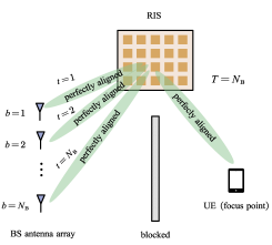
(a)

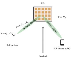
(b)

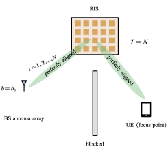
(c)

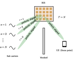
(d)

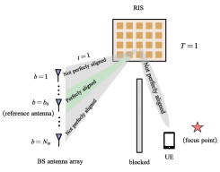
(e)

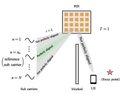
(f)

Figure 2: Schematic diagrams of Case 1, Case2, and the more practical situation. (a) Case1, SD. (b) Case1, FD. (c) Case2, SD. (d) Case2, FD. (e) Practical situation, SD. (f) Practical situation, FD. SD: Spatial domain. FD: Frequency domain.

Proposition 4

When the multi-paths effect can be ignored between the BS and the RIS, in the following two cases $\mathbf{\bar{J}}_{\mathrm{E}}(\boldsymbol{\eta})\approx\mathbf{0}$.

Case 1: Only a single carrier with index $n_{0}$ is used and $N_{\mathrm{B}}$ time slots are employed, and the size of the BS antenna array $L_{\mathrm{B}}\ll d_{\mathrm{BR}}$. The time varying phase profiles of the RIS are set as $\boldsymbol{\phi}_{t_{1}}=(\mathring{\mathbf{h}}_{t_{1}\mathrm{R},n_{0}}\circledast\mathring{\mathbf{h}}_{\mathrm{RU},n_{0}})^{*}$. Only the antenna with index $t_{1}$ is activated and the received signal is sampled during time slot $t_{1}$.

Case 2: Only a single antenna with index $b_{0}$ is used and $N$ time slots are employed, and the bandwidth of the signal $f_{N}-f_{c}\ll f_{c}$. The time varying phase profiles of the RIS are set as $\boldsymbol{\phi}_{t_{2}}=(\mathring{\mathbf{h}}_{b_{0}\mathrm{R},t_{2}}\circledast\mathring{\mathbf{h}}_{\mathrm{RU},t_{2}})^{*}$ for $1\leq t_{2}\leq N$. Only the received signal at sub-carrier $t_{2}$ is sampled during time slot $t_{2}$.

Proof:

Please refer to Appendix C. ∎

The schematic diagrams of Case1 and Case 2 in both spatial domain and frequency domain are shown in Figs. 2(a)-(d). In Case 1, the RIS with coefficient $\boldsymbol{\phi}_{t_{1}}$ focuses the signal from the focus point $\mathbf{p}_{\mathrm{U}}$ to different antennas at different time slots. Therefore, all $N_{\mathrm{B}}$ antennas receive the signal with the maximum SNR in this case. The situation in Case 2 is similar, the SNR of the received signal at each sub-carrier is maximized. However, the EFIM $\mathbf{\bar{J}}_{\mathrm{E}}(\boldsymbol{\eta})\approx\mathbf{0}$ in the two cases, which means that we can barely obtain any information about the direction and the distance of the UE, that is, the position of the UE cannot be effectively estimated. The maximum received SNR, which usually means optimal communication performance, but leads to the worst localization performance in the two cases. The intuitive understanding of this result is that, when the unknown synchronization mismatch and the shadowing effect attenuation exist, the position information of the UE is provided only by the spherical wavefront sensed by the RIS. Therefore, estimating the position related parameters (namely $d_{\mathrm{RU}}$, $\varphi_{\mathrm{RU}}$ and $\theta_{\mathrm{RU}}$) all relies on the phase differences and the amplitude differences at different RIS elements caused by these parameters. The focusing scheme, which achieves the maximum SNR (or equivalently the maximum RIS gain) by aligning the received signal at all RIS elements when observed either at each BS antenna in Case 1 or at each sub-carrier in Case 2, makes the phase differences vanish. The remaining amplitude differences information is not sufficient to effectively locate the UE because the amplitude differences across an array are far less significant compared with the phase differences. Thus the position related parameters cannot be effectively estimated in these circumstances.

Remark 3

In practical situations, we can get the signal from all antennas and sub-carries in a single time slot and usually the UE does not locate exactly at the focusing point (as shown in Figs. 2(e)-(f)), which makes the EFIM $\mathbf{\bar{J}}_{\mathrm{E}}(\boldsymbol{\eta})\succ\mathbf{0}$. However, what we want to reveal in Proposition 4 is that the localization performance could be degraded with the increase of the received SNR, as will be verified in Section V. In other words, maximizing the RIS gain, which ensures better communication performance, is not always a good objective for the asynchronous RIS-assisted localization. Besides, as will be shown in Section V, this conclusion still holds when the multi-paths between the BS and the RIS cannot be ignored. Further study is required on investigating how to efficiently set the RIS configuration to achieve an optimal localization performance in this scenario. Some insights are provided in Section V-C.

V Numerical Results

This section presents the numerical results to evaluate the performance limits of the RIS-assisted localization and the intermediate-parameter estimation. Besides, the properties revealed in Section IV are verified in this section. The 3D localization scenario is depicted in Fig. 1. Unless indicated otherwise, some basic system parameters are set as follows. The carrier frequency is set as $f_{c}=28$ GHz. The reference points of the RIS and the BS are assumed to be located at $\mathbf{p}_{\mathrm{R}}=[0,0,0]^{\top}$(m) and $\mathbf{p}_{\mathrm{B}}=[8,-12,2]^{\top}$(m), respectively. Both the RIS and the antenna array at the BS are lying on the Y-Z plane. The RIS is assumed to be a passive URA with $N_{\mathrm{R}}=60\times 60=3600$ elements and the BS is equipped with an active URA with $N_{\mathrm{B}}=8\times 8=64$ antennas. The spacing of two adjacent RIS elements is set as $\Delta r={\lambda_{c}}/{2}$ where $\lambda_{c}$ is the carrier wavelength. The multi-paths between the BS and the RIS are considered in this section, the corresponding Rician factor $\kappa$ is set as $5\,$dB.

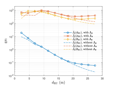
Figure 3: The EFI of intermediate parameters as a function of the distance between the RIS and the UE. The received signal power is fixed.

V-A RIS-UE Part Near-Field Effect on PEB

In this subsection, we focus on the near-field effect in the RIS-UE part of the channel. The power of the received signal from different locations is fixed in order to highlight the effect of the spherical wavefront. The random phase profile is adopted at the RIS, the bandwidth of the transmitted signal is set as $400$ MHz, and a single time slot is considered.

Fig. 3 shows the EFI of the position-related intermediate parameters as a function of $d_{\mathrm{RU}}$ with and without considering the multi-paths between the BS and the RIS. From Fig. 3, with the increase of the distance between the RIS and the UE, the EFI of the distance parameter $d_{\mathrm{RU}}$ tends to $0$ regardless of whether considering the multi-paths between the BS and the RIS, which is exactly the reason of the poor PEB when the UE is far from the RIS as discussed in Section IV-A. However, the EFI of the direction-related parameters $\theta_{\mathrm{RU}}$ and $\phi_{\mathrm{RU}}$ remains high regardless of $d_{\mathrm{RU}}$, which also verifies that the direction of arrival with high-accuracy is attainable in both scenarios. Besides, the EFI for all the position related parameters are generally improved when the multi-paths between the BS and the RIS are considered, which verifies the discussion in Remark 1.

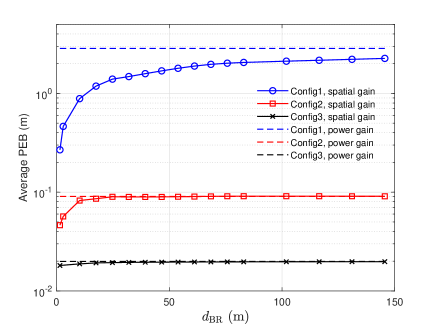
(a)

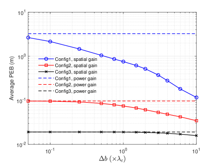
(b)

Figure 4: Average PEB of 100 Mont Carlo trials with random RIS coefficients vs. $d_{\mathrm{BR}}$ and the BS antenna separation $\Delta b$. The UE is located in $\mathbf{p}_{\mathrm{U}}=[4,2.1,-1]^{\top}$, the received signal power is fixed at each point.

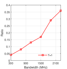
(a)

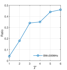
(b)

Figure 5: The ratio that the power gain outperforms the spatial gain within 100 Mont Carlo trials with random RIS coefficients. BW: bandwidth.

V-B Comparisons between the Spatial Gain and the Power Gain

In this subsection, we focus on the BS-RIS part of the channel and compare the effect of the two different kinds of performance gains introduced in Section IV-B on PEB. 100 Mont Carlo trials with random RIS coefficients are carried out under different system configurations.

TABLE I: A Notation of the System Configurations

Configuration	Bandwidth	Time slots
Config1	300MHz	$T=1$
Config2	2500MHz	$T=1$
Config3	2500MHz	$T=3$

In Fig. 4a, the received signal power is fixed and the spacing of two adjacent BS antennas is set as $\Delta b=\lambda_{c}/2$. The average PEBs of 100 Mont Carlo trials are depicted as a function of the distance between the BS and the RIS. Three system configurations are evaluated as listed in Table I. As expected, the spatial gain will approach the power gain as $d_{\mathrm{BR}}$ increases under all system configurations because the near-field model (6) will approach the far-field model (7) when $d_{\mathrm{BR}}\to\infty$. Besides, from the perspective of view of the average PEB, the spatial gain significantly outperforms the power gain when there is no much time and bandwidth resource at a single antenna (Config1). However, in Config2 and Config3, the performance gap tends to be negligible with the increase of bandwidth and time slots. Similar phenomena can be observed from Fig. 4b. The only difference is that, in Fig. 4b, without adjusting $d_{\mathrm{BR}}$, we could still let the spatial gain tend to approach the power gain by decreasing $\Delta b$, as discussed in Remark 2. In addition, from Fig. 4b, a small increase of the antenna separation $\Delta{b}$ could result in significant spatial gain when the time and bandwidth resources are deficient as Config1, whereas a tremendous increase of $\Delta{b}$ is required to achieve observable spatial gain with abundant space and time resource as Config3.

To further demonstrate the impact of the bandwidth and time resources on the two different types of gains, Fig. 5 depicts the ratio that the power gain outperforms the spatial gain within 100 Mont Carlo trials. From Fig. 5, the probability that the power gain is with better performance increases as the increase of bandwidth and time slots, which further verifies the discussion in Remark 2. This is because the spatial gain can be deemed as providing new degrees of freedom, while the power gain simply ‘amplify’ the information linearly. When the time and bandwidth resources are deficient, there is no much information about the position of the UE at a single antenna. Therefore, obtaining more degrees of freedom is certainly more effective than simply linearly ‘amplifying’ such information. However, with the increase of time and bandwidth resources, the information of the UE position that we are able to collect from a single antenna becomes sufficient to accurately localize the UE. In this situation, ‘amplifying’ such abundant information becomes profitable, while the influence of providing more degrees of freedom becomes limited.

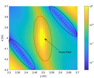
(a)

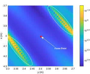
(b)

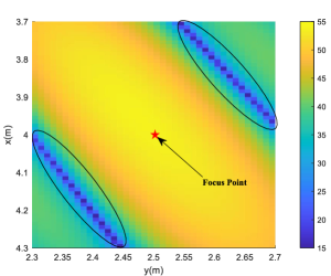
(c)

Figure 6: The PEB and the received SNR at $z=-1$ plane with focusing control scheme at the RIS. (a) The PEB of asynchronous scenario. Bandwidth $=40$MHz. (b) The PEB of synchronous scenario. (c) The received SNR.

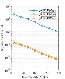
(a)

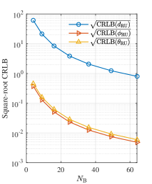
(b)

Figure 7: The square-root CRLBs of the intermediate parameters at the focus point as a function of bandwidth and $N_{\mathrm{B}}$ in the asynchronous scenario. (a) $N_{\mathrm{B}}=4$ is fixed. (b) Bandwidth $=10$ MHz is fixed.

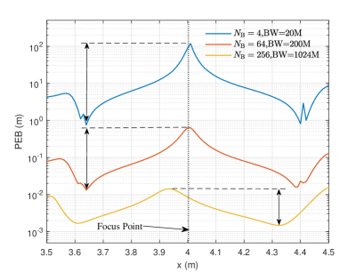
Figure 8: The PEBs along $x$ axis with focusing control scheme under different system configurations. $y=2.5$ and $z=-1$ are fixed.

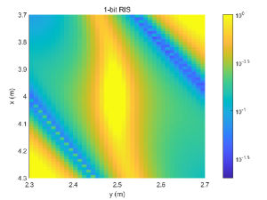
(a)

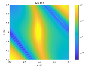
(b)

(c)

Figure 9: The PEB at $z=-1$ plane when adopting focusing control scheme with discrete RIS coefficients.

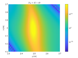
(a)

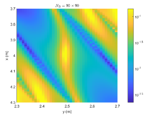
(b)

Figure 10: The PEB at $z=-1$ plane when adopting focusing control scheme with different RIS sizes.

V-C Evaluation of the Focusing Control Scheme

In this subsection, the PEB performances are evaluated when the focusing control plan is adopted for the RIS in both synchronous and asynchronous scenarios. The RIS is set to focus the signal with frequency 28 GHz (carrier frequency) from position $(4,2.5,-1)$ to the reference point of the BS antenna array in a single time slot. We get the samples of the received signal from all the antennas and sub-carriers in this time slot.

Figs. 6(a) and 6(b) depict the PEBs at $z=-1$ plane with focusing scheme in asynchronous and synchronous scenarios, respectively. The corresponding received SNR of this region is depicted in Fig. 6(c). The bandwidth of the transmitted signal is set as $40$ MHz. From Fig. 6(a), a ‘peak’ of the PEB occurs around the focus point (as circled by the red ellipse), which indicates a worse localization performance in this region. However, the region around the focus point is with the highest SNR as confirmed in Fig. 6(c). Besides, Comparing the regions circled by the black ellipses in Figs. 6(a) and (c), the received SNRs of the two regions are relatively much lower than the area around the focus point, but the PEB performances are much better. The above results also indicate that, if we intend to minimize the PEB at a specific position $\mathbf{p}_{0}$, a good choice for RIS coefficients that may achieve a decent PEB performance is to try focusing the signal near $\mathbf{p}_{0}$, instead of precisely at this position. Based on this observation, we are able to efficiently obtain a good initial point for further optimizing the RIS coefficients. Note that although in this subsection, the received signals are not perfectly aligned at most of the antennas and sub-carriers as shown in Figs. 2(e) and (f), and the EFIM for $\boldsymbol{\eta}$ is not $\mathbf{0}$ at the focus point (unlike the Case 1 and Case 2 in Proposition 4), the simulation results still verify that in the asynchronous scenario, the localization performance may be degraded with the increase of the received SNR, which is consistent with the discussion in Remark 3. Moreover, the simulation results also verify that the discussion in Section IV-C still holds in the scenario that the multi-paths between the BS and the RIS cannot be ignored. However, from Fig. 6(b), in the synchronous scenario, the ‘peak’ of the PEB around the focus point disappears and in general the PEB decreases with the increase of the received SNR, which is unlike the asynchronous scenario. That is because, firstly, in the synchronous scenario the TOA information is attainable, thus the distance parameter $d_{\mathrm{RU}}$ can be directly recovered from the TOA which does not rely on the phase differences at different RIS elements. Therefore, the higher SNR will generally lead to better distance estimation performance. Besides, in Fig. 7, the square-root CRLBs vs. the bandwidth and $N_{\mathrm{B}}$ at the focus point are depicted when adopting the focusing scheme. Although the direction of the UE still relies on the phase-differences at the RIS elements in the synchronous scenario, from Fig. 7, the high-accuracy direction related parameters (namely $\theta_{\mathrm{RU}}$ and $\phi_{\mathrm{RU}}$) can be obtained much more easily than the distance parameters when only relying on the phase differences caused by the wavefront. For example, note that $0.01$ rad (less than $0.6^{\circ}$) estimation error of $\theta_{\mathrm{RU}}$ and $\phi_{\mathrm{RU}}$ only leads to less than $0.1$ metre localization error when $d_{\mathrm{RU}}$ is less than $10$ metres (assuming $d_{\mathrm{RU}}$ is accurately estimated). However, from Fig. 7, when about $0.01$ rad root-square CRLBs of $\theta_{\mathrm{RU}}$ and $\phi_{\mathrm{RU}}$ are achieved, the square-root CRLB of $d_{\mathrm{RU}}$ is more than 1 metre, which means that the estimation error of $d_{\mathrm{RU}}$ is dominated in this scenario. In other words, obtaining high-accuracy distance parameter is the bottleneck of the near-field high-accuracy localization. Therefore, in the synchronous scenario where the higher SNR could lead to better $d_{\mathrm{RU}}$ estimation performance, in general the PEB will also be improved with the increase of SNR. Moreover, comparing Fig. 7(a) with Fig. 7(b), the estimation performance of the intermediate parameters can be improved by either increasing the spatial resource (namely $N_{\mathrm{B}}$) or the bandwidth resource, which is consistent with the discussion in Remark 1.

In Fig. 8, the PEBs along $x$ axis are depicted, and $y=2.5$ and $z=-1$ are fixed to evaluate the influence of different system configurations on the relative size of the ‘peak’ around the focus point. From Fig. 8, the ‘peak’ of the PEB will be alleviated when the number of the BS antennas and the bandwidth increase. That is because the signal reflected from the RIS will tend to be less aligned with the increase of antennas and bandwidth, which leads to more significant phase differences at the RIS from the focus point.

In Fig. 9, we investigate the impact of quantizing the phase of the RIS, which can reduce the complexity of the RIS. Comparing with Fig. 6(a), the differences on PEB are negligible when the 3-bit RIS is adopted. Besides, in Fig. 10, we evaluate the PEB performances for various RIS sizes. As expected, the RIS with a larger size could generally lead to a better PEB performance, and the ‘peak’ area around the focus point shrinks with the increase of the RIS elements. In other words, increase the size of the RIS will alleviate the PEB performance degradation effect around the focus point.

VI Conclusions

In this paper, the PEB of the RIS-based asynchronous localization and the EFI for the position-related intermediate parameters have been derived under the circumstances that the multi-paths between the BS and the RIS are considered. The more accurate model is adopted that takes the amplitude differences across the RIS and the BS into account. Based on the derived EFI, we first prove that in the asynchronous scenario, it is theoretically possible to localize the UE when the near-field spherical wavefront is considered in the RIS-UE part of the channel. However, with the increase of the distance from the UE to the RIS, the EFI for the distance parameter tends to $0$. We then revealed that when the near-field model was considered for the BS-RIS part of the channel, the multiple antennas at the BS can provide independent spatial gain, while only the power gain is provided by the antennas when this part of the channel works in the far-field scenario. The spatial gain outperforms the power gain when there is no much information about the UE position at each single antenna. But when there is adequate information at each antenna, the probability that the power gain achieves better PEB performance will increase. We also showed that the well-known focusing control scheme for the RIS, which maximizes the received SNR, is not always a good choice for localization, since it may reduce the phase differences caused by the spherical wavefront at the RIS and degrade the localization performance in the asynchronous scenario.

Appendix A

In this appendix we prove Proposition 1. When the far-field scenario is considered, according to (5) we have $\frac{\partial{d}_{r\mathrm{U}}}{\partial d_{\mathrm{RU}}}=1$ for all $r$. While in the near-field scenario, when we let $d_{\mathrm{RU}}\to\infty$, combining (3) and (30a) we also have

$$\lim_{d_{\mathrm{RU}}\to\infty}\frac{\partial{d}_{r\mathrm{U}}}{\partial d_{\mathrm{RU}}}=\lim_{d_{\mathrm{RU}}\to\infty}\frac{1}{d_{r\mathrm{U}}}\left(d_{\mathrm{RU}}+\Gamma_{r\mathrm{U}}\right)=1.$$ (A.1)

Therefore, in the above two cases one obtains $\frac{\partial\mathbf{d}_{\mathrm{RU}}}{\partial\left[\boldsymbol{\eta}\right]_{3}}=\frac{\partial\mathbf{d}_{\mathrm{RU}}}{\partial d_{\mathrm{RU}}}=\mathbf{1}_{N_{\mathrm{R}}}$ and $\boldsymbol{\gamma}_{\mathrm{RU},n}\to\frac{\sqrt{2P_{\mathrm{t}}}\lambda_{n}}{4\pi d_{\mathrm{RU}}}\mathbf{1}$. Under these circumstances we have

$$\frac{\sqrt{2P_{\mathrm{t}}}\lambda_{n}}{4\pi}\dot{\mathbf{h}}_{b,n}=-\frac{1}{d_{\mathrm{RU}}}\tilde{\mathbf{h}}_{b,n}.$$ (A.2)

Combining (A.2), each element of $\bar{\mathbf{J}}_{\boldsymbol{\mu}}$ can be further calculated as

$$[\bar{\mathbf{J}}_{\boldsymbol{\mu}}]_{1,1}=\sum_{t=1}^{T}{\sum_{n=1}^{N}{\sum_{b=1}^{N_{\mathrm{B}}}{\frac{2|x_{n,t}|^{2}}{\sigma^{2}}\left|\boldsymbol{\phi}_{t}^{\top}\tilde{\mathbf{h}}_{b,n}\right|^{2}}}},\quad[\bar{\mathbf{J}}_{\boldsymbol{\mu}}]_{1,2}=[\bar{\mathbf{J}}_{\boldsymbol{\mu}}]_{2,1}=0,$$ (A.3a)

$$[\bar{\mathbf{J}}_{\boldsymbol{\mu}}]_{1,3}=[\bar{\mathbf{J}}_{\boldsymbol{\mu}}]_{3,1}=\sum_{t=1}^{T}{\sum_{n=1}^{N}{\sum_{b=1}^{N_{\mathrm{B}}}{-\frac{2\alpha|x_{n,t}|^{2}}{d_{\mathrm{RU}}\sigma^{2}}\left|\boldsymbol{\phi}_{t}^{\top}\tilde{\mathbf{h}}_{b,n}\right|^{2}}}},$$ (A.3b)

$$[\bar{\mathbf{J}}_{\boldsymbol{\mu}}]_{1,k+2}=[\bar{\mathbf{J}}_{\boldsymbol{\mu}}]_{k+2,1}=\sum_{t=1}^{T}{\sum_{n=1}^{N}{\sum_{b=1}^{N_{\mathrm{B}}}{\Re\biggl{\{}\frac{-j4\pi f_{n}\alpha|x_{n}|^{2}}{c\sigma^{2}}\tilde{\mathbf{h}}_{b,n}^{\mathrm{H}}\boldsymbol{\phi}_{t}^{*}\boldsymbol{\phi}_{t}^{\top}\tilde{\mathbf{d}}_{\boldsymbol{\eta}_{k}}\biggr{\}}}}}$$ (A.3c)

$$[\bar{\mathbf{J}}_{\boldsymbol{\mu}}]_{2,2}=[\bar{\mathbf{J}}_{\boldsymbol{\mu}}]_{2,3}=[\bar{\mathbf{J}}_{\boldsymbol{\mu}}]_{3,2}=\sum_{t=1}^{T}{\sum_{n=1}^{N}{\sum_{b=1}^{N_{\mathrm{B}}}{\frac{8\pi^{2}\alpha^{2}f_{n}^{2}|x_{n}|^{2}}{c^{2}\sigma^{2}}\left|\boldsymbol{\phi}_{t}^{\top}\tilde{\mathbf{h}}_{b,n}\right|^{2}}}},$$ (A.3d)

$$[\bar{\mathbf{J}}_{\boldsymbol{\mu}}]_{2,k+2}=[\bar{\mathbf{J}}_{\boldsymbol{\mu}}]_{k+2,2}=\sum_{t=1}^{T}{\sum_{n=1}^{N}{\sum_{b=1}^{N_{\mathrm{B}}}{\Re\biggl{\{}\frac{8\pi^{2}\alpha^{2}f_{n}^{2}|x_{n}|^{2}}{c^{2}\sigma^{2}}\tilde{\mathbf{h}}_{b,n}^{\mathrm{H}}\boldsymbol{\phi}_{t}^{*}\boldsymbol{\phi}_{t}^{\top}\tilde{\mathbf{d}}_{\boldsymbol{\eta}_{k}}\biggr{\}}}}},$$ (A.3e)

$$[\bar{\mathbf{J}}_{\boldsymbol{\mu}}]_{3,3}=\sum_{t=1}^{T}{\sum_{n=1}^{N}{\sum_{b=1}^{N_{\mathrm{B}}}{\left(\frac{8\pi^{2}\alpha^{2}f_{n}^{2}|x_{n}|^{2}}{c^{2}\sigma^{2}}+\frac{2\alpha^{2}|x_{n}|^{2}}{d_{\mathrm{RU}}^{2}\sigma^{2}}\right)\left|\boldsymbol{\phi}_{t}^{\top}\tilde{\mathbf{h}}_{b,n}\right|^{2}}}},$$ (A.3f)

$$[\bar{\mathbf{J}}_{\boldsymbol{\mu}}]_{k+2,3}=[\bar{\mathbf{J}}_{\boldsymbol{\mu}}]_{3,k+2}=\sum_{t=1}^{T}{\sum_{n=1}^{N}{\sum_{b=1}^{N_{\mathrm{B}}}{\Re\biggl{\{}\left(\frac{8\pi^{2}\alpha^{2}f_{n}^{2}|x_{n}|^{2}}{c^{2}\sigma^{2}}+\frac{j4\pi f_{n}\alpha^{2}|x_{n}|^{2}}{d_{\mathrm{RU}}c\sigma^{2}}\right)\tilde{\mathbf{h}}_{b,n}^{\mathrm{H}}\boldsymbol{\phi}_{t}^{*}\boldsymbol{\phi}_{t}^{\top}\tilde{\mathbf{d}}_{\boldsymbol{\eta}_{k}}\biggr{\}}}}}.$$ (A.3g)

where $k\in\{2,3\}$. Besides, since in the far-field scenario $\left\|\boldsymbol{\gamma}_{\mathrm{RU},n}\right\|^{2}=N_{\mathrm{R}}\left(\frac{\sqrt{2P_{\mathrm{t}}}\lambda_{n}}{4\pi d_{\mathrm{RU}}}\right)^{2}\triangleq N_{\mathrm{R}}\gamma_{\mathrm{RU},n}^{2}$, we have

$$\frac{\partial\mathbf{C}_{\tilde{\mathbf{w}}_{n,t}}}{\partial\alpha}=2N_{\mathrm{R}}\alpha|x_{n,t}|^{2}N_{\mathrm{R}}\gamma_{\mathrm{RU},n}^{2}\sigma_{\mathrm{H}}^{2}\mathbf{I}\triangleq{c}_{\alpha\left(n,t\right)}\sigma_{\mathrm{H}}^{2}\mathbf{I},$$ (A.4a)

$$\frac{\partial\mathbf{C}_{\tilde{\mathbf{w}}_{n,t}}}{\partial d_{\mathrm{RU}}}=-\alpha^{2}|x_{n,t}|^{2}\gamma_{\mathrm{RU},n}\frac{\sqrt{2P_{\mathrm{t}}}\lambda_{n}}{2\pi d_{\mathrm{RU}}^{2}}\sigma_{\mathrm{H}}^{2}\mathbf{I}\triangleq c_{d\left(n,t\right)}\sigma_{\mathrm{H}}^{2}\mathbf{I},$$ (A.4b)

$$\frac{\partial\mathbf{C}_{\tilde{\mathbf{w}}_{n,t}}}{\partial\left(c\xi\right)}=\frac{\partial\mathbf{C}_{\tilde{\mathbf{w}}_{n,t}}}{\partial\varphi_{\mathrm{RU}}}=\frac{\partial\mathbf{C}_{\tilde{\mathbf{w}}_{n,t}}}{\partial\theta_{\mathrm{RU}}}=\mathbf{0}.$$ (A.4c)

Note that from (A.4),

$$c_{d\left(n,t\right)}=-\frac{\alpha}{d_{\mathrm{RU}}}c_{\alpha\left(n,t\right)},$$ (A.5)

$$[\bar{\mathbf{J}}_{\tilde{\mathbf{w}}_{n,t}}]_{:,2}=\left([\bar{\mathbf{J}}_{\tilde{\mathbf{w}}_{n,t}}]_{2,:}\right)^{\top}=\mathbf{0},\quad[\bar{\mathbf{J}}_{\tilde{\mathbf{w}}_{n,t}}]_{4:5,:}=\left([\bar{\mathbf{J}}_{\tilde{\mathbf{w}}_{n,t}}]_{:,4:5}\right)^{\top}=\mathbf{0}$$ (A.6)

Thus according to (A.3) and (A.4)-(A.5), it can be verified that

$$-\frac{\alpha}{d_{\mathrm{RU}}}[\bar{\mathbf{J}}_{\boldsymbol{\mu}}]_{\left(1:5\right)\setminus 3,1}+[\bar{\mathbf{J}}_{\boldsymbol{\mu}}]_{\left(1:5\right)\setminus 3,2}=[\bar{\mathbf{J}}_{\boldsymbol{\mu}}]_{\left(1:5\right)\setminus 3,3}$$ (A.7)

$$-\frac{\alpha}{d_{\mathrm{RU}}}[\bar{\mathbf{J}}_{\tilde{\mathbf{w}}_{n,t}}]_{1,1}=[\bar{\mathbf{J}}_{\tilde{\mathbf{w}}_{n,t}}]_{1,3},\quad-\frac{\alpha}{d_{\mathrm{RU}}}[\bar{\mathbf{J}}_{\tilde{\mathbf{w}}_{n,t}}]_{3,1}=[\bar{\mathbf{J}}_{\tilde{\mathbf{w}}_{n,t}}]_{3,3}$$ (A.8)

Therefore, combining (36) and (A.6)-(A.8), regardless of whether $\bar{\mathbf{J}}_{\tilde{\mathbf{w}}}=\mathbf{0}$, we have

$$\bar{J}_{\mathrm{E}}(d_{\mathrm{RU}}) =[\bar{\boldsymbol{\mathcal{J}}}]_{3,3}-[\bar{\boldsymbol{\mathcal{J}}}]_{3,\left(1:5\right)\setminus 3}\cdot\left[-\alpha/d_{\mathrm{RU}},1,0,0\right]^{\top}$$

$$=[\bar{\boldsymbol{\mathcal{J}}}]_{3,3}-(-\frac{\alpha}{d_{\mathrm{RU}}}[\bar{\boldsymbol{\mathcal{J}}}]_{3,1}+[\bar{\boldsymbol{\mathcal{J}}}]_{3,2})=0.$$ (A.9)

Thus complete the proof.

Appendix B

In this appendix we prove Proposition 2. We first rewrite $\mu_{b,n,t}$ in the far-field scenario as

$$\mu_{b,n,t} \color[rgb]{0,0,1}=\alpha x_{n}e^{-j2\pi f_{n}\xi}\sum_{r=1}^{N_{\mathrm{R}}}{\frac{\lambda_{n}}{4\pi d_{\mathrm{B}r}}\frac{\sqrt{2P_{\mathrm{t}}}\lambda_{n}}{4\pi d_{r\mathrm{U}}}e^{j\phi_{r,t}}e^{-j2\pi f_{n}\left(d{{}_{br}}+d_{r\mathrm{U}}\right)/c}}$$ (B.1)

$$\simeq e^{-j2\pi f_{n}\left(d_{\mathrm{BR}}+\Gamma_{\mathrm{B},b}\right)/c}\cdot F_{n,t},$$ (B.2)

where $\phi_{r,t}=[\boldsymbol{\phi}_{t}]_{r}$; $F_{n,t}$ is defined as

$$\color[rgb]{0,0,1}F_{n,t}\triangleq\alpha x_{n}e^{-j2\pi f_{n}\xi}\sum_{r=1}^{N_{\mathrm{R}}}{\frac{\lambda_{n}}{4\pi d_{\mathrm{B}r}}\frac{\sqrt{2P_{\mathrm{t}}}\lambda_{n}}{4\pi d_{r\mathrm{U}}}e^{j\phi_{r,t}}e^{-j2\pi f_{n}\left(\Gamma_{r\mathrm{B}}+d_{r\mathrm{U}}\right)/c}}.$$ (B.3)

Eq.(B.2) holds when the BS-RIS part of the channel works in the far-field scenario (by combining (7) and (8)). It is straightforward to verify that $\frac{\partial e^{-j2\pi f_{n}\left(d_{\mathrm{BR}}+\Gamma_{\mathrm{B},b}\right)/c}}{\partial\mathbf{\Theta}}=\mathbf{0}$. Therefore, in this case we have $\frac{\partial\mu_{b,n,t}}{\partial\mathbf{\Theta}^{\top}}=e^{-j2\pi f_{n}\left(d_{\mathrm{BR}}+\Gamma_{\mathrm{B},b}\right)/c}\frac{\partial F_{n,t}}{\partial\mathbf{\Theta}^{\top}}$, and each element of $\mathbf{J}^{(\mathrm{B})}_{\boldsymbol{\mu}b}$ is then given by

$$[\mathbf{J}^{(\mathrm{B})}_{\boldsymbol{\mu}b}]_{i,j}=\sum_{t=1}^{T}{\sum_{n=1}^{N}{\frac{2}{\sigma^{2}}\Re\left\{\frac{\partial\mu_{b,n,t}^{*}}{\partial\left[\mathbf{\Theta}\right]_{i}}\frac{\partial\mu_{b,n,t}}{\partial\left[\mathbf{\Theta}\right]_{j}}\right\}}}$$

$$=\sum_{t=1}^{T}{\sum_{n=1}^{N}{\frac{2}{\sigma^{2}}\Re\left\{\left|e^{-j2\pi f_{n}\left(d_{\mathrm{BR}}+\Gamma_{\mathrm{B},b}\right)/c}\right|^{2}\frac{\partial F_{n,t}^{*}}{\partial\left[\mathbf{\Theta}\right]_{i}}\frac{\partial F_{n,t}}{\partial\left[\mathbf{\Theta}\right]_{j}}\right\}}}=\sum_{t=1}^{T}{\sum_{n=1}^{N}{\frac{2}{\sigma^{2}}\Re\left\{\frac{\partial F_{n,t}^{*}}{\partial\left[\mathbf{\Theta}\right]_{i}}\frac{\partial F_{n,t}}{\partial\left[\mathbf{\Theta}\right]_{j}}\right\}}},\mspace{-3.0mu}$$ (B.4)

where $1\leq i,j\leq 5$. From (B.4), the expression of $\mathbf{J}^{(\mathrm{B})}_{\boldsymbol{\mu}b}$ is not related to variable $b$. Therefore, $\mathbf{J}^{(\mathrm{B})}_{\boldsymbol{\mu}b}$ is identical for all $b$ when the far-field scenario is considered for $\mathbf{H}_{\mathrm{BR},n}^{(\mathrm{d})}$. Thus we have $\mathbf{J}_{\boldsymbol{\mu}}\propto N_{\mathrm{B}}$. Besides, from (26), $\mathbf{J}_{\tilde{\mathbf{w}}}\propto N_{\mathrm{B}}$. Therefore, $\boldsymbol{\mathcal{J}}=\mathbf{J}_{\boldsymbol{\mu}}+\mathbf{J}_{\tilde{\mathbf{w}}}\propto N_{\mathrm{B}}$ and the Proposition 2 is then proved.

Appendix C

In this appendix we prove Proposition 4. Note that when the multi-paths effect is ignored, we have $\boldsymbol{\mathcal{J}}=\mathbf{J}_{\boldsymbol{\mu}}$. Denote the FIM for $\bar{\mathbf{\Theta}}$ in Case 1 as $\mathbf{\bar{J}}_{\mathrm{C}1}$, one obtains $\mathbf{\bar{J}}_{\mathrm{C}1}=\sum_{t_{1}=1}^{N_{\mathrm{B}}}{\mathbf{J}_{t_{1},n_{0},t_{1}}}$. When $\boldsymbol{\phi}_{t_{1}}=(\mathring{\mathbf{h}}_{t_{1}\mathrm{R},n_{0}}\circledast\mathring{\mathbf{h}}_{\mathrm{RU},n_{0}})^{*}$, combining (III-A), (31) and (III-B), each element of $\mathbf{\bar{J}}_{\mathrm{C}1}$ is then calculated as

$$[\mathbf{\bar{J}}_{\mathrm{C}1}]_{1,1}=\frac{2|x_{n_{0}}|^{2}}{\sigma^{2}}\sum_{t_{1}=1}^{N_{\mathrm{B}}}{\left(\boldsymbol{\gamma}_{t_{1}\mathrm{R},n_{0}}^{\top}\boldsymbol{\gamma}_{\mathrm{RU},n_{0}}\right)^{2}}\approx\frac{2|x_{n_{0}}|^{2}}{\sigma^{2}}N_{\mathrm{B}}\left(\boldsymbol{\gamma}_{\mathrm{BR},n_{0}}^{\top}\boldsymbol{\gamma}_{\mathrm{RU},n_{0}}\right)^{2},$$ (C.1a)

$$[\mathbf{\bar{J}}_{\mathrm{C}1}]_{1,2}=[\mathbf{\bar{J}}_{\mathrm{C}1}]_{2,1}=0,$$ (C.1b)

$$[\mathbf{\bar{J}}_{\mathrm{C}1}]_{1,k}=[\mathbf{\bar{J}}_{\mathrm{C}1}]_{k,1}=\sum_{t_{1}=1}^{N_{\mathrm{B}}}{\Re\biggl{\{}\frac{-j4\pi\alpha f_{n_{0}}|x_{n_{0}}|^{2}}{c\sigma^{2}}\left(\boldsymbol{\gamma}_{t_{1}\mathrm{R},n_{0}}^{\top}\boldsymbol{\gamma}_{\mathrm{RU},n_{0}}\right)\left(\boldsymbol{\gamma}_{t_{1}\mathrm{R},n_{0}}\circledast\boldsymbol{\gamma}_{\mathrm{RU},n_{0}}\right)^{\top}\frac{\partial\mathbf{d}_{\mathrm{RU}}}{\partial[\bar{\mathbf{\Theta}}]_{k}}\biggr{\}}}$$

$$\mspace{180.0mu}+\Re\biggl{\{}\frac{2\sqrt{2P_{\mathrm{t}}}\alpha\lambda_{n}|x_{n_{0}}|^{2}}{4\pi\sigma^{2}}\left(\boldsymbol{\gamma}_{t_{1}\mathrm{R},n_{0}}^{\top}\boldsymbol{\gamma}_{\mathrm{RU},n_{0}}\right)\left(\boldsymbol{\gamma}_{t_{1}\mathrm{R},n_{0}}\circledast\dot{\mathbf{d}}_{\mathrm{RU}}\right)^{\top}\frac{\partial\mathbf{d}_{\mathrm{RU}}}{\partial[\bar{\mathbf{\Theta}}]_{k}}\biggr{\}}$$

$$\mspace{135.0mu}\approx\frac{2\sqrt{2P_{\mathrm{t}}}\alpha\lambda_{n}|x_{n_{0}}|^{2}}{4\pi\sigma^{2}}N_{\mathrm{B}}\left(\boldsymbol{\gamma}_{\mathrm{BR},n_{0}}^{\top}\boldsymbol{\gamma}_{\mathrm{RU},n_{0}}\right)\left(\boldsymbol{\gamma}_{\mathrm{BR},n_{0}}\circledast\dot{\mathbf{d}}_{\mathrm{RU}}\right)^{\top}\frac{\partial\mathbf{d}_{\mathrm{RU}}}{\partial[\bar{\mathbf{\Theta}}]_{k}}.$$ (C.1c)

$$[\mathbf{\bar{J}}_{\mathrm{C}1}]_{2,2}\approx\frac{8\pi^{2}f_{n_{0}}^{2}\alpha^{2}\left|x_{n_{0}}\right|^{2}}{c^{2}\sigma^{2}}N_{\mathrm{B}}\left(\boldsymbol{\gamma}_{\mathrm{BR},n_{0}}^{\top}\boldsymbol{\gamma}_{\mathrm{RU},n_{0}}\right)^{2}$$ (C.1d)

$$[\mathbf{\bar{J}}_{\mathrm{C}1}]_{2,k}=[\mathbf{\bar{J}}_{\mathrm{C}1}]_{k,2}=\sum_{t_{1}=1}^{N_{\mathrm{B}}}{\Re\left\{\frac{8\pi^{2}\alpha^{2}f_{n_{0}}^{2}|x_{n_{0}}|^{2}}{c^{2}\sigma^{2}}\left(\boldsymbol{\gamma}_{t_{1}\mathrm{R},n_{0}}^{\top}\boldsymbol{\gamma}_{\mathrm{RU},n_{0}}\right)\left(\boldsymbol{\gamma}_{t_{1}\mathrm{R},n_{0}}\circledast\boldsymbol{\gamma}_{\mathrm{RU},n_{0}}\right)^{\top}\frac{\partial\mathbf{d}_{\mathrm{RU}}}{\partial[\bar{\mathbf{\Theta}}]_{k}}\right\}}$$

$$\mspace{180.0mu}+\Re\biggl{\{}\frac{j\sqrt{2P_{\mathrm{t}}}\alpha^{2}|x_{n_{0}}|^{2}}{\sigma^{2}}\left(\boldsymbol{\gamma}_{t_{1}\mathrm{R},n_{0}}^{\top}\boldsymbol{\gamma}_{\mathrm{RU},n_{0}}\right)\left(\boldsymbol{\gamma}_{t_{1}\mathrm{R},n_{0}}\circledast\dot{\mathbf{d}}_{\mathrm{RU}}\right)^{\top}\frac{\partial\mathbf{d}_{\mathrm{RU}}}{\partial[\bar{\mathbf{\Theta}}]_{k}}\biggr{\}}$$

$$\mspace{135.0mu}\approx\frac{8\pi^{2}\alpha^{2}f_{n_{0}}^{2}|x_{n_{0}}|^{2}}{c^{2}\sigma^{2}}N_{\mathrm{B}}\left(\boldsymbol{\gamma}_{\mathrm{BR},n_{0}}^{\top}\boldsymbol{\gamma}_{\mathrm{RU},n_{0}}\right)\left(\boldsymbol{\gamma}_{\mathrm{BR},n_{0}}\circledast\dot{\mathbf{d}}_{\mathrm{RU}}\right)^{\top}\frac{\partial\mathbf{d}_{\mathrm{RU}}}{\partial[\bar{\mathbf{\Theta}}]_{k}},$$ (C.1e)

$$[\mathbf{\bar{J}}_{\mathrm{C}1}]_{k,l}=\sum_{t_{1}=1}^{N_{\mathrm{B}}}{\frac{8\pi^{2}\alpha^{2}f_{n_{0}}^{2}|x_{n_{0}}|^{2}}{c^{2}\sigma^{2}}\left(\boldsymbol{\gamma}_{t_{1}\mathrm{R},n_{0}}\circledast\boldsymbol{\gamma}_{\mathrm{RU},n_{0}}\right)^{\top}\frac{\partial\mathbf{d}_{\mathrm{RU}}}{\partial[\bar{\mathbf{\Theta}}]_{k}}\left(\boldsymbol{\gamma}_{t_{1}\mathrm{R},n_{0}}\circledast\boldsymbol{\gamma}_{\mathrm{RU},n_{0}}\right)^{\top}\frac{\partial\mathbf{d}_{\mathrm{RU}}}{\partial[\bar{\mathbf{\Theta}}]_{l}}}$$

$$\mspace{100.0mu}\,\,+\Re\left\{\frac{j2\sqrt{2P_{\mathrm{t}}}\alpha^{2}|x_{n}|^{2}}{\sigma^{2}}\left(\boldsymbol{\gamma}_{t_{1}\mathrm{R},n_{0}}\circledast\boldsymbol{\gamma}_{\mathrm{RU},n_{0}}\right)^{\top}\frac{\partial\mathbf{d}_{\mathrm{RU}}}{\partial[\bar{\mathbf{\Theta}}]_{k}}\left(\boldsymbol{\gamma}_{t_{1}\mathrm{R},n_{0}}\circledast\dot{\mathbf{d}}_{\mathrm{RU}}\right)^{\top}\frac{\partial\mathbf{d}_{\mathrm{RU}}}{\partial[\bar{\mathbf{\Theta}}]_{l}}\right\}$$

$$\mspace{100.0mu}\,\,+\frac{\alpha^{2}P_{\mathrm{t}}\lambda_{n}^{2}|x_{n}|^{2}}{4\pi^{2}\sigma^{2}}\left(\boldsymbol{\gamma}_{t_{1}\mathrm{R},n_{0}}\circledast\dot{\mathbf{d}}_{\mathrm{RU}}\right)^{\top}\frac{\partial\mathbf{d}_{\mathrm{RU}}}{\partial[\bar{\mathbf{\Theta}}]_{k}}\left(\boldsymbol{\gamma}_{t_{1}\mathrm{R},n_{0}}\circledast\dot{\mathbf{d}}_{\mathrm{RU}}\right)^{\top}\frac{\partial\mathbf{d}_{\mathrm{RU}}}{\partial[\bar{\mathbf{\Theta}}]_{l}},$$

$$\mspace{60.0mu}\approx\frac{8\pi^{2}\alpha^{2}f_{n_{0}}^{2}|x_{n_{0}}|^{2}}{c^{2}\sigma^{2}}N_{\mathrm{B}}\left(\boldsymbol{\gamma}_{\mathrm{BR},n_{0}}\circledast\boldsymbol{\gamma}_{\mathrm{RU},n_{0}}\right)^{\top}\frac{\partial\mathbf{d}_{\mathrm{RU}}}{\partial[\bar{\mathbf{\Theta}}]_{k}}\left(\boldsymbol{\gamma}_{\mathrm{BR},n_{0}}\circledast\boldsymbol{\gamma}_{\mathrm{RU},n_{0}}\right)^{\top}\frac{\partial\mathbf{d}_{\mathrm{RU}}}{\partial[\bar{\mathbf{\Theta}}]_{l}}$$

$$\mspace{80.0mu}\,\,+\frac{\alpha^{2}P_{\mathrm{t}}\lambda_{n}^{2}|x_{n}|^{2}}{4\pi^{2}\sigma^{2}}N_{\mathrm{B}}\left(\boldsymbol{\gamma}_{\mathrm{BR},n_{0}}\circledast\dot{\mathbf{d}}_{\mathrm{RU}}\right)^{\top}\frac{\partial\mathbf{d}_{\mathrm{RU}}}{\partial[\bar{\mathbf{\Theta}}]_{k}}\left(\boldsymbol{\gamma}_{\mathrm{BR},n_{0}}\circledast\dot{\mathbf{d}}_{\mathrm{RU}}\right)^{\top}\frac{\partial\mathbf{d}_{\mathrm{RU}}}{\partial[\bar{\mathbf{\Theta}}]_{l}}$$ (C.1f)

where $k,l\in\{3,4,5\}$, $\left[\boldsymbol{\gamma}_{\mathrm{BR},n_{0}}\right]_{r}=\frac{\lambda_{n}}{4\pi d_{\mathrm{B}r}}$, $\forall r$, $d_{\mathrm{B}r}\triangleq\left\|\mathbf{p}_{\mathrm{B}}-\mathbf{p}_{r}\right\|$. (C.1c), (C.1e), (C.1f) holds because $\frac{\partial d_{r\mathrm{U}}}{\partial d_{\mathrm{RU}}}$, $\frac{\partial d_{r\mathrm{U}}}{\partial\varphi_{\mathrm{RU}}}$ and $\frac{\partial d_{r\mathrm{U}}}{\partial\theta_{\mathrm{RU}}}$ are all real, and $\boldsymbol{\gamma}_{t_{1}\mathrm{R},n_{0}}\approx\boldsymbol{\gamma}_{\mathrm{BR},n_{0}},\forall t_{1}$. This approximation holds because of the assumption that $L_{\mathrm{B}}\ll d_{\mathrm{BR}}$. Define $\mathbf{G}_{\mathrm{C}1}\triangleq[\mathbf{\bar{J}}_{\mathrm{C}1}]_{3:5,1:2}[\mathbf{\bar{J}}_{\mathrm{C}1}]_{1:2,1:2}^{-1}[\mathbf{\bar{J}}_{\mathrm{C}1}]_{1:2,3:5}\in\mathbb{R}^{3\times 3}$. Combining (C.1b), each element of $\mathbf{G}_{\mathrm{C}1}$ can be expressed as

$$[\mathbf{G}_{\mathrm{C}1}]_{k-2,l-2}=[\mathbf{\bar{J}}_{\mathrm{C}1}]_{1,k}\cdot[\mathbf{\bar{J}}_{\mathrm{C}1}]_{1,l}\left/[\mathbf{\bar{J}}_{\mathrm{C}1}]_{1,1}\right.+[\mathbf{\bar{J}}_{\mathrm{C}1}]_{2,k}\cdot[\mathbf{\bar{J}}_{\mathrm{C}1}]_{2,l}\left/[\mathbf{\bar{J}}_{\mathrm{C}1}]_{2,2}\right.,$$ (C.2)

where $k,l\in\{3,4,5\}$. Combining (C.1) it can be verified that $\mathbf{G}_{\mathrm{C}1}\approx[\mathbf{\bar{J}}_{\mathrm{C}1}]_{3:5,3:5}$. Therefore, in Case 1 we have $\mathbf{\bar{J}}_{\mathrm{E}}(\boldsymbol{\eta})\approx\mathbf{0}$. In Case 2, since the bandwidth of the signal $f_{N}-f_{c}\ll f_{c}$, therefore we also have $\boldsymbol{\gamma}_{b_{0}\mathrm{R},t_{2}}\approx\boldsymbol{\gamma}_{b_{0}\mathrm{R},0},\forall t_{2}$, where $\left[\boldsymbol{\gamma}_{b_{0}\mathrm{R},0}\right]_{r}=\frac{\lambda_{c}}{4\pi d_{b_{0}r}},\forall r$. Through a similar procedure, it can be verified that the same result holds in Case 2, and the detailed proof is omitted.

References

• [1] J. A. del Peral-Rosado, R. Raulefs, J. A. López-Salcedo and G. Seco-Granados, “Survey of cellular mobile radio localization methods: from 1G to 5G,” IEEE Commun. Surv. Tut., vol. 20, no. 2, pp. 1124–1148, 2018.
• [2] M. Xiao, et al., “Millimeter wave communications for future mobile networks,” IEEE J. Sel. Areas Commun., vol. 35, no. 9, pp. 1909–1935, Sept. 2017.
• [3] N. Garcia, H. Wymeersch, E. G. Larsson, A. M. Haimovich and M. Coulon, “Direct localization for massive MIMO,” IEEE Trans. Signal Process., vol. 65, no. 10, pp. 2475–2487, May 2017.
• [4] Y. Wang, Y. Wu and Y. Shen, “Joint spatiotemporal multipath mitigation in large-scale array localization,” IEEE Trans. Signal Process., vol. 67, no. 3, pp. 783–797, Feb. 2019.
• [5] Z. Gong et al., “Joint TOA and DOA estimation with CFO compensation using large-scale array,” IEEE Trans. Signal Process., vol. 69, pp. 4204–4218, 2021.
• [6] S. Zhang, T. Jost, R. Pöhlmann, A. Dammann, D. Shutin, and P. A. Hoeher, “Spherical wave positioning based on curvature of arrival by an antenna array,”IEEE Wireless Commun. Lett., vol. 8, no. 2, pp. 504–507,Apr. 2019.
• [7] A. Guerra, F. Guidi, D. Dardari and P. M. Djurić, “Near-field tracking with large antenna arrays: fundamental limits and practical algorithms,” IEEE Trans. Signal Process., vol. 69, pp. 5723–5738, 2021.
• [8] C. Huang, A. Zappone, G. C. Alexandropoulos, M. Debbah, and C. Yuen, “Reconfigurable intelligent surfaces for energy efficiency in wireless communication,” IEEE Trans. Wireless Commun., vol. 18, no. 8, pp. 4157–4170, Jun. 2019.
• [9] H. Wymeersch, J. He, B. Denis, A. Clemente and M. Juntti, “Radio localization and mapping with reconfigurable intelligent surfaces: Challenges, opportunities, and research directions,” IEEE Veh. Technol. Mag., vol. 15, no. 4, pp. 52–61, Dec. 2020.
• [10] M. Z. Win, Z. Wang, Z. Liu, Y. Shen and A. Conti, “location awareness via intelligent surfaces: A path toward holographic NLN,” IEEE Veh. Technol. Mag., vol. 17, no. 2, pp. 37–45, Jun. 2022.
• [11] Y. Lin, S. Jin, M. Matthaiou and X. You, “Channel estimation and user localization for IRS-assisted MIMO-OFDM systems,” IEEE Trans. Wireless Commun., vol. 21, no. 4, pp. 2320–2335, Apr. 2022.
• [12] C. Pan et al., “An overview of signal processing techniques for RIS/IRS-aided wireless systems,” IEEE J. Sel. Topics Signal Process, vol. 16, no. 5, pp. 883–917, Aug. 2022.
• [13] J. Zhang, E. Bjornson, M. Matthaiou, D. W. K. Ng, H. Yang, and D. J. Love, “Prospective multiple antenna technologies for beyond 5G,” IEEE J. Sel. Areas Commun., vol. 38, no. 8, pp. 1637–1660, Aug. 2020.
• [14] Y. Shen and M. Z. Win, “Fundamental limits of wideband localization—Part I: A general framework,” IEEE Trans. Inf. Theory, vol. 56, no. 10, pp. 4956–4980, Oct. 2010.
• [15] F. Guidi and D. Dardari, “Radio positioning with EM processing of the spherical wavefront,” IEEE Trans. Wireless Commun., vol. 20, no. 6, pp. 3571–3586, Jun. 2021.
• [16] T. Ma, Y. Xiao, X. Lei, W. Xiong and M. Xiao, “Distributed reconfigurable intelligent surfaces assisted indoor positioning,” IEEE Trans. Wireless Commun., 2022, doi: 10.1109/TWC.2022.3191046.
• [17] Y. Liu, S. Hong, C. Pan, Y. Wang, Y. Pan and M. Chen, “Optimization of RIS configurations for multiple-RIS-aided mmWave positioning systems based on CRLB analysis”, 2021, arXiv:2111.14023.
• [18] H. Wymeersch and B. Denis, “Beyond 5G wireless localization with reconfigurable intelligent surfaces,” in Proc. IEEE Int. Conf. Commun. (ICC), 2020, pp. 1–6.
• [19] Y. Liu, E. Liu, R. Wang and Y. Geng, “Reconfigurable intelligent surface aided wireless localization,” in Proc. IEEE Int. Conf. Commun. (ICC), 2021, pp. 1–6.
• [20] K. Keykhosravi, M. F. Keskin, G. Seco-Granados and H. Wymeersch, “SISO RIS-enabled joint 3D downlink localization and synchronization,” in Proc. IEEE Int. Conf. Commun. (ICC), 2021, pp. 1–6.
• [21] T. Ma, Y. Xiao, X. Lei, W. Xiong, and Y. Ding, “Indoor localization with reconfigurable intelligent surface,” IEEE Commun. Lett., vol. 25, no. 1, pp. 161–165, Jan. 2021.
• [22] P. Gao, L. Lian and J. Yu, “Wireless area positioning in RIS-assisted mmWave systems: Joint passive and active beamforming design,” IEEE Signal Process. Lett., vol. 29, pp. 1372–1376, 2022.
• [23] D. Dardari, N. Decarli, A. Guerra and F. Guidi, “LOS/NLOS near-field localization with a large reconfigurable intelligent surface,” IEEE Trans. Wireless Commun., vol. 21, no. 6, pp. 4282-4294, Jun. 2022.
• [24] E. Björnson, H. Wymeersch, B. Matthiesen, P. Popovski, L. Sanguinetti, and E. de Carvalho, “Reconfigurable intelligent surfaces: A signal processing perspective with wireless applications,” IEEE Signal Process. Mag., vol. 39, no. 2, pp. 135–158, Mar. 2022.
• [25] M. Luan, B. Wang, Y. Zhao, Z. Feng, and F. Hu, “Phase design and near-field target localization for RIS-assisted regional localization system,” IEEE Trans. Veh. Technol., vol. 71, no. 2, pp. 1766–1777, Feb. 2022.
• [26] Z. Wang, Z. Liu, Y. Shen, A. Conti and M. Z. Win, “Location awareness in beyond 5G networks via reconfigurable intelligent surfaces,” IEEE J. Sel. Areas Commun., vol. 40, no. 7, pp. 2011–2025, Jul. 2022.
• [27] A. Elzanaty, A. Guerra, F. Guidi, and M. Alouini, “Reconfigurable intelligent surfaces for localization: Position and orientation error bounds,” IEEE Trans. Signal Process., vol. 69, pp. 5386–5402, 2021.
• [28] M. Rahal, B. Denis, K. Keykhosravi, B. Uguen, and H. Wymeersch, “RIS-enabled localization continuity under near-field conditions,” in Proc. IEEE SPAWC, Lucca, Italy, 2021.
• [29] Z. Abu-Shaban, K. Keykhosravi, M. F. Keskin, G. C. Alexandropoulos, G. Seco-Granados, and H. Wymeersch, “Near-field localization with a reconfigurable intelligent surface acting as lens,” in Proc. IEEE Int. Conf. Commun. (ICC), Montreal, Canada, Jun. 2021.
• [30] H. Zhang, B. Di, K. Bian, Z. Han, H. V. Poor and L. Song, “Toward ubiquitous sensing and localization with reconfigurable intelligent surfaces,” Proc. IEEE, doi: 10.1109/JPROC.2022.3169771.
• [31] I. Podkurkov, G. Seidl, L. Khamidullina, A. Nadeev and M. Haardt, “Tensor-based near-field localization using massive antenna arrays,” IEEE Trans. Signal Process., vol. 69, pp. 5830–5845, 2021.
• [32] H. Zhu and J. Wang, “Chunk-based resource allocation in OFDMA systems - Part I: chunk allocation,” IEEE Trans. Commun., vol. 57, no. 9, pp. 2734–2744, Sept. 2009.
• [33] H. Zhu and J. Wang, “Chunk-based resource allocation in OFDMA systems - Part II: joint chunk, power and bit allocation,” IEEE Trans. Commun., vol. 60, no. 2, pp. 499–509, Feb. 2012.
• [34] H. Zhang, N. Shlezinger, F. Guidi, D. Dardari, M. F. Imani and Y. C. Eldar, “Beam focusing for near-field multiuser MIMO communications,” IEEE Trans. Wireless Commun., vol. 21, no. 9, pp. 7476–7490, Sept. 2022.
• [35] A. Goldsmith, Wireless Communication. New York, NY, USA: Cambridge Univ. Press, 2005.
• [36] D. Tse, P. Viswanath, Fundamentals of Wireless Communication. New York, NY, USA: Cambridge Univ. Press, 2005.
• [37] S. M. Kay, Fundamentals of Statistical Signal Processing. Englewood Cliffs, NJ, USA: Prentice Hall, 1993.
• [38] Roger A. Horn, Charles R. Johnson, Matrix Analysis (Second Edition). New York, NY, USA: Cambridge Univ. Press, 2013.