Constrained estimation of a discrete distribution with probabilistic forecast control

Abstract

In this paper we integrate the isotonic regression with Stone’s cross-validation-based method to estimate discrete infinitely supported distribution. We prove that the estimator is strongly consistent, derive its rate of convergence for any underlying distribution, and for one-dimensional case we derive Marshal-type inequality for cumulative distribution function of the estimator. Also, we construct the asymptotically correct conservative global confidence band for the estimator. It is shown that, first, the estimator performs good even for small sized data sets, second, the estimator outperforms in the case of non-monotone underlying distribution, and, third, it performs almost as good as Grenander estimator when the true distribution is isotonic. Therefore, the new estimator provides a trade-off between goodness-of-fit, monotonicity and quality of probabilistic forecast. We apply the estimator to the time-to-onset data of visceral leishmaniasis in Brazil collected from $2007$ to $2014$.

Keywords: Constrained inference; Grenander estimator; Discrete distribution; Cross-validation; Model stacking; Scoring rule.

1 Introduction

This work is motivated by the papers in constrained estimation of probability mass functions and by the research on stacked estimators. The first paper about the estimation of discrete monotone distributions is Jankowski & Wellner (2009), where the authors studied constrained maximum likelihood estimator (MLE) and the method of rearrangement. The MLE of a monotone distribution is also known as Grenander estimator. Further, in the papers Durot et al. (2013) and Balabdaoui et al. (2017) the authors studied the least squares estimator of a convex discrete distribution. The MLE of log-concave distribution was studied in detail in Balabdaoui et al. (2013) and Jankowski & Tian (2018) and the MLE of a unimodal discrete distribution was considered in Balabdaoui & Jankowski (2016).

In most of the papers on constrained density estimation the authors separated the well- and the mis-specified cases. In our work we assume that the true p.m.f. can be non-monotone and prove that the proposed estimator is strongly consistent with $\sqrt{n}$-rate of convergence even if the true p.m.f. is not decreasing.

In our paper we combine Grenander estimator with Stone’s cross-validation-based concept (Stone, 1974) to estimate discrete infinitely supported distribution which is possibly monotone. Therefore, we call the resulting estimator as Grenander–Stone estimator and construct it in the following way:

$$\hat{\bm{\theta}}_{n}=\hat{\beta}_{n}\hat{\bm{g}}_{n}+(1-\hat{\beta}_{n})\hat{\bm{p}}_{n},$$

where $\hat{\bm{p}}_{n}$ is the empirical estimator, $\hat{\bm{g}}_{n}$ is Grenander estimator and $\hat{\beta}_{n}$ is cross-validation selected mixture parameter

$$\hat{\beta}_{n}=\underset{\beta\in[0,1]}{\arg\min}\,CV_{d}(\beta),$$

with $CV_{d}(\beta)$ defined below in (5).

There are several papers on stacked estimation of discrete distributions (Fienberg & Holland, 1972, 1973; Pastukhov, 2022; Stone, 1974; Trybula, 1958) and the case of continuous support was considered, for example, in Rigollet & Tsybakov (2007) and Smyth & Wolpert (1999). To the authors’ knowledge stacking of shape constrained estimators has not been studied much. At the same time the stacking of the estimators is proved to be a powerful method. For example, in the recent paper Hastie et al. (2020) it was shown that in terms of prediction accuracy the stacking of least squares estimator and LASSO performs almost equally to the LASSO in low signal-to-noise ratio regimes, and nearly as well as the best subset selection in high signal-to-noise ratio scenarios. Also, in the paper Smyth & Wolpert (1999) it was shown that stacked estimator performs better than selecting the best model by cross-validation.

The idea of the estimator introduced in this paper is in some sense similar to nearly-isotonic regression, cf. Tibshirani et al. (2011) and Minami (2020) for multidimensional case. Nearly-isotonic regression provides intermediate less restrictive solution and the isotonic regression is in the path of the solutions.

The R code for the simulations is available upon request.

1.1 Notation and problem formulation

Assume that $\mathcal{Z}_{n}=\{z_{1},z_{2},\dots,z_{n}\}$ is a sample of $n$ i.i.d. observations with values in $\mathbb{N}$ and generated by $\bm{p}$. For a given data sample $\mathcal{Z}_{n}$ let $x$ be the frequency data, i.e. $\bm{x}=(x_{0},\dots,x_{t_{n}})$, where $x_{j}=\sum_{i=1}^{n}1\{z_{i}=j\}$, and $t_{n}=\sup\{j:x_{j}>0\}$ denotes the largest order statistic for the sample $\mathcal{Z}_{n}$ and $\mathcal{P}=\{f\in\ell_{1}:\,\sum_{j}f_{j}=1,\,f_{j}\geq 0\}$ denotes probability simplex.

Next, let $\hat{p}_{n,j}=x_{j}/n$, with $j\in\mathbb{N}$, be the empirical estimator of $\bm{p}$. Further, the maximum likelihood estimator with monotonicity constraints, which we denote by $\hat{\bm{g}}_{n}$, is equivalent to the isotonic regression of the empirical estimator (Brunk et al., 1972; Jankowski & Wellner, 2009; Robertson & Wright, 1980) , i.e.

$$\hat{\bm{g}}_{n}=\Pi(\hat{\bm{p}}_{n}\mid\mathcal{F}^{decr})=\underset{\bm{f}\in\mathcal{F}^{decr}}{\arg\min}\sum_{j=0}^{t_{n}}(\hat{p}_{n,j}-f_{j})^{2},$$

where $\mathcal{F}^{decr}=\Big{\{}\bm{f}\in\ell_{2}:\,f_{0} \geq f_{1}\geq\dots\geq f_{t_{n}}\Big{\}}$ is a monotonic cone in $\ell_{2}$, and $\Pi(\hat{\bm{p}}_{n}\mid\mathcal{F}^{decr})$ denotes the $\ell_{2}$-projection of $\hat{\bm{p}}_{n}$ onto $\mathcal{F}^{decr}$. The estimator $\hat{\bm{g}}_{n}$ is called Grenander estimator, and the solution is given by one of the following max-min formulas (Brunk et al., 1972) :

$$\hat{g}_{n,j}={}\min_{v\leq j}\max_{w\geq j}\frac{\sum_{s=v}^{w}\hat{p}_{n,s}}{w-v+1} =\max_{w\geq j}\min_{v\leq j}\frac{\sum_{s=v}^{w}\hat{p}_{n,s}}{w-v+1}=$$ (1)

$$\min_{v\leq j}\max_{w\geq v}\frac{\sum_{s=v}^{w}\hat{p}_{n,s}}{w-v+1} =\max_{w\geq j}\min_{v\leq w}\frac{\sum_{s=v}^{w}\hat{p}_{n,s}}{w-v+1}.$$

For a given data sample $\mathcal{Z}_{n}$, each element $z_{i}$ in the sample $\mathcal{Z}_{n}$ is associated with a multinomial indicator

$$\bm{\delta}^{(i)}=(0,\dots,0,1,0,\dots,0)\quad(i=1,\dots,n).$$

The multinomial indicator $\bm{\delta}^{(i)}$ is a vector in $\mathbb{R}^{t_{n}+1}$ with all elements equal to zero, except for the one with the index equal to the value of $z_{i}$ (Bowman et al., 1984; Stone, 1974). The vector $\bm{\delta}^{(i)}$ is the degenerate distribution associated with the observation $z_{i}$ in the observed sample $\mathcal{Z}_{n}$.

Further, for a frequency vector $\bm{x}$, we associate each component $x_{j}$ of $\bm{x}$ with another multinomial indicator $\bm{\sigma}^{[j]}\in\mathbb{R}^{t_{n}+1}$, given by

$$\bm{\sigma}^{[j]}=(0,\dots,0,1,0,\dots,0)\quad(j=0,\dots,t_{n}).$$ (2)

All elements of $\bm{\sigma}^{[j]}$ are zeros, except for the one with the index $j$.

To evaluate prediction of the estimator $\hat{\bm{\theta}}_{n}$ against a sample point $z$ with indicator $\bm{\delta}$, we use the following loss functions:

$$L_{1}(\bm{\delta},\hat{\bm{\theta}}_{n})=\sum_{k=0}^{t_{n}}|\delta_{k}-\hat{\theta}_{n,k}|,\quad L_{2}(\bm{\delta},\hat{\bm{\theta}}_{n})=\sum_{k=0}^{t_{n}}(\delta_{k}-\hat{\theta}_{n,k})^{2}.$$

Both loss functions $L_{1}$ and $L_{2}$ were studied in Stone (1974) to perform a cross-validation selection of a mixture parameter for the case of stacking the empirical estimator with a fixed probability distribution over a fixed finite domain. The $L_{1}$ loss was also studied in Buja et al. (2005), and the $L_{2}$ loss was considered, for example, by Bowman et al. (1984), Haghtalab et al. (2019).

Further, let $\hat{\bm{\theta}}^{\backslash(i)}_{n}\ (i=1,\dots,n)$ denote the leave-one-out version of Grenander–Stone estimator $\hat{\bm{\theta}}_{n}$ with respect to data sample $\mathcal{Z}_{n}$ i.e.

$$\hat{\bm{\theta}}^{\backslash(i)}_{n}=\beta\,\hat{\bm{g}}^{\backslash(i)}_{n}+(1-\beta)\hat{\bm{p}}^{\backslash(i)}_{n},$$ (3)

where

$$\hat{\bm{p}}^{\backslash(i)}_{n}=\frac{\bm{x}-\bm{\delta}^{(i)}}{n-1},\quad\hat{\bm{g}}^{\backslash(i)}_{n}=\Pi\big{(}\hat{\bm{p}}^{\backslash(i)}_{n}\mid\mathcal{F}^{decr}\big{)}.$$

Next, let $\hat{\bm{\theta}}^{\backslash[j]}_{n}\ (j=1,\dots,t_{n})$ denote the leave-one-out version of Grenander–Stone estimator $\hat{\bm{\theta}}_{n}$ for the frequency data $\bm{x}$, i.e. for $j$ such that $x_{j}>0$ let

$$\hat{\bm{\theta}}^{\backslash[j]}_{n}=\beta\,\hat{\bm{g}}^{\backslash[j]}_{n}+(1-\beta)\hat{\bm{p}}^{\backslash[j]}_{n},$$ (4)

where

$$\hat{\bm{p}}^{\backslash[j]}_{n}=\frac{\bm{x}-\bm{\sigma}^{[j]}}{n-1},\quad\hat{\bm{g}}^{\backslash[j]}_{n}=\Pi\big{(}\hat{\bm{p}}^{\backslash[j]}_{n}\mid\mathcal{F}^{decr}\big{)}.$$

Note that $\hat{\bm{g}}^{\backslash(i)}_{n}$ denotes the isotonic regression of the empirical estimator based on sample $\mathcal{Z}_{n}$ without $z_{i}$, while $\hat{\bm{g}}^{\backslash[j]}_{n}$ is the isotonic regression of the empirical estimator, based on corresponding to the sample $\mathcal{Z}_{n}$ the frequency vector $\bm{x}$ without one count in the cell with index $j$.

Further, for an arbitrary vector $\bm{f}\in\ell_{k}$ we define $\ell_{k}$-norm

$$||\bm{f}||_{k}=\begin{cases}\Big{(}\sum_{j=0}^{\infty}|f_{j}|^{k}\Big{)}^{1/k},&\text{if }\,k\in\mathbb{N}\backslash\{0\},\\ \sup_{j\in\mathbb{N}}|f_{j}|,&\text{if}\,k=\infty,\end{cases}$$

and for $\bm{v}\in\ell_{2}$ and $\bm{w}\in\ell_{2}$ let $\langle\bm{v},\bm{w}\rangle=\sum_{j=0}^{\infty}v_{j}w_{j}$ denote the inner product in $\ell_{2}$ space.

For a random sequence $b_{n}\in\mathbb{R}$ we will use the notation $b_{n}=O_{p}(n^{q})$ if for any $\varepsilon>0$ there exists a finite $M>0$ and a finite $N>0$ such that

$$\mathbb{P}(n^{-q}|b_{n}|>M)<\varepsilon$$

for any $n>N$.

Finally, to perform a data-driven selection of the mixture parameter $\beta$ by the leave-one-out cross-validation, we minimise the following criterion

$$CV_{d}(\beta)=\frac{1}{n}\sum_{i=1}^{n}L_{d}(\bm{\delta}^{(i)},\hat{\bm{\theta}}^{\backslash(i)}_{n})\quad(d=1,2).$$ (5)

Therefore, the optimal mixture parameters for $L_{1}$ and $L_{2}$ loss functions are selected by

$$\beta_{n}^{(L_{d})}=\underset{\beta\in[0,1]}{\arg\min}\,CV_{d}(\beta)\quad(d=1,2).$$

2 Estimation of the mixture parameter

First, let us consider Stone estimator $\hat{\bm{p}}^{S}_{n}$, which is a mixture of the empirical estimator $\hat{\bm{p}}_{n}$ and some fixed prescribed probability vector $\bm{\lambda}$:

$$\hat{\bm{p}}^{S}_{n}=\alpha_{n}\bm{\lambda}+(1-\alpha_{n})\hat{\bm{p}}_{n},$$

where $\alpha_{n}$ is the mixture parameter selected by the leave-one-out cross-validation, which for $L_{1}$ loss is given by

$$\alpha^{(L_{1})}_{n}=\begin{cases}0,&\text{if }\sum_{j=0}^{t_{n}}\{(x_{j}-n\lambda_{j})^{2}+(n+1)\lambda_{j}(x_{j}-n\lambda_{j})+n\lambda_{j}^{2}\}\geq n,\\ 1,&\text{otherwise},\end{cases}$$

and for $L_{2}$ loss it is

$$\alpha^{(L_{2})}_{n}=\begin{cases}\frac{b^{*}_{n}}{a^{*}_{n}},&\text{if }\,b^{*}_{n}\leq a^{*}_{n},\\ 1,&\text{otherwise},\end{cases}$$

where

$$a^{*}_{n}=n-\sum_{j=0}^{t_{n}}\{2x_{j}(x_{j}-\lambda_{j}(n-1))-n(x_{j}-\lambda_{j}(n-1))^{2}\},\quad b^{*}_{n}=n^{2}-\sum_{j=0}^{t_{n}}x_{j}^{2}.$$

From the derivation of $\alpha_{n}$ in Stone (1974) it follows that $a^{*}_{n}$ is always positive. Also, $b^{*}_{n}$ is nonnegative and $b^{*}_{n}=0$ only if $x_{j^{\prime}}=n$ for some $j^{\prime}$ and, clearly, $x_{j}=0$ for $j\neq j^{\prime}$.

The mixture parameter $\beta_{n}$ for Grenander–Stone estimator $\hat{\bm{\theta}}_{n}$ based on cross-validation criterion $CV_{d}(\beta)\ (d=1,2)$ is given in the next theorem.

Theorem 1

The leave-one-out cross-validation selected mixture parameter $\beta$ for $L_{1}$-loss is

$$\beta^{(L_{1})}_{n}=\begin{cases}0,&\text{if }\sum_{j=0}^{t_{n}}\{(x_{j}-n\hat{g}^{\backslash[j]}_{n,j})^{2}+(n+1)\hat{g}^{\backslash[j]}_{n,j}(x_{j}-n\hat{g}^{\backslash[j]}_{n,j})+n(\hat{g}^{\backslash[j]}_{n,j})^{2}\}\geq n,\\ 1,&\text{otherwise},\end{cases}$$

and for $L_{2}$-loss:

$$\beta^{(L_{2})}_{n}=\begin{cases}\frac{b_{n}}{a_{n}},&\text{if }\,a_{n}\neq 0\text{ and }0\leq b_{n}\leq a_{n},\\ 0,&\text{if }\,a_{n}=0\text{ or }b_{n}<0,\\ 1,&\text{otherwise},\end{cases}$$

where

$$a_{n}=n-\sum_{j=0}^{t_{n}}x_{j}\big{\{}2(x_{j}-\hat{g}^{\backslash[j]}_{n,j}(n-1))-\sum_{k=0}^{t_{n}}(x_{k}-(n-1)\hat{g}^{\backslash[j]}_{n,k})^{2}\big{\}},$$

$$b_{n}=n^{2}-\sum_{j=0}^{t_{n}}x_{j}^{2}+(n-1)\sum_{j=0}^{t_{n}}x_{j}\sum_{k=0}^{t_{n}}x_{k}(\hat{g}^{\backslash[k]}_{n,k}-\hat{g}^{\backslash[j]}_{n,k}).$$

Note that if $\hat{g}^{\backslash[j]}_{n,k}=\lambda_{k}$, i.e. there is no dependence on $j$, then $a_{n}=a^{*}_{n}$ and $b_{n}=b^{*}_{n}$, and, therefore, in this case we have $\beta^{L_{d}}_{n}=\alpha_{n}\ (d=1,2)$.

3 Consistency and rate of convergence

In this section we prove strong consistency of Grenander–Stone estimator and show that stacking preserves the parametric rate of convergence. First, assume that $\bm{p}\in\mathcal{F}^{decr}$, i.e. the true distribution is decreasing. Then, from the subadditivity of norms it follows that

$$||\hat{\bm{\theta}}_{n}-\bm{p}||_{k}{}\leq\hat{\beta}^{(L_{d})}_{n}||\hat{\bm{g}}_{n}-\bm{p}||_{k}+(1-\hat{\beta}^{(L_{d})}_{n})||\hat{\bm{p}}_{n}-\bm{p}||_{k},\quad(1\leq k\leq\infty;\ d=1,2).$$ (6)

Next, since $||\hat{\bm{g}}_{n}-\bm{p}||_{k}\leq||\hat{\bm{p}}_{n}-\bm{p}||_{k}\ (1\leq k\leq\infty)$, cf. Theorem 2.1 in Jankowski & Wellner (2009), then

$$||\hat{\bm{\theta}}_{n}-\bm{p}||_{k}\leq||\hat{\bm{p}}_{n}-\bm{p}||_{k},\quad(1\leq k\leq\infty).$$

Therefore, in the case of a decreasing true distribution $\bm{p}$ Grenander–Stone estimator $\hat{\bm{\theta}}_{n}$ also provides the error reduction with respect to the empirical estimator $\hat{\bm{p}}_{n}$.

Next, assume that $\bm{p}$ is not monotone and let $\bm{g}=\Pi\big{(}\bm{p}\mid\mathcal{F}^{decr}\big{)}\neq\bm{p}$, i.e. the vector $\bm{g}$ is the $\ell_{2}$-projection of the true distribution $\bm{p}$ onto the isotonic cone $\mathcal{F}^{decr}$. Further, from general properties of isotonic regression it follows that $\hat{\bm{g}}_{n}$ always exists, and it is a probability vector for all $n$. Next, since the isotonic regression, viewed as a mapping from $\ell_{2}$ into $\ell_{2}$, is continuous, and the empirical estimator is strongly consistent, then from continuous mapping theorem it follows that $\hat{\bm{g}}_{n}\to\bm{g}$ almost surely in $\ell_{2}$-norm as $n\to\infty$. The almost sure convergence of $\hat{\bm{g}}_{n}$ to $\bm{g}$ in $\ell_{k}\ (1\leq k\leq\infty)$ follows from Lemma C.2 in the supporting material of Balabdaoui et al. (2013).

In the next theorem we prove strong consistency of Grenander–Stone estimator in $\ell_{k}$-norm $(1\leq k\leq\infty)$ and $n^{1/2}$-rate of convergence for both $L_{1}$ and $L_{2}$ loss functions for an arbitrarily true distribution $\bm{p}$.

Theorem 2

For any underlying distribution $\bm{p}$ and for both $L_{1}$ and $L_{2}$ loss functions Grenander–Stone estimator $\hat{\bm{\theta}}_{n}$ is strongly consistent in $\ell_{k}$-norm $(1\leq k\leq\infty)$, and it has $n^{1/2}$-rate of convergence:

$$n^{1/2}||\hat{\bm{\theta}}_{n}-\bm{p}||_{k}=O_{p}(1),\quad(2\leq k\leq\infty).$$

Furthermore, if in addition $\sum_{j=0}^{\infty}\sqrt{p}_{j}<\infty$, then for both $L_{1}$ and $L_{2}$ loss functions we have:

$$n^{1/2}||\hat{\bm{\theta}}_{n}-\bm{p}||_{1}=O_{p}(1).$$

As noted above, the optimality criterion $CV_{d}(\beta)\ (d=1,2)$ for estimation of discrete distributions was proposed in Stone (1974), and, in particular, the case of $L_{2}$ loss was also studied in Bowman et al. (1984) for a general kernel estimator of a distribution with a finite support. The criterion $CV_{d}(\beta)$ is a bias corrected estimator of the conditional expected $L_{d}$ loss $(d=1,2)$, given the sample $\mathcal{Z}_{n}$, between the estimator $\hat{\bm{\theta}}_{n}$ and the indicator $\bm{\delta}^{z}$ associated with a future observation $z$ which is generated by $\bm{p}$ (Bowman et al., 1984). Therefore, $CV_{1}(\beta)$ estimates

$$\mathbb{E}_{\bm{p}}(L_{1}(\bm{\delta}^{z},\hat{\bm{\theta}}_{n})\mid\mathcal{Z}_{n}) ={}\sum_{k=0}^{t_{n}}p_{k}\{(1-\hat{\theta}_{n,k})+\sum_{j\neq k}\hat{\theta}_{n,j}\}=$$ (7)

$$2-2\sum_{k=0}^{t_{n}}p_{k}\hat{\theta}_{n,k}\equiv S_{1}(\hat{\bm{\theta}}_{n},\bm{p}),$$

while $CV_{2}(\beta)$ is the estimator of

$$\mathbb{E}_{\bm{p}}(L_{2}(\bm{\delta}^{z},\hat{\bm{\theta}}_{n})\mid\mathcal{Z}_{n}) ={}\sum_{k=0}^{t_{n}}p_{k}(1+\sum_{j=0}^{t_{n}}\hat{\theta}_{n,j}^{2}-2\hat{\theta}_{n,k})=$$ (8)

$$1+\sum_{j=0}^{t_{n}}\hat{\theta}_{n,j}^{2}-2\sum_{k=0}^{t_{n}}\hat{\theta}_{n,k}p_{k}\equiv S_{2}(\hat{\bm{\theta}}_{n},\bm{p}).$$

The functions $S_{d}(\hat{\bm{\theta}}_{n},\bm{p})\ (d=1,2)$ are also called expected scoring rules under $\bm{p}$ for the probabilistic forecast $\hat{\bm{\theta}}_{n}$ for $L_{1}$ loss and $L_{2}$ loss, respectively, (Buja et al., 2005; Czado et al., 2009; Haghtalab et al., 2019).

In Theorem 2 above we proved strong consistency of Grenander–Stone estimator for both $L_{1}$ and $L_{2}$ loss functions. Further, the $L_{2}$ loss is known to be a strictly proper loss function (Czado et al., 2009; Haghtalab et al., 2019), which means that

$$\bm{p}=\underset{\bm{f}\in\mathcal{P}}{\arg\min}\,S_{2}(\bm{f},\bm{p}).$$

Therefore, for the case of penalization by $L_{2}$ loss the consistency in Theorem 2 is the expected result. Next, compare to the case of $L_{2}$ loss, the $L_{1}$ loss function is not even a proper loss function, meaning that, in general, $S_{1}(f,p)$ is not minimized by $\bm{f}=\bm{p}$ (Buja et al., 2005). Nevertheless, below we show that in the certain family of distributions the conditional expected $L_{1}$ loss is minimised by the underlying distribution $\bm{p}$.

Proposition 1

Let $\mathcal{M}_{p}$ denote the following family of discrete distributions

$$\mathcal{M}_{p}=\{\bm{f}\in\mathcal{M}_{p}:\bm{f}=\beta\bm{h}+(1-\beta)\bm{p}\,\text{ for some }\,\bm{h}\in\mathcal{P}\,\text{ and }\,0\leq\beta\leq 1\}$$

for some $\bm{p}\in\mathcal{P}$. Then

$$\bm{p}=\underset{\bm{f}\in\mathcal{M}_{p}}{\arg\min}\,S_{1}(\bm{f},\bm{p}).$$

Therefore, the result of Proposition 1 explains consistency provided by penalisation with $L_{1}$ loss even though, in general, $L_{1}$ loss is not a proper loss function.

Finally, for Grenander–Stone estimator we obtain the following Marshal-type result (for the case of convex constrain cf. Balabdaoui & Durot (2015); Dümbgen et al. (2007)).

Theorem 3

Let $\hat{F}_{n,j}=\sum_{k=0}^{j}\hat{p}_{n,j}\ (j\in\mathbb{N})$ be the empirical distribution function, and $\hat{F}_{n,j}^{GS}=\sum_{k=0}^{j}\hat{\theta}_{n,j}\ (j\in\mathbb{N})$. Then for any underlying distribution $\bm{p}$ the following holds

$$\sup_{j\in\mathbb{N}}||\hat{F}_{n,j}^{GS}-D_{j}||_{\infty}\leq\sup_{j\in\mathbb{N}}||\hat{F}_{n,j}-D_{j}||_{\infty},$$

where $D_{j}\ (j\in\mathbb{N})$ is a cumulative distribution function of any decreasing distribution on $\mathbb{N}$.

4 Global confidence band

In this section we construct the asymptotic global confidence band for the true distribution $\bm{p}$. First, let $\bm{Y}_{\bm{p}}$ be a Gaussian process in $\ell_{2}$ with mean zero and the covariance operator $C$ such that $\langle C\bm{e}_{i},\bm{e}_{i^{\prime}}\rangle=p_{i}\delta_{i,i^{\prime}}-p_{i}p_{i^{\prime}}$, with $\bm{e}_{i}\ (i=0,1,\dots)$ the orthonormal basis in $\ell_{2}$, meaning that in a vector $\bm{e}_{i}$ all elements are equal to zero but the one with the index $i$ is equal to $1$, and $\delta_{i,j}=1$ is the Kronecker delta.

Further, as shown in Jankowski & Wellner (2009), the process $\bm{Y}_{\bm{p}}$ is the asymptotic distribution of the empirical estimator. Here we emphasise that the asymptotic distribution of $\hat{\bm{p}}_{n}$ in the case of a finite support is a straightforward result. Nevertheless, to the authors’ knowledge, Jankowski & Wellner (2009) is the first work where the limiting distribution of the empirical estimator was obtained for the case of an infinite support.

Next, if the underlying distribution $\bm{p}$ is not decreasing, then from the proof of Theorem 2 it follows that $n^{1/2}\beta^{(L_{d})}_{n}\stackrel{{\scriptstyle a.s.}}{{\to}}0$ $(d=1,2)$. Therefore, in the similar way as for the cases of stacked Grenander and rearrangement estimators in Theorem 5 in Pastukhov (2022), for Grenander–Stone estimator one can show that $n^{1/2}(\hat{\bm{\theta}}_{n}-\bm{p})\stackrel{{\scriptstyle d}}{{\to}}\bm{Y}_{\bm{p}}$ for both loss functions $L_{1}$ and $L_{2}$. The asymptotic distribution of Grenander–Stone estimator in the case of a decreasing true distribution $\bm{p}$ is an open problem.

Further, for the process $\bm{Y}_{\bm{p}}$ let $q_{\alpha}$ denote the $\alpha$-quantile of its $\ell_{\infty}$-norm, i.e. $\mathbb{P}(||\bm{Y}_{\bm{p}}||_{\infty}>q_{\alpha})=\alpha$, and, analogously, for Grenander–Stone estimator let $\hat{q}^{d}_{\alpha,n}\ (d=1,2)$ denote the $\alpha$-quantiles, i.e. $\mathbb{P}(||\bm{Y}_{\hat{\bm{\theta}}_{n}}||_{\infty}>\hat{q}^{d}_{\alpha,n})=\alpha\ (d=1,2)$.

Next, if the underlying distribution $\bm{p}$ is not decreasing, then

$$\lim_{n}\mathbb{P}(n^{1/2}||\hat{\bm{\theta}}_{n}-\bm{p}||_{\infty}\leq q_{\alpha})=1-\alpha$$

for both choices of penalizing loss functions $L_{1}$ and $L_{2}$, while in the case of a decreasing $\bm{p}$

$$\liminf_{n}\mathbb{P}(n^{1/2}||\hat{\bm{\theta}}_{n}-\bm{p}||_{\infty}\leq q_{\alpha})\geq 1-\alpha.$$

In the following statement, analogously to the unimodal density estimator in Balabdaoui & Jankowski (2016), we prove that $\hat{q}^{d}_{\alpha,n}\ (d=1,2)$ converges to $q_{\alpha}$.

Proposition 2

The $\alpha$-quantiles $\hat{q}^{d}_{\alpha,n}\ (d=1,2)$ of $\ell_{\infty}$-norm of $\bm{Y}_{\hat{\bm{\theta}}_{n}}$ is a strongly consistent estimator of the $\alpha$-quantile of $\ell_{\infty}$-norm of $\bm{Y}_{\bm{p}}$.

Finally, the confidence band

$$\Big{[}\max\Big{\{}(\hat{\theta}_{n,j}-\frac{\hat{q}^{d}_{\alpha,n}}{n^{1/2}}),0\Big{\}},\,\hat{\theta}_{n,j}+\frac{\hat{q}^{d}_{\alpha,n}}{n^{1/2}}\Big{]}\quad(j\in\mathbb{N})$$

is asymptotically correct global confidence band if $\bm{p}$ is not decreasing and it is asymptotically correct conservative global confidence band if $\bm{p}$ is decreasing for both choices of penalizing loss functions $L_{1}$ and $L_{2}$. We can use the Gaussian vector $\bm{Y}_{\hat{\bm{\theta}}_{n}}$ to estimate each quantile $\hat{q}^{d}_{\alpha,n}\ (d=1,2)$ by Monte-Carlo method as in Balabdaoui & Jankowski (2016).

5 Simulation study

In this section we compare the performance of Grenander–Stone estimator with the empirical and Grenander estimators and consider both monotone and non-monotone underlying distributions.

5.1 Finite sample performance

5.1.1 True distribution is decreasing

We consider the following decreasing probability mass functions to assess the performance of Grenander-Stone estimator:

$$M1:\bm{p} = 0.15U(3)+0.1U(7)+0.75U(11),$$

$$M2:\bm{p} = Geom(0.25),$$

where $U(k)$ denotes the uniform distribution over $\{0,\dots,k\}$ and $Geom(\theta)$ is Geometric distribution, i.e. $p_{j}=(1-\theta)\theta^{j}\ (j\in\mathbb{N})$, with $0<\theta<1$.

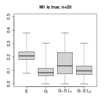
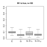
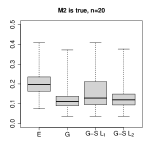
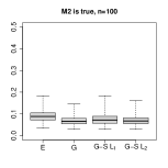
Figure 1: The boxplots of $1000$ $\ell_{2}$-distances for the empirical estimator $(E)$, Grenander estimator $(G)$, Grenander-Stone estimator with $L_{1}$ penalization (G–S $L_{1}$) and Grenander-Stone estimator with $L_{2}$ penalization (G–S $L_{2})$ for the models M1 and M2

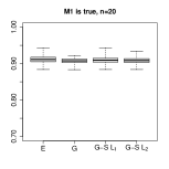
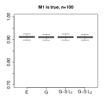
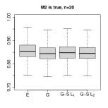
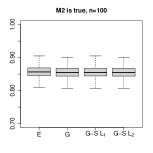
Figure 2: The boxplots of $1000$ expected $S_{2}$-scores for the empirical estimator $(E)$, Grenander estimator $(G)$, Grenander-Stone estimator with $L_{1}$ penalization (G–S $L_{1}$) and Grenander-Stone estimator with $L_{2}$ penalization (G–S $L_{2})$ for the models M1 and M2

The performance of Stone-Grenander estimator for a decreasing underlying distribution is illustrated at Figures 1 and 2. From Figure 1 one can see that Grenander-Stone estimator performs better with $L_{2}$ penalization than with $L_{1}$, and it performs better than the empirical estimator and almost as good as Grenander estimator. Also, Grenander-Stone estimator does not increase the expected $S_{2}$ score, therefore, it does not make forecast worst with respect to the empirical and Grenander estimators.

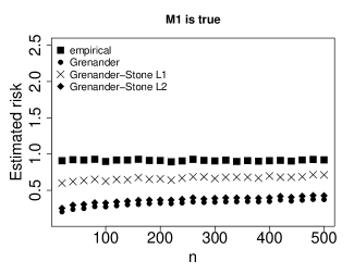
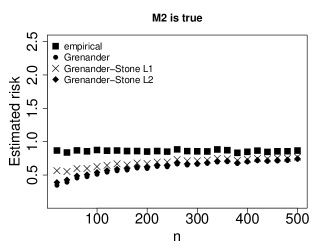
Figure 3: The estimates of the scaled risk for the models M1 and M2.

5.1.2 True distribution is not decreasing

Now let us consider the cases when the underlying distribution is not decreasing:

$$M3:\bm{p} = NBin(7,0.4),$$

$$M4:\bm{p} = \frac{3}{8}Pois(2)+\frac{5}{8}Pois(15).$$

The performance of Stone-Grenander estimator for non-monotone true distributions is presented at Figures 4 and 5. From Figure 4 it follows, first, Grenander-Stone estimator for the case of $L_{2}$ penalization is the overall winner in a sence of $\ell_{2}$ distance. Second, Grenander estimator has a better performance than the empirical estimator for a small data set. The same effect holds for stacked Grenander estimator (Pastukhov, 2022). This can be explained by reduction of the variance by isotonization, which compensates the bias in the case of small sized data sets. Next, in a sense of forecast, the winner is Grenander-Stone estimator with $L_{1}$ penalization, it performs better than Grenander-Stone estimator with $L_{2}$ penalization and Grenander estimator.

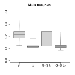
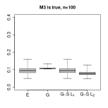
Figure 4: The boxplots of $1000$ $\ell_{2}$-distances for the empirical estimator $(E)$, Grenander estimator $(G)$, Grenander-Stone estimator with $L_{1}$ penalization (G–S $L_{1}$) and Grenander-Stone estimator with $L_{2}$ penalization (G–S $L_{2}$) for the models M3 and M4

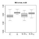
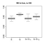
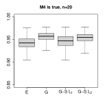
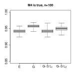
Figure 5: The boxplots of $1000$ expected $S_{2}$-scores for the empirical estimator $(E)$, Grenander estimator $(G)$, Grenander-Stone estimator with $L_{1}$ penalization (G–S $L_{1}$) and Grenander-Stone estimator with $L_{2}$ penalization (G–S $L_{2})$ for the models M3 and M4

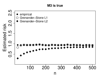
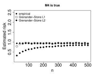
Figure 6: The estimates of the scaled risk for the models M3 and M4.

5.2 Performance of the global confidence band

In the Table 1 we provide the empirical coverage probabilities for the proposed global confidence bands of the Grenander-Stone estimator, i.e. the table shows the proportion of times that

$$\max\Big{(}(\hat{\theta}_{n,j}-\frac{\hat{q}_{\alpha}}{\sqrt{n}}),0\Big{)}\leq p_{j}\leq\hat{\theta}_{n,j}+\frac{\hat{q}_{\alpha}}{\sqrt{n}},\,\text{for all }j\in\mathbb{N}$$

among 1000 runs. The quantiles $\hat{q}_{\alpha}$ are estimated based on 100000 Monte-Carlo simulations.

Estimator	Sample size	M1	M2	M3	M4
Empirical estimator	n=100	0.958	0.95	0.973	0.97
	n=1000	0.952	0.952	0.945	0.957
	n=5000	0.945	0.944	0.951	0.953
Grenander-Stone estimator, $L_{1}$	n=100	0.959	0.966	0.973	0.97
	n=1000	0.953	0.955	0.945	0.955
	n=5000	0.952	0.944	0.952	0.953
Grenander-Stone estimator, $L_{2}$	n=100	0.991	0.98	0.997	0.997
	n=1000	0.984	0.955	0.959	0.964
	n=5000	0.981	0.944	0.959	0.957

Table 1: Empirical coverage probabilities for the confidence bands for $\alpha=0.05$.

6 Application to the real data

In this section we apply Grenander-Stone estimator to the data of the time periods from the onset of the symptoms to the notification of disease (Data set A) and time periods from notification to death (Data set B) for visceral leishmaniasis in Brazil collected from $2007$ to $2014$ (Maia-Elkhoury et al., 2019).

In the case of Data set A, Grenander-Stone estimator with $L_{1}$ penalization coincides with the empirical estimator, i.e. $\beta^{(L_{1})}=0$, while in the case of $L_{2}$ penalization the mixture parameter is $\beta^{(L_{2})}=0.28$. For Data set B, $\beta^{(L_{1})}=1$ and $\beta^{(L_{2})}=1$, therefore, Grenander-Stone estimator for both $L_{1}$ and $L_{2}$ losses coincides with Grenander estimator.

The estimators for Data sets A and B together with 95% asymptotic global confidence bands are shown in the Figure 7.

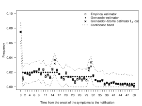
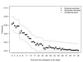
Figure 7: The frequency distribution of the time periods from onset of the symptoms to the notification of disease (left panel), and from the notification to the death. The sample size is $n=1589$, the largest order statistic is $t_{n}=1207$, the range of the distribution shown on the plot is $j\in[0,50]$.

7 Discussion and future directions

The main conclusion of this paper is that Grenander-Stone estimator is computationally feasible and it has a good performance even for small data sets, while it is less restrictive than Grenander estimator. As noted in Stone (1974), it is difficult to compare the performance $L_{1}$ and $L_{2}$ penalization. The case of $L_{1}$ penalization gives either empirical estimator or monotonically constrained Grenander estimator, while $L_{2}$ penalization mostly provides a mixture of the estimators.

The possible generalization of Grenander-Stone estimator is stacking of the empirical estimator with other shape constrained estimators, such as unimodal or convex maximum likelihood estimators. Second, the current approach can be applied to the histogram estimation of continuous distributions. Another direction of the research is stacking of constrained estimator based on other loss functions.

Appendix

Proof of Theorem 1. We consider the cases of $L_{1}$ and $L_{2}$ losses separately.

The case of $L_{1}$ loss. Recall the definitions of $\hat{\bm{\theta}}^{\backslash(i)}_{n}$ and $\hat{\bm{\theta}}^{\backslash[j]}_{n}$ at (3) and (4). Next, when $z_{i}=j\ (j=0,\dots,t_{n})$, then there exists $\bm{\delta}^{(i)}=\bm{\sigma}^{[j]}$, for some $i\ (i=1,\dots,n)$, where $\sigma^{[j]}$ defined in (2). Following the derivation in Stone (1974), for the $L_{1}$ loss the leave-one-out cross-validation criterion $C_{1}(\beta)$ is given by

$$CV_{1}(\beta)={} \frac{1}{n}\sum_{i=1}^{n}L_{1}(\bm{\delta}^{(i)},\hat{\bm{\theta}}^{\backslash(i)}_{n})=\frac{1}{n}\sum_{i=1}^{n}||\bm{\delta}^{(i)}-\hat{\bm{\theta}}^{\backslash(i)}_{n}||_{1}=\frac{1}{n}\sum_{j=0}^{t_{n}}x_{j}||\bm{\sigma}^{[j]}-\hat{\bm{\theta}}^{\backslash[j]}_{n}||_{1}=$$

$$\frac{1}{n}\sum_{j=0}^{t_{n}}x_{j}\big{[}\big{\{}1-\beta\hat{g}^{\backslash[j]}_{n,j}-(1-\beta)\frac{x_{j}-1}{n-1}\big{\}}+\sum_{k\neq j}^{t_{n}}\big{\{}\beta\hat{g}^{\backslash[j]}_{n,k}-(1-\beta)\frac{x_{k}}{n-1}\big{\}}\big{]}.$$

After the simplification we obtain

$$CV_{1}(\beta)=\frac{2}{n(n-1)}\beta\Big{[}\sum_{j=0}^{t_{n}}\big{\{}(x_{j}-n\hat{g}^{\backslash[j]}_{n,j})^{2}+(n+1)\hat{g}^{\backslash[j]}_{n,j}(x_{j}-n\hat{g}^{\backslash[j]}_{n,j})+n(\hat{g}^{\backslash[j]}_{n,j})^{2}\big{\}}-n\Big{]}+c_{1},$$

where the term $c_{1}$ does not depend on $\beta$. Therefore, the result of Theorem 1 for $L_{1}$ loss follows.

The case of $L_{2}$ loss. For the leave-one-out cross-validation criterion in the case of $L_{2}$ loss we have

$$CV_{2}(\beta)={} \frac{1}{n}\sum_{i=1}^{n}L_{2}(\bm{\delta}^{(i)},\hat{\bm{\theta}}^{\backslash(i)}_{n})=\frac{1}{n}\sum_{i=1}^{n}||\bm{\delta}^{(i)}-\hat{\bm{\theta}}^{\backslash(i)}_{n}||_{2}^{2}=\frac{1}{n}\sum_{j=0}^{t_{n}}x_{j}||\bm{\sigma}^{[j]}-\hat{\bm{\theta}}^{\backslash[j]}_{n}||_{2}^{2}=$$

$$\frac{1}{n}\sum_{j=0}^{t_{n}}x_{j}\big{[}\big{\{}1-\beta\hat{g}^{\backslash[j]}_{n,j}-(1-\beta)\frac{x_{j}-1}{n-1}\big{\}}^{2}+\sum_{k\neq j}^{t_{n}}\big{\{}\beta\hat{g}^{\backslash[j]}_{n,k}+(1-\beta)\frac{x_{k}}{n-1}\big{\}}^{2}\big{]}.$$

Then, after simplification we get

$$CV_{2}(\beta)=\frac{1}{n(n-1)^{2}}(a_{n}\,\beta^{2}-2b_{n}\,\beta)+c_{2},$$

where the term $c_{2}$ does not depend on $\beta$, and

$$a_{n}={} \sum_{j=0}^{t_{n}}x_{j}\big{[}\big{(}x_{j}-1-\hat{g}^{\backslash[j]}_{n,j}(n-1)\big{)}^{2}+\sum_{k\neq j}^{t_{n}}\big{(}x_{k}-\hat{g}^{\backslash[j]}_{n,k}(n-1)\big{)}^{2}\big{]}=$$

$$n-\sum_{j=0}^{t_{n}}\big{[}2x_{j}(x_{j}-\hat{g}^{\backslash[j]}_{n,j}(n-1))-x_{j}\sum_{k=0}^{t_{n}}(x_{k}-(n-1)\hat{g}^{\backslash[j]}_{n,k})^{2}\big{]},$$

and

$$b_{n}={} \sum_{j=0}^{t_{n}}x_{j}\big{[}\Big{\{}\sum_{k\neq j}^{t_{n}}x_{k}(x_{k}-\hat{g}^{\backslash[j]}_{n,k}(n-1))\Big{\}}-(n-x_{j})(x_{j}-\hat{g}^{\backslash[j]}_{n,j}(n-1)-1)\big{]}=$$

$$n^{2}-\sum_{j=0}^{t_{n}}x_{j}^{2}+(n-1)\sum_{j=0}^{t_{n}}x_{j}\sum_{k=0}^{t_{n}}x_{k}(\hat{g}^{\backslash[k]}_{n,k}-\hat{g}^{\backslash[j]}_{n,k}).$$

First, from the derivation of $a_{n}$ it follows that $a_{n}\geq 0$. Therefore, when $a_{n}>0$ the maximum of $CV_{2}(\beta)$ is achieved when

$$\beta^{(L_{2})}=\begin{cases}\frac{b_{n}}{a_{n}},&\text{if }\,0\leq b_{n}\leq a_{n},\\ 0,&\text{if }\,b_{n}<0,\\ 1,&\text{otherwise}.\end{cases}$$

Next, unlike the case of a constant $\bm{\lambda}$ in Stone estimator $\hat{\bm{p}}^{S}_{n}$, in our case both coefficients $a_{n}$ and $b_{n}$ can be zero. Indeed, $a_{n}=0$ when

$$\big{[}\big{(}x_{j}-1-\hat{g}^{\backslash[j]}_{n,j}(n-1)\big{)}^{2}+\sum_{k\neq j}^{t_{n}}\big{(}x_{k}-\hat{g}^{\backslash[j]}_{n,k}(n-1)\big{)}^{2}\big{]}=0,$$

for all $j=0,\dots,t_{n}$. Therefore, $a_{n}=0$ iff for all $j=0,\dots,t_{n}$

$$\begin{cases}\hat{g}^{\backslash[j]}_{n,k}=\frac{x_{k}-1}{n-1},&\text{if}\,k=j,\\ \hat{g}^{\backslash[j]}_{n,k}= \frac{x_{k}}{n-1},&\text{if}\,k\neq j,\end{cases}$$

which is equivalent to

$$\bm{g}^{\backslash[j]}_{n}\equiv\Pi\big{(}\frac{\bm{x}-\bm{\sigma}^{[j]}}{n-1}\mid\mathcal{F}^{decr}\big{)}=\frac{\bm{x}-\bm{\sigma}^{[j]}}{n-1},$$ (9)

for all $j=0,\dots,t_{n}$. If the condition (9) is satisfied, then also $b=0$. For any vector $\bm{f}\in\ell_{2}$ we have $\Pi(\bm{f}\mid\mathcal{F}^{is})=\bm{f}$ iff $\bm{f}$ is a decreasing vector. Therefore, in order to satisfy the condition in (9), the frequency vector $x$, and, consequently, the empirical estimator $\hat{\bm{p}}_{n}$ must be strictly decreasing. Next, if $x$ is strictly decreasing, then $\hat{\bm{\theta}}_{n}=\hat{\bm{p}}_{n}$, and for consistency of notation we can set $\beta=0$. Finally, we obtain the following result for $\beta^{(L_{2})}_{n}$:

$$\beta^{(L_{2})}_{n}=\begin{cases}\frac{b_{n}}{a_{n}},&\text{if }\,a_{n}\neq 0\text{ and }0\leq b_{n}\leq a_{n},\\ 0,&\text{if }\,a_{n}=0\text{ or }b_{n}<0,\\ 1,&\text{otherwise}.\end{cases}$$

$\Box$

Proof of Theorem 2. First, let us assume that the underlying distribution $\bm{p}$ is decreasing. Next, from (6), and since in this case both $\hat{\bm{g}}_{n}$ and $\hat{\bm{p}}_{n}$ are strongly consistent in $\ell_{k}$-norm $(1\leq k\leq\infty)$ with $\sqrt{n}$-rate of convergence, cf. Theorem 2.4 and Corollary 4.1 in Jankowski & Wellner (2009), and $0\leq\hat{\beta}^{(L_{d})}_{n}\leq 1$ for all $n$, then the strongly consistency and $\sqrt{n}$-rate of convergence hold trivially,

Next, let us assume that $\bm{p}$ is not decreasing. We consider the cases of $L_{1}$ and $L_{2}$ losses separately.

The case of $L_{1}$ loss. Let us define the sequence of vectors $\hat{\bm{\gamma}}_{n}\in\ell_{1}$ as

$$\hat{\gamma}_{n,j}=\begin{cases}\hat{g}^{\backslash[j]}_{n,j},&\text{if }\,x_{j}>0,\\ 0,&\text{otherwise}.\end{cases}$$

Then, from Theorem 2 in Pastukhov (2022) it follows that $\hat{\bm{\gamma}}_{n}\stackrel{{\scriptstyle a.s.}}{{\to}}\bm{g}$ in $\ell_{k}$-norm $(1\leq k\leq\infty)$.

Recall the definition of $\beta^{(L_{1})}_{n}$ at Theorem 1. Let us rewrite $\beta^{(L_{1})}_{n}$ as

$$\beta^{(L_{1})}_{n}=\begin{cases}0,&\text{if }B_{n}\geq n,\\ 1,&\text{otherwise},\end{cases}$$

where

$$B_{n}= \sum_{j=0}^{t_{n}}(x_{j}-n\hat{\gamma}_{n,j})^{2}+\sum_{j=0}^{t_{n}}(n+1)\hat{\gamma}_{n,j}(x_{j}-n\hat{\gamma}_{n,j})+\sum_{j=0}^{t_{n}}n(\hat{\gamma}_{n,j})^{2}\equiv B_{n}^{(1)}+B_{n}^{(2)}+B_{n}^{(3)}.$$

Next, from continuous mapping theorem, almost sure convergence of $\hat{\bm{\gamma}}_{n}$, Lemma 1 in Pastukhov (2022) and properties of isotonic regression it follows that

$$B_{n}^{(1)}/n^{2}\stackrel{{\scriptstyle a.s.}}{{\to}}||(\bm{p}-\bm{g})||_{2}^{2}>0,\quad B_{n}^{(2)}/n^{2}\stackrel{{\scriptstyle a.s.}}{{\to}}\langle\bm{g},(\bm{p}-\bm{g})\rangle=0,\quad\text{and}\quad B_{n}^{(3)}/n^{2}\stackrel{{\scriptstyle a.s.}}{{\to}}0.$$

We have shown that $B_{n}/n^{2}\stackrel{{\scriptstyle a.s.}}{{\to}}||(\bm{p}-\bm{g})||_{2}^{2}$, which means that there exists sufficiently large random $n_{0}$ such that $B_{n}>n$ for all $n>n_{0}$ almost surely and, therefore, $\beta^{(L_{1})}_{n}=0$ for all $n>n_{0}$ almost surely, which provides that $\hat{\bm{\theta}}_{n}=\hat{\bm{p}}_{n}$, for all $n>n_{0}$ almost surely. The strong consistency of $\hat{\bm{\theta}}_{n}$ now follows from strong consistency of the empirical estimator $\hat{\bm{p}}_{n}$.

Finally, the result for the rate of convergence of $\hat{\bm{\theta}}_{n}$ follows from the rate of convergence of the empirical estimator i.e. as proved in Corollaries 4.1 and 4.2. in Jankowski & Wellner (2009)

$$n^{1/2}||\hat{\bm{p}}_{n}-\bm{p}||_{k}=O_{p}(1)\quad(2\leq k\leq\infty),$$

and, if in addition $\sum_{j=0}^{\infty}\sqrt{p}_{j}<\infty$ holds, then

$$n^{1/2}||\hat{\bm{p}}_{n}-\bm{p}||_{1}=O_{p}(1).$$

The case of $L_{2}$ loss. Recall the definitions of $a_{n}$ and $b_{n}$ at Theorem 1. Let us start with the asymptotic properties of $a_{n}$. Let us rewrite $a_{n}$ as

$$a_{n}=\mathfrak{a}^{(1)}_{n}+\mathfrak{a}^{(2)}_{n},$$

where

$$\mathfrak{a}^{(1)}_{n}=n-2\sum_{j=0}^{t_{n}}x_{j}(x_{j}-\hat{g}^{\backslash[j]}_{n,j}(n-1)),\quad\mathfrak{a}^{(2)}_{n}=\sum_{j=0}^{t_{n}}x_{j}\sum_{k=0}^{t_{n}}(x_{k}-(n-1)\hat{g}^{\backslash[j]}_{n,k})^{2}.$$

First, from continuous mapping theorem, almost sure convergence of $\hat{\bm{\gamma}}_{n}$ and the property of $\ell_{2}$ projection onto the cone we have $\mathfrak{a}^{(1)}_{n}/n^{2}\stackrel{{\scriptstyle a.s.}}{{\to}}-2\langle\bm{p},(\bm{p}-\bm{g})\rangle<0$. Second, for any fixed $j$ we have $\hat{\bm{g}}^{\backslash[j]}_{n}\stackrel{{\scriptstyle a.s.}}{{\to}}\bm{g}$. Furthermore, since $\bm{g}\neq\bm{p}$, if $\bm{p}$ is not decreasing, then there exists sufficiently large random $n_{0}$ such that $\mathfrak{a}^{(2)}_{n}/n^{3}>0$ for all $n>n_{0}$ almost surely. Therefore, there exists sufficiently large random $n_{1}$ such that $a_{n}/n^{3}>0$, for all $n>n_{1}$ almost surely.

Next, we study the asymptotic properties of $b_{n}$. Let us rewrite $b_{n}$ as

$$b_{n}=\mathfrak{b}^{(1)}_{n}+\mathfrak{b}^{(2)}_{n},$$

where

$$\mathfrak{b}^{(1)}_{n}=n^{2}-\sum_{j=0}^{t_{n}}x_{j}^{2},\quad\mathfrak{b}^{(2)}_{n}=(n-1)\sum_{j=0}^{t_{n}}x_{j}\sum_{k=0}^{t_{n}}x_{k}(\hat{g}^{\backslash[k]}_{n,k}-\hat{g}^{\backslash[j]}_{n,k}).$$

First, note that $\mathfrak{b}^{(1)}_{n}/n^{2.5}\stackrel{{\scriptstyle a.s.}}{{\to}}0$. Second, from the contraction property of a simple isotonic regression with respect to sup-norm, (cf. Lemma 1 in Yang & Barber (2019)), for any $j$ we have

$$\sup_{k}|\hat{g}^{\backslash[k]}_{n,k}-\hat{g}^{\backslash[j]}_{n,k}|\leq\sup_{k}|\hat{p}^{\backslash[k]}_{n,k}-\hat{p}^{\backslash[j]}_{n,k}|=\frac{1}{n-1}.$$

Therefore, for $\mathfrak{b}^{(2)}_{n}$ we have

$$|\mathfrak{b}^{(2)}_{n}|\leq(n-1)\sum_{j=0}^{t_{n}}x_{j}\sum_{k=0}^{t_{n}}x_{k}\frac{1}{n-1}=n^{2},$$

which yields $b_{n}/n^{2.5}\stackrel{{\scriptstyle a.s.}}{{\to}}0$. Third, since $\beta^{(L_{2})}_{n}\geq 0$, then it follows that

$$n^{1/2}\beta^{(L_{2})}_{n}\stackrel{{\scriptstyle a.s.}}{{\to}}0.$$ (10)

Finally, the inequality (6) and the strong consistency of the empirical estimator $\hat{\bm{p}}_{n}$ yields strong consistency of Grenander-Stone estimator for the case of $L_{2}$ loss penalization. The $n^{1/2}$-rate of convergence follows from (10) and the $n^{1/2}$-rate of convergence of the empirical estimator. $\Box$

Proof of Proposition 1. Let us consider some arbitrary $\bm{h}\in\mathcal{P}$ and let $t\leq\infty$ be the size of support of $\bm{h}$. Recall the definition of $S_{1}(\bm{f},\bm{p})$ at (7). Then

$$S_{1}(\bm{f},\bm{p})=2-\sum_{k=0}^{t}p_{k}(\beta h_{k}+(1-\beta)p_{k})=2-\beta\sum_{k=0}^{t}p_{k}(h_{k}-p_{k})+||\bm{p}||_{2}^{2}.$$ (11)

Next, since $\sum_{k=0}^{t}p_{k}(h_{k}-p_{k})\geq 0$, then $S_{1}(\bm{f},\bm{p})$ is minimised by $\beta=0$, which yields $\bm{f}=\bm{p}$.

Proof of Theorem 3. First, note that from the max-min formulas in (1) it follows that

$$\sup\{j:\hat{g}_{n,j}>0\}=\sup\{j:\hat{p}_{n,j}>0\}\equiv t_{n}$$ (12)

for any $n$. Next, let $D_{j}$ be a cumulative sum function of any decreasing distribution on $\mathbb{N}$. From (12) it follows that for a given sample $\mathcal{Z}_{n}$ we have

$$\sup_{j\in[t_{n}+1,\infty]}||\hat{F}^{G}_{n,j}-D_{j}||_{\infty}=\sup_{j\in[t_{n}+1,\infty]}||\hat{F}_{n,j}-D_{j}||_{\infty}=\sup_{j\in[t_{n}+1,\infty]}|1-D_{j}|,$$

where $\hat{F}_{n,j}=\sum_{k=0}^{j}\hat{p}_{n,j}\ (j\in\mathbb{N})$, and $\hat{F}^{G}_{n,j}=\sum_{k=0}^{j}\hat{g}_{n,j}\ (j\in\mathbb{N})$.

Second, let $\hat{F}_{n,j}^{GS}=\sum_{k=0}^{j}\hat{\theta}_{n,j}\ (j\in\mathbb{N})$, and note that from the subadditivity of norms it follows that

$$\sup_{j\in\mathbb{N}}||\hat{F}_{n,j}^{GS}-D_{j}||_{\infty}\leq\beta^{L_{d}}_{n}\sup_{j\in\mathbb{N}}||\hat{F}^{G}_{n,j}-D_{j}||_{\infty}+(1-\beta^{L_{d}}_{n})\sup_{j\in\mathbb{N}}||\hat{F}_{n,j}-D_{j}||_{\infty}.$$

Third, from Lemma in Section 2.2 in Brunk et al. (1972) it follows that for a cumulative sum function $D_{j}$ of any decreasing probability vector we have

$$\sup_{j\in[0,t_{n}]}||\hat{F}^{G}_{n,j}-D_{j}||_{\infty}\leq\sup_{j\in[0,t_{n}]}||\hat{F}_{n,j}-D_{j}||_{\infty},$$

which completes the proof. $\Box$

Proof of Proposition 2. From Proposition B.7 at Balabdaoui & Jankowski (2016) it follows that we have to prove:
(a) $\hat{\bm{\theta}}_{n}$ converges to $\bm{p}$ point-wise almost surely,
(b) $\lim_{m\to\infty}\lim_{n\to\infty}\sum_{j>m}\hat{\theta}_{n,j}=0$.

The Condition (a) follows from Theorem 2. Let us prove the Condition (b). Let $\hat{F}_{n,j}\ (j\in\mathbb{N})$, be the empirical distribution function, let $\hat{F}_{n,j}^{G}=\sum_{k=0}^{j}\hat{g}_{n,j}\ (j\in\mathbb{N})$, and $\hat{F}_{n,j}^{GS}=\sum_{k=0}^{j}\hat{\theta}_{n,j}\ (j\in\mathbb{N})$.

Next, from the properties of a simple order isotonic regression it follows that $\hat{F}_{n,j}^{GS}$ is given by the least concave majorant of $\hat{F}_{n,j}$ (Brunk et al., 1972; Robertson & Wright, 1980). Therefore, we have $\hat{F}_{n,j}^{G}\geq\hat{F}_{n,j}$ for any $j$ and $n$. Therefore,

$$\sum_{j>m}\hat{\theta}_{n,j}=1-\hat{F}_{n,m}^{GS}=1-\beta^{(L_{d})}_{n}\hat{F}_{n,j}^{G}-(1-\beta^{(L_{d})}_{n})\hat{F}_{n,j}\leq 1-\hat{F}_{n,m}\quad(d=1,2),$$

and from the properties of the empirical distribution function it follows $\lim_{m\to\infty}\lim_{n\to\infty}(1-\hat{F}_{n,m})=0$ almost surely. $\Box$

References

• (1)
• Balabdaoui & Durot (2015) Balabdaoui, F. & Durot, C. (2015), ‘Marshall lemma in discrete convex estimation’, Statistics & Probability Letters 99, 143–148.
• Balabdaoui et al. (2017) Balabdaoui, F., Durot, C. & Koladjo, F. (2017), ‘On asymptotics of the discrete convex lse of a pmf’, Bernoulli 23(3), 1449–1480.
• Balabdaoui & Jankowski (2016) Balabdaoui, F. & Jankowski, H. (2016), ‘Maximum likelihood estimation of a unimodal probability mass function’, Statistica Sinica pp. 1061–1086.
• Balabdaoui et al. (2013) Balabdaoui, F., Jankowski, H., Rufibach, K. & Pavlides, M. (2013), ‘Asymptotics of the discrete log-concave maximum likelihood estimator and related applications’, Journal of the Royal Statistical Society: SERIES B: Statistical Methodology pp. 769–790.
• Bowman et al. (1984) Bowman, A. W., Hall, P. & Titterington, D. (1984), ‘Cross-validation in nonparametric estimation of probabilities and probability densities’, Biometrika 71(2), 341–351.
• Brunk et al. (1972) Brunk, H., Barlow, R. E., Bartholomew, D. J. & Bremner, J. M. (1972), Statistical inference under order restrictions (the theory and application of isotonic regression), Technical report, Missouri Univ Columbia Dept of Statistics.
• Buja et al. (2005) Buja, A., Stuetzle, W. & Shen, Y. (2005), ‘Loss functions for binary class probability estimation and classification: Structure and applications’, Working draft, November 3.
• Czado et al. (2009) Czado, C., Gneiting, T. & Held, L. (2009), ‘Predictive model assessment for count data’, Biometrics 65(4), 1254–1261.
• Dümbgen et al. (2007) Dümbgen, L., Rufibach, K. & Wellner, J. A. (2007), Marshall’s lemma for convex density estimation, in ‘Asymptotics: particles, processes and inverse problems’, Institute of Mathematical Statistics, pp. 101–107.
• Durot et al. (2013) Durot, C., Huet, S., Koladjo, F. & Robin, S. (2013), ‘Least-squares estimation of a convex discrete distribution’, Computational Statistics & Data Analysis 67, 282–298.
• Fienberg & Holland (1972) Fienberg, S. E. & Holland, P. W. (1972), ‘On the choice of flattening constants for estimating multinomial probabilities’, Journal of Multivariate Analysis 2(1), 127–134.
• Fienberg & Holland (1973) Fienberg, S. E. & Holland, P. W. (1973), ‘Simultaneous estimation of multinomial cell probabilities’, Journal of the American Statistical Association 68(343), 683–691.
• Haghtalab et al. (2019) Haghtalab, N., Musco, C. & Waggoner, B. (2019), ‘Toward a characterization of loss functions for distribution learning’, arXiv preprint arXiv:1906.02652 .
• Hastie et al. (2020) Hastie, T., Tibshirani, R. & Tibshirani, R. (2020), ‘Best subset, forward stepwise or lasso? analysis and recommendations based on extensive comparisons’, Statistical Science 35(4), 579–592.
• Jankowski & Wellner (2009) Jankowski, H. K. & Wellner, J. A. (2009), ‘Estimation of a discrete monotone distribution’, Electronic journal of statistics 3, 1567.
• Jankowski & Tian (2018) Jankowski, H. & Tian, Y. H. (2018), ‘Estimating a discrete log-concave distribution in higher dimensions’, Statistica Sinica 28(4), 2697–2712.
• Maia-Elkhoury et al. (2019) Maia-Elkhoury, A. N. S., Sierra Romero, G. A., OB Valadas, S. Y., L. Sousa-Gomes, M., Lauletta Lindoso, J. A., Cupolillo, E., Ruiz-Postigo, J. A., Argaw, D. & Sanchez-Vazquez, M. J. (2019), ‘Premature deaths by visceral leishmaniasis in brazil investigated through a cohort study: A challenging opportunity?’, PLoS neglected tropical diseases 13(12), e0007841.
• Minami (2020) Minami, K. (2020), ‘Estimating piecewise monotone signals’, Electronic Journal of Statistics 14(1), 1508–1576.
• Pastukhov (2022) Pastukhov, V. (2022), ‘Stacked grenander and rearrangement estimators of a discrete distribution’, Electronic Journal of Statistics 16(2), 4247–4274.
• Rigollet & Tsybakov (2007) Rigollet, P. & Tsybakov, A. B. (2007), ‘Linear and convex aggregation of density estimators’, Mathematical Methods of Statistics 16(3), 260–280.
• Robertson & Wright (1980) Robertson, T. & Wright, F. T. (1980), ‘Algorithms in order restricted statistical inference and the cauchy mean value property’, The Annals of Statistics pp. 645–651.
• Smyth & Wolpert (1999) Smyth, P. & Wolpert, D. (1999), ‘Linearly combining density estimators via stacking’, Machine Learning 36(1), 59–83.
• Stone (1974) Stone, M. (1974), ‘Cross-validation and multinomial prediction’, Biometrika 61(3), 509–515.
• Tibshirani et al. (2011) Tibshirani, R. J., Hoefling, H. & Tibshirani, R. (2011), ‘Nearly-isotonic regression’, Technometrics 53(1), 54–61.
• Trybula (1958) Trybula, S. (1958), ‘Some problems of simultaneous minimax estimation’, The Annals of Mathematical Statistics 29(1), 245–253.
• Yang & Barber (2019) Yang, F. & Barber, R. F. (2019), ‘Contraction and uniform convergence of isotonic regression’, Electronic Journal of Statistics 13(1), 646–677.