Distributional Adaptive Soft Regression Trees

Umlauf N., Klein N. Distributional Adaptive Soft Regression Trees Distributional Adaptive Soft Regression Trees Random forests are an ensemble method relevant for many problems, such as regression or classification. They are popular due to their good predictive performance (compared to, e.g., decision trees) requiring only minimal tuning of hyperparameters. They are built via aggregation of multiple regression trees during training and are usually calculated recursively using hard splitting rules. Recently regression forests have been incorporated into the framework of distributional regression, a nowadays popular regression approach aiming at estimating complete conditional distributions rather than relating the mean of an output variable to input features only – as done classically. This article proposes a new type of a distributional regression tree using a multivariate soft split rule. One great advantage of the soft split is that smooth high-dimensional functions can be estimated with only one tree while the complexity of the function is controlled adaptive by information criteria. Moreover, the search for the optimal split variable is obsolete. We show by means of extensive simulation studies that the algorithm has excellent properties and outperforms various benchmark methods, especially in the presence of complex non-linear feature interactions. Finally, we illustrate the usefulness of our approach with an example on probabilistic forecasts for the Sun’s activity. Adaptive soft split; decision trees; generalized additive models for location, scale and shape; probabilistic forecasting, random forests Adaptive soft split; decision trees; generalized additive models for location, scale and shape; probabilistic forecasting, random forests Nikolaus Umlauf
Department of Statistics
Faculty of Economics and Statistics
Universität Innsbruck
Universitätsstr. 15
6020 Innsbruck, Austria
E-mail: ,
URL: https://eeecon.uibk.ac.at/~umlauf/,
Nadja Klein
Humboldt Universität zu Berlin
School of Business and Economics
Chair of Statistics and Data Science
Unter den Linden 6
10099 Berlin, Germany
E-mail:
URL: https://hu.berlin/NK

1 Introduction

In many applications it is important to model not only the expected value of a response variable, but rather a complete probabilistic prediction model. While there have been proposed numerous methods to obtain such an also called distributional model (see e.g.  Kneib et al., 2021, for a recent review), in this paper we focus on the class of structured additive distributional regression (Klein et al., 2015a) aka generalized additive model for location, scale and shape (GAMLSS; Rigby and Stasinopoulos, 2005), which can model every parameter of an arbitrary parametric target distribution through input features thereby implicitly constituting a probabilistic prediction model. This model class has been successfully used in a number of applications to develop state-of-the-art probabilistic forecasts (see, e.g., Klein et al., 2014; Simon et al., 2018, 2019; Consortium, 2020; Serinaldi, 2011; Ziel, 2021). In GAMLSS, each distribution parameter is typically modeled with a structured additive predictor (STAR; Fahrmeir et al., 2013; Wood, 2017) decomposed from a sum of smooth generic functions, following the structure of generalized additive models (GAM; Hastie and Tibshirani, 1990). Although this class of models can already model fairly complex interactions, the ability to estimate higher dimensional functions with, for example, more than three features using (tensor product) splines is very difficult and costly, since, for example, the number of parameters to be estimated increases exponentially with each additional input variable. To address this issue, distribution trees and forests have recently been proposed by Schlosser et al. (2019), which are based on split methods similar to the very established random forests (Breiman, 2001, RF). In a similar vein, Rügamer et al. (2021) propose to extend the STAR predictors of each distributional parameter by a deep neural network to allow for high-dimensional interaction terms and where identification is realized through a generic orthogonalization cell. Although RFs are known for their high flexibility, the splitting method is still a limiting factor in modeling smooth high-dimensional functions. The reason is relatively simple: a single regression tree is usually built using hard splits, which lead to a tree modeling a step function. This in turn means that an RF, which consists of a number of trees, will in the best case find only a “nearly smooth function”. The step function approximation problem can sometimes be exacerbated when there are larger gaps in the data and many covariates. Although Breiman (2001) provides an upper bound on the generalization error and Probst and Boulesteix (2018) more recently show empirically and theoretically that increasing the size of an RF is beneficial, the approximation error as a consequence of the splitting rule is not considered. Ciampi et al. (2002) first addressed this problem by instead using a soft probabilistic splitting rule for growing a tree. This idea is followed to the best of our knowledge only by few contributions (e.g. Nguyen, 2002; Frosst and Hinton, 2017; Linero and Yang, 2018; Luo et al., 2021); but none of them considers a distributional framework. The prominence of a hard splitting rule is most likely due to the fact that a single tree yields a completely interpretable model and its robustness in mean regression applications. However, especially for distributional models RFs are usually used as predictive models, where interpretation only plays a minor role. In Irsoy et al. (2012) a multivariate version of the soft decision tree is introduced and Yıldız et al. (2016) show excellent predictive performance when bagging multivariate soft decision trees.

In this paper, we extend these ideas of soft splitting rules for the class of GAMLSS and propose a distributional adaptive soft regression tree (DAdaSoRT) for full probabilistic forecasting that is capable of approximating both linear and complex non-linear rough and smooth functions. Our main contributions are:

• A single distributional soft tree is grown using multivariate soft splits, which has in most cases better, at least similar, approximation capabilities than a complete distributional forest.

• The tree growth algorithm is adaptive and the optimal size is selected based on information criteria such as the Akaike information criterion (AIC) or Bayesian information criterion (BIC), which lead to final trees with relatively few degrees of freedom.

• To further avoid the problem of overfitting, additional shrinkage parameters control the smoothness of the estimated functions and are the only hyperparameters.

• The efficacy of our proposed method is demonstrated in a benchmark study and in a forecast exercise for predicting the Sun’s activity based on time series data.

The remainder of this paper is organized as follows: In Section 2 we first introduce the ideas of classical soft regression trees in detail before presenting the full adaptive version of a soft tree. Then, in Section 3, we extend the adaptive soft regression trees to distributional regression based on GAMLSS (referred to as DAdaSoRT) and provide algorithms for estimation. In Section 4 we present further properties and details of distributional adaptive soft regression trees. In Section 5 we briefly introduce the accompanying R package softtrees. An extensive simulation study that examines the performance of soft distributional regression trees compared to classical GAMLSS models and distributional forests is presented in Section 6. In Section 7 we then show the benefits of the approach using a complex problem of probabilistic forecasting the Sun’s solar cycles 25 and 26.

2 Adaptive Soft Regression Trees

In this section, we first review the classical multivariate soft regression trees before we introduce our improved version which we call adaptive soft regression trees (AdaSoRT) and which allows to obtain more efficient predictions through local adaptive smoothing in the model fits.

2.1 Classical Soft Regression Trees

Classical regression trees use hard binary splits as a tree grows. The exact split point is searched in different ways, e.g., by an exhaustive search or by decision rules based on instability tests (Hothorn et al., 2006). In contrast to this, soft regression trees (SoRT) are grown with so-called soft splitting rules, which means that instead of a step function a soft discriminator is used, a smooth continuous function that does not have an exact split point. Each terminal node is influenced by all observation points through the weighting created in this way.

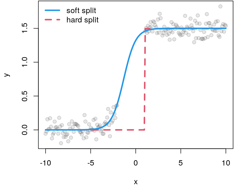
Figure 1: Illustrating example. Shown are bivariate simulated data $(y,x)$ (light-grey points) together with a classical hard split (dashed red line) and a soft split using a logistic function (blue solid line).

An example that illustrates this difference along simulated bivariate data is shown in Figure 1. Here, the hard binary split (dashed red line) separates the data at $x=1$ and yields only two possible predictions, i.e. $\hat{y}=0$ for $x<1$ and $\hat{y}=1.5$ for $x\geq 1$. Instead, the soft split (blue line) allows a smooth transition. Intuitively, rather than assigning observations to single nodes, a soft split uses a better balanced weighting of all possible nodes.

The literature differentiates between univariate and multivariate soft splits. While univariate soft splits (as, e.g., introduced by Ciampi et al., 2002, for binary outcomes) typically outperform hard splits, they still require finding the optimum split variable, which can be computationally intensive, in particular when the feature space is large. To reduce the computational burden, Irsoy et al. (2012) instead proposed a multivariate soft node which is in principal similar to the nodes of a neural network (NN). In that respect, Frosst and Hinton (2017) distil a NN into a soft decision tree to improve upon NN classification tasks and Luo et al. (2021) show that soft decision trees can be an alternative to deep NNs for numerous regression tasks.

Now suppose there is data $\text{\boldmath$y$}=(y_{1},\ldots,y_{n})^{\top}$, such that for each output $y_{i}$, $i=1,\ldots,n$ there is a $q$-dimensional feature vector $\text{\boldmath$x$}_{i}=(x_{i1},\ldots,x_{iq})^{\top}$ available. Let furthermore $\mathcal{N}=\mathcal{M}\,\dot{\cup}\,\mathcal{T}$ be the set of all nodes (excluding the root node) consisting of the disjoint union of the set of all nodes that have children (i.e., those that serve as root nodes for some others) $\mathcal{M}$ and the set of terminal (leaf) nodes $\mathcal{T}$, such that $|\mathcal{M}|=M$, $|\mathcal{T}|=T$ and $|\mathcal{N}|=M+T$. For growing a SoRT any root node $l\in\mathcal{M}$, with output $N_{l}(\cdot)$ is “split softly” into a weighted average of left and right child nodes, $N_{l}^{L}(\cdot)$ and $N_{l}^{R}(\cdot)$, respectively, where

$$N_{l}(\text{\boldmath$x$}_{i})=N_{l}^{L}(\text{\boldmath$x$}_{i})\cdot p_{l}(\text{\boldmath$x$}_{i})+N_{l}^{R}(\text{\boldmath$x$}_{i})\cdot(1-p_{l}(\text{\boldmath$x$}_{i})),$$ (1)

and the weighting function $p_{l}(\cdot)\in[0,1]$ can be seen as the posterior probability $\text{$\mathds{P}$}(L\mid\text{\boldmath$x$}_{i})=p_{l}(\text{\boldmath$x$}_{i})$ of redirecting $y_{i}$ to the left child node given $\text{\boldmath$x$}_{i}$; and $\text{$\mathds{P}$}(R\mid\text{\boldmath$x$}_{i})=1-p_{l}(\text{\boldmath$x$}_{i})$ being the corresponding probability for assignment to the right node. A common choice for the mappings $p_{l}(\cdot):\text{$\mathds{R}$}\mapsto[0,1]$ is the sigmoid (logistic) function given by

$$p_{l}(\text{\boldmath$x$}_{i})=\frac{1}{1+\exp(-(\text{\boldmath$x$}_{i}^{\top}\text{\boldmath$\omega$}_{l}))},$$ (2)

where $\text{\boldmath$\omega$}_{l}$ are weights that need to be estimated from the data. If $N_{l}^{L}(\text{\boldmath$x$}_{i})$ and $N_{l}^{R}(\text{\boldmath$x$}_{i})$ are terminal nodes, i.e. $l\in\mathcal{T}$, we can write

$$N_{l}(\text{\boldmath$x$}_{i})=\beta_{l}^{L}\cdot p_{l}(\text{\boldmath$x$}_{i})+\beta_{l}^{R}\cdot(1-p_{l}(\text{\boldmath$x$}_{i})),$$ (3)

with parameters $N_{l}^{L}(\text{\boldmath$x$}_{i})=\beta_{l}^{L}$ and $N_{l}^{R}(\text{\boldmath$x$}_{i})=\beta_{l}^{R}$ that need to be estimated, too. This means, in each SoRT growing step one of the nodes $N_{l}^{L}(\text{\boldmath$x$}_{i})$ or $N_{l}^{R}(\text{\boldmath$x$}_{i})$ is replaced by another soft split node (1) unless $l\in\mathcal{T}$. Therefore, the multiplicative soft weighting that is enforced leads to a type of basis functions that adapt to the data in a smooth way, since at each node the function is differentiable if and only if $p_{l}(\cdot)$ is differentiable. Finally, given the sets $\mathbf{\Omega}_{1},\ldots,\mathbf{\Omega}_{T}$ of weights involved in computing each of the $T$ terminal nodes as well as $\mathbf{\Omega}$ denoting the set of all weights in the tree, predictions $\hat{y}^{\ast}$ from the final SoRT for any new feature $\text{\boldmath$x$}^{\ast}$ can be computed by the linear combination $\text{\boldmath$N$}(\text{\boldmath$x$}^{\ast},\mathbf{\Omega})^{\top}\boldsymbol{\beta}$, where $\text{\boldmath$\beta$}=(\beta_{1},\ldots,\beta_{T})^{\top}$ is the vector of terminal node parameters and $\text{\boldmath$N$}(\text{\boldmath$x$}^{\ast},\mathbf{\Omega})^{\top}=(P_{1}(\text{\boldmath$x$}^{\ast},\mathbf{\Omega}_{1}),\ldots,P_{T}(\text{\boldmath$x$}^{\ast},\mathbf{\Omega}_{T}))^{\top}$ is the $T$-dimensional design vector with path probabilities for the $T$ paths in the tree. More precisely, let $D_{l}$ denote a path of length $\log_{2}(T)$ associated with $P_{l}(\text{\boldmath$x$}^{\ast},\mathbf{\Omega}_{l})$. Let furthermore $\mathcal{D}_{l}$ be the set of nodes involved in that path $D_{l}$. Then, we can write

$$P_{l}(\text{\boldmath$x$}^{\ast},\mathbf{\Omega}_{l})=\prod_{r\in\mathcal{D}_{l}}p_{r}(\text{\boldmath$x$}^{\ast})^{d_{r}}(1-p_{r}(\text{\boldmath$x$}^{\ast}))^{1-d_{r}},$$ (4)

with $d_{r}\in\{0,1\}$ indicating the binary directions (left/right) in each split along the path. In Figure 2 the construction of a SoRT is illustrated. Here, each path $D_{l}$, $l=1,\ldots,4$ from the top root node to one of the four terminal nodes represents one column of the design matrix $\text{\boldmath$N$}(\text{\boldmath$X$},\mathbf{\Omega})\in\text{$\mathds{R}$}^{n\times T}$, which are constructed by multiplication of level specific probabilities as defined in (4), and where $\text{\boldmath$X$}=(\text{\boldmath$x$}_{1}|\ldots|\text{\boldmath$x$}_{n})^{\top}$ is the $n\times q$ feature matrix. For instance, the most left path $D_{1}$ (thick black lines in Figure 2) from $p_{1}$ to $p_{2}$ to $\beta_{1}p_{1}p_{2}$ has length 2. Its involved weights are $\mathbf{\Omega}_{1}=\{\text{\boldmath$\omega$}_{1},\text{\boldmath$\omega$}_{2}\}$.

[sibling distance=10em, level distance=8em, every node/.style = shape=rectangle, rounded corners, draw=none, align=center, top color=white, ered/.style=edge from parent/.style=red,very thick,draw] Root node child node Left child node child node $\beta_{1}p_{1}(\cdot)p_{2}(\cdot)$
$d_{1}=(1,1)^{\top}$ edge from parent [black, line width=2.5pt] node[above left] $p_{2}(\text{\boldmath$x$}^{\ast},\text{\boldmath$\omega$}_{2})$ child node $\beta_{2}p_{1}(\cdot)(1-p_{2}(\cdot))$
$d_{2}=(1,0)^{\top}$ edge from parent [black, line width=0.5pt] node[above right] $1-p_{2}(\text{\boldmath$x$}^{\ast},\text{\boldmath$\omega$}_{2})$ edge from parent [black, line width=2.5pt] node[above left] $p_{1}(\text{\boldmath$x$}^{\ast},\text{\boldmath$\omega$}_{1})$ child [missing] child node Right child nodechild node $\beta_{3}(1-p_{1}(\cdot))p_{3}(\cdot)$
$d_{3}=(0,1)^{\top}$ edge from parent node[above left] $p_{3}(\text{\boldmath$x$}^{\ast},\text{\boldmath$\omega$}_{3})$ child node $\beta_{4}(1-p_{1}(\cdot))(1-p_{3}(\cdot))$
$d_{4}=(0,0)^{\top}$ edge from parent node[above right] $1-p_{3}(\text{\boldmath$x$}^{\ast},\text{\boldmath$\omega$}_{3})$ edge from parent node[above right] $1-p_{1}(\text{\boldmath$x$}^{\ast},\text{\boldmath$\omega$}_{1})$ ;

Figure 2: Illustrating tree structure. A SoRT with $4$ terminal nodes.

An illustration of the recursion for an $n$ dimensional training data set with feature matrix $X$ and designmatrix $\text{\boldmath$N$}(\text{\boldmath$X$},\mathbf{\Omega})$ is given in Figure 3.

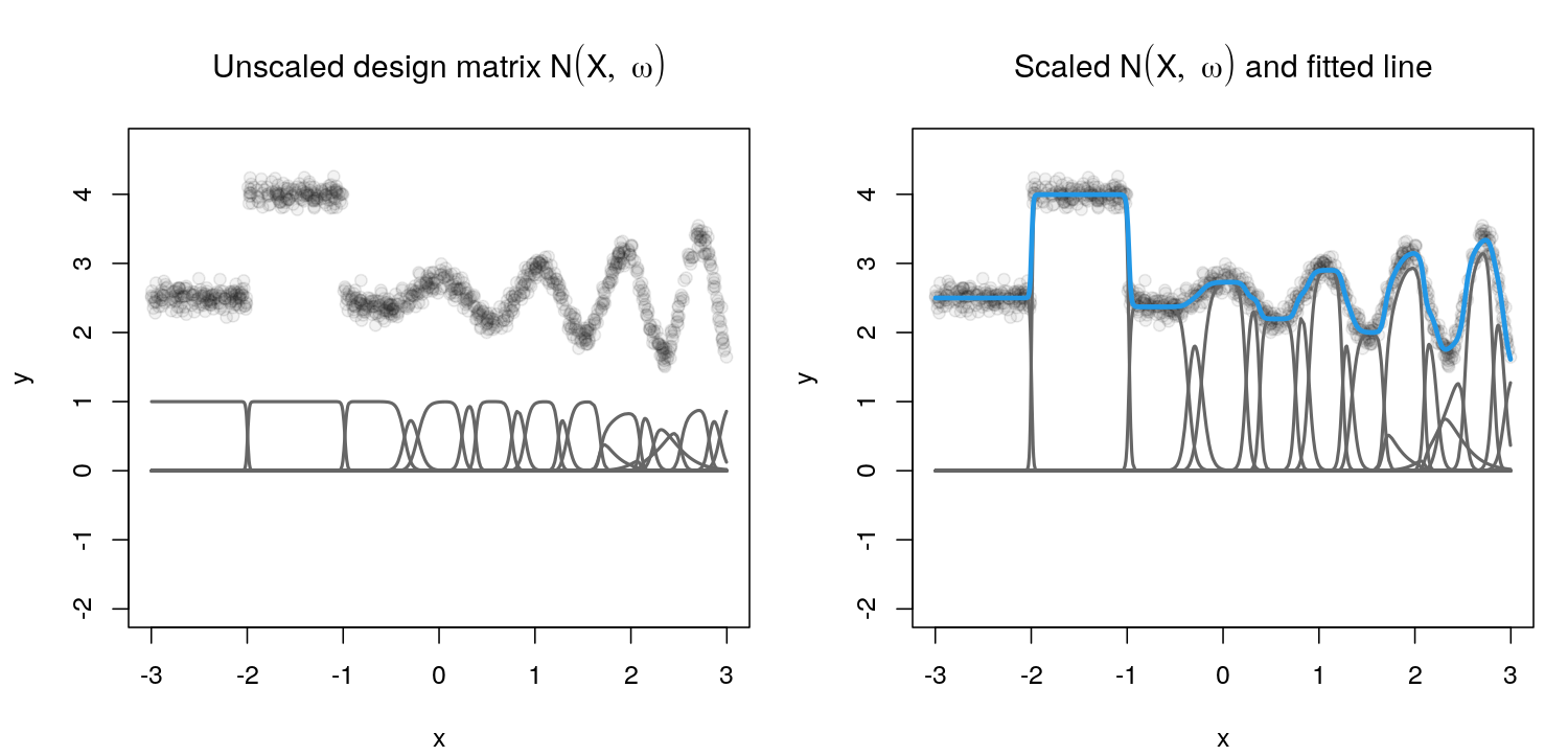
Figure 3: Learned design matrix $\text{\boldmath$N$}(\text{\boldmath$X$},\mathbf{\Omega})$ using an univariate SoRT and training data. The left plot depits the data (light-grey points) together with the unscaled basis functions (solid grey lines). The right plot shows the basis functions scaled with regression parameters $\boldsymbol{\beta}$ together with the fitted curve $\text{\boldmath$N$}(\text{\boldmath$X$},\mathbf{\Omega})\text{\boldmath$\beta$}$ (blue line).

This figure shows a step function with subsequent highly oscillatory relationship between $x$ and $y$. The example shows very well how a SoRT is suitable for both abrupt changes and smooth functional shapes. Moreover, the SoRT can be viewed as a method that learns basis functions, e.g., similar to B-spline basis functions used for P-splines (Eilers and Marx, 1996). The main difference to the latter is that the basis functions from a SoRT are adaptive and smooth and can model very complex relationships, while the number of terminal nodes (columns in the design matrix $\text{\boldmath$N$}(\text{\boldmath$X$},\mathbf{\Omega})$) is much less compared to the degrees of freedom that are needed to obtain a similar fit with (P)-splines. In this example, the tree only needs $T=20$ terminal nodes to approximate the training data quite well already and the corresponding spline model fitted with the R package mgcv (Wood, 2022) requires $\approx 156$ degrees of freedom.

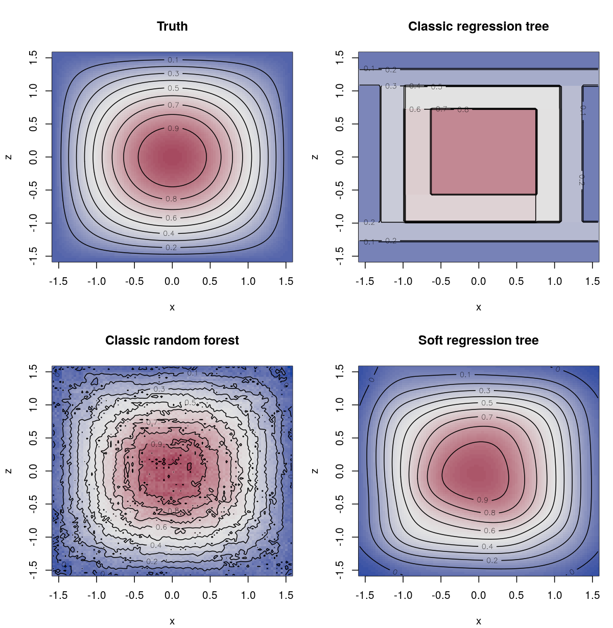
Figure 4: Artificial 2D data example. The true function is shown in the top left panel. The estimated function using a classic regression tree is shown in the top right panel, the estimated function using a RF with $2000$ trees is shown in the bottom left panel and the estimated function from the SoRT in the bottom right panel.

Another feature of the SoRT is its ability to model smooth interactions, such as those often found in spatial regression problems. An example is given in Figure 4. Here, the true function is given by $f(x,z)=\sin(x)\cdot\sin(z)$ and $10000$ data points are simulated using the Gaussian mean regression model $y_{i}=f(x_{i},z_{i})+\varepsilon_{i}$ with $\varepsilon_{i}\sim N(0,0.1^{2})$ and based on 100 equidistant values $x,z\in[-\pi/2,\pi/2]$ each. The true function $f$ is given in the upper left panel of Figure 4. The classical regression tree in the upper right panel shows that the true function can only be very roughly approximated, which is natural since the hard splits generated can only model rectangular regions. Therefore, to better capture complex interactions, a RF is estimated in many regression situations (Breiman, 2001). By growing several trees on data subsets and then aggregating over the trees to predict the response, a RF is also able to model almost smooth transitions. However, as can be seen in the lower left panel of Figure 4 even a RF with $2000$ trees is not able to reproduce the smooth surface of the true function very nicely, as the shown contour lines depict a rather rough estimate. In contrast, the SoRT with only 24 terminal nodes is able to reproduce the true functional form quite well (compare the lower right panel). What we have now illustrated for 1-2 dimensions only naturally extends to much higher dimensional interactions making a SoRT particularly attractive in many data situations.

Technically, the reason for the good approximation abilities is mainly the structural form of the SoRT, which is quite similar to a NN with a single hidden layer, which is known to be a universal function approximator (Hornik, 1991, and also Section 4.4). However, as mentioned earlier, the SoRT iteratively learns the shape of the design matrix $\text{\boldmath$N$}(\text{\boldmath$X$},\mathbf{\Omega})$ in multiple directions, whereas a NN with a single hidden layer is just a sum of scaled activation functions. In summary, the SoRT is a very flexible tool for modeling complex relationships, it can represent both soft transitions and step functions of a classical regression tree.

2.2 Adaptive Soft Regression Tree Predictor

We will extend the basic soft tree structure of the previous Subsection 2.1 to allow for more efficient and better predictions. For the moment keep in mind the example of a SoRT presented in Figure 2. The basic idea of growing a tree is that we only allow new nodes to emerge at positions where there is still a lot of unexplained information. E.g., in Figure 3, an additional soft split in the range $-3<x<-1$ would not improve the model fit much, since the first split could already approximate the step function behaviour quite well. Therefore, if there is a global functional shape that can be well approximated with a few splits then technically it will be better to maintain the model fit in that region of the data, rather than always computing new models that include all terminal nodes. This means that growing the SoRT should coarsely adapt to the global functional form at the beginning and only model fine-grained information in later steps as the tree grows. This behavior can be easily implemented by providing parameters to all $J=M+T$ nodes (except the root node) of the SoRT rather than just to the terminal leaf nodes as done for classical SoRT (Luo et al., 2021). To set this up, we do not only assign path probabilities of the form (4) to the terminal nodes but rather to all nodes and call this version “adaptive soft regression tree” (AdaSoRT). Let thus $D_{(l)}$ be any path from the root node to any node $N_{l}(\text{\boldmath$x$})$. Let also similar to before $\mathcal{D}_{(l)}$ be the set of nodes involved in forming in path $D_{(l)}$ of length $1\leq|\mathcal{D}_{(l)}|\leq\log_{2}(T)$, with path probability $P_{(l)}$ from (4) and set of weights $\mathbf{\Omega}_{(l)}$. With these probabilities we then define a feature-specific predictor of the form

$$\eta(\text{\boldmath$x$})=\beta_{0}+\sum_{j=1}^{J}P_{j}(\text{\boldmath$x$},\mathbf{\Omega}_{(j)})\beta_{j},$$ (5)

where $\beta_{0}$ is an overall intercept representing the root node. Hence, for instance for the tree in Figure 2, we obtain $J=6$ elements for the AdaSoRT or more generally $J=\sum_{l=1}^{\log_{2}(T)}2^{l}$. This tree structure thus allows us to decompose the predictor into coarse and fine elements, with the finer structures tending to be controlled by the rearmost elements of the sum of (5), i.e., the terminal nodes in Figure 2. The final AdaSoRT can again be represented by

$$\boldsymbol{\eta}=\text{\boldmath$N$}(\text{\boldmath$X$},\mathbf{\Omega})\text{\boldmath$\beta$},$$

but now with $1+M+T=1+J$ columns in the design matrix $\text{\boldmath$N$}(\cdot)$ (as opposed to $T$ columns for the classical SoRT), corresponding to the intercept and respective nodes that are generated in the growing steps and $\mathbf{\Omega}$ is now the set of the weights for all paths together.

3 AdaSoRT for Structured Additive Distributional Regression

SoRT introduced so far are able to efficiently make point predictions even when the underlying relation to covariates is rather complex or high-dimensional. With the extension AdaSoRT to the adaptive version of SoRT of the previous section, we can make estimation and accuracy of point predictions even more efficient. However, often predicting the conditional first moment of the quantity of interest (i.e., the expected value) is not enough. Rather, being able to infer complete predictive distributions and to derive further quantities from it (such as scale, prediction intervals, certain quantiles or tail measures) becomes more and more relevant in many modern applications (e.g., electricity price forecasting, Nowotarski and Weron, 2018 or climate change, Räisänen, 2022); including the empirical illustration in this paper on forecasting the Sun’s solar cycle 25 and 26 in Section 7. To address this task, we propose AdaSoRT for structured additive distributional regression – which we refer to as Distrubtional AdaSoRT (DAdaSoRT) and present how these flexible models can be fitted efficiently and how to perform model choice.

3.1 Model Specification

The idea of structured additive distributional regression (or GAMLSS; Rigby and Stasinopoulos, 2005; Klein et al., 2015a) is to model all parameters of an arbitrary parametric response distribution (rather than just the mean of an exponential family distribution) through available features. Specifically, assume

$$y\sim{{D}_{y}}\left(h_{1}(\theta_{1})=\eta_{1},\,\,h_{2}(\theta_{2})=\eta_{2},\dots,h_{K}(\theta_{K})=\eta_{K}\right),$$ (6)

where ${{D}_{y}}$ denotes a parametric distribution for the response variable $y$ (which can in our framework also be non-continous or multivariate; see e.g. Klein et al., 2015b, a) with $K$ parameters $\theta_{k}\equiv\theta_{k}(\text{\boldmath$x$})$, $k=1,\ldots,K$, that are linked to feature-dependent predictors $\eta_{k}\equiv\eta_{k}(\text{\boldmath$x$})$ using known monotonic and twice differentiable functions $h_{k}(\cdot)$. The latter are simply chosen to meet potential parameter space restrictions on $\theta_{k}$. The distribution $\mathcal{D}_{y}$ is arbitrary, but we assume it has a parametric probability density/mass function $f_{y}(\cdot;\theta_{1},\ldots,\theta_{k})$ and that this density is twice continuously differentiable with respect to all distributional predictors $\eta_{k}$.

Using the AdaSoRT presented in Section 2.2, the $k$-th predictor for distributional parameter $\theta_{k}$ is then given by

$$\boldsymbol{\eta}_{k}\equiv\eta_{k}(\text{\boldmath$X$}_{k};\boldsymbol{\beta}_{k},\mathbf{\Omega}_{k}) = \text{\boldmath$N$}_{k}(\text{\boldmath$X$}_{k},\mathbf{\Omega}_{k})\boldsymbol{\beta}_{k}$$ (7)

$$= \begin{pmatrix}1&P_{k,1}(\text{\boldmath$x$}_{k,1},\mathbf{\Omega}_{k})&\cdots&P_{k,J_{k}}(\text{\boldmath$x$}_{k,1},\mathbf{\Omega}_{k})\\ \vdots&\vdots&\ddots&\vdots\\ 1&P_{k,1}(\text{\boldmath$x$}_{nk},\mathbf{\Omega}_{k})&\cdots&P_{k,J_{k}}(\text{\boldmath$x$}_{nk},\mathbf{\Omega}_{k})\end{pmatrix}\begin{pmatrix}\beta_{k,0}\\ \beta_{k,1}\\ \vdots\\ \beta_{k,J_{k}}\end{pmatrix},$$

where the columns of $\text{\boldmath$N$}_{k}(\text{\boldmath$X$}_{k},\mathbf{\Omega}_{k})$ are similarly defined as in (4) but now each distributional parameter $\eta_{k}$ is learned from the data through an AdaSoRT with distribution parameter specific set of nodes $\mathcal{N}_{k}=\mathcal{M}_{k}\,\dot{\cup}\,\mathcal{T}_{k}$, $\mathcal{M}_{k}=M_{k}$, $\mathcal{T}_{k}=T_{k}$ with $J_{k}+1=M_{k}+T_{k}+1$ columns. Furthermore, $\mathbf{\Omega}_{k}$ is the set of weights associated with all paths of the $k$-th AdaSoRT and $\text{\boldmath$\beta$}_{k}=(\beta_{k,0},\beta_{k,1},\ldots,\beta_{k,J_{k}})^{\top}\in\text{$\mathds{R}$}^{J_{k}}$ are the unknown parameters. Finally, we remark that in principal, for each distributional parameter $\theta_{k}$ a different feature matrix $\text{\boldmath$X$}_{k}$ can be used. To detail likelihood-based estimation in the following, we write $\text{\boldmath$\beta$}=(\text{\boldmath$\beta$}_{1},\ldots,\text{\boldmath$\beta$}_{K})^{\top}$ and $\mathbf{\Omega}=(\mathbf{\Omega}_{1},\ldots,\mathbf{\Omega}_{K})^{\top}$ for the vectors of all unknown parameters.

3.2 Estimation

Next, we detail how estimation of the parameters $\boldsymbol{\beta}$ and $\omega$ of a DAdaSoRT can be performed. Assume having a trained data set $\{(\text{\boldmath$x$}_{i},y_{i})\}_{i=1,\ldots,n}$ of features $\text{\boldmath$x$}_{i}$ and outputs $y_{i}$ (w.l.o.g. we write down the case for univariate $y$). Let $\text{\boldmath$X$}_{k}=(\text{\boldmath$x$}_{1k}^{\top},\ldots,\text{\boldmath$x$}_{nk}^{\top})^{\top}$ for $k=1,\ldots,K$ be the feature matrix of $\theta_{k}$ and denote $\text{\boldmath$X$}=(\text{\boldmath$X$}_{1}^{\top},\ldots,\text{\boldmath$X$}_{K}^{\top})^{\top}$ or the complete feature matrix of all $K$ parameters and all $n$ data points. The loss function is induced by the log-density $f_{y}$ chosen by the user and reads as

$$\ell(\boldsymbol{\beta},\text{\boldmath$\omega$};\mathbf{y},\text{\boldmath$X$})=\sum_{i=1}^{n}\log\,f_{y}(y_{i};\theta_{i1}=h_{1}^{-1}(\eta_{1}(\text{\boldmath$x$}_{i1};\boldsymbol{\beta}_{1},\text{\boldmath$\omega$}_{1})),\ldots,\theta_{iK}=h_{K}^{-1}(\eta_{K}(\text{\boldmath$x$}_{iK};\boldsymbol{\beta}_{K},\text{\boldmath$\omega$}_{K}))).$$

Denoting $t=0,1,2,\ldots,$ the outer iteration index and $k=1,\ldots,K$ the distributional parameter, our algorithm then proceeds as follows:

1. Intialization of root nodes: First, the $K$ root nodes or intercepts $\beta_{0k}$ are initialized, i.e., intercept only models are applied and we set $\eta_{k}^{(0)}=\beta_{0k}$ for $k=1,\ldots,K$

2. Splitting the root nodes and efficient sub-indexing: Afterwards, the first soft split for each $k$-th parameter is calculated using the current score vector $\mathbf{u}_{k}=\partial\ell(\boldsymbol{\beta},\text{\boldmath$\omega$};\mathbf{y},\text{\boldmath$X$})/\partial\boldsymbol{\eta}_{k}$ and working weights
   $\mathbf{W}_{kk}=-\mathrm{diag}(\partial^{2}\ell(\boldsymbol{\beta},\text{\boldmath$\omega$};\mathbf{y},\text{\boldmath$X$})/\partial\boldsymbol{\eta}_{k}\partial\boldsymbol{\eta}_{k}^{\top})$. Assume for this that we have a set of optimal weights $\text{\boldmath$\omega$}_{k}=\{\text{\boldmath$\omega$}_{1k}\}$ (estimated by e.g. maximum likelihood), which determines the first split and results in the $n\times 2$ design matrices $\text{\boldmath$N$}_{1k}(\mathbf{X}_{k},\text{\boldmath$\omega$}_{k})$. At this point recall, that for one split only one vector of weights is needed. Next, we introduce the sub-index $c=1,\ldots,\frac{J_{k}}{2}$ and denote by $\text{\boldmath$N$}_{ck}(\cdot)$ the $n\times 2$ design matrices with two columns each, i.e. $\text{\boldmath$N$}_{k}(\mathbf{X}_{k},\text{\boldmath$\omega$}_{k})=(\mathbf{1},\text{\boldmath$N$}_{1k}(\mathbf{X}_{k},\text{\boldmath$\omega$}_{k}),\ldots,\text{\boldmath$N$}_{\frac{J_{k}}{2}k}(\mathbf{X}_{k},\text{\boldmath$\omega$}_{k}))$ for each $c$ and each $k$. Doing so, the estimation problem can be significantly simplified, since improving the model fit only requires $n\times 2$ matrices, matching the two-dimensional sub-vectors $\boldsymbol{\beta}_{ck}$ of $\boldsymbol{\beta}_{k}=(\beta_{0k},\boldsymbol{\beta}_{1k}^{\top},\ldots,\boldsymbol{\beta}_{\frac{J_{k}}{2}k}^{\top})^{\top}$. Now, given the first $n\times 2$ design matrices $\text{\boldmath$N$}_{1k}(\cdot)$, the predictor is updated by first solving

   $$\boldsymbol{\beta}_{1k}=(\text{\boldmath$N$}_{1k}(\text{\boldmath$X$}_{k},\text{\boldmath$\omega$}_{k})^{\top}\mathbf{W}_{kk}\text{\boldmath$N$}_{1k}(\text{\boldmath$X$}_{k},\text{\boldmath$\omega$}_{k})+\zeta\mathbf{I})^{-1}\text{\boldmath$N$}_{1k}(\text{\boldmath$X$}_{k},\text{\boldmath$\omega$}_{k})^{\top}\mathbf{u}_{k}$$ (8)

   and then setting $\boldsymbol{\eta}_{k}^{(t+1)}=\boldsymbol{\eta}_{k}^{(t)}+\text{\boldmath$N$}_{1k}(\text{\boldmath$X$}_{k},\text{\boldmath$\omega$}_{k})\boldsymbol{\beta}_{1k}$ (see, e.g., Umlauf et al., 2018), where in the first split $t=1$. Here, the matrix $\zeta\mathbf{I}$ is a ridge penalty matrix with very small values on the diagonal, e.g. $\zeta=0.00001$, which only should ensure numerical stability.

3. Building the trees: In the next step, each column of $\text{\boldmath$N$}_{k}(\text{\boldmath$X$}_{k},\text{\boldmath$\omega$}_{k})$ is doubled as in Step 2 when splitting the root node again assuming a set of weights that are now $\text{\boldmath$\omega$}_{k}=\{\text{\boldmath$\omega$}_{1k},\text{\boldmath$\omega$}_{2k},\text{\boldmath$\omega$}_{3k}\}$ for each $k$ (compare Figure 2). For each of the newly created design matrices, the parameters $\boldsymbol{\beta}_{2k}$ and $\boldsymbol{\beta}_{3k}$ are then calculated as in (8), but in contrast to Step 2 the predictors are not updated immediately. Instead, only the soft split in parameter $\theta_{k}$ that contributes the most to the log-likelihood is selected for updating. The same steps are performed for all distributional parameters $\theta_{k}$.

4. Updating the weights: Updating the weights $\text{\boldmath$\omega$}_{rk}$, $r=1,\ldots,S_{k}$, where $S_{k}$ is the number of weights at iteration $t$, only requires first and second order derivatives of the log-likelihood w.r.t. $\text{\boldmath$\omega$}_{rk}$, which by the chain rule is easy to derive analytically. The weight updates can efficiently be computed based on (8) using the current $\boldsymbol{\beta}_{ck}$. For instance, at iteration $t=1$, e.g. for the first split, $\text{\boldmath$\omega$}_{1k}$, is based on

   $$\text{ML}(\text{\boldmath$\omega$}_{rk}|\text{\boldmath$y$},\text{\boldmath$X$})=\underset{\text{\boldmath$\omega$}_{rk}}{\text{arg max }}\ell(\text{\boldmath$\omega$}_{rk};\text{\boldmath$y$},\text{\boldmath$X$}).$$

Overall, this algorithm successively improves the model fit by calculating a new soft split at the “best” position for each $\theta_{k}$, while cycling through Steps 3, 4 for $t=1,2,\ldots,$ until convergence has been reached. We define the latter to be the case when no improvement in terms of the AIC can be achieved by further increasing the trees, for which the degrees of freedom are determined by the number of parameters in $\boldsymbol{\beta}$.

4 Extensions and Properties

In this section we highlight useful extensions of DAdaSoRT and summarize selected properties.

4.1 Avoiding Overfitting

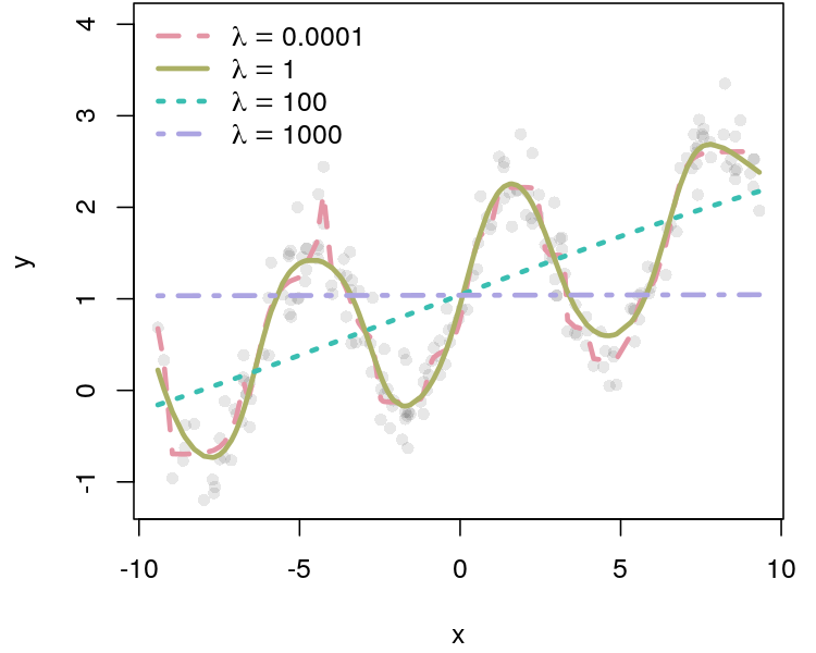
Figure 5: Avoiding overfitting. Shrinkage effect of $\lambda$ using simulated data.

When maximizing the weights $\text{\boldmath$\omega$}_{rk}$ an additional shrinkage penalty $\lambda_{k}J(\text{\boldmath$\omega$}_{rk})=\lambda_{k}\text{\boldmath$\omega$}_{rk}^{\top}\text{\boldmath$\omega$}_{rk}$ can be imposed to avoid overfitting. This yields the penalized maximum likelihood

$$\text{pen ML}(\text{\boldmath$\omega$}_{rk}|\text{\boldmath$y$},\text{\boldmath$X$})=\underset{\text{\boldmath$\omega$}_{rk}}{\text{arg max }}\ell(\text{\boldmath$\omega$}_{rk};\text{\boldmath$y$},\text{\boldmath$X$})-\lambda_{k}J(\text{\boldmath$\omega$}_{rk}).$$

The effect for different values of one shrinkage parameter $\lambda\equiv\lambda_{k}$ is shown if Figure 5. For very small values of $\lambda$ the estimated function contains abrupt jumps, e.g., at about $x=-4$. For larger values of $\lambda$ the fit gets smoother and smoother until a linear function is estimated and in the limit a simple constant functional form would be fitted. The selection of the shrinkage parameter is problem specific and is basically the only hyperparameter that needs to be tuned. In practice, we set $\lambda_{k}$ equal for all distributional parameters which usually results in very good global model fits and accurate predictive distributions. Moreover, the determination of $\lambda_{k}$ is relatively simple: First, $\lambda_{k}$ is set to a rather high value, so that the algorithm stops after a small number of iterations. Then $\lambda_{k}$ is decreased so that a steady state of the AIC or BIC can be achieved. The reason for this is that too small values of $\lambda_{k}$ force the estimation algorithm to add additional complexity to the estimated functions, see the jumps for $\lambda=0.0001$ in Figure 5, leading to overfitting of the final model. Overfitting is easily recognized by the fact that the AIC continues to decrease with only very small improvements in the penalized likelihood. Of course this is a heuristic approach, but in our experience it works very well, see the simulation Section 6 and the application Section 7.

4.2 Effect Decomposition and Subsumed Special Cases

Naturally, our DAdaSoRT allows for so-called effect decomposition of the predictors, which can be useful in the GAMLSS context (see, e.g., Kneib et al., 2019) for interpretational purposes. For our case of a DAdaSoRT it could for instance be of interest to disentangle high-dimensional interactions through the soft tree predictor to increase predictive accuracy, while being able to interpret low-dimensional effects on specific aspects of the predictive distributions. For this purpose, a structured part $\boldsymbol{\eta}_{k}^{\text{struct}}$ can be added to each predictor with

$$\boldsymbol{\eta}_{k} = \boldsymbol{\eta}_{k}^{\text{struct}}+\boldsymbol{\eta}_{k}^{\text{srt}}$$

$$= \mathbf{X}\boldsymbol{\gamma}_{k}+\boldsymbol{\eta}_{k}^{\text{srt}}$$

where predictor $\boldsymbol{\eta}_{k}^{\text{srt}}$ represents the AdaSoRT predictor and is given in (7); and $\mathbf{X}\boldsymbol{\gamma}_{k}$ are additional structured main effects (such as linear effects or smooth effects of univariate input features). In the simple case of linear effects only, i.e. $\boldsymbol{\eta}_{k}^{\text{struct}}\equiv\boldsymbol{\eta}_{k}^{\text{lin}}$, this representation corresponds to direct connectors for NN. However, more general representations

$$\boldsymbol{\eta}_{k}^{\text{struct}}=f_{1k}(\text{\boldmath$x$})+\ldots+f_{S_{k}k}(\text{\boldmath$x$}),$$

with $s=1,\ldots,S_{k}$ smooth effects of features, can be added to (7). The advantage of such an extension is the interpretability of the main effects, which is normally not given for classical trees, forests and NNs. Therefore, identifiability constraints should be enforced as suggested by Rügamer et al. (2021).

4.3 DAdaSo Forests

Our DAdaSoRT naturally extends to ensemble of trees as in classical random forests (e.g, by bagging Breiman, 1996; Yıldız et al., 2016), which we refer to as DAdaSo forests. We deliberately do not discuss the ensemble method very prominently, but focus on the already very good approximation properties of a single DAdaSoRT for brevity and readibility of our paper, but added them in both the simulation and the application sections. In the simulation Section 6, we found that DAdaSo forests have qualitatively similar or slightly better performance compared to a single DAdaSoRT for datasets of approximately 2000 observations and above. Below that, a single DAdaSoRT has slightly better performance, the reason for this is mainly due to the choice of the shrinkage parameter in combination with bagging for forests, which we intentionally did not tune separately to emphasize the simplicity of the approach.

4.4 Relation to Neural Network Universal Approximators

While it is is beyond the scope of the paper to rigorously investigate whether and in what sense soft trees are in general universal approximators, a valid starting point for future research can be the results on standard multilayer feedforward networks. For these, Hornik et al. (1989) showed that they are capable of approximating any Borel measureable function on finite dimensional spaces provided sufficiently many hidden units are available. While the soft trees do not have hidden units, the splits, tree-depth and ensemble estimates of single trees combined with our choice for the mappings in (2) are expected to allow for a similar degree of flexibility with respect to its capability to approximate arbitrary complex functions.

5 Software Implementation

DAdaSoRTs are implemented in the R package softtrees (Umlauf, 2022). The package supports all families as implemented in the R packags bamlss (Umlauf et al., 2022) and gamlss.dist (Stasinopoulos and Rigby, 2022). The softtrees package along all supplementary materials of this article is available on GitHub: URL https://github.com/freezenik/softtrees. Further examples on how fit DAdaSoRT along with code are provided in the manual pages of the package.

6 Simulation Study

In this section we provide empirical evidence of the efficacy of DAdaSoRT for several data generating processes compared to relevant competitors from the literature. To this end, we investigate the performance of DAdaSoRT with respect to bias using the root mean squared error ($\sqrt{\text{MSE}}$) of deviations from the true predictors $\eta_{k}$ (point accuracy), and overall predictive accuracy of predictive distributions used for probabilistic forecasting using proper scoring rules. Specifically, for continuous outputs we compute the continuous rank probability score (CRPS; Gneiting and Raftery, 2007), and discrete outputs the logarithmic score.

Simulation design. We simulate data sets of sizes $n=500,1000,5000,10000$ from three different distributions: the normal distribution (NO), the Gumbel distribution (GU) and the negative binomial distribution (NBI) from the R package gamlss.dist. The package uses a specific naming convention for the parameters of the distributions and supports up to four-parameter distributions. The parameters are $\mu$, $\sigma$, $\nu$ and $\tau$. In the simulation study, we let the parameters $\mu$ and $\sigma$ depend on feature vectors. Since all the distributions studied in this framework have two parameters, no specifications are required for $\nu$ and $\tau$. Specifically, we simulate data using

$$\eta_{\mu}=\left[\left(10\sin(\pi x_{1}x_{2})+20(x_{3}-0.5)^{2}+10x_{4}+5x_{5}\right)-1.5\right]\frac{2}{26.48}+1$$

for the predictor of parameter $\mu$ and

$$\eta_{\sigma}=\left(\left(z_{1}^{2}+\left(z_{2}z_{3}-\frac{1}{z_{2}z_{4}}\right)^{2}\right)^{0.5}-7.96\right)\frac{2}{1736.85}-2.5,$$

for $\sigma$ for all three data distributions. These predictors represent state-of-the art benchmark studies as the predictors are slightly scaled versions of the Friedman 1 and 2 functions (Friedman, 1991; Breiman, 1996). Following earlier work, the inputs $x_{1},\ldots,x_{5}$ and $z_{1},\ldots,z_{4}$ are drawn independently from uniform distributions with $x_{q}\sim U(0,1)$, $q=1,\ldots 4$, $z_{1}\sim U(0,100)$, $z_{2}\sim U(40,560\pi)$, $z_{3}\sim U(0,1)$ and $z_{4}\sim U(1,11)$. Finally, for each of the settings, we replicate the simulation $100$ times.

Benchmark methods. We compare the DAdaSoRT (denoted by srt) and the DAdaSo forests (denoted by srf) to a full Bayesian structured additive distributional regression model, estimated with the R package bamlss (denoted by bamlss) and distributional regression forests (Schlosser et al., 2019) as implemented in the R package disttree (Schlosser et al., 2021, denoted by distforest). Compared to srt representing a single tree, distforests are based on $1000$ trees each. For srf we use only $100$ trees due to computation time. For bamlss models, we use thin-plate splines (Wood, 2003) for nonlinear smooth effects, one for each covariate, estimated by Markov chain Monte Carlo simulation.

Results. Figure 6 summarizes results for all methods and metrics. To achieve direct comparability of results across the different settings, for each data distribution, we simulated one further test data set with $n=10000$ observations that was fixed throughout. Shown results are the median metric across the 100 replications.

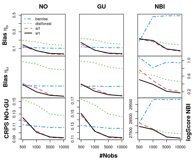
Figure 6: Simulation study. The first two rows show the deviation from the true and the estimated predictor (Bias $\eta_{k}$) measured my the median $\sqrt{\text{MSE}}$ over the $100$ replications for different number of training samples and data distributions; the normal (NO), Gumbel (GU) and negative binomial (NBI). The true predictors $\eta_{\mu},\eta_{\sigma}$ are slightly scaled versions of Friedman 1 and 2 functions. The $\sqrt{\text{MSE}}\text{s}$ are calculated using a fixed data set with $10000$ test samples. The bottom row shows the corresponding CRPS for NO and GU and the logarithmic score for NBI using the same test data.

Looking at the performance in terms of bias, CRPS and logarithmic scores, srt and srf clearly outperform the other methods. Only for very small data sets with $500$ observations the bamlss models show slightly better results for distribution NO and GU. Furthermore, srf is slightly better in all settings according the predictor for parameter $\mu$ and is slightly better according the CRPS and logarithmic score for $n>1000$. For $n\leq 1000$ srt is slightly better according the predictor for $\sigma$ for NO and GU and for all $n$ for NBI and also according to the logarithmic score for $500$ training points for NBI. The reason for this is that srf is computed using bagging and we did not adapt the shrinkage parameter separately to emphasize the simplicity of the approach, i.e., srf can most likely outperform more settings. Interestingly, the distforest seems to have the worst performance for the distributions NO and GU for all sizes of training data, i.e., the method apparently cannot find the non-linear structure of the simulated predictors very well. Only in the count data setting with $500$ and $1000$ training points the results of the logarithmic score for distforest are very similar to srt and srf.

Conclusion. In summary, it can be clearly identified that srt and srf are very well suited to finding non-linear relationships in the data compared to the conventional distforest. As expected, the bamlss models cannot approximate the non-linear structures very well. In contrast, both DAdaSoRT and DAdaSo forests are very robust across settings and are an attractive alternative to the considered benchmark methods in particular with large data and complex relations between outputs and inputs. The results for distforest and bamlss were calculated with the defaults of the software packages, only the number of trees was increased from 500 to 1000 for the distforests. The defaults for distforest are set so that very flexible structures can be found in principle. The only tuning parameter for DAdaSoRT is the shrinkage penalty for the weights, see Section 3.2, for which we have simply identified reasonably good values with the strategy as described in Section 4.1, meaning that further tuning could even improve the results, especially for the DAdaSo forests.

7 Solar Cycle Forecasting

The Sun’s activity has been closely observed and recorded for a very long time. The solar activity is determined by numerous explosions, also known as coronal mass ejections and solar flares, which emit a tremendous amount of energy. Solar flares emit X-rays and magnetic fields that can literally bombard earth as geomagnetic storms and thus affect activity on earth (see, e.g.; Hathaway, 2015). For instance, strong solar activity can change polarity of satellites and damage its electronics. Typically, these eruptions occur near sunspots, i.e., the more sunspots visible on the solar surface, the greater the solar activity. The number of sunspots follows a certain periodicity with a cycle of about eleven years. Therefore, the number of sunspots and the prediction of solar cycles are of particular interest and have thus been recorded since 1749. In the past decades, various models have been developed to forecast the number of sunspots. For example, in one of the most recent articles on sunspots at the time of writing (Dang et al., 2022), non-deep learning methods are compared with deep ensemble learning methods for prediction. The National Aeronautics and Space Administration (NASA) solar cycle forecast is available at https://www.nasa.gov/msfcsolar/ (last viewed on 2022/08/11) from the Space Environments Team in the Natural Environments Branch of the Engineering Directorate at Marshall Space Flight Center (MSFC). According to MSFC, monthly smoothed sunspot series are used to construct forecasts based on a regression model estimating the deviation from a mean solar cycle, also called MSFC solar activity future estimation (MSAFE) model (Suggs, 2017). The model is updated monthly, and the first published forecasts began in March 1999, and to our knowledge the model has not been changed since then.

In most studies, the different methods are typically compared using point estimates and then evaluated using, e.g., the MSE. To contribute to the topic of sunspot forecasting we use our proposed srt from Section 3.2) and benchmark it against point forecasts from the NASA’s MSAFE model (NASA) and the distributional regression forest (distforest) using the MSE. In addition, unlike other studies, we assess the full probabilistic predictive ability for srt and distforest using the CRPS score.

Our analysis is based on monthly mean sunspot data from November 1833 to June 2022 for the response $y_{t}$ with $t=1,\ldots,2263$, which is provided by SILSO World Data Center (1833-2022).

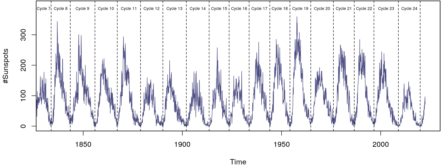
Figure 7: Solar cylce forecasting. Monthly mean sunspot data from November 1833 to June 2022.

The data $y_{t}$ is shown in Figure 7. To evaluate forecast performance, we use all 277 available NASA forecasts, with the first forecast starting in March 1999 and the last in September 2021, and compare them to the forecasts obtained by srt and distforest. For training we only use data before the respective NASA forecast starts. More precisely, we use lagged data of sunspot numbers as inputs for srt and distforest (24 monthly lags, $y_{t-1},y_{t-2},\ldots,y_{t-24}$, plus annual lags up to 35 years into the past, $y_{t-12\cdot j}$, $j=3,\ldots,35$) and compute predictions by recursive multi-step forecasting (see, e.g.; Ben Taieb and Hyndman, 2014). We additionally transform the response with $\tilde{y}_{t}=\sqrt{y_{t}+0.001}$ to achieve better numerical stability. In total, we use three different distributions (implemented in gamlss.dist) for comparison, the normal distribution (NO), the gamma distribution (GA) and the t family distribution (TF).

Because of the lagged input data structure, the choice of the shrinkage parameter $\lambda$ used in srt is more likely to influence the model performance, more than in usual regression settings. Therefore, we tested srt with $\boldsymbol{\lambda}=(1,5,10,50,100,500,1000)^{\top}$ and used the shrinkage parameter with the best forecast performance. In this way we manage to get a sense of different shrinkage and forecast horizons, the shortest horizon being nine months and the longest to date 236 months. For a detailed analysis, we evaluated short, medium and long forecast horizons (0 to 99 months, 100 to 199 months and $\geq$ 200 months, respectively).

	Horizon	1st	2nd	3rd
CRPS	short	srt-TF: 0.7835	srt-NO: 0.7870	srt-GA: 0.8678
	medium	srt-NO: 0.9325	srt-GA: 0.9679	srt-TF: 0.9739
	long	srt-GA: 1.0620	distforest-GA: 1.0700	distforest-TF: 1.0710
MSE	short	srt-NO: 147.50	srt-TF: 150.80	NASA: 288.50
	medium	srt-GA: 409.50	srt-NO: 435.70	distforest-TF: 439.80
	long	srt-GA: 562.50	distforest-GA: 590.90	distforest-NO: 626.80

Table 1: Solar cycle forecasting. Median CRPS and MSE scores for different forecast horizons, models and distributions, second and third best, column 1st, 2nd and 3rd respectively.

The results are shown in Table 1 and indicate that our proposed srt method outperforms distforest and also the forecast from NASA over all forecast horizons. The choice of the best distribution changes with the length of the forecast horizon indicating that full probabilistic models have advantages compared to models for the mean only. In particular, for long-term forecasts, srt in combination with the GA distribution seems to significantly improve the prediction quality compared to distforest and NASA, according to the reported metrics.

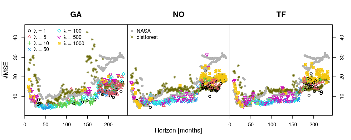
Figure 8: Solar cylce forecasting. Shown are the median $\sqrt{\text{MSE}}$s (y-axis) across the forecast horizons in months (x-axis) for the NO (left), GA (middle) and TF (right) distributions. The different colors and shapes correspond to the different values for $\lambda$. In addition, corresponding MSEs from NASA and distforest are indicated by the gray filled dots and olive asterix, respectively.

In Figure 8 the results for MSEs over the different forecast horizons are shown in more detail and illustrates that the srt method has a very good performance, especially for long term forecasts. Only for very short forecasts, up to 25 months, NASA seems to be slightly superior compared to srt. Overall, distforest performs worst in particular for short-term predictions. Note that the best distribution for srt, GA, is leading to very high values in the MSEs for distforest, while srt shows a stable performance for all distributions. In addition, Figure 8 shows that the choice of $\lambda$ for srt for long-term forecasts using the best-performing GA distribution consistently tends toward rather small values, implying a higher degree of model input interactions, and higher values with less interaction for short-term forecasts.

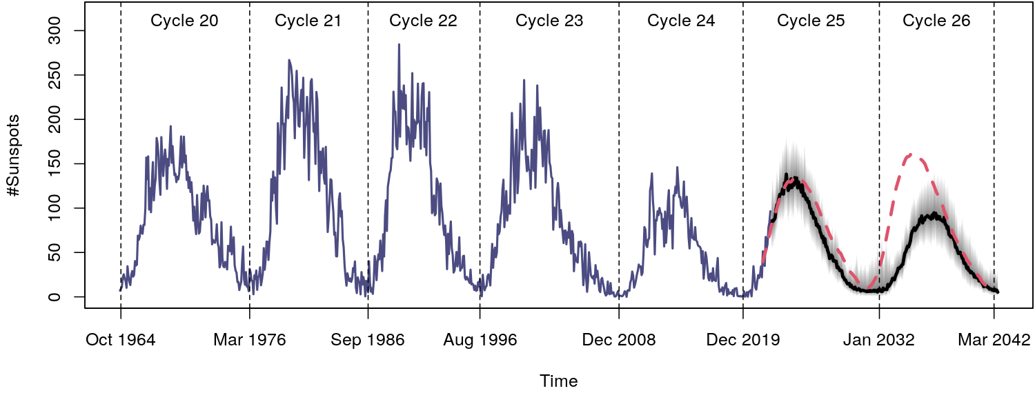
Figure 9: Solar cycle forecasting. Shown are monthly sunspot observations (dark blue lines) together with forecasts for solar cycle 25 and 26. The black line represents forecasts from the ensemble of 2000 srt trees with the GA distribution including 5% and 95% prediction intervals shown by the gray shaded area. The red dashed line represents the forecast from NASA.

As commonly the long term forecasts get the most attention, we finally estimate a model with all available data to try to predict the solar cycle 25 and 26, which corresponds to a long forecast of 242 months. To further minimize the uncertainties of the forecast we create a DAdaSo forest, srf, for the GA distribution. To do so, we train a total of 2000 srt trees on 63% of the data (bagging) and with $\lambda=2$ for each tree. The final ensemble forecast for solar cycle 25 and 26 is shown in Figure 9. It can be seen that the prediction for solar cycle 25 is essentially the same as provided by NASA, which consolidates the fact that NASA’s prediction could more or less come true in this way. For solar cycle 26 the differences in amplitude are clear, the srf predicts a much weaker cycle than NASA, while the predicted cycle of srf starts later. The shown prediction intervals of srf show a larger uncertainty especially in the maximum of the cycles and further illustrate the large difference in the forecast for solar cycle 26. At first sight, the shape of our predicted cycle 26 seems rather unrealistic compared to NASA’s forecast, but on closer inspection, solar cycles 7, 12, 13 and 14 (and earlier 5 and 6, not shown in Figure 7) are quite similar to our prediction.

To conclude, the proposed srt and srf can be seen as competitive methods for sunspot prediction. Especially the fact that with srt a full probabilistic forecast can be computed includes significant advantages for estimating the forecast uncertainty compared to point predictions. The predictive performance of the computed long-term forecast will be seen in the future, but we believe that srt and srf can certainly be a good alternative, although of course more work needs to done for better model specification and the definition of the hyperparameters.

8 Summary

In this paper, we developed SoRT for the distributional learning setting and proposed a number of extensions, including ensembles of DAdaSoRT. DAdaSoRT are a very flexible class of models that can be used for full probabilistic forecasting. For efficient estimation we present an adaptive algorithm, where the size of the SoRT is determined by information criteria such as AIC or BIC, leading to models with relatively few degrees of freedom. We show in an extensive simulation study that the performance of DAdaSoRT is better than, or at least similar to, that of a distributional random forest. The simulation results are also reflected in the solar activity prediction application. In summary, the proposed distributional adaptive soft regression tree (DAdaSoRT) is very competitive, especially in cases with a high degree of interactions amongst input features. However, in future research, some improvements need to be made in terms of algorithmic performance when using large datasets as well as the discussed extensions by decomposing the predictor into main and interaction effects. In addition, the question of the (universal) approximation capabilities remains open. We also plan to extend DAdaSoRT in the Bayesian context to obtain full Bayesian inference.

References

- Ben Taieb and Hyndman (2014) Ben Taieb S, Hyndman R (2014). “Boosting Multi-Step Autoregressive Forecasts.” In EP Xing, T Jebara (eds.), Proceedings of the 31st International Conference on Machine Learning, volume 32 of Proceedings of Machine Learning Research, pp. 109–117. PMLR, Bejing, China. URL https://proceedings.mlr.press/v32/taieb14.html.
- Breiman (1996) Breiman L (1996). “Bagging Predictors.” Machine Learning, 24, 123–140. 10.1023/A:1018054314350.
- Breiman (2001) Breiman L (2001). “Random Forests.” Machine Learning, 5, 5–32. https://doi.org/10.1023/A:1010933404324.
- Ciampi et al. (2002) Ciampi A, Couturier A, Li S (2002). “Prediction Trees with Soft Nodes for Binary Outcomes.” Statistics in Medicine, 21(8), 1145–1165. https://doi.org/10.1002/sim.1106.
- Consortium (2020) Consortium R (2020). “Estimating COVID-19 Trends using GAMLSS.” Https://www.r-consortium.org/blog/2020/12/17/estimating-covid-19-trends-using-gamlss.
- Dang et al. (2022) Dang Y, Chen Z, Li H, Shu H (2022). “A Comparative Study of non-deep Learning, Deep Learning, and Ensemble Learning Methods for Sunspot Number Prediction.” Applied Artificial Intelligence, 36(1), 2074129. 10.1080/08839514.2022.2074129.
- Eilers and Marx (1996) Eilers PHC, Marx BD (1996). “Flexible Smoothing Using B-Splines and Penalized Likelihood.” Statistical Science, 11, 89–121. 10.1214/ss/1038425655.
- Fahrmeir et al. (2013) Fahrmeir L, Kneib T, Lang S, Marx B (2013). Regression – Models, Methods and Applications. Springer-Verlag, Berlin.
- Friedman (1991) Friedman JH (1991). “Multivariate Adaptive Regression Splines.” The Annals of Statistics, 19(1), 1–67. 10.1214/aos/1176347963.
- Frosst and Hinton (2017) Frosst N, Hinton G (2017). “Distilling a Neural Network Into a Soft Decision Tree.” arXiv:1711.09784.
- Gneiting and Raftery (2007) Gneiting T, Raftery AE (2007). “Strictly Proper Scoring Rules, Prediction, and Estimation.” Journal of the American Statistical Association, 102(477), 359–378. 10.1198/016214506000001437.
- Hastie and Tibshirani (1990) Hastie T, Tibshirani R (1990). Generalized Additive Models. Chapman & Hall/CRC, New York.
- Hathaway (2015) Hathaway DH (2015). “The Solar Cycle.” Living Reviews in Solar Physics, 4(12), 1614–4961. 10.1007/lrsp-2015-4.
- Hornik (1991) Hornik K (1991). “Approximation capabilities of multilayer feedforward networks.” Neural Networks, 4(2), 251–257. https://doi.org/10.1016/0893-6080(91)90009-T.
- Hornik et al. (1989) Hornik K, Stinchcombe M, White H (1989). “Multilayer Feedforward Networks are Universal Approximators.” Neural Networks, 2(5), 359–366. https://doi.org/10.1016/0893-6080(89)90020-8.
- Hothorn et al. (2006) Hothorn T, Hornik K, Zeileis A (2006). “Unbiased Recursive Partitioning: A Conditional Inference Framework.” Journal of Computational and Graphical Statistics, 15(3), 651–674. 10.1198/106186006X133933.
- Irsoy et al. (2012) Irsoy O, Yildiz OT, Alpaydin E (2012). “Soft Decision Trees.” In Proceedings of the 21st International Conference on Pattern Recognition (ICPR2012), pp. 1819–1822.
- Klein et al. (2014) Klein N, Denuit M, Lang S, Kneib T (2014). “Nonlife Ratemaking and Risk Management with Bayesian Generalized Additive Models for Location, Scale, and Shape.” Insurance: Mathematics and Economics, 55, 225 – 249. 10.1016/j.insmatheco.2014.02.001.
- Klein et al. (2015a) Klein N, Kneib T, Klasen S, Lang S (2015a). “Bayesian Structured Additive Distributional Regression for Multivariate Responses.” Journal of the Royal Statistical Society C, 64, 569–591. 10.1111/rssc.12090.
- Klein et al. (2015b) Klein N, Kneib T, Lang S (2015b). “Bayesian Generalized Additive Models for Location, Scale and Shape for Zero-Inflated and Overdispersed Count Data.” Journal of the American Statistical Association, 110(509), 405–419. 10.1080/01621459.2014.912955.
- Kneib et al. (2019) Kneib T, Klein N, Lang S, Umlauf N (2019). “Modular Regression – A Lego System for Building Structured Additive Distributional Regression Models with Tensor Product Interactions.” TEST, 28(1), 1–39. 10.1007/s11749-019-00631-z.
- Kneib et al. (2021) Kneib T, Silbersdorff A, Säfken B (2021). “Rage Against the Mean – A Review of Distributional Regression Approaches.” Econometrics and Statistics. https://doi.org/10.1016/j.ecosta.2021.07.006.
- Linero and Yang (2018) Linero AR, Yang Y (2018). “Bayesian regression tree ensembles that adapt to smoothness and sparsity.” Journal of the Royal Statistical Society: Series B (Statistical Methodology), 80(5), 1087–1110. https://doi.org/10.1111/rssb.12293.
- Luo et al. (2021) Luo H, Cheng F, Yu H, Yi Y (2021). “SDTR: Soft Decision Tree Regressor for Tabular Data.” IEEE Access, 9, 55999–56011. 10.1109/ACCESS.2021.3070575.
- Nguyen (2002) Nguyen HS (2002). “A Soft Decision Tree.” In MA Kłopotek, ST Wierzchoń, M Michalewicz (eds.), Intelligent Information Systems 2002, pp. 57–66. Physica-Verlag HD, Heidelberg. ISBN 978-3-7908-1777-5.
- Nowotarski and Weron (2018) Nowotarski J, Weron R (2018). “Recent Advances in Electricity Price Forecasting: A Review of Probabilistic Forecasting.” Renewable and Sustainable Energy Reviews, 81, 1548–1568. https://doi.org/10.1016/j.rser.2017.05.234.
- Probst and Boulesteix (2018) Probst P, Boulesteix AL (2018). “To Tune or Not to Tune the Number of Trees in Random Forest.” Journal of Machine Learning Research, 18(181), 1–18. URL http://jmlr.org/papers/v18/17-269.html.
- Rigby and Stasinopoulos (2005) Rigby RA, Stasinopoulos DM (2005). “Generalized Additive Models for Location, Scale and Shape.” Journal of the Royal Statistical Society C, 54(3), 507–554. 10.1111/j.1467-9876.2005.00510.x.
- Rügamer et al. (2021) Rügamer D, Kolb C, Klein N (2021). “Semi-Structured Deep Distributional Regression: Combining Structured Additive Models and Deep Learning.” 2002.05777v4.
- Räisänen (2022) Räisänen J (2022). “Probabilistic Forecasts of Near-Term Climate Change: Verification for Temperature and Precipitation Changes from Years 1971–2000 to 2011–2020.” Climate Dynamics, 59(3), 1175–1188. 10.1007/s00382-022-06182-8.
- Schlosser et al. (2019) Schlosser L, Hothorn T, Stauffer R, Zeileis A (2019). “Distributional Regression Forests for Probabilistic Precipitation Forecasting in Complex Terrain.” The Annals of Applied Statistics, 13(3), 1564–1589. 10.1214/19-AOAS1247.
- Schlosser et al. (2021) Schlosser L, Lang MN, Hothorn T, Zeileis A (2021). \pkgdisttree: Trees and Forests for Distributional Regression. R package version 0.2-0.
- Serinaldi (2011) Serinaldi F (2011). “Distributional modeling and short-term forecasting of electricity prices by Generalized Additive Models for Location, Scale and Shape.” Energy Economics, 33(6), 1216–1226. https://doi.org/10.1016/j.eneco.2011.05.001.
- SILSO World Data Center (1833-2022) SILSO World Data Center (1833-2022). “The International Sunspot Number.” International Sunspot Number Monthly Bulletin and online catalogue. URL http://www.sidc.be/silso/.
- Simon et al. (2018) Simon T, Fabsic P, Mayr GJ, Umlauf N, Zeileis A (2018). “Probabilistic Forecasting of Thunderstorms in the Eastern Alps.” Monthly Weather Review, 146, 2999–3009. 10.1175/MWR-D-17-0366.1.
- Simon et al. (2019) Simon T, Mayr GJ, Umlauf N, Zeileis A (2019). “NWP-Based Lightning Prediction Using Flexible Count Data Regression.” Advances in Statistical Climatology, Meteorology and Oceanography, 5(1), 1–16. 10.5194/ascmo-5-1-2019.
- Stasinopoulos and Rigby (2022) Stasinopoulos DM, Rigby RA (2022). \pkggamlss.dist: Distributions for Generalized Additive Models for Location, Scale and Shape. R package version 6.0-5, URL https://CRAN.R-project.org/package=gamlss.dist.
- Suggs (2017) Suggs RJ (2017). “The MSFC Solar Activity Future Estimation (MSAFE) Model.” Https://ntrs.nasa.gov/citations/20170008081.
- Umlauf (2022) Umlauf N (2022). \pkgsofttrees: Soft Distributional Regression Trees and Forests. R package version 1.0, URL https://github.com/freezenik/softtrees.
- Umlauf et al. (2018) Umlauf N, Klein N, Zeileis A (2018). “BAMLSS: Bayesian Additive Models for Location, Scale, and Shape (and Beyond).” Journal of Computational and Graphical Statistics, 27(3), 612–627. 10.1080/10618600.2017.1407325.
- Umlauf et al. (2022) Umlauf N, Klein N, Zeileis A, Simon T (2022). \pkgbamlss: Bayesian Additive Models for Location, Scale, and Shape (and Beyond). R package version 1.1-8, URL http://www.bamlss.org/.
- Wood (2003) Wood SN (2003). “Thin plate regression splines.” Journal of the Royal Statistical Society: Series B (Statistical Methodology), 65(1), 95–114. https://doi.org/10.1111/1467-9868.00374.
- Wood (2017) Wood SN (2017). Generalized Additive Models : An Introduction with R. 2nd edition. Chapman & Hall/CRC.
- Wood (2022) Wood SN (2022). \pkgmgcv: Mixed GAM Computation Vehicle with Automatic Smoothness Estimation. R package version 1.8-40, URL https://CRAN.R-project.org/package=mgcv.
- Yıldız et al. (2016) Yıldız OT, İrsoy O, Alpaydın E (2016). “Bagging Soft Decision Trees.” In Machine Learning for Health Informatics: State-of-the-Art and Future Challenges, pp. 25–36. Springer International Publishing. 10.1007/978-3-319-50478-0_2.
- Ziel (2021) Ziel F (2021). “M5 competition uncertainty: Overdispersion, distributional forecasting, GAMLSS, and beyond.” International Journal of Forecasting. https://doi.org/10.1016/j.ijforecast.2021.09.008.