Virtual Screening on FPGA: Performance and Energy versus Effort

Abstract

With their wide-spread availability, FPGA-based accelerators cards have become an alternative to GPUs and CPUs to accelerate computing in applications with certain requirements (like energy efficiency) or properties (like fixed-point computations). In this paper we show results and experiences from mapping an industrial application used for drug discovery on several types of accelerators. We especially highlight the effort versus benefit of FPGAs compared to CPUs and GPUs in terms of performance and energy efficiency. For this application, even with extensive use of FPGA-specific features, and performing different optimizations, results on GPUs are still better, both in terms of energy and performance.

1 Introduction

Today FPGAs are proposed as an alternative to GPUs or CPUs to speed-up computation. They are available in the datacenter [17], and supercomputers are being build with FPGAs as their main compute elements [9]

With their massive parallelism, high-Bandwidth memory [6] and low energy consumption [5], they have clear benefits in certain situations to CPUs and GPUs. Also, in recent years, FPGA floating point performance has improved [4] and fixed point performance is even better.

While in the past you could only program FPGAs in low-level hardware description languages like Verilog or VHDL, these days using high-level programming in C or C++ and OpenCL is the norm. Indeed, high-level synthesis (HLS) tools have improved dramatically over the last years [10], and the use of so-called pragma’s allows a cleaner separation of pure functionality and FPGA-specific optimizations. Furthermore, both Intel and Xilinx have made their tools available without requiring a license, and have invested heavily in libraries to accelerate common compute tasks on FPGA (Intel oneAPI [1] and Xilinx Vitis [2]).

It has never been easier to get your first kernel running on an FPGA accelerator card. But do you get good performance and low energy consumption for compute-intensive applications? And how much time do you need to invest to optimize your code? How do these metrics compare to GPU and CPU implementations? In this paper we try to answer these questions studying a Virtual Molecule Screening (VMS) application.

This paper is organized as follows. In Section 2 we look at related work in FPGA mapping and performance optimizations. Section 3 introduces the VMS applications, which is optimized in Section 4. In Section 5, we look at performance numbers on FPGA and compare those to equivalent GPU and CPU versions. Sections 6 are the conclusions.

2 Related Work

High-Level Synthesis (HLS) has improved so much over the last year that it has become the de facto standard for FPGA acceleration [10]. HLS avoids the writing and verification of the functionality in low-level Hardware Description Language (HDL) like VHDL or Verilog. Yet it is known that such low-level HDL code can be fine-tuned for the FPGA resulting in much higher clock frequency, much better resource utilization and thus much better performance [19].

Alternatively, in the domain of machine learning, many frameworks exits to automatically generate HLS code, with optimizations for FPGA included [15]. Such frameworks are typically tuned to a specific subdomain, for example convolutional neural networks [14].

Older publications evaluating the mapping and optimization of compute-intensive kernels on FPGA show a clear energy advantage compared to GPU and CPU implementations [5]. Recently with the advent of larger GPUs and CPUs, FPGA only seem to excel in latency and seem outperformed by GPUs both in energy efficiency and performance [16]. Loop transformations have always played a crucial role in optimizing HLS code [12].

3 Virtual Molecule Screening

In this section we explain some key characteristics of the Virtual Molecule Screening application.

3.1 Chemogenomics and Matrix Factorization

In chemogenomics the key problem is the identification of candidate molecules that affect proteins associated with diseases. If this is done using machine learning techniques, the process is called compound-activity prediction [13]. Bayesian Matrix Factorization (BMF [11]) is a technique borrowed from recommender systems that has been successfully used for compound activity prediction. Thanks to the Bayesian approach, BPMF has been proven to be more robust to data-overfitting and Gibbs sampling makes the models feasible to compute. Another benefit, compared to for example deep learning, is that predictions from BMF models include confidence estimation, that can be used as a quality metric.

3.2 Virtual Screening

Once the models have been built, drug companies want to use them to evaluate millions of molecules in so-called virtual screens. Figure 1 shows a simplified view on the prediction flow for activity prediction. A molecule represented by its chemical fingerprint is fed in on the left. From the fingerprint an internal latent representation is computed, and this latent representation is used to make predictions on one or more protein targets. The amount of computation depends on the number of molecules, the number of Gibbs samples, the size of the latent representation and the number of protein targets. Since many compounds need to be tested, virtual screening requires much computational power, justifying the need for acceleration.

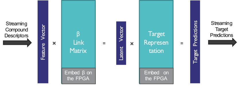
Figure 1: Virtual Molecule Screening (VMS) Pipeline

3.3 Virtual Screening Kernel

The main part of the VMS application is its kernel. More than 90% of the runtime is spent in this part of the application. To prepare for acceleration we have rewritten the kernel in HLS-ready C++. We have wrapped it in an OpenCL interface, to make it suitable for offloading.

4 Accelerating VMS using FPGAs

As already discussed in Section 2, there are clear benefits and challenges related to FPGAs. In this section we describe the different steps to exploit, avoid or remedy these benefits and challenges, by optimizing and rewriting our VMS application. In the next section we refer back to these steps when we evaluate performance, energy efficiency and optimization effort.

The steps are present here from most generic optimization, towards most targeted towards the actual FPGA device and the prediction model used. This order happens to coincide with going from the inner parts of the kernel, the lowest level of optimizations (the operations), over the loops, and functions of the kernel, outwards to the kernel as a whole and even beyond the kernel to the host interface.

4.1 Code Complexity

Mapping code efficiently on FPGA is a time-consuming task, even with help of high-level synthesis tools. Luckily for us, the VMS application code base is small and simple.

The structure of the kernel is a set of nested for loops. We have applied loop blocking [7]. By carefully choosing the block-size, we can fine-tune the kernel parallelism to match the available resources of the FPGA.

4.2 Bit-Width Reduction

FPGAs deal much better with reduced bit-width fixed point numbers than with double or single floating point numbers [4]. We were able to reduce the bit width of the input and output streams, and of the model itself from 64 bit floating point to 16bit and 8bit fixed point, without a significant loss in prediction accuracy. We did this using profiling and automatic fixed point refinement [8].

4.3 Parallelism

Compared to CPUs, FPGAs have a clock-speed that is 10x lower than CPUs. They compensate for this by providing many more parallel resources (DSP blocks, memory’s, LUTs, …). We were able to benefit from these extra resources by exploiting parallelism at many levels: inside the prediction pipeline, but also across proteins and molecules.

The use of Xilinx HLS pragmas allowed use to perform these optimizations unobtrusively, and allowed us to explore many ways to exploit the parallelism, at loop level (using loop unrolling, and loop pipelining), and at the function level using dataflow parallelism with FPGA-based state machines.

Since compute now happens distributed, data needs to be distributed as well. Data distribution mirrors the loop transformations and is implemented using the pragma array partition. The data distribution for the dataflow across functions is implemented using HLS streams.

4.4 Memory Bandwidth

As with all accelerators, getting data in and out efficiently is key to good performance. In this case we achieved this by streaming the fingerprints in and predictions out linearly, and by storing the model itself in the FPGA on-chip memory beforehand.

Streaming was implemented by fine-tuning the AXI interface to the kernel. This allowed us to do AXI pipelined burst accesses and use the full bitwidth (512bits) of the memory interface.

4.5 Kernel Dimensions

To make most efficient use of the FPGA resources we have to make sure the kernel matches the amount of each of them available. We can influence this by changing the kernel dimensions, for example, by choosing how many compounds, or samples we process in parallel. We have also optimized the number of compounds per kernel invocation to reduce the kernel invocation overhead, and increase the efficiency of the dataflow and loop pipelining.

4.6 Kernel Interface

The final step is outside the kernel itself, at the level of the OpenCL interface. This involves instantiating multiple instances of the kernel to make optimal use multiple regions on the FPGA (SLRs [18]), each with their own DRAM memory interface.

We also make sure to overlap communication and computation at this level by using asynchronous OpenCL call [21].

5 Results and Discussion

In this section we evaluate the different optimization steps, we compare the final results to a GPU and CPU implementation and discuss performance versus effort for the three implementations.

5.1 Optimization Steps

We evaluated the aforementioned optimization steps on a Xilinx Alveo U200 [20] datacenter card on the VMS application. Figure 2 shows the effect of each of the step on performance and resource usage. Both are calculated as a percentage of peak based on the number of available DSP slices. Noting that the Y-axis is logarithmic, each step increased the performance with a factor, indicated on each point in the graph. The total performance increases with a factor $1351\times$ and the total resource usage with $280\times$, indicating the crucial importance of optimizing the generated C++ code.

The highest improvement comes from the step that tunes the kernel dimensions because that step enables the full parallelism of the FPGA. While the steps preceding this step also have a significant positive effect on performance, they are also important enabler steps to Kernel Dimensions step. They increase the effect of this step.

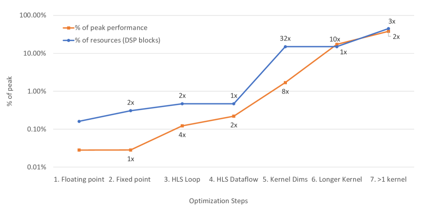
Figure 2: Effect of the Different optimization steps on performance (as a percentage of peak performance) and on resource usage (as a percentage of DSP blocks used)

5.2 Comparison

Two alternative implementations were of VMS made, one for GPU using the ArrayFire [22] library, one for CPU using the Eigen [3] library. We spent significant effort to make sure these implementations perform well on their respective platform.

Performance numbers for GPU and CPU were collected on the Juwels supercomputer installed at Forschungszentrum Jülich, energy numbers for GPU and CPU on the COKA system at the University of Ferrara. FPGA and CPU energy consumption has been monitored using hardware counters available in the system, while the GPU power drain could be monitored using the Nvidia NVML library.

Table 1 shows the results. Peak performance of the three systems was calculated using the maximum number of multiply-accumulate operations per cycle, multiplied by the clock frequency. For the FPGA, we could reliably reach a clock frequency of 100Mhz.

While the three systems clearly have a different peak performance in giga-flops per second (GF/s), the three implementations reach a similar portion of peak performance (%peak). The FPGA implementation’s percentage of peak is higher because it exploits low-precision fixed-point calculations, which are more efficient on FPGA. Exploiting fixed-point on GPU or CPU did not improve performance.

In terms of energy consumption, the GPU is clearly the winner, the CPU performs worst and the FPGA is in between. This can be explained by look at the peak-performance to power consumption ration. While the FPGA power consumption is an order of magnitude lower compared to the CPU and GPU, its peak performance is two orders of magnitude smaller compared to the GPU system.

Table 1: Comparison of energy performance of the VMS application implemented on an Nvidia A100 GPU, an Intel Skylake CPU (24 cores @ 2.7Ghz) and a Xilinx Alveo U200 FPGA

	CPU	GPU	FPGA
Peak Performance (GF/s)	3072	19500	684
Achieved Performance (GF/s)	402	3265	260
% of Peak Performance	13%	17%	38%
Measured Power Drain (Watt)	205	200	37
Energy Efficiency (GF/s/Watt)	1.8	10	3

5.3 Optimization Effort

Let us conclude this section with some estimates on effort spent optimizing the different implementations. For the CPU and GPU implementations we were able to use optimized libraries, for the FPGA implementation we were unable to reach good performance with the Vitis Libaries, which were available only late in the implementation of VMS.

Hence, we spent most effort optimizing the FPGA implementation, logging around 600 commits in version control, over three years of development. For the CPU and GPU versions combined we registered 30 commits over a period of two years.

Additionally, long compilation times for the FPGA version (several hours per run, unless we could rely on performance estimates after high-level synthesis), with frequent compilation failures due to routing congesting also hampered the optimization process.

6 Conclusions

Optimizing your compute-intensive application for FPGA acceleration can improve performance several orders of magnitude, $1000\times$ for our application. But even with FPGA-specific optimizations, like using fixed-point, the final result is worse than a simpler GPU version, both in terms of performance and energy consumption. While this is somewhat expected [16], one has to wonder if targeting FPGAs to accelerate compute is worth the effort with current generation hardware.

References

- [1] Intel oneAPI. https://docs.oneapi.io/.
- [2] Vitis unified software platform. https://xilinx.com/vitis.
- [3] G. Guennebaud, B. Jacob, et al. Eigen v3. http://eigen.tuxfamily.org, 2010.
- [4] D. L. N. Hettiarachchi, V. S. P. Davuluru, and E. J. Balster. Integer vs. floating-point processing on modern FPGA technology. In 2020 10th Annual Computing and Communication Workshop and Conference (CCWC), pages 0606–0612, 2020.
- [5] Z. Jin and H. Finkel. Evaluating floating-point intensive applications on OpenCL FPGA platforms: A case study on the SimpleMOC kernel. In 2018 International Conference on ReConFigurable Computing and FPGAs (ReConFig), pages 1–6, 2018.
- [6] K. Kara, C. Hagleitner, D. Diamantopoulos, D. Syrivelis, and G. Alonso. High bandwidth memory on FPGAs: A data analytics perspective. In 2020 30th International Conference on Field-Programmable Logic and Applications (FPL), pages 1–8, 2020.
- [7] M. D. Lam, E. E. Rothberg, and M. E. Wolf. The cache performance and optimizations of blocked algorithms. In Proceedings of the Fourth International Conference on Architectural Support for Programming Languages and Operating Systems, ASPLOS IV, page 63–74, New York, NY, USA, 1991. Association for Computing Machinery.
- [8] D. Menard, G. Caffarena, J. A. Lopez, D. Novo, and O. Sentieys. Fixed-point refinement of digital signal processing systems. In Digitally Enhanced Mixed Signal Systems, number Chapter 1, pages 1–37. The Institution of Engineering and Technology, May 2019.
- [9] P. Miliadis, P. Mpakos, N. Papadopoulou, G. Goumas, and D. Pnevmatikatos. Modeling the scalability of the EuroEXA reconfigurable accelerators - preliminary results. SAMOS ’21. Springer, 2021.
- [10] R. Nane, V.-M. Sima, C. Pilato, J. Choi, B. Fort, A. Canis, Y. T. Chen, H. Hsiao, S. Brown, F. Ferrandi, J. Anderson, and K. Bertels. A survey and evaluation of FPGA high-level synthesis tools. IEEE Transactions on Computer-Aided Design of Integrated Circuits and Systems, 35(10):1591–1604, 2016.
- [11] R. Salakhutdinov and A. Mnih. Bayesian probabilistic matrix factorization using Markov chain Monte Carlo. In Proceedings of the International Conference on Machine Learning, volume 25, 2008.
- [12] M. Siracusa, L. Di Tucci, M. Rabozzi, S. Williams, E. D. Sozzo, and M. D. Santambrogio. A cad-based methodology to optimize hls code via the roofline model. In Proceedings of the 39th International Conference on Computer-Aided Design, ICCAD ’20, New York, NY, USA, 2020. Association for Computing Machinery.
- [13] J. Sun, N. Jeliazkova, V. Chupakhin, J.-F. Golib-Dzib, O. Engkvist, L. Carlsson, J. Wegner, H. Ceulemans, I. Georgiev, V. Jeliazkov, N. Kochev, T. J. Ashby, and H. Chen. Excape-db: an integrated large scale dataset facilitating big data analysis in chemogenomics. Journal of Cheminformatics, 9(1):17, 2017.
- [14] S. I. Venieris and C.-S. Bouganis. fpgaConvNet: A framework for mapping convolutional neural networks on fpgas. In 2016 IEEE 24th Annual International Symposium on Field-Programmable Custom Computing Machines (FCCM), pages 40–47, 2016.
- [15] S. I. Venieris, A. Kouris, and C.-S. Bouganis. Toolflows for mapping convolutional neural networks on fpgas: A survey and future directions. ACM Comput. Surv., 51(3), jun 2018.
- [16] M. Véstias and H. Neto. Trends of CPU, GPU and FPGA for high-performance computing. In 2014 24th International Conference on Field Programmable Logic and Applications (FPL), pages 1–6, 2014.
- [17] X. Wang, Y. Niu, F. Liu, and Z. Xu. When FPGA meets cloud: A first look at performance. IEEE Transactions on Cloud Computing, pages 1–1, 2020.
- [18] Xilinx. Large FPGA Methodology Guide (UG872), 2012. See https://www.xilinx.com/htmldocs/xilinx14_4/ug872_largefpga.pdf.
- [19] Xilinx. FPGA Acceleration of Matrix Multiplication for Neural Networks, 2020. See https://docs.xilinx.com/v/u/en-US/xapp1332-neural-networks.
- [20] Xilinx. Alveo U200 and U250 Data Center Accelerator Cards Data Sheet, 2021. See https://www.xilinx.com/content/dam/xilinx/support/documentation/data_sheets/ds962-u200-u250.pdf.
- [21] Xilinx. Vitis Unified Software Platform Documentation - Application Acceleration Development, 2021.
- [22] P. Yalamanchili, U. Arshad, Z. Mohammed, P. Garigipati, P. Entschev, B. Kloppenborg, J. Malcolm, and J. Melonakos. ArrayFire - A high performance software library for parallel computing with an easy-to-use API, 2015.