Flow force calculation in Lattice Boltzmann Method

Abstract

We revisit force evaluation methodologies on rigid solid particles suspended in a viscous fluid and simulated via lattice Boltzmann method (LBM). We point out the non-commutativity of streaming and collision operators in the force evaluation procedure an provide a theoretical explanation for this observation. Based on this analysis ,we propose a discrete force calculation scheme with enhanced accuracy.

The proposed scheme is essentially a lattice version of the Reynolds Transport Theorem (RTT) in the context of the lattice Boltzmann formulation. Besides maintaining satisfactory levels of reliability and accuracy, the method also handles force evaluation on complex geometries in a simple and transparent way.

We run simulations for NACA0012 airfoil for a range of Reynolds numbers ranging from $100$ to $0.5\times 10^{6}$ and show that the current approach significantly reduces the grid size requirement for accurate force evaluation.

I Introduction

The lattice Boltzmann method (LBM), a discrete space-time kinetic theory, has made major leaps in solving hydrodynamic problems at low Mach numbers [1, 2, 3, 4, 5, 6, 7, 8, 9, 10, 11]. The theoretical foundation of the algorithm is well established and boundary condition,s at the level of discrete populations, are well developed, with a number of variants ranging from the simple and efficient bounce-back (BB) boundary condition for stationary walls to the microscopic diffusive boundary condition [12]. An important asset of the method by now, is its ability to deal with complex shapes and moving boundary problems in a simplified but efficient manner.

For such systems involving fluid-solid interaction, along with appropriate treatment of boundary conditions, an accurate calculation of force (lift and drag) or torque, on the solid body is often crucial.

In order to compute these hydrodynamic forces on objects, two widely used methodologies are: the stress integration (SI) approach [13, 14, 15] and the momentum exchange algorithm (MEA)[16].

In the stress integration method (as the name suggests), one computes the force by integrating the stress tensor on the surface of the body. In the momentum exchange algorithm (MEA), the force is computed by accounting for microscopic exchange of momentum at the wall between fluid and solid boundary, directly in terms of the discrete probability density function. Though both methods are well established in general, the momentum exchange method is shown to be more accurate than the stress integration method [17] at moderate to high Reynolds numbers.

The momentum exchange method allows computation of forces and torques on solid bodies in a simple and an effective manner by calculating the exchange of momentum between the solid surface and the fluid. Essentially, the momentum exchange method exploit the fact that force exerted on the body should be equal to the difference between momentum carried by populations going into the wall and those coming back from the wall.

In its most basic version (see Fig. 1), the solid boundary is approximated in a discrete sense at the middle of every fluid-solid link, each of which crosses the boundary and connects a fluid node. Even in this case, when the boundary of solid object is laid down approximately, MEA is shown to be quite effective [16, 18]. For low resolution simulations, the disadvantage of a cartesian grid in representing a complex shape is often resolved either by interpolations near boundary [19] or by having multi-resolution frameworks.

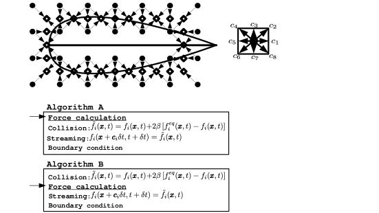
Figure 1: On top : An airfoil shaped solid object placed in a 2D cartesian grid (marked by solid circles) with a 9 velocity lattice boltzmann model. The discrete boundary points (marked by hollow squares) are placed exactly half-way between the fluid-solid links.
Below : Two possible algorithms for force calculation in a lattice boltzmann code.

In this manuscript without loss of any generality, we adhere to the simple and widely used BB treatment of the complex boundary and point out a source of ambiguity in the force computation routine. Essentially, the issue is related to the fact that LBM is a repeated sequence of collision and streaming. In absence of a boundary, the order of these operations does not matter. However, in the presence of a solid boundary, this symmetry breaks and collision and streaming operations, no longer commute with each other. Streaming is the generator of spatial translations while the boundary operator by construction must break translational invariance. Hence, in the presence of solid boundaries, the correct order of operations to calculate the flow forces, is not self evident. We describe two possible sequence of operations indicated by algorithm A and algorithm B in Fig. 1. In Fig. 2,3, we show the effect of these two approaches on two test cases, that is, flow past a 2D circular cylinder and flow past a 3D NACA0012 airfoil, at moderate Reynolds numbers. These are standard non trivial test cases extensively used for validation of numerical schemes and good amount of benchmark experimental and computational data are available for the same [20, 21, 22, 23]. To show that the discrepancy in drag values between the two algorithms, is generic, the force is computed with two discrete velocity models (D2Q9 and RD3Q41). The use of algorithm B is noticed in some literature[16, 24], however, to the best of our knowledge, a detailed comparison between the two algorithms and an analysis as to why one is better than the other, is not presented in any work.

Figure 2: Coefficient of drag vs convection time for flow past a two dimensional circular cylinder of diameter $D$ solved using a D2Q9 model at Re=100 using 80 grid points per diameter. The size of the computational domain is taken to be $(50\times 5)$D, with the cylinder symmetrically placed at $15$D from the inlet. The lattice Boltzmann results are compared with established drag values in literature [21].

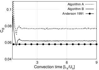
Figure 3: Coefficient of drag vs convection time for flow past a 3 dimension NACA0012 airfoil ($12\%$ thickness to chord length ratio) at AoA$=0^{\circ}$, using a RD3Q41 model at Re=5000 using 320 grid points per chord (ppc) length. The size of the computational domain is taken to be $(80\times 8\times 4)$ppc with the airfoil symmetrically placed at $24$ppc from the inlet.The lattice Boltzmann results are compared with established drag values in literature [22].

In this work, we investigate the difference in the two approaches, theoretically and numerically. In order to understand the differences, we formulate a discrete analogue of the Reynolds Transport Theorem (DRTT) in the discrete space-time setting of the lattice boltzmann equation and devise a simple and effective way for flow force calculation. The main idea in this approach is that the complex-surfaced solid can be enclosed inside a simpler cartesian-friendly bounding box, creating a control volume that facilitates balancing of momentum fluxes and accurate calculation of surface stresses on the solid boundary. The method simplifies to MEA when the outer encapsulating surface falls directly onto the discrete solid surface [25]. Hence, DRTT can be thought of as a modified MEA approach, built to tackle the errors that arise from the inability of cartesian grids to resolve complex surfaces, especially at low resolutions. To demonstrate this approach, we consider a 1D toy model as shown in Fig. 4. The standard lattice Boltzmann equation (in one dimensional space) with a relaxation term is a two step evolution

$$\begin{split}&\tilde{f}_{i}(X,t)=f_{i}(X,t)+2\beta\left[f^{eq}_{i}(X,t)-f_{i}(X,t)\right],\\ &f_{i}(X+c_{i}\delta t,t+\delta t)=\tilde{f}_{i}(X,t).\end{split}$$ (1)

A more detailed description of notations used in lattice Boltzmann literature is given in the next section. It would be convenient for further analysis to define the global momentum calculated over the control volume as,

$$J_{X}(t)=\sum_{q=1,2,3,4\cdots}\sum_{i}f_{i}(X_{q},t)c_{iX}.$$ (2)

The evolution equation for global momentum derived from Eq.(1), for a semi-infinite control volume with only $X_{1}$ as the boundary point, simplifies to :

$$\begin{split}J_{X}(t+1)-J_{X}(t)=F_{1}(X_{1},t+1)+\left(f_{-1}-f_{1}+\tilde{f_{1}}\right)_{X_{1},t},\end{split}$$ (3)

where, $F_{1}(X_{1},t+1)$ is the contribution from the boundary condition in a general case. In the simple case of a bounce-back boundary, if the boundary returns an un-collided distribution ($F_{1}(X_{1},t+1)=f_{-1}(X_{1},t)$), Eq.(3) simplifies to,

$$J_{X}(t+1)-J_{X}(t)=\left(2f_{-1}+2\beta\left[f_{1}^{eq}-f_{1}\right]\right)_{X_{1},t}.$$ (4)

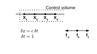
Figure 4: A D1Q3 lattice with 4 grid points$(X_{1},X_{2},X_{3},X_{4})$, where $X_{1}$ is the boundary grid point of the control volume and $X_{2}$, $X_{3}$, $X_{4}$ are the bulk grid points. In the toy example, we assume that the grid is unbounded on the right end and continues to $X_{5}$, $X_{6}$ and so on.

However global momentum balance suggests that the RHS of Eq.(4) is the total force that the boundary applies on the system. Using this example, it is easy to see that in Algorithm A, the force calculation routine (naive implementation of MEA for instance) misses out on the extra contribution, that is the second term on the RHS. If the procedure is followed for the collided populations, as per the recommendation of Algorithm B, one arrives at a simplified version of RTT,

$$J_{X}(t+1)-J_{X}(t)=2\tilde{f}_{-1}(X_{1},t),$$ (5)

where, $\tilde{f}_{i}$ represents a post-collision population.

To computationally validate our claims, we present simulations and convergence studies for NACA0012 at zero angle of attack for Reynolds numbers ranging from $10^{2}$ to $0.5\times 10^{6}$. The outline of this paper is as follows: In Sec. II, we give a brief description of LBM. In Sec. III, we review widely used methods for flow force calculation in LBM literature, namely stress integration and momentum exchange. In Sec. IV, we formulate a discrete analogue of the Reynolds tranport theorem to understand the reason behind the accuracy of Algorithm B. In Sec. V, we demonstrate some numerical simulations to validate our findings.

II Lattice Boltzmann Model

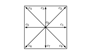
a)

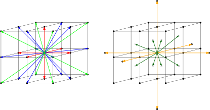
b)

Figure 5: a)Energy shells of the D2Q9 model . b) Energy shells of the RD3Q41 model: fcc-1(blue), sc-1(red), bcc-1(light green) shown on a regular lattice along with sc-2(orange), bcc-1/2(dark green).

Lattice Boltzmann method represents hydrodynamics by a discrete space-time kinetic theory. The starting point for the method, is the construction of a discrete velocity set, ${\cal C}$, consisting of $N_{d}$ discrete velocities given by ${\mathbf{c}}_{i}$ ($i=1,2,\cdots N_{d}$). The set of basic variables, ${\mathbf{f}}$, for discrete kinetic theory are populations $f_{i}({\mathbf{x}},t)$ of discrete velocities ${\mathbf{c}}_{i}$ ($i=1,2,\cdots N_{d}$), defined at location $\mathbf{x}$ and time $t$. The hydrodynamic variables are the mass density $\rho$, the fluid velocity ${\mathbf{u}}$ and scaled temperature $\theta$, defined in terms of Boltzmann constant $k_{B}$ and mass of the particle $m$, as $\theta=k_{B}T/m$. These macroscopic variables are related to the populations as,

$$\begin{split}\rho&=\sum_{i}^{N_{d}}f_{i},\\ \rho u_{\alpha}&=\sum_{i}^{N_{d}}f_{i}c_{i\alpha},\\ \rho u^{2}+D\rho\theta&=\sum_{i}^{N_{d}}f_{i}c_{i}^{2},\end{split}$$ (6)

where, $D$ signifies the dimension of the setup. For these discrete velocity models, typically the kinetic equation is written with a single relaxation (BGK) term as,

$$\frac{\partial f_{i}}{\partial t}+\boldsymbol{c}_{i}\cdot\boldsymbol{\nabla}f_{i}=-\frac{1}{\tau}\left[f_{i}-f^{eq}_{i}({\cal M}^{\rm Slow})\right],$$ (7)

where, $\tau$ is related to mean free time and $f^{eq}_{i}({\cal M}^{\rm Slow})$ is the discrete analog of Maxwell-Boltzmann distribution with ${\cal M}^{\rm Slow}$ being, the set of slow hydrodynamic moments of populations. In continuous kinetic theory, the slow moments consists of mass, momentum and energy density (${\cal M}^{\rm Slow}=\left\{\rho,\rho{\mathbf{u}},\rho u^{2}+3\rho\theta\right\}$), while in the discrete case one can often ignore energy conservation to focus on isothermal hydrodynamics only (${\cal M}^{\rm Slow}=\left\{\rho,\rho{\mathbf{u}}\right\}$). The lattice boltzmann equation is obtained by further discretizing Eq.(7) in space and time, as a sequence of discrete collisions followed by free flight(streaming) as,

$$\begin{split}&\tilde{f}_{i}(\boldsymbol{x},t)=f_{i}(\boldsymbol{x},t)+2\beta\left[f^{eq}_{i}\left(\rho(\boldsymbol{x},t),\boldsymbol{u}(\boldsymbol{x},t)\right)-f_{i}(\boldsymbol{x},t)\right],\\ &f_{i}(\boldsymbol{x}+\boldsymbol{c}_{i}\delta t,t+\delta t)=\tilde{f}_{i}(\boldsymbol{x},t).\end{split}$$ (8)

where $\beta=\delta t/(2\tau+\delta t)$. At this point, it needs to be pointed out that the same discrete evolution can also be written as free flight followed by collision as

$$\begin{split}&\hat{f}_{i}(\boldsymbol{x},t)={f}_{i}(\boldsymbol{x}-\boldsymbol{c}_{i}\delta t,t),\\ &f_{i}(\boldsymbol{x},t+\delta t)=\hat{f}_{i}(\boldsymbol{x},t)+2\beta\left[\hat{f}^{eq}_{i}\left(\rho(\boldsymbol{x},t),\boldsymbol{u}(\boldsymbol{x},t)\right)-\hat{f}_{i}(\boldsymbol{x},t)\right].\end{split}$$ (9)

It is straight-forward to see that the two versions are identical in absence of any solid boundaries. The main theoretical ingredient ensuring accurate hydrodynamics is the construction of the discrete equilibrium. Starting with a zero velocity equilibrium ($w_{i}>0$), a second order series approximation to the equilibrium is often written as,

$$f_{i}^{\rm eq}=w_{i}\,\rho\left[1+\frac{\left({\boldsymbol{u}}\cdot{\boldsymbol{c}}_{i}\right)}{\theta_{0}}+\frac{1}{2\theta_{0}^{2}}\left(\left({\boldsymbol{u}}\cdot{\boldsymbol{c}}_{i}\right)^{2}-\theta_{0}{u}^{2}\right)\right].$$ (10)

Here, it is important that the zero velocity equilibrium at a fixed temperature is positive ($w_{i}>0$) and satisfies the condition that lower order moments are same as Maxwell-Boltzmann. In particular,

$$\begin{split}\sum_{i}^{N_{d}}w_{i}&=1,\\ \sum_{i}^{N_{d}}w_{i}c_{i\alpha}c_{i\beta}&=\theta_{0}\delta_{\alpha\beta},\\ \sum_{i}^{N_{d}}w_{i}c_{i\alpha}c_{i\beta}c_{i\kappa}c_{i\gamma}&=\theta_{0}^{2}\Delta_{\alpha\beta\gamma\kappa}.\end{split}$$ (11)

These conditions on zero velocity equilibrium ensures,

$$P_{\alpha\beta}^{\rm eq}\equiv\sum_{i}f_{i}^{\rm eq}c_{i\alpha}c_{i\beta}=\rho u_{\alpha}u_{\beta}+\rho\theta_{0}\delta_{\alpha\beta}.$$ (12)

Later with higher order lattices, the method was extended for finite, but subsonic Mach number case, by ensuring that the contracted sixth order moment [26, 27] is,

$$\sum_{i}w_{i}c_{i}^{2}c_{i\alpha}c_{i\beta}c_{i\kappa}c_{i\gamma}=7\theta_{0}^{2}\Delta_{\alpha\beta\gamma\kappa}.$$ (13)

This allows one to write the equilibrium for a small departure from reference temperature, at least at zero velocity (second order in $\Delta\theta$) as,

$$\begin{split}f_{i}^{(0)}&=w_{i}\Biggl{[}1+\frac{\Delta\theta}{2}\left(c_{i}-3\right)+\frac{\Delta\theta^{2}}{8}\left(c_{i}^{2}-10c_{i}+15\right)\Biggr{]}.\end{split}$$ (14)

which gives a second order (in velocity) approximation to the equilibrium,

$$\frac{f_{i}^{\rm Eq}}{\rho\,f^{(0)}}=1+\frac{{\boldsymbol{u}}\cdot{\boldsymbol{c}}_{i}}{\theta}+\frac{\left({\boldsymbol{u}}\cdot{\boldsymbol{c}}_{i}\right)^{2}-\theta{\boldsymbol{u}}^{2}-\frac{5\bar{R}u^{2}}{6+15\bar{R}}(c_{i}^{2}-3\theta)}{2\theta^{2}},$$ (15)

The definition of $\bar{R}$ can be found in the cited reference [26]. The weights and discrete velocity set for two used models (D2Q9 and RD3Q41) are provided in Table 1 and Table 2. The energy shells for both the models is depicted in Fig. 5.

Arguably, the most crucial element of the lattice Boltzmann method is the boundary condition at a solid-fluid interface. Even though, the macroscopic boundary conditions are quite straight-forward, the mesoscopic boundary conditions on the discrete population($f_{i}(\boldsymbol{x},t)$), require some explanation. Historically, the two commonly used boundary conditions are bounce-back(BB) and diffusive boundary conditions [16, 28, 29, 6, 30]. In recent years, hybrid formulations like the diffused bounce-back boundary condition [31, 32], aimed at expanding the scope of application to a variety of problems, are also being used. In order to keep the message of this paper clear, we stick to the universally used BB boundary condition proposed by Ladd [16]. The basic implementation of BB boundary condition, assumes that a molecule hits the wall and reverses its direction.

Shells	Discrete Velocities($c_{i}$)	Weight($w_{i}$)
zero	$\left(0,0\right)$	$16/36$
SC-$1$	$\left(\pm 1,0\right),\left(0,\pm 1\right)$	$4/36$
FCC-$1$	$\left(\pm 1,\pm 1\right)$	$1/36$

Table 1: Energy shells and their corresponding velocities with weights for D2Q9 with $\theta_{0}=1/3$.

Shells	Discrete velocities($c_{i}$)	Weight($w_{i}$)
zero	$\left(0,0,0\right)$	$\left(52-323\theta_{0}+921\theta_{0}^{2}-1036\theta_{0}^{3}\right)/52$
SC-1	$\left(\pm 1,0,0\right),\left(0,\pm 1,0\right),\left(0,0,\pm 1\right)$	$\theta_{0}\left(12-38\theta_{0}+63\theta_{0}^{2}\right)/39$
SC-2	$\left(\pm 2,0,0\right),\left(0,\pm 2,0\right),\left(0,0,\pm 2\right)$	$\theta_{0}\left(3-29\theta_{0}+84\theta_{0}^{2}\right)/312$
FCC-1	$\left(\pm 1,\pm 1,0\right),\left(\pm 1,0,\pm 1\right),\left(0,\pm 1,\pm 1\right)$	$\theta_{0}\left(45\theta_{0}-6-77\theta_{0}^{2}\right)/26$
BCC-1	$\left(\pm 1,\pm 1,\pm 1\right)$	$\theta_{0}\left(20-163\theta_{0}+378\theta_{0}^{2}\right)/312$
BCC-0.5	$\left(\pm 0.5,\pm 0.5,\pm 0.5\right)$	$8\theta_{0}\left(4-17\theta_{0}+21\theta_{0}^{2}\right)/39$

Table 2: Velocities and their corresponding weights for the RD3Q41 model with $\theta_{0}=0.2948964908710633$

If $\boldsymbol{x}\in\boldsymbol{x}_{f}$ and $\boldsymbol{x}+\boldsymbol{c}_{i}\delta t\in\boldsymbol{x}_{s}$ (where $\boldsymbol{x}_{f}$ and $\boldsymbol{x}_{s}$ denote the fluid and solid domain respectively), the boundary point, $\boldsymbol{x}_{b}$, is assumed to lie at the midpoint of the vector joining $\boldsymbol{x}_{f}$ and $\boldsymbol{x}_{s}$, regardless of the physical position of the boundary (see Fig. 1). The distribution for the fluid points near the boundary is given by the boundary condition[16],

$$\begin{split}\text{Stationary wall : }&\tilde{f}_{\tilde{i}}(\boldsymbol{x}_{f},t+\delta t)=\tilde{f}_{i}(\boldsymbol{x}_{f},t)\\ \text{Moving wall : }&\tilde{f}_{\tilde{i}}(\boldsymbol{x}_{f},t+\delta t)=\tilde{f}_{i}(\boldsymbol{x}_{f},t)-2w_{i}\rho\frac{\boldsymbol{c}_{i}\cdot\boldsymbol{u}_{w}}{c_{s}^{2}}\end{split}$$ (16)

where $\tilde{i}$ is the direction opposite to $i$ and $\boldsymbol{u}_{w}$ is the velocity of the solid wall. Here, $\tilde{f}$ represents the post-collision population. There are several higher-order interpolation based curved boundary conditions in literature that address the drawbacks in accuracy of the midway bounce-back boundary condition when dealing with curved surfaces[19]. However, the essential ideas of this paper remain unchanged even with higher-order interpolation based schemes and can be transferred to the same.

III Force Computation in LBM

Very often fluid simulations require accurate determination of forces experienced by curved objects. In this section, we begin by briefly reviewing the two widely used force evaluation schemes in the •context of LBM. For fluid simulations with any method, an intuitive way of calculating forces is to perform integration of the total stress on the contact surface. This method and all its variants are referred to as stress integration (SI) algorithms. In terms of the unit normal $\boldsymbol{n}$ pointing out of the solid boundary $\partial\Omega$, the stress tensor on the boundary of a solid is

$$\boldsymbol{F}=\int_{\partial\Omega}dA\>\boldsymbol{n}\cdot(-p\boldsymbol{I}+\rho\nu[(\boldsymbol{\nabla}:\boldsymbol{u})+(\boldsymbol{\nabla}:\boldsymbol{u})^{T}])$$ (17)

where the pressure term $p=\rho\theta$ ($\theta=\theta_{0}$ for isothermal models) can be computed easily at every grid point. However, the deviatoric part ($\sigma_{\alpha\beta}$) of the stress tensor involves the velocity gradient tensor $\partial_{\alpha}u_{\beta}$, that needs to be approximated via finite differences which typically introduces additional error. This inaccuracy in calculation of velocity gradient tensor is circumvented in LBM by observation that the deviatoric stresses is evaluated as the second moment of the non-equilibrium part of the population [33]

$$\sigma_{\alpha\beta}=\left(1-\beta\right)\Sigma_{i}[f_{i}(x,t)-f_{i}^{eq}(x,t)]\left(c_{i\alpha}c_{i\beta}-\frac{\theta_{0}}{D}\delta_{\alpha\beta}\right).$$ (18)

However, LBM being a cartesian grid based method, another uncertainty in force estimation is added by the calculation of a surface normal ($\boldsymbol{n}$) for complex geometries. Thus, for a typical flow setup the SI calculation results have lower accuracy in contrast to the alternate momentum exchange method [17].

A computationally efficient and simple method is the momentum exchange (ME) algorithm [16] where, the total forces are computed as pairwise sum of momentum difference in discrete directions as populations bounces back from body surface near boundary points. In its basic version (see Fig 1), boundary is approximated quite effectively in a staircase manner at the middle of every fluid-solid links, each of which crosses the boundary and connects a fluid node. The total force experienced by the solid object is given by,

$$\boldsymbol{F}_{b}=\sum_{b}-\left[f_{\tilde{i}}(\boldsymbol{x}_{f},t)\boldsymbol{c}_{\tilde{i}}-f_{i}(\boldsymbol{x}_{f},t)\boldsymbol{c}_{i}\right],$$ (19)

where, $\tilde{i}$ is the direction opposite to $i$ and the summation runs over all fluid points next to discrete boundary. The ambiguity pointed out in the introduction of the paper, regarding the choice of algorithm (see Fig.1), plays an important role here. The momentum exchange algorithm is a limit to the more general Reynolds Transport Theorem [25]. In the next section we derive the discrete version of the Reynolds Transport Theorem and arrive at simplistic force evaluation routine for complex shaped objects.

IV Discrete Reynolds Transport Theorem

Consider a complex shaped solid object with a continuous boundary marked by $\partial\Omega$ as in Fig. 6, placed on a Cartesian grid. The solid is surrounded by fluid nodes ($\Omega$) and the discrete analogue the boundary is represented by $\partial\Omega^{D}$.

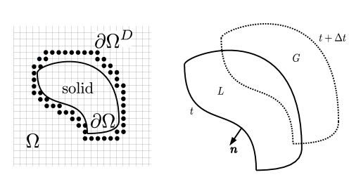
Figure 6: Left : A solid object submerged in a fluid marked by $\Omega$ on a Cartesian grid. The circular dots represent the fluid nodes that make up the discrete boundary ($\partial\Omega^{D}$) analogous to the continuous solid boundary ($\partial\Omega$).
Right : system evolving from $t$ to $t+\Delta t$.

The total momentum for all the fluid grid nodes in the bulk and boundary, is given by,

$$\begin{split}J^{\Omega}_{\alpha}(t)&=\sum_{\boldsymbol{x}\in\Omega}\sum_{i}c_{i\alpha}f_{i}(\boldsymbol{x},t),\end{split}$$ (20)

The momentum balance for the fluid points as the system evolves from $t$ to $t+\Delta t$, implies

$$J^{\Omega}_{\alpha}(t+\Delta t)=J^{\Omega}_{\alpha}(t)+J^{G}_{\alpha}(t+\Delta t)-J^{L}_{\alpha}(t)$$ (21)

where, $J^{G}_{\alpha}(t+\Delta t)$ and $J^{L}_{\alpha}(t)$ represents the gained and lost momentum at the boundary [25], as seen in Fig.6. It must be noted that $J^{G}_{\alpha}$ is calculated over the boundary grid nodes where population is added to the system and $J^{L}_{\alpha}$ is calculated over the boundary grid nodes where population leaves the system, when the system displaces from $t$ to $t+\Delta t$. The gained momentum is simply written as,

$$\begin{split}J^{G}_{\alpha}(t+\Delta t)&=\sum_{\boldsymbol{x}\in\partial\Omega^{D}}\left[\sum_{i\ni c_{i}n_{i}>0}c_{i\alpha}f_{i}(\boldsymbol{x},t+\Delta t)\right],\\ &=\sum_{\boldsymbol{x}\in\partial\Omega^{D}}\left[\sum_{i\ni c_{i}n_{i}>0}c_{i\alpha}\tilde{f}_{i}(\boldsymbol{x}-\boldsymbol{c}\Delta t,t)\right],\end{split}$$ (22)

where, $\tilde{f}_{i}$ denotes a collided population. As per the discussion in the introduction section of this article, there are two ways of calculating $J^{L}_{\alpha}(t)$, based on the choice of algorithm (A or B),

$$\begin{split}\text{Algorithm A : }&J^{L}_{\alpha}(t)=\sum_{\boldsymbol{x}\in\partial\Omega^{D}}\left[\sum_{i\ni c_{i}n_{i}\leq 0}c_{i\alpha}f_{i}(\boldsymbol{x},t)\right],\\ \text{Algorithm B : }&J^{L}_{\alpha}(t)=\sum_{\boldsymbol{x}\in\partial\Omega^{D}}\left[\sum_{i\ni c_{i}n_{i}\leq 0}c_{i\alpha}\tilde{f}_{i}(\boldsymbol{x},t)\right].\end{split}$$ (23)

The choice of Algorithm B simplifies Eq.(21) to give us the complete momentum balance for fluid nodes as,

$$\begin{split}J^{\Omega}_{\alpha}(t+\Delta t)-J^{\Omega}_{\alpha}(t)=&\sum_{\boldsymbol{x}\in\partial\Omega^{D}}\left[\sum_{i\ni c_{i}n_{i}>0}c_{i\alpha}\tilde{f}_{i}(\boldsymbol{x}-\boldsymbol{c}\Delta t,t)\right]\\ -&\sum_{\boldsymbol{x}\in\partial\Omega^{D}}\left[\sum_{i\ni c_{i}n_{i}\leq 0}c_{i\alpha}\tilde{f}_{i}(\boldsymbol{x},t)\right]\end{split}$$ (24)

The boundary surface contribution on RHS of the Eq.(24), is exactly the momentum exchange algorithm proposed by Ladd [16], whereas the choice of Algorithm A would lead to a slightly more complicated expression. Using Newton’s second law, one can estimate the forces exerted by the fluid, on submerged solid objects as,

$$\begin{split}F_{\alpha}(t)=&-\sum_{\boldsymbol{x}\in\partial\Omega^{D}}\left[\sum_{i\ni c_{i}n_{i}>0}c_{i\alpha}\tilde{f}_{i}(\boldsymbol{x}-\boldsymbol{c}\Delta t,t)\right]\\ &+\sum_{\boldsymbol{x}\in\partial\Omega^{D}}\left[\sum_{i\ni c_{i}n_{i}\leq 0}c_{i\alpha}\tilde{f}_{i}(\boldsymbol{x},t)\right].\end{split}$$ (25)

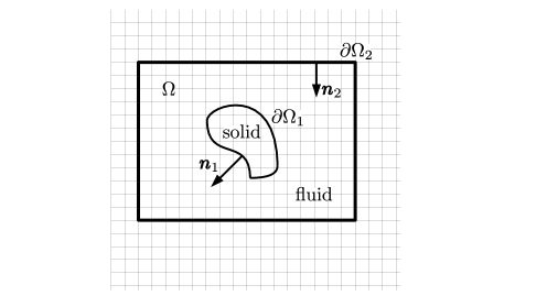
Figure 7: A complex shaped solid object placed inside a control volume. The solid surface is marked by $\partial\Omega_{1}$ and the outer rectangular control volume surface is marked by $\partial\Omega_{2}$

The first term in the force formula is dictated by the boundary condition used in the algorithm. For a simple bounce-back boundary condition, the force formula simplifies to,

$$F_{\alpha}(t)=2\sum_{\boldsymbol{x}\in\partial\Omega^{D}}\left[\sum_{i\ni c_{i}n_{i}\leq 0}c_{i\alpha}\tilde{f}_{i}(\boldsymbol{x},t)\right].$$ (26)

We extend the derivation carried out for a single boundary to a system with two boundaries as given in Fig.7, where the fluid nodes are given by $\Omega$, and are sandwiched between the two boundaries $\partial\Omega_{1}$ and $\partial\Omega_{2}$, such that the momentum balance gives,

$$\begin{split}J^{\Omega}_{\alpha}(t+\Delta t)-J^{\Omega}_{\alpha}(t)=&\sum_{\boldsymbol{x}\in\partial\Omega_{2}}\left[\sum_{i\ni c_{i}n2_{i}>0}c_{i\alpha}\tilde{f}_{i}(\boldsymbol{x}-\boldsymbol{c}\Delta t,t)\right]\\ -&\sum_{\boldsymbol{x}\in\partial\Omega_{2}}\left[\sum_{i\ni c_{i}n2_{i}\leq 0}c_{i\alpha}\tilde{f}_{i}(\boldsymbol{x},t)\right]\\ +&\sum_{\boldsymbol{x}\in\partial\Omega_{1}}\left[\sum_{i\ni c_{i}n1_{i}>0}c_{i\alpha}\tilde{f}_{i}(\boldsymbol{x}-\boldsymbol{c}\Delta t,t)\right]\\ -&\sum_{\boldsymbol{x}\in\partial\Omega_{1}}\left[\sum_{i\ni c_{i}n1_{i}\leq 0}c_{i\alpha}\tilde{f}_{i}(\boldsymbol{x},t)\right]\end{split}$$ (27)

The construction of the outer boundary $\partial\Omega_{2}$ is done in such a way that $\boldsymbol{n}_{2}$ and location of $\partial\Omega_{2}$ is trivial to resolve on a lattice. A rectangular bounding box aligned with the grid is a good example of the same. This construction helps us bypass calculations at the solid surface ($\partial\Omega_{1}$) by rearranging the Eq.(28) to,

$$\begin{split}F_{\alpha}(t)=\>\>&J^{\Omega}_{\alpha}(t)-J^{\Omega}_{\alpha}(t+\Delta t)\\ +&\sum_{\boldsymbol{x}\in\partial\Omega_{2}}\left[\sum_{i\ni c_{i}n2_{i}>0}c_{i\alpha}\tilde{f}_{i}(\boldsymbol{x}-\boldsymbol{c}\Delta t,t)\right]\\ -&\sum_{\boldsymbol{x}\in\partial\Omega_{2}}\left[\sum_{i\ni c_{i}n2_{i}\leq 0}c_{i\alpha}\tilde{f}_{i}(\boldsymbol{x},t)\right],\end{split}$$ (28)

where, $F_{\alpha}(t)$ is the force exerted by the fluid on the surface $\partial\Omega_{1}$. We label this force evaluation method as DRTT and conduct simulations in the next section to validate the method.

V Results

As a first example, we consider the flow past a circular cylinder in two dimensions, which is a regularly used benchmark case in computational fluid dynamics. The most basic calculation of the pressure coefficient on the surface of the cylinder involves calculation over boundary fluid nodes without any kind of extrapolation. The pressure coefficient at one boundary fluid node is given by,

$$C_{p}=\frac{p-p_{\infty}}{\frac{1}{2}\rho U^{2}},$$ (29)

where, $p_{\infty}$ is the far upstream pressure.

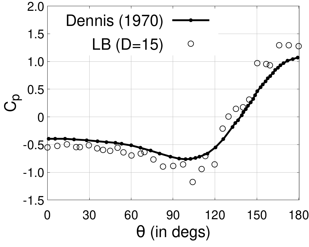
Case a)

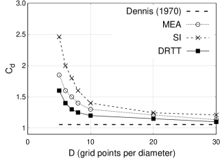
Case b)

Figure 8: The flow past a circular cylinder in 2 dimension is a good bench-marking test case for lattice boltzmann methods [20]. Fig. 8a) shows the coefficient of pressure ($C_{p}$) vs $\theta$ for Re$=100$ case. Fig. 8b) compares the drag coefficient ($C_{d}$) as a function of number of grid point per diameter for momentum exchange(ME), stress integration(SI) and discrete RTT methods (DRTT).

Fig. 8 shows the coefficient of pressure vs $\theta$ for Re$=100$ case. We see that as expected, the even at a low resolution of $D=15$, the $C_{p}$ curve is a close match with literature. Once the correctness of $C_{p}$ is established, the flow force is calculated using all the three methods discussed in the previous section. The drag coefficient over a circular cylinder of diameter D is given by,

$$C_{d}=\frac{2|F_{x}|}{\rho U^{2}D},$$ (30)

where, $x$ is taken to be the direction along the flow. The force term ($F_{x}$) is calculated using popular methods (MEA and SI), along with with the discrete Reynolds transport theorem (DRTT) algorithm. We do the convergence test for all the methods for Re$=100$ and the results are given in Fig. 8. The aspect ratio for the computational domain is taken to be $12:1$ with the length and width of the domain as $60D$ and $5D$. The cylinder of diameter $D$ is placed at $15D$ from the inlet. We can clearly see that SI does the worst among all the methods at a given resolution and henceforth we shall not discuss it in the following sections on flow past a NACA airfoil.

The simulations are run for a range of parameters, in order to study the dependence of the drag coefficient on the Reynolds number. As seen in Fig. 9, DRTT does much better than MEA at a given resolution. One can also notice that the difference between DRTT and MEA becomes more prominent at high Re where the flow starts to become unsteady.

Figure 9: The computational domain size is kept fixed with $D=15$, while the Drag coefficient ($C_{d}$) is measured for several values of Reynolds numbers. The results of MEA and DRTT are then compared with literature.

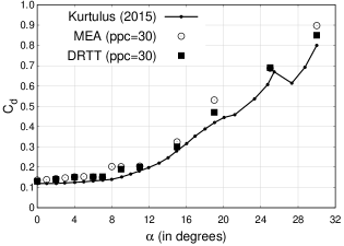
Figure 10: Flow past a NACA0012 airfoil in two dimensions, using a D2Q9 lattice model and $30$ points per chord length. The coefficient of drag ($C_{d}$) plotted against angle of attack ($\alpha$) at Re=1000.

V.1 Flow past 2D NACA0012 airfoil
(Re=1000 benchmark)

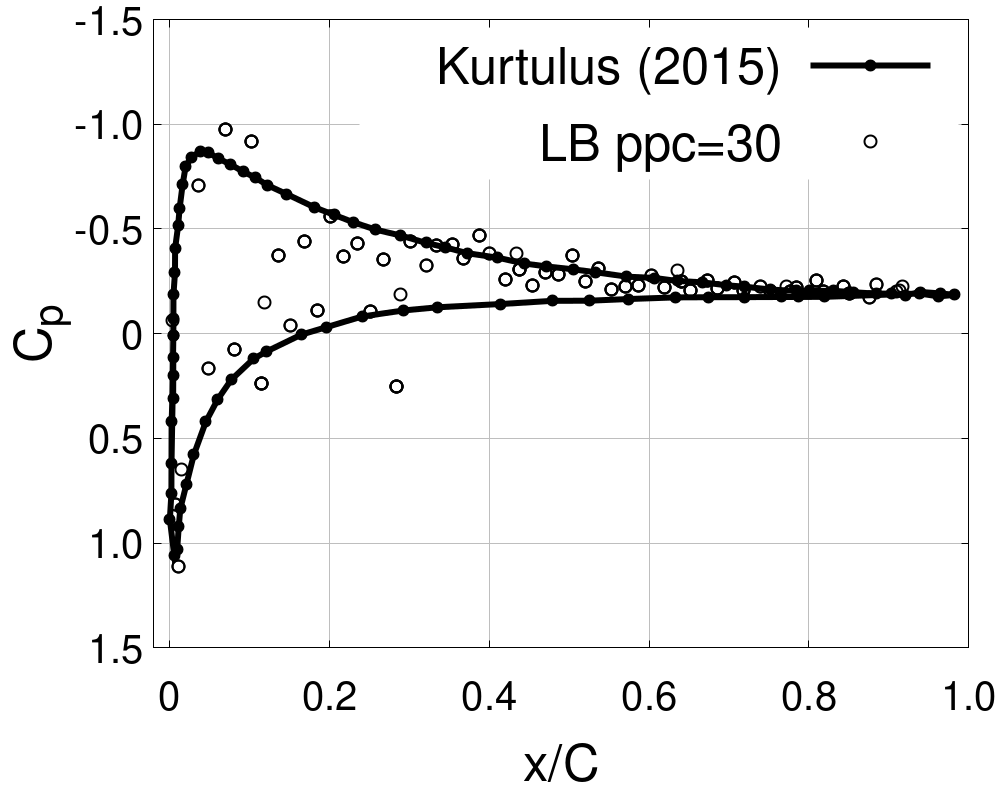
a)AoA = 7degs

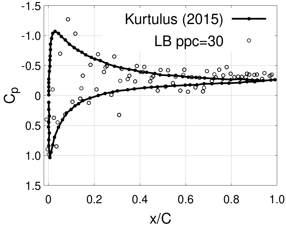
b)AoA = 9degs

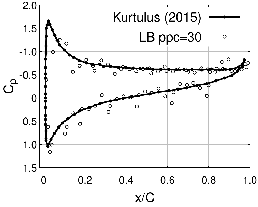
c)AoA = 15degs

Figure 11: Flow past a NACA0012 airfoil in two dimensions for Reynolds=1000 [23]. The coefficient of pressure ($C_{p}$) is calculated over the boundary fluid nodes for a computational domain size of 30 points per chord length. This is repeated for three distinct angles of attack ($\alpha=7,9,15)^{0}$ and the results are matched with literature.

The airfoil of interest in our work is the NACA0012 airfoil, that has been extensively used for validation cases for turbulence models. NACA0012 airfoil is a skewed geometry with different grid requirements in x and y directions. This makes it an important case study for algorithms like lattice Boltzmann that use uniform meshes ($\Delta x=\Delta y$). In order to validate our code, we reviewed the coefficient of pressure ($C_{p}$) measured over the airfoil surface at a Reynolds number of $1000$ and three angles of attack ($\alpha$) [23]. Fig. 11 shows us the match with literature. We plot for angle of attack$=(7,9,15)^{0}$ respectively and with a resolution of 30 points per chord.

The computational domain size is measured in the chord length ($C$) of the airfoil, such that, the number of grid points per chord length is given by $ppc$. The aspect ratio of the rectangular box is taken to be $12:1$. The length of the domain (in the direction of the flow) is taken to be $60\times C$ with the airfoil placed symmetrically at $15\times C$ from the inlet. For the next set of results, simulations are run for a Reynolds of 1000 but the angle of attack is varied starting from 0 and finishing at 30 degrees. The drag and lift coefficients are calculated using both the MEA and DRTT flow force calculation methods. Both these methods are carried out for a resolution of 30 points per chord and the results are given in Fig. 10 and Fig. 12 respectively.

The lift coefficient ($C_{l}$) is given by,

$$C_{l}=\frac{2|F_{y}|}{\rho U^{2}D}.$$ (31)

We can see that MEA and DRTT do almost equally well at low angles of attack. But as the angle of attack rises and the flow begins to separate, DRTT is able to more accurately calculate the drag and lift values. We attribute this to the fact that DRTT, being a volumetric method, does not have to resolve the complex boundary of the airfoil at low grid resolution.

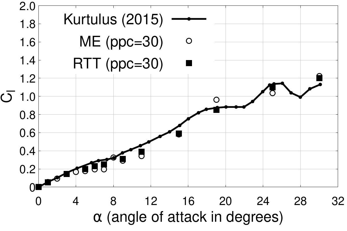
Figure 12: Flow past a NACA0012 airfoil in two dimensions for Reynolds=1000. The coefficient of lift ($C_{l}$) plotted against angle of attack ($\alpha$).

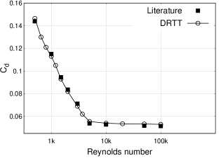
Figure 13: The coefficient of drag from a 3 dimensional simulation of NACA0012 using RD3Q41 lattice boltzmann model. Converged results have been plotted

V.2 Flow past 3D NACA0012 airfoil

The final set of simulations for this study are for a 3 dimensional case of the NACA0012 airfoil. We conducted this at a fixed angle of attack of zero degrees but increased the Reynolds from a small value of $100$ to $0.5$ million. A 41 velocity lattice boltzmann model [26] was used for the 3 dimensional simulations. The goal of the study was to validate the DRTT approach for high Re values and also compare its behaviour with MEA. The computational domain size is measured in the chord length of the airfoil ($C$). The number of grid points taken for $1C$ is given by $ppc$ (points per chord length).The aspect ratio is fixed to 10:1 in the x and y directions. The number of points in the z direction was varied with Reynolds number in order to accommodate a developing flow in the z direction at very high Reynolds. Table 3 gives details of the computational grid requirements for a converged result. The resolution demands (measured in points per chord) for a converged result vary as a function of Reynolds number. We assign an error percentage of 2 percent in order to call a result converged and tabulate the results in Table 3. The converged $C_{d}$ vs $Re$ curve as seen in Fig. 13 shows a good match with literature. Fig. 14 shows a close match with a $Re^{1/2}$ scaling which can be explained using boundary layer theory.

VI Conclusions

In this work we revisited the force evaluation methodologies in the lattice Boltzmann method. The first half of the work emphasized on the non commutativity of the streaming and collision operations when dealing with flows around solid objects. This breakdown of commutativity opens up two possibilities for force evaluation, as shown in Fig. 1, the details of which have not been fully clarified in literature. Subsequent theoretical and computational analysis showed the superiority of Algorithm B over Algorithm A. In the process of establishing the aforementioned claim, the authors have suggested a simple and elegant force evaluation routine called DRTT. The elegance of DRTT lies in its compatibility with cartesian grid based methods like lattice Boltzmann, where the accurate resolution of complex shaped geometries is a major issue. The DRTT routine is compared with the extensively used momentum-exchange method for a variety of flow problems, including flow past a two-dimensional cylinder and airfoil (NACA0012) and flow past a three-dimensional NACA0012 airfoil.

VII Acknowledgments

The authors are thankful to PK Kolluru and C Thantanapally, from SankhyaSutra Labs for their valuable inputs. SS wishes to acknowledge funding from the European Research Council under the Horizon 2020 Programme Grant Agreement n. 739964 “COPMAT”).

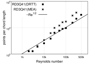
Figure 14: Total number of computational points required to correctly measure the drag values for NACA0012 using the DRTT approach. The x-axis is the Reynolds number and the y-axis is the points per chord length of NACA0012.

Re	Points per		Points in	$\%$error in $C_{d}$	$\%$error in $C_{d}$
	chord length		z-direction	(MEA)	(DRTT)
$1.0\times 10^{3}$	128		12	1.75	1.25
$1.0\times 10^{4}$	256		12	2.67	1.74
$0.1\times 10^{6}$	960		24	3.1	1.97
$0.2\times 10^{6}$	1536		48	3.22	1.87
$0.4\times 10^{6}$	2816		48	5.16	1.95
$0.5\times 10^{6}$	3072		60	9.21	2.06

Table 3: The list of grid size requirements for a 3 dimensional NACA0012 simulation using a RD3Q41 model. The aspect ratio of the computational domain is taken to be $10:1$ with the length of the channel being $10\times$points per chord.

VIII Appendix

In this section we present a basic implementation of the discrete Reynolds transport theorem for flow past a two dimensional object. The size of the control volume ($\Omega$ as seen in Fig. 7), for the simple case of 2 dimensional cylinder, is taken to be $1.5D\times 1.5D$ and the corners are marked as $cv_{x1},cv_{x2},cv_{y1},cv_{y2}$.

The basic algorithm for the force calculation using the DRTT approach is as follows:

$$\begin{split}\xrightarrow{}&\text{Mark a rectangular DRTT control volume}(\Omega)\\ \xrightarrow{}&\text{Mark boundary fluid nodes around object}(\partial\Omega_{1})\\ \xrightarrow{}&\text{Calculate total momentum in control volume}(\Omega)\\ \\ &\hskip 56.9055ptfor(i=cv_{x1},i\leq cv_{x2},i++)\\ &\hskip 56.9055ptfor(j=cv_{y1}+1,j<cv_{y2},j++)\\ &\hskip 56.9055ptJ^{\Omega}_{\alpha}(t)+=\sum_{i}c_{i\alpha}f_{i}(x,y,t)\\ \\ \xrightarrow{}&\hskip 56.9055ptfor(\text{entire fluid domain})\\ &\hskip 85.35826pt\text{Collide}\\ \\ \xrightarrow{}&\text{Inlet-Outlet boundary conditions}\\ \xrightarrow{}&\text{Force calculation on the outer rectangular surface}\\ &\text{of the control volume}(\partial\Omega_{2})\\ &\hskip 56.9055pt+\sum_{\boldsymbol{x}\in\partial\Omega_{2}}\left[\sum_{i\ni c_{i}n2_{i}>0}c_{i\alpha}\tilde{f}_{i}(\boldsymbol{x}-\boldsymbol{c}\Delta t,t)\right]\\ &\hskip 56.9055pt-\sum_{\boldsymbol{x}\in\partial\Omega_{2}}\left[\sum_{i\ni c_{i}n2_{i}\leq 0}c_{i\alpha}\tilde{f}_{i}(\boldsymbol{x},t)\right]\end{split}$$

$$\begin{split}\xrightarrow{}&\hskip 56.9055ptfor(\text{entire fluid domain})\\ &\hskip 85.35826pt\text{Advection}\\ \\ \xrightarrow{}&\text{Spectral boundary condition on the top-bottom walls}\\ &\text{and bounce-back on the object boundary}\\ \\ \xrightarrow{}&\text{Calculate total momentum in control volume}(\Omega)\\ \\ &\hskip 56.9055ptfor(i=cv_{x1},i\leq cv_{x2},i++)\\ &\hskip 56.9055ptfor(j=cv_{y1}+1,j<cv_{y2},j++)\\ &\hskip 56.9055ptJ^{\Omega}_{\alpha}(t+\Delta t)+=\sum_{i}c_{i\alpha}f_{i}(x,y,t+\Delta t)\\ \xrightarrow{}&\text{DRTT force calculation as per Eq.}\eqref{rtt7}:\\ &\hskip 56.9055ptF_{\alpha}(t)=J^{\Omega}_{\alpha}(t)-J^{\Omega}_{\alpha}(t+\Delta t)\\ &\hskip 56.9055pt+\sum_{\boldsymbol{x}\in\partial\Omega_{2}}\left[\sum_{i\ni c_{i}n2_{i}>0}c_{i\alpha}\tilde{f}_{i}(\boldsymbol{x}-\boldsymbol{c}\Delta t,t)\right]\\ &\hskip 56.9055pt-\sum_{\boldsymbol{x}\in\partial\Omega_{2}}\left[\sum_{i\ni c_{i}n2_{i}\leq 0}c_{i\alpha}\tilde{f}_{i}(\boldsymbol{x},t)\right]\end{split}$$ (32)

References

- Higuera et al. [1989] F. Higuera, S. Succi, and R. Benzi, EPL (Europhysics Letters) 9, 345 (1989).
- Higuera and Succi [1989] F. Higuera and S. Succi, EPL (Europhysics Letters) 8, 517 (1989).
- Thantanapally et al. [2013] C. Thantanapally, D. V. Patil, S. Succi, and S. Ansumali, Journal of Fluid Mechanics 728 (2013).
- Singh et al. [2011] S. Singh, G. Subramanian, and S. Ansumali, Philosophical Transactions of the Royal Society A: Mathematical, Physical and Engineering Sciences 369, 2301 (2011).
- Thampi et al. [2013] S. P. Thampi, S. Ansumali, R. Adhikari, and S. Succi, Journal of Computational Physics 234, 1 (2013).
- Ansumali et al. [2007] S. Ansumali, I. Karlin, S. Arcidiacono, A. Abbas, and N. Prasianakis, Physical review letters 98, 124502 (2007).
- Succi [2001] S. Succi, The lattice Boltzmann equation: for fluid dynamics and beyond (Oxford university press, 2001).
- Succi and Succi [2018] S. Succi and S. Succi, The lattice Boltzmann equation: for complex states of flowing matter (Oxford University Press, 2018).
- Benzi et al. [1992] R. Benzi, S. Succi, and M. Vergassola, Physics Reports 222, 145 (1992).
- Aidun and Clausen [2010] C. K. Aidun and J. R. Clausen, Annual review of fluid mechanics 42, 439 (2010).
- Chen and Doolen [1998] S. Chen and G. D. Doolen, Annual review of fluid mechanics 30, 329 (1998).
- Ansumali and Karlin [2002] S. Ansumali and I. V. Karlin, Physical Review E 66, 026311 (2002).
- Li et al. [2004] H. Li, X. Lu, H. Fang, and Y. Qian, Physical Review E 70, 026701 (2004).
- Filippova and Hänel [1998a] O. Filippova and D. Hänel, Journal of Computational physics 147, 219 (1998a).
- Inamuro et al. [2000] T. Inamuro, K. Maeba, and F. Ogino, International journal of multiphase flow 26, 1981 (2000).
- Ladd [1994a] A. J. Ladd, Journal of fluid mechanics 271, 285 (1994a).
- Mei et al. [2002] R. Mei, D. Yu, W. Shyy, and L.-S. Luo, Physical Review E 65, 041203 (2002).
- Ladd [1994b] A. J. Ladd, Journal of fluid mechanics 271, 311 (1994b).
- Mei et al. [2000] R. Mei, W. Shyy, D. Yu, and L.-S. Luo, Journal of Computational Physics 161, 680 (2000).
- Succi et al. [1989] S. Succi, E. Foti, and F. Higuera, EPL (Europhysics Letters) 10, 433 (1989).
- Dennis and Chang [1970] S. Dennis and G.-Z. Chang, Journal of Fluid Mechanics 42, 471 (1970).
- Warren et al. [1991] G. Warren, W. Anderson, J. Thomas, and S. Krist, in 10th Computational Fluid Dynamics Conference (1991) p. 1592.
- Di Ilio et al. [2018] G. Di Ilio, D. Chiappini, S. Ubertini, G. Bella, and S. Succi, Computers & Fluids 166, 200 (2018).
- Caiazzo and Junk [2008] A. Caiazzo and M. Junk, Computers & Mathematics with Applications 55, 1415 (2008).
- Giovacchini and Ortiz [2015] J. P. Giovacchini and O. E. Ortiz, Physical Review E 92, 063302 (2015).
- Kolluru et al. [2020] P. K. Kolluru, M. Atif, M. Namburi, and S. Ansumali, Physical Review E 101, 013309 (2020).
- Atif et al. [2018] M. Atif, M. Namburi, and S. Ansumali, Physical Review E 98, 053311 (2018).
- Aidun et al. [1998] C. K. Aidun, Y. Lu, and E.-J. Ding, Journal of Fluid Mechanics 373, 287 (1998).
- Noble et al. [1995] D. R. Noble, S. Chen, J. G. Georgiadis, and R. O. Buckius, Physics of Fluids 7, 203 (1995).
- Shi et al. [2011] Y. Shi, P. L. Brookes, Y. W. Yap, and J. E. Sader, Physical Review E 83, 045701 (2011).
- Krithivasan et al. [2014] S. Krithivasan, S. Wahal, and S. Ansumali, Physical Review E 89, 033313 (2014).
- Liu and Lee [2021] G. Liu and T. Lee, Computers & Fluids 220, 104884 (2021).
- Filippova and Hänel [1998b] O. Filippova and D. Hänel, Journal of computational Physics 147, 219 (1998b).