EUROPEAN ORGANIZATION FOR NUCLEAR RESEARCH (CERN)

​​​ CERN-EP-2022-198 LHCb-PAPER-2022-031 October 19, 2022

Observation of a ${J\mskip-3.0mu/\mskip-2.0mu\psi}$ $\mathchar 28931\relax$ resonance consistent with a strange pentaquark candidate in ${{{B}^{-}}}\!\rightarrow{{J\mskip-3.0mu/\mskip-2.0mu\psi}}{\mathchar 28931\relax}{\overline{p}}$ decays

LHCb Collaboration

An amplitude analysis of ${{{B}^{-}}}\!\rightarrow{{J\mskip-3.0mu/\mskip-2.0mu\psi}}{\mathchar 28931\relax}{\overline{p}}$ decays is performed using about 4400 signal candidates selected on a data sample of ${p}{p}$ collisions recorded at center-of-mass energies of 7, 8 and 13  TeV with the LHCb detector, corresponding to an integrated luminosity of 9 $\text{\,fb}^{-1}$. A narrow resonance in the ${J\mskip-3.0mu/\mskip-2.0mu\psi}$ $\mathchar 28931\relax$ system, consistent with a pentaquark candidate with strangeness, is observed with high significance. The mass and the width of this new state are measured to be $4338.2\pm 0.7\pm 0.4\text{\,Me\kern-1.00006ptV}$ and ${7.0\pm 1.2\pm 1.3\text{\,Me\kern-1.00006ptV}}$, where the first uncertainty is statistical and the second systematic. The spin is determined to be $1/2$ and negative parity is preferred. Due to the small $Q$-value of the reaction, the most precise single measurement of the ${{B}^{-}}$ mass to date, $5279.44\pm 0.05\pm 0.07\text{\,Me\kern-1.00006ptV}$, is obtained.

Submitted to Phys. Rev. Lett.

© 2024 CERN for the benefit of the LHCb collaboration. CC BY 4.0 licence.

 

The discovery of pentaquark candidates in the ${J\mskip-3.0mu/\mskip-2.0mu\psi}$ $p$ system at LHCb [1, 2] opened a new field of investigation in baryon spectroscopy. Such resonant structures with valence quark content ${P_{\psi}^{N}}^{+}$ = $c$ ​​$\overline{{c}}$$u$ $u$ $d$ have been observed only in the ${{\mathchar 28931\relax}^{0}_{b}}\rightarrow{{J\mskip-3.0mu/\mskip-2.0mu\psi}}{p}{{K}^{-}}$ decay to date. Recently, evidence for a new ${P_{\psi}^{N}}^{+}$= $c$ ​​$\overline{{c}}$$u$ $u$ $d$ candidate was found in the ${{B}^{0}_{s}}\rightarrow{{J\mskip-3.0mu/\mskip-2.0mu\psi}}{p}{\overline{p}}$ decay [4, 5], and evidence for a ${P_{\psi s}^{{\mathchar 28931\relax}}}^{0}$ = $c$ ​​$\overline{{c}}$$u$ $d$ $s$ pentaquark candidate with strangeness was found in the ${J\mskip-3.0mu/\mskip-2.0mu\psi}$ $\mathchar 28931\relax$ system in the ${{\mathchar 28932\relax}^{-}_{b}}\!\rightarrow{{J\mskip-3.0mu/\mskip-2.0mu\psi}}{\mathchar 28931\relax}{{K}^{-}}$ decay [6].

Pentaquarks are predicted within the quark model to have a minimal quark content of three quarks plus a quark-antiquark pair. Experimentally, the pentaquark candidates are found close to threshold for the production of ordinary baryon-meson states, i.e. $\varSigma_{c}^{+}\overline{D}^{0}$ and $\varSigma_{c}^{+}\overline{D}^{*0}$ for the observed ${P_{\psi}^{N}}^{+}$ states [1, 2], and ${\varXi}_{c}^{0}\overline{D}^{*0}$ for the ${P_{\psi s}^{{\mathchar 28931\relax}}}^{0}$ state [6]. Various interpretations of these states have been proposed, including tightly bound pentaquark states [7, 8, 9], loosely bound baryon-meson molecular states ([10] and references therein), and rescattering effects [11]. Hidden-charm pentaquarks with strangeness were predicted in [12, 13] as hadronic molecules, and in [14] as compact states. However, their nature is still largely unknown and further investigation is needed [15].

The ${{{B}^{-}}}\!\rightarrow{{J\mskip-3.0mu/\mskip-2.0mu\psi}}{\mathchar 28931\relax}{\overline{p}}$ decay offers the unique opportunity to simultaneously search for ${\overline{P}_{\psi}^{N}}^{-}$ and ${P_{\psi s}^{{\mathchar 28931\relax}}}^{0}$ pentaquark candidates in the ${J\mskip-3.0mu/\mskip-2.0mu\psi}$ $\overline{p}$ and ${J\mskip-3.0mu/\mskip-2.0mu\psi}$ $\mathchar 28931\relax$ systems, respectively. In particular, the phase space available in the decay allows searches for pentaquark candidates located close to different baryon-meson thresholds, such as ${\mathchar 28931\relax}^{+}_{c}$ ${D}^{0}$ for ${P_{\psi}^{N}}^{+}$, and ${\mathchar 28931\relax}^{+}_{c}$ ${D}^{-}_{s}$, ${\mathchar 28932\relax}^{+}_{c}$ ${D}^{-}$ for ${P_{\psi s}^{{\mathchar 28931\relax}}}^{0}$ candidates. Neither the ${P_{\psi s}^{{\mathchar 28931\relax}}(4459)}^{0}$ state, found in the ${{\mathchar 28932\relax}^{-}_{b}}\rightarrow{{J\mskip-3.0mu/\mskip-2.0mu\psi}}{\mathchar 28931\relax}{{K}^{-}}$ decay [6], nor the ${P_{\psi}^{N}(4337)}^{+}$ state, found in the ${{B}^{0}_{s}}\rightarrow{{J\mskip-3.0mu/\mskip-2.0mu\psi}}{p}{\overline{p}}$ decays [5], is accessible with the present analysis since they are outside of the available phase space.

The small $Q$-value of the decay, approximately $128\text{\,Me\kern-1.00006ptV}$, provides excellent mass resolution, allowing searches for narrow resonant structures. This decay was previously studied by the CMS collaboration using a sample of $450\pm 20$ signal candidates and the invariant mass distributions of the ${J\mskip-3.0mu/\mskip-2.0mu\psi}$ $\mathchar 28931\relax$, ${J\mskip-3.0mu/\mskip-2.0mu\psi}$ $\overline{p}$, $\mathchar 28931\relax$ $\overline{p}$ systems were found to be inconsistent with the pure phase-space hypothesis [16]. In this Letter, an amplitude analysis of the ${{{B}^{-}}}\!\rightarrow{{J\mskip-3.0mu/\mskip-2.0mu\psi}}{\mathchar 28931\relax}{\overline{p}}$ decay is performed using signal candidates selected on a data sample of ${p}{p}$ collisions at centre-of-mass energies of 7 TeV and 8 TeV (Run 1), and 13 TeV (Run 2), recorded between 2011 and 2018 by the LHCb detector, corresponding to an integrated luminosity of 9 $\text{\,fb}^{-1}$. In the following, the first observation of a ${P_{\psi s}^{{\mathchar 28931\relax}}}^{0}$ pentaquark candidate with strangeness in the ${{J\mskip-3.0mu/\mskip-2.0mu\psi}}{\mathchar 28931\relax}$ system is reported, which is different from the ${P_{\psi s}^{{\mathchar 28931\relax}}(4459)}^{0}$ state found in the ${{\mathchar 28932\relax}^{-}_{b}}\!\rightarrow{{J\mskip-3.0mu/\mskip-2.0mu\psi}}{\mathchar 28931\relax}{{K}^{-}}$ decay [6].

The LHCb detector is a single-arm forward spectrometer covering the pseudorapidity range $2<\eta<5$, described in detail in Refs. [17, 18, 19, 20]. The online event selection is performed by a trigger [21], comprising a hardware stage based on information from the muon system which selects ${{J\mskip-3.0mu/\mskip-2.0mu\psi}}\rightarrow{\mu^{+}}{\mu^{-}}$ decays, followed by a software stage that applies a full event reconstruction. The software trigger relies on identifying ${J\mskip-3.0mu/\mskip-2.0mu\psi}$ decays into muon pairs consistent with originating from a $B$-meson decay vertex detached from the primary $p$ $p$ collision point.

Samples of simulated events are used to study the properties of the signal mode decay ${{{{B}^{-}}}\rightarrow{{J\mskip-3.0mu/\mskip-2.0mu\psi}}{\mathchar 28931\relax}(\rightarrow{p}{{\pi}^{-}}){\overline{p}}}$ and the control mode decay ${{{{B}^{-}}}\rightarrow{{J\mskip-3.0mu/\mskip-2.0mu\psi}}{{K}^{*-}}(\rightarrow{{K}^{0}_{\mathrm{S}}}(\rightarrow{{\pi}^{+}}{{\pi}^{-}}){{\pi}^{-}})}$ . The latter are used to calibrate the distributions of simulated ${{B}^{-}}$ decays with data.

The $p$ $p$ collisions are generated using Pythia [22] with a specific LHCb configuration [23]. Decays of hadronic particles and interactions with the detector material are described by EvtGen [24], using Photos [25], and by the Geant4 toolkit [26, *Agostinelli:2002hh, 28], respectively. The signal and the control mode decays are generated from a uniform phase-space distribution.

Signal ${{B}^{-}}$ candidates are formed from combinations of ${J\mskip-3.0mu/\mskip-2.0mu\psi}$, $\mathchar 28931\relax$ and $\overline{p}$ candidates originating from a common decay vertex. The ${J\mskip-3.0mu/\mskip-2.0mu\psi}$ candidates are formed from pairs of oppositely charged tracks identified as muons and originating from a decay vertex significantly displaced from the associated $p$ $p$ primary vertex (PV). The associated PV for a given particle is the PV with the smallest impact parameter $\chi^{2}_{\rm IP}$, defined as the difference in the vertex-fit $\chi^{2}$ of a given PV reconstructed with and without the particle under consideration. The ${{\mathchar 28931\relax}\rightarrow{p}{{\pi}^{-}}}$ candidates are formed from pairs of oppositely charged tracks and selected in two different categories according to the $\mathchar 28931\relax$ decay position: i) the “long” category for early decays that allow the proton and pion candidates to be reconstructed in the vertex detector; ii) the “downstream” category for $\mathchar 28931\relax$ baryons that decay outside the vertex detector and are reconstructed in the tracking stations only. The long candidates have better mass, momentum and vertex resolution than downstream candidates. The $\overline{p}$ candidate is a charged track identified as an antiproton.

A kinematic fit [29] to the ${{B}^{-}}$ candidate is performed with the dimuon and the $p$ ${\pi}^{-}$ masses constrained to the known ${J\mskip-3.0mu/\mskip-2.0mu\psi}$ and $\mathchar 28931\relax$ masses, respectively [30]. Simulated events are weighted such that the distributions of transverse momentum, $p_{\mathrm{T}}$, and number of tracks per event for ${{B}^{-}}$ candidates match the ${{{B}^{-}}}\!\rightarrow{{J\mskip-3.0mu/\mskip-2.0mu\psi}}{{K}^{*-}}$ control-mode distributions in data. In simulation the particle identification (PID) variables for each charged track are resampled as a function of their $p$, $p_{\mathrm{T}}$ and the number of tracks in the event using ${{\mathchar 28931\relax}^{+}_{c}}\!\rightarrow{p}{{K}^{-}}{{\pi}^{+}}$ and $D^{\ast+}\rightarrow D^{0}(\rightarrow K^{-}{{\pi}^{+}})\pi^{+}$ calibration samples from data [31].

The final stage of the selection uses multivariate techniques trained with simulation and data. Separate boosted-decision-tree (BDT [32]) classifiers are employed for the four combinations of two data taking periods (Run 1 and Run 2) and two signal categories, using long and downstream reconstructed $\mathchar 28931\relax$ candidates. Each BDT is trained on simulated signal decays and data sidebands, with the $m({{J\mskip-3.0mu/\mskip-2.0mu\psi}}{\mathchar 28931\relax}{\overline{p}})$ invariant mass in the range $[5320,5360]\text{\,Me\kern-1.00006ptV}$. The variables used as input to the BDT are: the $p_{\mathrm{T}}$, the decay length significance, the angle between the momentum and the flight direction and the $\chi^{2}_{\rm IP}$ variable of the ${{B}^{-}}$ candidate; the $\chi^{2}$ probability from the kinematic fit of the candidate; the sum of the $\chi^{2}_{\rm IP}$ of the daughter particles; the angle between the momentum and the flight direction, the $\chi^{2}$ of the flight distance (only for long category candidates), the $\chi^{2}_{\rm IP}$ variables of the $\mathchar 28931\relax$ candidate; and the hadron PID for the $\overline{p}$ candidate from the ring-imaging Cherenkov detectors.

The BDT output selection criterion is chosen by maximising the figure of merit $\mathcal{S}^{2}/(\mathcal{S}+\mathcal{B})^{3/2}$, where $\mathcal{S}$ and $\mathcal{B}$ are the signal and background yield in a region of $\pm 5.3\text{\,Me\kern-1.00006ptV}$ around the known ${{B}^{-}}$ mass. To avoid a possible bias due to fluctuations of the signal yield, $\mathcal{S}$ is determined from a fit to the ${J\mskip-3.0mu/\mskip-2.0mu\psi}$ $\mathchar 28931\relax$ $\overline{p}$ invariant-mass distribution in data after applying a loose BDT selection, multiplied by the efficiency of the BDT output requirement obtained from simulation. Similarly, $\mathcal{B}$ is extracted from a fit to sideband data.

For candidates passing all selection criteria, a maximum-likelihood fit is performed to the $m({{J\mskip-3.0mu/\mskip-2.0mu\psi}}{\mathchar 28931\relax}{\overline{p}})$ distribution shown in Fig. 1, resulting in a signal yield of $4620\pm 70$. For the amplitude analysis about 4400 signal candidates are retained, with a purity of $93.0\%$ in the signal region of $\pm 2.5\sigma$ around the mass peak, where $\sigma\approx 2.1\text{\,Me\kern-1.00006ptV}$ is the mass resolution. The signal distribution is modelled by the sum of a Johnson function [33] and two Crystal Ball [34] functions sharing the same mean and width parameters determined from the fit. The tail parameters and fractions of each signal component are fixed to values obtained from a fit to simulated events. The background contribution is mainly due to random combinations of charged particles in the event and is described by a third-order Chebyshev polynomial.

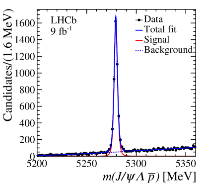
Figure 1: Invariant mass distribution of the ${J\mskip-3.0mu/\mskip-2.0mu\psi}$ $\mathchar 28931\relax$ $\overline{p}$ candidates. The data are overlaid with the results of the fit.

The Dalitz distribution of the reconstructed ${{B}^{-}}$ candidates in the signal region is shown in Fig. 2, where a horizontal band in the region around $18.8\text{\,Ge\kern-1.00006ptV}^{2}$ in the $m^{2}({{J\mskip-3.0mu/\mskip-2.0mu\psi}}{\mathchar 28931\relax})$ distribution is present. Some structure in the high $m^{2}({{J\mskip-3.0mu/\mskip-2.0mu\psi}}{\overline{p}})$ spectrum is also present. This Letter investigates the nature of these enhancements.

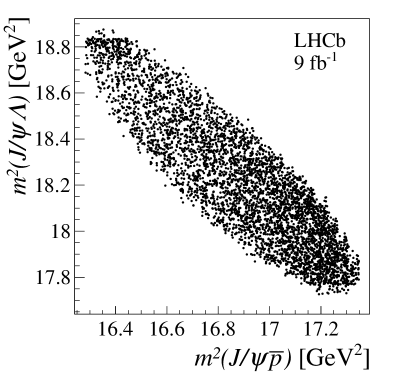
Figure 2: Dalitz distribution for ${{B}^{-}}$ candidates in the signal region.

An amplitude analysis of the ${{B}^{-}}$ candidates in the signal region is performed using a phenomenological model based on the interference of two-body resonances in the three decay chains, ${{J\mskip-3.0mu/\mskip-2.0mu\psi}}K^{*-}(\rightarrow{\mathchar 28931\relax}{\overline{p}})$, ${\mathchar 28931\relax}\overline{P}_{\psi}^{N-}(\rightarrow{{J\mskip-3.0mu/\mskip-2.0mu\psi}}{\overline{p}})$, and ${\overline{p}}{P_{\psi s}^{{\mathchar 28931\relax}}}^{0}(\rightarrow{{J\mskip-3.0mu/\mskip-2.0mu\psi}}{\mathchar 28931\relax})$, labelled as the $K^{*-}$, ${\overline{P}_{\psi}^{N}}^{-}$ and ${P_{\psi s}^{{\mathchar 28931\relax}}}^{0}$ chains, respectively. The angular information of the subsequent ${{J\mskip-3.0mu/\mskip-2.0mu\psi}}\!\rightarrow{\mu^{+}\mu^{-}}$ and ${\mathchar 28931\relax}\!\rightarrow{p}{{\pi}^{-}}$ decays are taken into account in all cases. The decay amplitudes are based on helicity formalism [35] with $C\!P$ symmetry enforced, and follow the prescriptions in Ref.[36] for the spin alignment of the different decay chains. Details about the decay amplitude definition are given in the Supplemental material [37].

The decay amplitudes are defined as a function of the six-dimensional phase space of the ${{B}^{-}}$ decay, $(m_{{\mathchar 28931\relax}{\overline{p}}},\vec{\Omega})$, described by the combined invariant mass $m_{{\mathchar 28931\relax}{\overline{p}}}$ of the $\overline{p}$ and $\mathchar 28931\relax$ pairs, and by five angular variables indicated as $\vec{\Omega}$: the cosine of the helicity angle, $\cos\theta_{{{K}^{*}}}$ $(\cos\theta_{{{J\mskip-3.0mu/\mskip-2.0mu\psi}}})$, of the $\mathchar 28931\relax$ $({\mu^{-}})$ in the $\mathchar 28931\relax$ $\overline{p}$ (${J\mskip-3.0mu/\mskip-2.0mu\psi}$) rest frame; the azimuthal angle, $\phi_{p}$ $(\phi_{\mu^{-}})$, of the ${p}$ (${\mu^{-}}$) in the rest frame of the $\mathchar 28931\relax$ (${J\mskip-3.0mu/\mskip-2.0mu\psi}$); and the cosine of the helicity angle, $\cos\theta_{{\mathchar 28931\relax}}$, of the $p$ in the rest frame of the $\mathchar 28931\relax$. The amplitude fit to determine the model parameters $\vec{\omega}$, i.e. the couplings, the masses, the widths, and lineshape parameters of different contributions, is performed by minimising the negative log-likelihood function,

$$-2\log{{\cal L}}(\vec{\omega})=-2\sum_{i}\log{\left[(1-\beta){\cal P}_{\rm{sig}}(m_{{\mathchar 28931\relax}{\overline{p}},i},\vec{\Omega_{i}}|\vec{\omega})+\beta{\cal P_{\rm{bkg}}}(m_{{\mathchar 28931\relax}{\overline{p}},i},\vec{\Omega}_{i})\right]},$$ (1)

where ${\cal P}_{\rm{sig}}$ $({\cal P}_{\rm{bkg}})$ is the probability density function (PDF) for the signal (background) component of the $i$th event, and $\beta=0.07\pm 0.01$ is the fraction of background candidates in the signal region. The signal PDF is proportional to the squared decay amplitude $|{\cal M}(m_{{\mathchar 28931\relax}{\overline{p}}},\vec{\Omega}|\vec{\omega})|^{2}$, and accounts for the phase-space element $\Phi(m_{{\mathchar 28931\relax}{\overline{p}}})$ and the reconstruction efficiency $\epsilon(m_{{\mathchar 28931\relax}{\overline{p}}},\vec{\Omega})$,

$${\cal P}_{\rm{sig}}(m_{{\mathchar 28931\relax}{\overline{p}}},\vec{\Omega}|\vec{\omega})=\frac{|{\cal M}(m_{{\mathchar 28931\relax}{\overline{p}}},\vec{\Omega}|\vec{\omega})|^{2}\Phi(m_{{\mathchar 28931\relax}{\overline{p}}})\epsilon(m_{{\mathchar 28931\relax}{\overline{p}}},\vec{\Omega})}{I(\vec{\omega})}.$$ (2)

The denominator, $I(\vec{\omega})$, normalizes the probability. The background PDF, ${\cal P}_{\rm bkg}$, is parameterized according to a six-dimensional phase-space function based on Legendre polynomials, whose coefficients are determined from the $m({{J\mskip-3.0mu/\mskip-2.0mu\psi}}{\mathchar 28931\relax}{\overline{p}})$ region ${[5200,5250]\cup[5340,5350]\text{\,Me\kern-1.00006ptV}}$. Similarly, the reconstruction efficiency is parameterized using Legendre polynomials with coefficients determined using simulated phase-space signal decays.

No well-established resonances are expected to decay into the ${{J\mskip-3.0mu/\mskip-2.0mu\psi}}{\mathchar 28931\relax}$ and ${{J\mskip-3.0mu/\mskip-2.0mu\psi}}{\overline{p}}$ final states. However, excited $K^{*-}$ resonances decaying outside of the phase space of the ${{{{B}^{-}}}\rightarrow{{J\mskip-3.0mu/\mskip-2.0mu\psi}}{\mathchar 28931\relax}{\overline{p}}}$ decay can contribute to the ${\mathchar 28931\relax}{\overline{p}}$ channel [16]. A fit including only NR contributions and $K^{*}_{4}(2045)^{-}$, $K^{*}_{2}(2250)^{-}$ and $K^{*}_{3}(2320)^{-}$ resonant amplitudes does not reproduce the data distribution. A $\chi^{2}/{\rm n.d.f.}$ of $123.2/46$ is obtained, where the $\chi^{2}$ is calculated as the largest value over the six one-dimensional fit projections and the ${\rm n.d.f.}$ is extracted from pseudoexperiments by fitting the tail of the $\chi^{2}_{\rm max}$ distribution. The simplest and most effective amplitude model used to fit the data, indicated as the nominal model in the following, comprises a narrow ${{J\mskip-3.0mu/\mskip-2.0mu\psi}}{\mathchar 28931\relax}$ structure with spin-parity $J^{P}=1/2^{-}$, whose mass and width are extracted from the amplitude fit, and two nonresonant (NR) contributions, one with $J^{P}=1^{-}$ for the ${\mathchar 28931\relax}{\overline{p}}$ system and a second one with $J^{P}=1/2^{-}$ for the ${{J\mskip-3.0mu/\mskip-2.0mu\psi}}{\overline{p}}$. The ${{J\mskip-3.0mu/\mskip-2.0mu\psi}}{\mathchar 28931\relax}$ resonance is modelled with a relativistic Breit–Wigner function as discussed in the Supplemental material [37].

The couplings are defined in the $LS$ basis, both for the ${{{B}^{-}}}\rightarrow XR$ process, and for the $R\rightarrow YZ$ process, where $X$, $Y$ and $Z$ are the final state particles, and $R=K^{*-},{\overline{P}_{\psi}^{N}}^{-}$ and ${P_{\psi s}^{{\mathchar 28931\relax}}}^{0}$ is the decay chain under consideration. Here, $L$ indicates the decay orbital angular momentum and $S$ is the sum of the spins of the decay products. In the nominal model $L=0$ is used for the production and decay of the narrow ${{J\mskip-3.0mu/\mskip-2.0mu\psi}}{\mathchar 28931\relax}$ resonance, while $L=0,1,2$ and $L=0,2$ are used in the NR(${\mathchar 28931\relax}{\overline{p}}$) system for the production and decay, respectively, and $L=0$ and $L=1$ in the NR(${{J\mskip-3.0mu/\mskip-2.0mu\psi}}{\overline{p}}$) system. Due to the small $Q$-value of the decay, higher values of the orbital momentum are suppressed. Fixing the lowest orbital momentum couplings for the NR(${{J\mskip-3.0mu/\mskip-2.0mu\psi}}{\overline{p}}$) as the normalization choice reduces the number of free parameters to sixteen: the mass, the width and the complex coupling of the ${P_{\psi s}^{{\mathchar 28931\relax}}}^{0}$ resonant contribution; four complex couplings for the NR(${\mathchar 28931\relax}{\overline{p}}$) contribution; and a complex coupling and two parameters for the second-order polynominal parameterization of the lineshape for the NR(${{J\mskip-3.0mu/\mskip-2.0mu\psi}}{\overline{p}}$) contribution.

A null-hypothesis model is used to test the significance of the ${P_{\psi s}^{{\mathchar 28931\relax}}}^{0}$ state, which comprises only two NR contributions. nominal model. The fit results for the nominal and the null-hypothesis model are shown in Fig. 3. The null-hypothesis model does not describe the data, with a corresponding $\chi^{2}_{\rm max}/{\rm n.d.f.}=120.8/47$. Using the nominal model, a good fit to data was obtained with a $\chi^{2}_{\rm max}/{\rm n.d.f.}=55.3/51$ and a $p$-value of $0.51$, computed by counting the number of pseudoexperiments above the value of $\chi^{2}_{\rm max}$ observed in data.

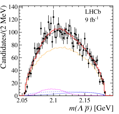
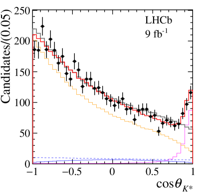
Figure 3: Distributions of invariant mass and $\cos\theta_{K^{*}}$ Fit results to data using the nominal model are superimposed. The null-hypothesis model fit results are also shown in grey. The $\varXi_{c}^{+}D^{-}$ baryon-meson threshold at 4.337  GeV is indicated with a vertical dashed line in the $m({{J\mskip-3.0mu/\mskip-2.0mu\psi}}{\mathchar 28931\relax})$ invariant mass distribution.

A new narrow ${{J\mskip-3.0mu/\mskip-2.0mu\psi}}{\mathchar 28931\relax}$ structure is observed with high significance in the nominal fit to data. Using Wilks’ theorem, a statistical significance exceeding $15\sigma$ is estimated from the value of $-2\Delta\log{\cal L}=243$ of the null-hypothesis model with respect to the nominal model. The mass and width of the new pentaquark candidate are measured to be $M_{P_{\psi s}^{{\mathchar 28931\relax}}}=4338.2\pm 0.7\text{\,Me\kern-1.00006ptV}$ and $\Gamma_{P_{\psi s}^{{\mathchar 28931\relax}}}=7.0\pm 1.2\text{\,Me\kern-1.00006ptV}$, respectively, where the uncertainties are statistical only. This represents the first observation of a strange pentaquark candidate with minimal quark content $c$ ​​$\overline{{c}}$$u$ $d$ $s$.

Alternative models are considered for systematic studies. To assess the contribution of a ${\overline{P}_{\psi}^{N}}^{-}$ pentaquark candidate, a relativistic Breit–Wigner function is used for the $m({{J\mskip-3.0mu/\mskip-2.0mu\psi}}{\overline{p}})$ lineshape instead of a 2nd order polynomial function. The value of $-2\Delta\log{\cal L}=80$ obtained with respect to the nominal fit indicates that the NR(${{J\mskip-3.0mu/\mskip-2.0mu\psi}}{\overline{p}}$) contribution is preferred over the hypothesis of a ${\overline{P}_{\psi}^{N}}^{-}$ candidate, while consistent results for the $P_{\psi s}^{{\mathchar 28931\relax}}(4338)^{0}$ state parameters are obtained. The contribution of a second narrow ${P_{\psi s}^{{\mathchar 28931\relax}}}^{0}$ resonance is added to the nominal model to parametrize the $m({{J\mskip-3.0mu/\mskip-2.0mu\psi}}{\mathchar 28931\relax})$ distribution close to the ${{\mathchar 28931\relax}^{+}_{c}}{{D}^{-}_{s}}$ threshold at $4255\text{\,Me\kern-1.00006ptV}$, and found to not be statistically significant. Using the ${\rm CL}_{s}$ method [38], an upper limit on the $P_{\psi s}^{{\mathchar 28931\relax}}(4255)^{0}$ fit fraction is set to 8.7% at a 95% confidence level. To determine the $J^{P}$ assignments, all 16 combinations of $J^{P}=1/2^{\pm},3/2^{\pm}$ are studied for the $P_{\psi s}^{{\mathchar 28931\relax}}(4338)^{0}$ and NR(${{J\mskip-3.0mu/\mskip-2.0mu\psi}}{\overline{p}}$) spin-parity hypotheses, and those with $-2\Delta\log{\cal L}>9$ with respect to the nominal fit are discarded. For the $P_{\psi s}^{{\mathchar 28931\relax}}(4338)^{0}$ state, the $J^{P}=3/2^{\pm}$ hypotheses are discarded, the $J^{P}=1/2^{-}$ assignment is preferred, while the $J^{P}=1/2^{+}$ is excluded at a 90% confidence level using the ${\rm CL}_{s}$ method [38].

Systematic uncertainties are evaluated on the mass and the width of the new pentaquark candidate, and on the fit fractions of $P_{\psi s}^{{\mathchar 28931\relax}}(4338)^{0}$, NR(${{J\mskip-3.0mu/\mskip-2.0mu\psi}}{\overline{p}}$) and NR$({{J\mskip-3.0mu/\mskip-2.0mu\psi}}{\mathchar 28931\relax})$ contributions. The uncertainties are summarised in Table 1 and are summed in quadrature for the total contribution. For each systematic uncertainty, an ensemble of 1000 pseudoexperiments, generated according to the nominal model with the same statistics as in data, is fitted with an alternative configuration that is representative of the systematic effect. The uncertainty on each parameter is determined as the mean value of the difference between the fit results of the nominal and the alternative models. The main contributions are related to the model for the decay amplitude, the bias of the fitting procedure, and the uncertanty on the reconstruction efficiency $\epsilon(m_{{\overline{p}}{\mathchar 28931\relax}},\vec{\Omega})$. For the amplitude model, the nominal value of the hadron radius for the Blatt–Weisskopf coefficients [39] is assumed to be $3\text{\,Ge\kern-1.00006ptV}^{-1}$ and varied to 1 and $5\text{\,Ge\kern-1.00006ptV}^{-1}$, taking the largest effect as a systematic uncertainty. Additional $LS$ couplings are considered with respect to the nominal model, in particular the $L,S=1,1$ ($L,S=2,3/2$) coupling for the production (decay) of $P_{\psi s}^{{\mathchar 28931\relax}}(4338)^{0}$ contribution, and the $L,S=1,1$ coupling for the NR$({{J\mskip-3.0mu/\mskip-2.0mu\psi}}{\overline{p}})$ contribution. A relativistic Breit–Wigner function is used instead of the 2nd order polynominal for the lineshape of the NR$({{J\mskip-3.0mu/\mskip-2.0mu\psi}}{\overline{p}})$ contribution. Moreover, a model with $J^{P}=1/2^{+}$ assignment to the $P_{\psi s}^{{\mathchar 28931\relax}}(4338)^{0}$ state is also considered. Finally, the behaviour of the maximum-likelihood estimator is studied using 1000 pseudoesperiments. Biases on the fit parameters are present due to the limited sample size and are assigned as systematic uncertainties. For the reconstruction efficiency, the nominal efficiency function based on decays from either the long or downstream $\mathchar 28931\relax$ category and the largest effect is considered as systematic uncertainty.

Additional systematic uncertainties account for the limited knowledge of the ${\mathchar 28931\relax}\rightarrow{p}{{\pi}^{-}}$ decay amplitude parameters [40, 30], the background parameterization, and the effect of the resolution on the $m({{J\mskip-3.0mu/\mskip-2.0mu\psi}}{\mathchar 28931\relax})$ invariant mass. The nominal background parameterization ${\cal P}_{\rm{bkg}}$ is obtained from the distributions of candidates in the $m({{J\mskip-3.0mu/\mskip-2.0mu\psi}}{\mathchar 28931\relax}{\overline{p}})$ range ${[5200,5250]\cup[5340,5350]\text{\,Me\kern-1.00006ptV}}$, while the parameterization obtained from the region $[5295,5315]\text{\,Me\kern-1.00006ptV}$ is used to assess systematic effects. The background fraction $\beta=0.07\pm 0.01$ is also varied within uncertainties. The effect of the invariant mass resolution, about $1\text{\,Me\kern-1.00006ptV}$ on average on $m({{J\mskip-3.0mu/\mskip-2.0mu\psi}}{\mathchar 28931\relax})$, is estimated by smearing the invariant mass distributions of 1000 pseudoexperiments and fitting them using the nominal model.

Table 1: Systematic uncertainties on the mass ($M_{P_{\psi s}^{{\mathchar 28931\relax}}}$) and width ($\Gamma_{P_{\psi s}^{{\mathchar 28931\relax}}}$) of the ${P_{\psi s}^{{\mathchar 28931\relax}}}^{0}$ state (in  MeV), and on the fit fractions $f_{P_{\psi s}^{{\mathchar 28931\relax}}}$, $f_{\textrm{NR}({{J\mskip-3.0mu/\mskip-2.0mu\psi}}{\overline{p}})}$ and $f_{\textrm{NR}({\mathchar 28931\relax}{\overline{p}})}$ of the pentaquark candidate and nonresonant contributions (in %).

Source	$M_{P_{\psi s}^{{\mathchar 28931\relax}}}$	$\Gamma_{P_{\psi s}^{{\mathchar 28931\relax}}}$	$f_{P_{\psi s}^{{\mathchar 28931\relax}}}$	$f_{\textrm{NR}({{J\mskip-3.0mu/\mskip-2.0mu\psi}}{\overline{p}})}$	$f_{\textrm{NR}({\mathchar 28931\relax}{\overline{p}})}$
Hadron radius	$0.1$	$0.4$	$0.3$	$0.2$	$0.2$
$LS$ values	$0.3$	$0.1$	$0.8$	$0.7$	$0.6$
Breit–Wigner ${\overline{P}_{\psi}^{N}}^{-}$	$0.1$	$0.9$	$0.8$	…	…
$J^{P}({P_{\psi s}^{{\mathchar 28931\relax}}}^{0})$ assignment	$0.1$	$0.9$	$1.2$	$0.4$	$0.9$
Fitting procedure	$0.1$	$0.2$	$0.1$	$1.0$	$1.1$
Efficiency	$0.02$	$0.19$	$0.02$	$0.3$	$0.2$
${\mathchar 28931\relax}$ decay parameters	$0.02$	$0.04$	$0.01$	$0.3$	$0.2$
Background	$0.01$	$0.05$	$0.96$	$0.4$	$0.7$
Mass resolution	$0.01$	$0.03$	$0.01$	$0.1$	$0.1$
Total	$0.4$	$1.3$	$1.9$	$1.4$	$1.7$

The mass and width of the new pentaquark candidate are measured to be ${M_{P_{\psi s}^{{\mathchar 28931\relax}}}=4338.2\pm 0.7\pm 0.4\text{\,Me\kern-1.00006ptV}}$ and $\Gamma_{P_{\psi s}^{{\mathchar 28931\relax}}}=7.0\pm 1.2\pm 1.3\text{\,Me\kern-1.00006ptV}$; the measured fit fractions are $f_{P_{\psi s}^{{\mathchar 28931\relax}}}=0.125\pm 0.007\pm 0.019$, $f_{{\rm NR}({{J\mskip-3.0mu/\mskip-2.0mu\psi}}{\overline{p}})}=0.840\pm 0.022\pm 0.014$, and $f_{{\rm NR}({\mathchar 28931\relax}{\overline{p}})}=0.113\pm 0.013\pm 0.017$, for the resonant ${P_{\psi s}^{{\mathchar 28931\relax}}}^{0}$ state, the nonresonant ${\textrm{NR}({p}{{J\mskip-3.0mu/\mskip-2.0mu\psi}})}$, and ${\textrm{NR}({p}{\kern 1.79993pt\overline{\kern-1.79993pt\mathchar 28931\relax}})}$ contributions, respectively. The first uncertainty is statistical and the second systematic. The $J^{P}=1/2^{-}$ quantum numbers for the ${P_{\psi s}^{{\mathchar 28931\relax}}(4338)^{0}}$ state are preferred; $J=1/2$ is established and positive parity can be excluded at 90% confidence level. Due to the small $Q$-value of the decay, the most precise single measurement to date of the ${{B}^{-}}$ mass, $5279.44\pm 0.05\pm 0.07\text{\,Me\kern-1.00006ptV}$, is performed. This measurement is based on signal candidates with $\mathchar 28931\relax$ baryons in the long category. Systematic uncertainties on the ${{B}^{-}}$ mass include uncertainties on particle interactions with the detector material ($0.030\text{\,Me\kern-1.00006ptV}$), momentum scaling due to imperfections in the magnetic-field mapping ($0.039\text{\,Me\kern-1.00006ptV}$), and the choice of the signal and background fit model ($0.050\text{\,Me\kern-1.00006ptV}$). Systematic uncertainties from knowledge of the ${{J\mskip-3.0mu/\mskip-2.0mu\psi}},{\mathchar 28931\relax}$ and ${p}$ masses are negligible.

In conclusion, an amplitude analysis of the ${{{B}^{-}}}\rightarrow{{J\mskip-3.0mu/\mskip-2.0mu\psi}}{\mathchar 28931\relax}{\overline{p}}$ decay is performed using about 4400 signal candidates, selected on data collected by the LHCb experiment between 2011 and 2018 and corresponding to an integrated luminosity of $9\text{\,fb}^{-1}$. A new resonant structure in the ${{J\mskip-3.0mu/\mskip-2.0mu\psi}}{\mathchar 28931\relax}$ system is found with high statistical significance, representing the first observation of a pentaquark candidate with strange quark content, named the ${P_{\psi s}^{{\mathchar 28931\relax}}(4338)^{0}}$ state, with spin $J=1/2$ assigned and parity $P=-1$ preferred. No evidence for additional resonant states, either $P_{\psi s}^{{\mathchar 28931\relax}}(4255)^{0}$ or ${\overline{P}_{\psi}^{N}}^{-}$ pentaquark candidates or excited $K^{*-}$ resonances, is found from the fit to data. The new ${P_{\psi s}^{{\mathchar 28931\relax}}(4338)^{0}}$ state is found at the threshold for ${{\mathchar 28932\relax}^{+}_{c}}{{D}^{-}}$ baryon-meson production, which is relevant for the interpretation of its nature.

Supplemental Material

Appendix A Amplitude model

The amplitude model is constructed using helicity formalism [35] following the prescription for final particle spin matching described in Ref. [36]. The amplitude $O^{X}_{\lambda_{1},\lambda_{2},\lambda_{3}}$ describes the decay amplitude for the ${{B}^{-}}$ to the ${J\mskip-3.0mu/\mskip-2.0mu\psi}$ $\mathchar 28931\relax$ $\overline{p}$ final state via the $K^{*-},{\overline{P}_{\psi}^{N}}^{-},{P_{\psi s}^{{\mathchar 28931\relax}}}^{0}$ decay chains as follows,

$$O^{K^{*}}_{\lambda_{{J\mskip-3.0mu/\mskip-2.0mu\psi}},\lambda_{{\mathchar 28931\relax}},\lambda_{\overline{p}}}(m^{2}_{{{J\mskip-3.0mu/\mskip-2.0mu\psi}}{{\mathchar 28931\relax}}},m^{2}_{{{\mathchar 28931\relax}}{\overline{p}}}) =\sum_{j^{K^{*}}}\sum_{\{\lambda^{\prime}\}}\sqrt{\frac{2j^{K^{*}}+1}{4\pi}}\,H^{B^{-}\rightarrow K^{*}{{J\mskip-3.0mu/\mskip-2.0mu\psi}}}_{\lambda_{{J\mskip-3.0mu/\mskip-2.0mu\psi}}^{\prime}}\,R(m^{2}_{{{\mathchar 28931\relax}}{\overline{p}}})\,d^{j^{K^{*}}}_{\lambda_{{J\mskip-3.0mu/\mskip-2.0mu\psi}}^{\prime},\lambda_{{\mathchar 28931\relax}}^{\prime}-\lambda_{\overline{p}}^{\prime}}(\theta_{K^{*}})$$

$$\times H^{K^{*}\rightarrow{{\mathchar 28931\relax}}{\overline{p}}}_{\lambda_{{\mathchar 28931\relax}}^{\prime},\lambda_{\overline{p}}^{\prime}}\delta_{\lambda_{{J\mskip-3.0mu/\mskip-2.0mu\psi}}^{\prime},\lambda_{{J\mskip-3.0mu/\mskip-2.0mu\psi}}}\,d^{1/2}_{\lambda_{{\mathchar 28931\relax}}^{\prime},\lambda_{{\mathchar 28931\relax}}}(\zeta^{{{\mathchar 28931\relax}}}_{B{\overline{p}}})\,d^{1/2}_{\lambda_{\overline{p}}^{\prime},\lambda_{\overline{p}}}(-\zeta^{{\overline{p}}}_{B{{\mathchar 28931\relax}}})\times(-1)^{j^{{{J\mskip-3.0mu/\mskip-2.0mu\psi}}}-\lambda_{{J\mskip-3.0mu/\mskip-2.0mu\psi}}^{\prime}}(-1)^{j^{\overline{p}}-\lambda_{\overline{p}}^{\prime}},$$

$$O^{P_{\psi}^{N}}_{\lambda_{{J\mskip-3.0mu/\mskip-2.0mu\psi}},\lambda_{{\mathchar 28931\relax}},\lambda_{\overline{p}}}(m^{2}_{{{J\mskip-3.0mu/\mskip-2.0mu\psi}}{{\mathchar 28931\relax}}},m^{2}_{{{\mathchar 28931\relax}}{\overline{p}}}) =\sum_{j^{P_{\psi}^{N}}}\sum_{\{\lambda^{\prime}\}}\sqrt{\frac{2j^{P_{\psi}^{N}}+1}{4\pi}}\,H^{B^{-}\rightarrow P_{\psi}^{N}{{\mathchar 28931\relax}}}_{\lambda_{{\mathchar 28931\relax}}^{\prime}}\,R(m^{2}_{{\overline{p}}{{J\mskip-3.0mu/\mskip-2.0mu\psi}}})\,d^{j^{P_{\psi}^{N}}}_{\lambda_{{\mathchar 28931\relax}}^{\prime},\lambda_{\overline{p}}^{\prime}-\lambda_{{J\mskip-3.0mu/\mskip-2.0mu\psi}}^{\prime}}(\theta_{P_{\psi}^{N}})$$

$$\times H^{P_{\psi}^{N}\rightarrow{\overline{p}}{{J\mskip-3.0mu/\mskip-2.0mu\psi}}}_{\lambda_{\overline{p}}^{\prime},\lambda_{{J\mskip-3.0mu/\mskip-2.0mu\psi}}^{\prime}}d^{1}_{\lambda_{{J\mskip-3.0mu/\mskip-2.0mu\psi}}^{\prime},\lambda_{{J\mskip-3.0mu/\mskip-2.0mu\psi}}}(-\zeta^{{{J\mskip-3.0mu/\mskip-2.0mu\psi}}}_{B{\overline{p}}})\,\delta_{\lambda_{{\mathchar 28931\relax}}^{\prime},\lambda_{{\mathchar 28931\relax}}}\,d^{1/2}_{\lambda_{\overline{p}}^{\prime},\lambda_{\overline{p}}}(\zeta^{{\overline{p}}}_{B{{J\mskip-3.0mu/\mskip-2.0mu\psi}}})\times(-1)^{j^{{\mathchar 28931\relax}}-\lambda_{\mathchar 28931\relax}^{\prime}}(-1)^{j^{{J\mskip-3.0mu/\mskip-2.0mu\psi}}-\lambda_{{J\mskip-3.0mu/\mskip-2.0mu\psi}}^{\prime}},$$

$$O^{{{P}_{\psi s}^{{\mathchar 28931\relax}}}}_{\lambda_{{J\mskip-3.0mu/\mskip-2.0mu\psi}},\lambda_{{\mathchar 28931\relax}},\lambda_{\overline{p}}}(m^{2}_{{{J\mskip-3.0mu/\mskip-2.0mu\psi}}{{\mathchar 28931\relax}}},m^{2}_{{{\mathchar 28931\relax}}{\overline{p}}}) =\sum_{j^{{P}_{\psi s}^{{\mathchar 28931\relax}}}}\sum_{\{\lambda^{\prime}\}}\sqrt{\frac{2j^{{P}_{\psi s}^{{\mathchar 28931\relax}}}+1}{4\pi}}\,H^{B^{-}\rightarrow{P}_{\psi s}^{{\mathchar 28931\relax}}{\overline{p}}}_{\lambda_{\overline{p}}^{\prime}}\,R(m^{2}_{{{J\mskip-3.0mu/\mskip-2.0mu\psi}}{{\mathchar 28931\relax}}})\,d^{J^{{P}_{\psi s}^{{\mathchar 28931\relax}}}}_{\lambda_{\overline{p}},\lambda_{{J\mskip-3.0mu/\mskip-2.0mu\psi}}^{\prime}-\lambda_{{\mathchar 28931\relax}}^{\prime}}(\theta_{{P}_{\psi s}^{{\mathchar 28931\relax}}})$$

$$\times H^{{P}_{\psi s}^{{\mathchar 28931\relax}}\rightarrow{{J\mskip-3.0mu/\mskip-2.0mu\psi}}{{\mathchar 28931\relax}}}_{\lambda_{{J\mskip-3.0mu/\mskip-2.0mu\psi}}^{\prime},\lambda_{{\mathchar 28931\relax}}^{\prime}}d^{1}_{\lambda_{{J\mskip-3.0mu/\mskip-2.0mu\psi}}^{\prime},\lambda_{{J\mskip-3.0mu/\mskip-2.0mu\psi}}}(\zeta^{{{J\mskip-3.0mu/\mskip-2.0mu\psi}}}_{B{{\mathchar 28931\relax}}})\,d^{1/2}_{\lambda_{{\mathchar 28931\relax}}^{\prime},\lambda_{{\mathchar 28931\relax}}}(-\zeta^{{{\mathchar 28931\relax}}}_{B{{J\mskip-3.0mu/\mskip-2.0mu\psi}}})\,\delta_{\lambda_{\overline{p}}^{\prime},\lambda_{\overline{p}}}\times(-1)^{j^{{\overline{p}}}-\lambda_{\overline{p}}^{\prime}}(-1)^{j^{{\mathchar 28931\relax}}-\lambda_{\mathchar 28931\relax}^{\prime}},$$

where $j^{X}$ is the total angular momentum of the different contributions in the ${X=K^{*-},\overline{P}_{\psi}^{N-}}$ and ${P_{\psi s}^{{\mathchar 28931\relax}}}^{0}$ decay chains, respectively, and $\{\lambda^{\prime}\}$ are the helicities of the final particles before spin rotations. The angle, $\zeta^{i}_{Bk}$, is between the $B^{-}$ and the particle $k$ in rest frame $i$. The coupling, $H_{\lambda^{\prime}}^{A\rightarrow BC}$, is the helicity coupling of a two-body decay $A\rightarrow BC$, $R$ is the line shape and $d^{j}_{\lambda_{A},\lambda_{B}-\lambda_{C}}$ is the small Wigner function. The angle, $\theta_{X}$, is the helicity angle of particle $X$, which is calculated using the $\mathchar 28931\relax$ in the $K^{*-}$ rest frame, and either the $\overline{p}$ in the $\overline{P}_{\psi}^{N-}$ rest frame, or the ${J\mskip-3.0mu/\mskip-2.0mu\psi}$ in the $P_{\psi s}^{{\mathchar 28931\relax}}$ rest frame.

The total decay amplitude is obtained by including the ${{J\mskip-3.0mu/\mskip-2.0mu\psi}}\rightarrow{\mu^{+}}\mu^{-}$ and the ${\mathchar 28931\relax}\rightarrow{p}{{\pi}^{-}}$ decay amplitudes

$$A_{\lambda_{\overline{p}},\lambda_{p},\Delta\mu}(m_{{\overline{p}}{\mathchar 28931\relax}},\vec{\Omega}) =\sum_{\lambda_{\bar{\Lambda}},\lambda_{{J\mskip-3.0mu/\mskip-2.0mu\psi}}}\left(O^{K^{*-}}+O^{P_{\psi}^{N-}}+O^{{P_{\psi s}^{{\mathchar 28931\relax}}}^{0}}\right)_{\lambda_{{J\mskip-3.0mu/\mskip-2.0mu\psi}},\lambda_{{\mathchar 28931\relax}},\lambda_{\overline{p}}}(m^{2}_{{{J\mskip-3.0mu/\mskip-2.0mu\psi}}{{\mathchar 28931\relax}}},m^{2}_{{{\mathchar 28931\relax}}{\overline{p}}})$$

$$\hskip 56.9055pt\times D^{1*}_{\lambda_{{J\mskip-3.0mu/\mskip-2.0mu\psi}},\Delta_{\mu}}(\phi_{\mu^{-}},\theta_{{J\mskip-3.0mu/\mskip-2.0mu\psi}},0)\,H^{{{\mathchar 28931\relax}}\rightarrow{p}\pi}_{\lambda_{p}}D^{1/2*}_{\lambda_{{\mathchar 28931\relax}},\lambda_{p}}(\phi_{p},\theta_{{\mathchar 28931\relax}},0),$$ (4)

where $D^{j*}_{\lambda_{A},\lambda_{B}-\lambda_{C}}(\phi,\theta,0)$ is the Wigner $D$ matrix, equal to $e^{i\lambda_{A}\phi}d^{j}_{\lambda_{A},\lambda_{B}-\lambda_{C}}(\theta)$, $\phi_{\mu^{-}},\theta_{{J\mskip-3.0mu/\mskip-2.0mu\psi}},\phi_{p},\theta_{{\mathchar 28931\relax}}$ are the azimuthal and polar angles of $\mu^{-}$ and $p$ in the ${{J\mskip-3.0mu/\mskip-2.0mu\psi}}$ and ${\mathchar 28931\relax}$ rest frames, respectively. The axes in the $B$ rest frame are defined as follows,

$$\begin{aligned} \hat{x}_{{J\mskip-3.0mu/\mskip-2.0mu\psi}}&=\hat{y}_{{J\mskip-3.0mu/\mskip-2.0mu\psi}}\times\hat{z}_{{J\mskip-3.0mu/\mskip-2.0mu\psi}},\\ \hat{y}_{{J\mskip-3.0mu/\mskip-2.0mu\psi}}&=\frac{\vec{p}_{\overline{p}}^{B}\times\vec{p}_{{J\mskip-3.0mu/\mskip-2.0mu\psi}}^{B}}{|\vec{p}_{{J\mskip-3.0mu/\mskip-2.0mu\psi}}^{B}\times\vec{p}_{\overline{p}}^{B}|},\\ \hat{z}_{{J\mskip-3.0mu/\mskip-2.0mu\psi}}&=\frac{\vec{p}_{{J\mskip-3.0mu/\mskip-2.0mu\psi}}^{B}}{|\vec{p}_{{J\mskip-3.0mu/\mskip-2.0mu\psi}}^{B}|},\\ \end{aligned} \begin{aligned} \hat{x}_{{\mathchar 28931\relax}}&=\hat{y}_{{\mathchar 28931\relax}}\times\hat{z}_{{\mathchar 28931\relax}},\\ \hat{y}_{{\mathchar 28931\relax}}&=\frac{\vec{p}_{\overline{p}}^{B}\times\vec{p}_{{\mathchar 28931\relax}}^{B}}{|\vec{p}_{{\mathchar 28931\relax}}^{B}\times\vec{p}_{\overline{p}}^{B}|},\\ \hat{z}_{{\mathchar 28931\relax}}&=\frac{\vec{p}_{{\mathchar 28931\relax}}^{B}}{|\vec{p}_{{\mathchar 28931\relax}}^{B}|},\end{aligned}$$ (5)

where the symbol $\hat{x}$ refers to $\vec{x}/|x|$. In Eq. 4, $\Delta\mu$ is the difference of the muon helicities. For the ${{J\mskip-3.0mu/\mskip-2.0mu\psi}}\rightarrow{\mu^{+}}\mu^{-}$ decay, the coupling can be absorbed into the other couplings of the total decay amplitude and therefore is not fit. Indeed, there is only one coupling because the process with $\Delta\mu=0$ is highly suppressed. So, $\Delta\mu$ can only take values $1$ and $-1$, and both choices lead to the same helicity coupling due to parity conservation.

Enforcing $C\!P$ conservation, the helicity couplings for $B^{-}$ and ${{B}^{+}}$ decays are the same. The matrix-element formula is the same for charge-conjugate decays, but all azimuthal angles must change sign due to charge-parity transformation, i.e. $\phi_{p}\rightarrow-\phi_{{\overline{p}}}$ and $\phi_{\mu^{-}}\rightarrow-\phi_{\mu^{+}}$.

The ${\kern 1.79993pt\overline{\kern-1.79993pt\mathchar 28931\relax}}\rightarrow{\overline{p}}{{\pi}^{+}}$ decay parameters are defined by

$$\alpha_{+}=\frac{|H^{{\kern 1.25995pt\overline{\kern-1.25995pt\mathchar 28931\relax}}\rightarrow{\overline{p}}{{\pi}^{+}}}_{1/2}|^{2}-|H^{{\kern 1.25995pt\overline{\kern-1.25995pt\mathchar 28931\relax}}\rightarrow{\overline{p}}{{\pi}^{+}}}_{-1/2}|^{2}}{|H^{{\kern 1.25995pt\overline{\kern-1.25995pt\mathchar 28931\relax}}\rightarrow{\overline{p}}{{\pi}^{+}}}_{1/2}|^{2}+|H^{{\kern 1.25995pt\overline{\kern-1.25995pt\mathchar 28931\relax}}\rightarrow{\overline{p}}{{\pi}^{+}}}_{-1/2}|^{2}},$$

$$\beta_{+}=\frac{2\textrm{Im}(H^{{\kern 1.25995pt\overline{\kern-1.25995pt\mathchar 28931\relax}}\rightarrow{\overline{p}}{{\pi}^{+}}}_{1/2}H^{{\kern 1.25995pt\overline{\kern-1.25995pt\mathchar 28931\relax}}\rightarrow{\overline{p}}{{\pi}^{+}}*}_{-1/2})}{|H^{{\kern 1.25995pt\overline{\kern-1.25995pt\mathchar 28931\relax}}\rightarrow{\overline{p}}{{\pi}^{+}}}_{1/2}|^{2}+|H^{{\kern 1.25995pt\overline{\kern-1.25995pt\mathchar 28931\relax}}\rightarrow{\overline{p}}{{\pi}^{+}}}_{-1/2}|^{2}},$$ (6)

$$\gamma_{+}=\frac{2\textrm{Re}(H^{{\kern 1.25995pt\overline{\kern-1.25995pt\mathchar 28931\relax}}\rightarrow{\overline{p}}{{\pi}^{+}}}_{1/2}H^{{\kern 1.25995pt\overline{\kern-1.25995pt\mathchar 28931\relax}}\rightarrow{\overline{p}}{{\pi}^{+}}*}_{-1/2})}{|H^{{\kern 1.25995pt\overline{\kern-1.25995pt\mathchar 28931\relax}}\rightarrow{\overline{p}}{{\pi}^{+}}}_{1/2}|^{2}+|H^{{\kern 1.25995pt\overline{\kern-1.25995pt\mathchar 28931\relax}}\rightarrow{\overline{p}}{{\pi}^{+}}}_{-1/2}|^{2}},$$

which satisfy the relation,

$$\alpha^{2}_{+}+\beta^{2}_{+}+\gamma^{2}_{+}=1.$$

It is convenient to express $\beta_{+}$ and $\gamma_{+}$ in terms of an angle $\phi_{+}$ defined as

$$\beta_{+}=\sqrt{1-\alpha^{2}_{+}}\sin{\phi_{+}},$$ (7)

$$\gamma_{+}=\sqrt{1-\alpha^{2}_{+}}\cos{\phi_{+}}.$$

Enforcing $C\!P$ conservation, the following relations hold,

$$H^{{\kern 1.25995pt\overline{\kern-1.25995pt\mathchar 28931\relax}}\rightarrow{\overline{p}}{{\pi}^{+}}}_{\mp 1/2}=\eta_{{\mathchar 28931\relax}}\eta_{{p}}\eta_{\pi}(-1)^{J_{{\mathchar 28931\relax}}-J_{{p}}-J_{\pi}}H^{{\mathchar 28931\relax}\rightarrow{p}{{\pi}^{-}}}_{\pm 1/2}=-H^{{\mathchar 28931\relax}\rightarrow{p}{{\pi}^{-}}}_{\pm 1/2}.$$ (8)

This leads to

$$\alpha_{+}=-\alpha_{-},$$

$$\beta_{+}=-\beta_{-},$$

$$\gamma_{+}=\gamma_{-},$$

$$\tan{\phi_{+}}=-\tan{\phi_{-}},$$ (9)

where $\alpha_{-}$, $\beta_{-}$ and $\gamma_{-}$ are obtained following Eq. A but using the couplings of the conjugate decay.

If the complex helicity coupling $H^{{\kern 1.25995pt\overline{\kern-1.25995pt\mathchar 28931\relax}}\!\rightarrow{\overline{p}}{{\pi}^{+}}}_{1/2}$ is set to (1,0), then $H^{{\kern 1.25995pt\overline{\kern-1.25995pt\mathchar 28931\relax}}\!\rightarrow{\overline{p}}{{\pi}^{+}}}_{-1/2}=\sqrt{\frac{1-\alpha_{+}}{1+\alpha_{+}}}e^{-i\phi_{+}}$. The values of $\alpha_{+}$ and $\phi_{+}$ are fixed to $-0.758$ [40] and $+6.5^{o}$ [30] respectively.

The helicity couplings for the decay $A\rightarrow BC$ can be expressed as a combination of the $LS$ couplings ($B_{L,S}$) using the Clebsch–Gordan (CG) coefficients

$$H^{A\rightarrow BC}_{\lambda_{B},\lambda_{C}}=\sum_{L}\sum_{S}\sqrt{\frac{2L+1}{2J_{A}+1}}B_{L,S} \langle{J_{B}},{\lambda_{B}},{J_{C}},{-\lambda_{C}}|{S},{\lambda_{B}-\lambda_{C}}\rangle$$

$$\times \langle{L},{0},{S},{\lambda_{B}-\lambda_{C}}|{J_{A}},{\lambda_{B}-\lambda_{C}}\rangle,$$ (10)

where $L$ is the orbital angular momentum in the decay, and $S$ is the total spin of the daughters, $\vec{S}=\vec{J}_{B}+\vec{J}_{C}$ ($|J_{B}-J_{C}|\leq S\leq J_{B}+J_{C}$). If the $Q$ value, defined as $Q=M_{A}-M_{B}-M_{C}$, is small ($Q/M_{A}\ll 1$), the higher orbital angular momenta are suppressed, hence the number of couplings is reduced. CG coefficients automatically take into account parity conservation constraints on helicity couplings for a strong or electromagnetic decay.

For ${{{B}^{-}}}\rightarrow XR$, $R\rightarrow YZ$ cascade decay, e.g. $X={\overline{p}}$, $R={P_{\psi s}^{{\mathchar 28931\relax}}}^{0}$, $Y={\mathchar 28931\relax}$ and $Z={{J\mskip-3.0mu/\mskip-2.0mu\psi}}$, the lineshape of $R$ is

$$\left(\frac{p}{p_{0}}\right)^{L}B^{\prime}_{L}(p,p_{0},d)\times\left(\frac{q}{q_{0}}\right)^{l}B^{\prime}_{l}(q,q_{0},d)\textrm{BW}(m|m_{0},\Gamma_{0}),$$ (11)

where $p$ is the momentum of resonance $R$ in the ${{B}^{-}}$ rest frame, $q$ is the momentum of particle $Y$ in the rest frame of resonance $R$, $p_{0}$ and $q_{0}$ are the momentum values calculated at the $R$ resonance peak, $L$ is the orbital angular momentum between resonance $R$ and particle $X$ in the ${{{B}^{-}}}\rightarrow XR$ decay, and $l$ is the orbital angular momentum between particle $Y$ and particle $Z$ in the $R\rightarrow YZ$ decay. The $\left(p/p_{0}\right)^{L}$ and $\left(q/q_{0}\right)^{l}$ contributions are the orbital barrier factors, $B^{\prime}_{L}(p,p_{0},d)$ and $B^{\prime}_{l}(q,q_{0},d)$ are the Blatt–Weisskopf functions that account for the difficulty to create the orbital angular momentum, and depend on the production (decay) momentum $p$ ($q$) and on the size of the decaying particle given by the hadron radius $d$. These coefficients up to order 4 are listed below,

$$B_{0}^{\prime}\left(p,p_{0},d\right)=1,$$

$$B_{1}^{\prime}\left(p,p_{0},d\right)=\sqrt{\frac{1+\left(p_{0}d\right)^{2}}{1+(pd)^{2}}},$$

$$B_{2}^{\prime}\left(p,p_{0},d\right)=\sqrt{\frac{9+3\left(p_{0}d\right)^{2}+\left(p_{0}d\right)^{4}}{9+3(pd)^{2}+(pd)^{4}}},$$

$$B_{3}^{\prime}\left(p,p_{0},d\right)=\sqrt{\frac{225+45\left(p_{0}d\right)^{2}+6\left(p_{0}d\right)^{4}+\left(p_{0}d\right)^{6}}{225+45(pd)^{2}+6(pd)^{4}+(pd)^{6}}},$$

$$B_{4}^{\prime}\left(p,p_{0},d\right)=\sqrt{\frac{11025+1575\left(p_{0}d\right)^{2}+135\left(p_{0}d\right)^{4}+10\left(p_{0}d\right)^{6}+\left(p_{0}d\right)^{8}}{11025+1575(pd)^{2}+135(pd)^{4}+10(pd)^{6}+(pd)^{8}}},$$ (12)

where $d$ is the particle size parameter, set to $3\text{\,Ge\kern-1.00006ptV}^{-1}$ following the convention of Ref. [1]. In the nominal amplitude fit of ${{{B}^{-}}}\rightarrow{{J\mskip-3.0mu/\mskip-2.0mu\psi}}{\mathchar 28931\relax}{\overline{p}}$ decays, the constant $d$ is set to $d_{B}=d_{R}=3$  GeV ^-1 for the ${{B}^{-}}$ and intermediate resonant $R$ decays.

The relativistic Breit–Wigner amplitude is given by

$$\textrm{BW}(m|m_{0},\Gamma_{0})=\frac{1}{m^{2}_{0}-m^{2}-im_{0}\Gamma(m)},$$ (13)

with

$$\Gamma(m)=\Gamma_{0}\left(\frac{q}{q_{0}}\right)^{2l+1}\left(\frac{m_{0}}{m}\right)B^{\prime}_{l}\left(q,q_{0},d\right)^{2},$$ (14)

where $m$ is the invariant mass of the $YZ$ system, and $m_{0}$ ($\Gamma_{0}$) is the mass (width) of the $R$ resonance. In the case that resonance $R$ has a mass peak outside of the accessible kinematic region, i.e. $m_{R}>m_{{{B}^{-}}}-m_{X}$, such as for the $K^{*}_{2}(2250)^{-}$ and $K^{*}_{3}(2320)^{-}$ states, the effective mass $m^{\textrm{eff}}_{0}$ is introduced to calculate the two-body-decay momentum $q_{0}$ in Eq. 14,

$$m^{\textrm{eff}}_{0}(m_{0})=m^{\textrm{min}}+\frac{1}{2}(m^{\textrm{max}}-m^{\textrm{min}})\left[1+\tanh\left(\frac{m_{0}-\frac{m^{\textrm{min}}+m^{\textrm{max}}}{2}}{m^{\textrm{max}}-m^{\textrm{min}}}\right)\right].$$ (15)

This term is a constant that can be absorbed into the couplings, since it enters only in Eq. 14, and the mass $m_{0}$ and width $\Gamma_{0}$ of the $K^{*}$ resonant contributions are fixed to the nominal values [30]. In the case of a resonance $R$ with mass peak located outside of the phase space at values $m_{R}<m_{Y}+m_{Z}$, such as for the $K^{*}_{4}(2045)^{-}$ state, the width is chosen as mass-independent parameter $\Gamma_{0}$. In the nominal model, the non-resonant (NR) contribution is modelled by a second-order polynomial,

$$c_{0}+c_{1}(m-m_{0})+c_{2}(m-m_{0})^{2},$$ (16)

where $m_{0}$ is the average value of the invariant mass distribution, i.e. of the $m_{{{J\mskip-3.0mu/\mskip-2.0mu\psi}}{\overline{p}}}$ invariant mass distribution. The coefficients, $c_{i}$, are the polynomial coefficients, where $c_{0}$ is set to a constant value since one of the $c_{i}$ coefficients can be factor out of amplitude matrix element, and the other two are extracted from a fit to the data.

Appendix B Event-by-event efficiency parameterisation

Event-by-event acceptance corrections are applied to the data using an efficiency parameterisation based on the decay kinematics. The 6-body phase space of the topology ${{{B}^{-}}}\rightarrow{{J\mskip-3.0mu/\mskip-2.0mu\psi}}(\rightarrow{\mu^{-}}{\mu^{+}}){\mathchar 28931\relax}(\rightarrow{p}{{\pi}^{-}}){\overline{p}}$ is fully described by six independent kinematic variables: $m_{{\mathchar 28931\relax}{\overline{p}}}$, $\cos\theta_{K^{*}}$, $\cos\theta_{J/\psi}$, $\phi_{\mu}$, $\cos\theta_{{\kern 1.25995pt\overline{\kern-1.25995pt\mathchar 28931\relax}}}$, and $\phi_{{\overline{p}}}$. For the signal mode, the overall efficiency, including trigger, detector acceptance, and selection procedure, is obtained from simulation as a function of the six kinematic variables, $\vec{\omega}\equiv\{\cos\theta_{K^{*}},\cos\theta_{{{J\mskip-3.0mu/\mskip-2.0mu\psi}}},\phi^{\prime}_{\mu},m^{\prime}_{{\mathchar 28931\relax}{\overline{p}}},\cos\theta_{{\kern 1.25995pt\overline{\kern-1.25995pt\mathchar 28931\relax}}},\phi^{\prime}_{{\overline{p}}}\}$. Here, $m^{\prime}_{{\mathchar 28931\relax}{\overline{p}}}$ and $\phi^{\prime}$ are transformed such that all four variables in $\vec{\omega}$ lie in the range $(-1,1]$. The efficiency is parameterised as the product of Legendre polynomials

$$\epsilon(\vec{\omega})=\sum_{i,j,k,l,m,n} c_{i,j,k,l,m,n}P(\cos\theta_{K^{*}},i)P(\cos\theta_{J/\psi},j)$$ (17)

$$P(\phi^{\prime}_{\mu},k)P(m^{\prime}_{{\mathchar 28931\relax}{\overline{p}}},l)P(\cos\theta_{{\kern 1.25995pt\overline{\kern-1.25995pt\mathchar 28931\relax}}},m)P(\phi^{\prime}_{{\overline{p}}},n),$$

where $P(x,l)$ are Legendre polynomials of order $l$ in $x\in(-1,1]$. Employing the order of the polynomials as $\{2,2,2,2,4,3\}$ for $\{\cos\theta_{K^{*}},\cos\theta_{{{J\mskip-3.0mu/\mskip-2.0mu\psi}}},\phi^{\prime}_{\mu},m^{\prime}_{{\mathchar 28931\relax}{\overline{p}}},\cos\theta_{{\kern 1.25995pt\overline{\kern-1.25995pt\mathchar 28931\relax}}},\phi^{\prime}_{{\overline{p}}}\}$, respectively, was found to give a good parameterisation. The coefficients $c_{i,j,k,l,m,n}$ are determined from a moment analysis of ${{{B}^{-}}}\rightarrow{{J\mskip-3.0mu/\mskip-2.0mu\psi}}{\mathchar 28931\relax}{\overline{p}}$ phase-space simulated samples

$$c_{i,j,k,l,m,n}=\frac{C}{\sum_{\nu}\omega_{\nu}}\sum^{N_{rec}}_{\nu=1}\omega_{\nu}\left(\frac{2i+1}{2}\right)\left(\frac{2j+1}{2}\right)\left(\frac{2k+1}{2}\right)\left(\frac{2l+1}{2}\right)\left(\frac{2m+1}{2}\right)\left(\frac{2n+1}{2}\right)$$ (18)

$$\times P(\cos\theta_{K^{*}},i)P(\cos\theta_{J/\psi},j)P(\phi^{\prime}_{\mu},k)P(m^{\prime}_{{\mathchar 28931\relax}{\overline{p}}},l)P(\cos\theta_{{\kern 1.25995pt\overline{\kern-1.25995pt\mathchar 28931\relax}}},m)P(\phi^{\prime}_{{\overline{p}}},n),$$

where $\omega_{\nu}$ is the per-event weight taking into account both the generator-level phase-space element, $\mathrm{d}\Phi$, and the kinematic event weights. Simulation samples are employed where ${{{B}^{-}}}\rightarrow{{J\mskip-3.0mu/\mskip-2.0mu\psi}}{\mathchar 28931\relax}{\overline{p}}$ events are generated uniformly in phase space. In order to render the simulation flat also in $m({\mathchar 28931\relax}{\overline{p}})$, the inverted phase-space factor, $1/\mathrm{d}\Phi$, is considered. The factors of $(2a+1)/2$ arise from the orthogonality of the Legendre polynomials,

$$\int_{-1}^{+1}P(x,a)P(x,a^{\prime})\mathrm{d}x=\frac{2}{2a+1}\delta_{aa^{\prime}}~{}.$$ (19)

The sum in Eq. 18 is over the reconstructed events in the simulation sample after all selection criteria. The factor $C$ ensures appropriate normalisation and it is computed such that

$$\sum_{n=0}^{N_{\rm gen}}\varepsilon(\vec{x}_{n})=N_{\rm rec},$$ (20)

where $N_{\rm rec}$ is the total number of reconstructed signal events.

Up to statistical fluctuations, the parameterisation follows the simulated data in all the distributions.

Appendix C Fit results of the nominal model

In Table 2, the fit results of the nominal model are reported including the results of the $LS$ couplings. The couplings are split into real and imaginary parts, i.e. Re${}_{\textrm{prod(decay)}}(R)_{L,S}$, Im${}_{\textrm{prod(decay)}}(R)_{L,S}$. The subscript prod (decay) refers to the ${{{B}^{-}}}\rightarrow XR$ ($R\rightarrow YZ$) process, where $X$, $Y$, $Z$ are the final state particles, and $R$ is the decay chain under consideration. The subscript $L$ refers to the orbital angular momentum and $S$ to the sum of the spins of the decay products.

Table 2: Parameters determined from the fit to data using the nominal model where uncertainties are statistical only.

Parameters	Values
$M_{P_{\psi s}^{{\mathchar 28931\relax}}}$ ( MeV)	$4338.2\pm 0.7$
$\Gamma_{P_{\psi s}^{{\mathchar 28931\relax}}}$ ( MeV)	$7.0\pm 1.0$
Re${}_{\textrm{decay}}$(${P}_{\psi s}^{{\mathchar 28931\relax}\ 0}$)L=0,S=1/2	$0.16\pm 0.04$
Im${}_{\textrm{decay}}$(${P}_{\psi s}^{{\mathchar 28931\relax}\ 0}$)L=0,S=1/2	$-0.04\pm 0.08$
Re${}_{\textrm{decay}}$(NR($\overline{p}$ ${J\mskip-3.0mu/\mskip-2.0mu\psi}$))L=1,S=3/2	$-3.0\pm 0.4$
Im${}_{\textrm{decay}}$(NR($\overline{p}$ ${J\mskip-3.0mu/\mskip-2.0mu\psi}$))L=1,S=3/2	$0.1\pm 0.5$
Re${}_{\textrm{prod}}$(NR($\overline{p}$ $\mathchar 28931\relax$))L=1,S=1	$1.0\pm 0.5$
Im${}_{\textrm{prod}}$(NR($\overline{p}$ $\mathchar 28931\relax$))L=1,S=1	$-0.5\pm 0.5$
Re${}_{\textrm{prod}}$(NR($\overline{p}$ $\mathchar 28931\relax$))L=2,S=2	$0.01\pm 0.25$
Im${}_{\textrm{prod}}$(NR($\overline{p}$ $\mathchar 28931\relax$))L=2,S=2	$0.1\pm 0.4$
Re${}_{\textrm{decay}}$(NR($\overline{p}$ $\mathchar 28931\relax$))L=0,S=1	$-0.3\pm 0.1$
Im${}_{\textrm{decay}}$(NR($\overline{p}$ $\mathchar 28931\relax$))L=0,S=1	$-0.1\pm 0.1$
Re${}_{\textrm{decay}}$(NR($\overline{p}$ $\mathchar 28931\relax$))L=2,S=1	$0.4\pm 0.1$
Im${}_{\textrm{decay}}$(NR($\overline{p}$ $\mathchar 28931\relax$))L=2,S=1	$0.1\pm 0.2$
$c_{1}$	$2.6\pm 0.6$
$c_{2}$	$72\pm 14$
$f_{\textrm{$P_{\psi s}^{{\mathchar 28931\relax}}$}}$	$0.125\pm 0.007$
$f_{\textrm{NR}({\overline{p}}{{J\mskip-3.0mu/\mskip-2.0mu\psi}})}$	$0.840\pm 0.002$
$f_{\textrm{NR}({\overline{p}}{\mathchar 28931\relax})}$	$0.113\pm 0.013$
$-\log{L}$	$-807.63$

Appendix D Angular moments

The normalized angular moments $\left<P_{j}^{U}\right>$ of the ${{P}_{\psi s}^{{\mathchar 28931\relax}}}^{0}$ helicity angle are defined as,

$$\left<P_{j}^{U}\right>=\sum_{i=0}^{N_{rec}}\omega_{i}P_{j}\left(\cos\theta_{{P}_{\psi s}^{{\mathchar 28931\relax}}}\right)$$ (21)

where $N_{rec}$ is the number of selected events, $P_{j}$ are Legendre polynomials and $\omega_{i}$ are per-event weights accounting for background subtraction (with sPlot technique) and efficiency correction.

The angular moments are shown in Fig. 4, up to order 5, as a function of the $m({{J\mskip-3.0mu/\mskip-2.0mu\psi}}{\mathchar 28931\relax})$ invariant mass distribution. They show a good agreement between the data and the nominal model.

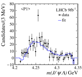
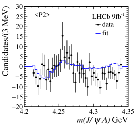
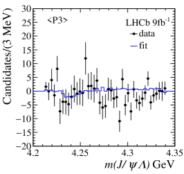
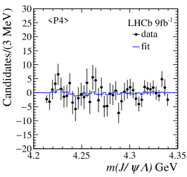
Figure 4: ${P}_{\psi s}^{{\mathchar 28931\relax}}(4338)^{0}$ helicity angular moments as a function of $m({{J\mskip-3.0mu/\mskip-2.0mu\psi}}{\mathchar 28931\relax})$ invariant mass. The black points represent the data while the blue line is the nominal model.

Appendix E Efficiency corrected and background subtracted distributions

The data are assigned weights to account for the efficiency and to subtract the background using the sPlot technique. The efficiency corrected data distributions of $m({\overline{p}}{\mathchar 28931\relax})$, $m({{J\mskip-3.0mu/\mskip-2.0mu\psi}}{\overline{p}})$, $m({{J\mskip-3.0mu/\mskip-2.0mu\psi}}{\mathchar 28931\relax})$ and $\cos{\theta_{K^{*}}}$ are shown in Figure 5. There is a sign difference between this $\cos{\theta_{K^{*}}}$ definition and the one from CMS [16].

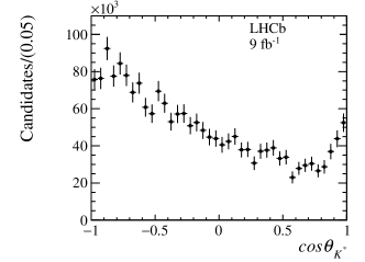
Figure 5: Efficiency corrected and background subtracted distributions for $m({\overline{p}}\Lambda)$, $m(J/\psi{\overline{p}})$, $m(J/\psi\Lambda)$ and $\cos{\theta_{K^{*}}}$.