The Devil in Linear Transformer

Abstract

Linear transformers aim to reduce the quadratic space-time complexity of vanilla transformers. However, they usually suffer from degraded performances on various tasks and corpora. In this paper, we examine existing kernel-based linear transformers and identify two key issues that lead to such performance gaps: 1) unbounded gradients in the attention computation adversely impact the convergence of linear transformer models; 2) attention dilution which trivially distributes attention scores over long sequences while neglecting neighbouring structures. To address these issues, we first identify that the scaling of attention matrices is the devil in unbounded gradients, which turns out unnecessary in linear attention as we show theoretically and empirically. To this end, we propose a new linear attention that replaces the scaling operation with a normalization to stabilize gradients. For the issue of attention dilution, we leverage a diagonal attention to confine attention to only neighbouring tokens in early layers. Benefiting from the stable gradients and improved attention, our new linear transformer model, TransNormer, demonstrates superior performance on text classification and language modeling tasks, as well as on the challenging Long-Range Arena benchmark, surpassing vanilla transformer and existing linear variants by a clear margin while being significantly more space-time efficient. The code is available at TransNormer.

1 Introduction

Transformer models show great performance on a wide range of natural language processing and computer vision tasks Qin et al. (2022); Sun et al. (2022b); Cheng et al. (2022a, b); Zhou et al. (2022). One issue of the vanilla transformer model lies in its quadratic space-time complexity with respect to the input length. Various prior works attempt to alleviate this inefficiency Zaheer et al. (2020); Beltagy et al. (2020); Tay et al. (2020a); Kitaev et al. (2020); Child et al. (2019); Liu et al. (2022); Sun et al. (2022b). In this work, we focus on a particular subset of these methods, known as kernel-based linear transformers Choromanski et al. (2020); Wang et al. (2020); Katharopoulos et al. (2020); Peng et al. (2020); Qin et al. (2022) considering their desirable linear space-time complexity.

Despite their space-time efficiency, linear transformers are not always in favor for practical adoption, largely due to the degraded performance than the vanilla model. To address this issue, we take a close look at existing kernel-based linear transformers and identify two deficiencies that lead to such a performance gap.

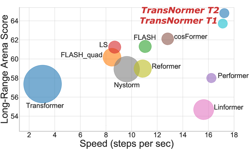
Figure 1: TransNormer has smaller memory footprints (circle sizes) and produces clearly favorable speed (x-axis) and overall scores (y-axis), when evaluated on the challenging Long-Range Arena benchmark than the vanilla transformer and other competing methods.

Unbounded gradients. Most existing linear transformers inherit attention formulation from the vanilla transformer, which scales attention scores to ensure they are bounded within $[0,1]$. However, we theoretically show that such a scaling strategy renders unbounded gradients for linear transformer models. As a result, the unbounded gradients empirically lead to unstable convergence as our preliminary experiments suggest.
Attention dilution. Previous works Titsias (2016); Jang et al. (2016); Gao and Pavel (2017); Qin et al. (2022); Sun et al. (2022b, a) suggest that in vanilla transformer, softmax attention maps tend to be local. In contrast, as shown in Fig 2, we observe that linear transformers often trivially distribute attention scores over the entire sequence even in early layers. Due to this issue, which we refer as attention dilution, important local information is less well preserved in linear models, resulting in inferior performance. This negative impact of attention dilution is also evidenced by the performance drop in our controlled experiments if partly replacing vanilla attention in transformer layers with linear attention ones.

To mitigate these issues, we propose a linear transformer model, called TransNormer, which shows better performance than vanilla transformer on a wide range of task while being significantly faster during runtime, as shown in Fig. 1.

To avoid the unbounded gradients, we introduce NormAttention, which gets rid of scaling over attention matrices while appending an additional normalization only after the attention layer. The choice of the normalization operator is unrestricted, for example, LayerNorm Ba et al. (2016) or RMSNorm Zhang and Sennrich (2019) both serve the purpose. We show empirical results demonstrating that with NormAttention, the gradients are more stable during training, which in turn leads to more consistent convergence.

To alleviate the attention dilution issue, we modify the vanilla attention and allow each token to only attend to its neighbouring tokens, resulting in a diagonal attention. To mimic the behaviors on local semantics of the vanilla transformer, we employ the diagonal attention on early layers while using NormAttention for later ones. In this way, we encourage the model to capture both local and global language context. Note that our diagonal attention can be efficiently computed such that the overall linear space-time complexity of TransNormer is preserved.

We perform extensive experiments on standard tasks, where TransNormer demonstrates lower language modeling perplexities on WikiText-103 and overall higher text classification accuracy on GLUE than vanilla model and other competing methods. In addition, on the challenging Long-Range Arena benchmark, TransNormer also shows favorable results while being faster and more scalable with longer inputs during both training and inference time.

2 Background and related work

We first briefly review vanilla transformer Vaswani et al. (2017) and its efficient variants. The key component of transformers is the self-attention, which operates on query $\mathbf{Q}$, key $\mathbf{K}$ and value $\mathbf{V}$ matrices; each of them is the image of a linear projection taking $\mathbf{X}\in\mathbb{R}^{n\times d}$ as input:

$$\textstyle\begin{gathered}\mathbf{Q}=\mathbf{X}\mathbf{W}_{Q},\mathbf{K}=\mathbf{X}\mathbf{W}_{K},\mathbf{V}=\mathbf{X}\mathbf{W}_{V}\in\mathbb{R}^{n\times d},\end{gathered}$$ (1)

with $n$ the input length, $d$ the hidden dimension. The output $\mathbf{O}\in\mathbb{R}^{n\times d}$ is formulated as:

$$\textstyle\mathbf{O}=\mathrm{Softmax}(\mathbf{Q}\mathbf{K}^{\mkern-1.5mu\mathsf{T}}/\sqrt{d})\mathbf{V},$$ (2)

where the $\mathrm{Softmax}(\cdot)$ step renders quadratic space-time complexity with respect to the input length, making it prohibitive for vanilla transformer to scale to long input sequences. To address this issue, numerous efficient transformers have been explored in the literature. These methods can be generally categorized into two families, i.e., pattern based methods and kernel based methods.

Pattern based methods Zaheer et al. (2020); Beltagy et al. (2020); Tay et al. (2020a); Kitaev et al. (2020); Child et al. (2019) sparsify the attention calculation with handcrafted or learnable masking patterns. Kernel-based methods adopt kernel functions to decompose softmax attention, which reduces the theoretical space-time complexity to linear. In this paper, we refer the kernel-based variants as linear transformers for simplicity.

In the kernel-based methods Choromanski et al. (2020); Katharopoulos et al. (2020); Peng et al. (2020); Qin et al. (2022); Zheng et al. (2022); Wang et al. (2020), a kernel function $\phi(\cdot)$ maps queries and keys to their hidden representations. Then the output of the linear attention can be rewritten as:

$$\mathbf{O} =\mathbf{\Delta}^{-1}\phi(\mathbf{Q})[\phi(\mathbf{K})^{\mkern-1.5mu\mathsf{T}}\mathbf{V}],$$ (3)

$$\mathbf{\Delta} =\mathrm{diag}(\phi(\mathbf{Q})[\phi(\mathbf{K})^{\mkern-1.5mu\mathsf{T}}{\mathbf{1}}_{n}]).$$

where the product of keys and values are computed to avoid the quadratic $n\times n$ matrix. Existing methods mainly differ in the design of kernel functions. For example, Choromanski et al. (2020) and Katharopoulos et al. (2020) adopt activation function $1+elu$ to process query and key. Wang et al. (2020) assumes attention matrices are low-rank. Peng et al. (2020) and Zheng et al. (2022) approximate softmax under constrained theoretical bounds. Qin et al. (2022) propose a linear alternative to the attention based on empirical properties of the softmax function.

These methods focus on either approximating or altering the softmax operator while preserving its properties. Compared with the vanilla transformer, these methods often trade performance for efficiency, usually resulting in worse task performance. In this paper, we argue that there are two essential reasons leading to such a performance gap, discussed in detail as follows.

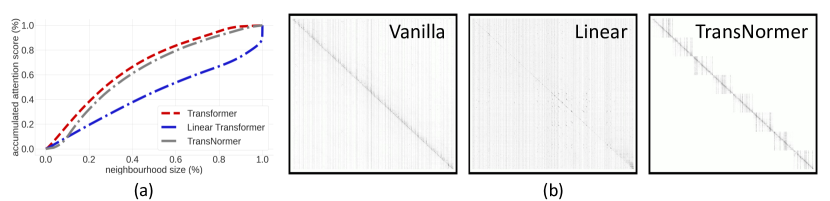
Figure 2: (a): Comparison of locally accumulated attention scores of different transformer variants. The x-axis denotes ratio of neighbourhood size relative to the input length; the y-axis denotes accumulated attention scores inside this neighbourhood for the centering token. The curve for the vanilla transformer model increases more sharply, indicating that the attention scores are more concentrated. Our model greatly alleviates the attention dilution issue for linear models. (b): Qualitative comparison of attention matrices in early model layers. The proposed TransNormer produces more similar patterns to the original vanilla transformer, benefiting to better capture local-global language context, while the linear model suffers clearly from the issue of attention dilution and gets distracted by distant tokens in early layers.

3 The devil in linear attention

In this section, we motivate the design principles of TransNormer by providing theoretical evidence for the unbounded gradients, and empirical results showing the adverse influence of attention dilution.

3.1 Unbounded gradients

Few work on linear transformers analyzes their gradients during training. Our first key observation is that kernel-based linear attention suffer from unbounded gradients, causing unstable convergence during training. In the following, we highlight the main theoretical results while referring readers to Appendix D for the full derivation.

Consider a self-attention module, either vanilla or linear attention. Its attention matrix $\mathbf{P}\in\mathbb{R}^{n\times n}$ can be represented in the following unified form :

$$p_{ij}=\frac{f(s_{ij})}{\sum_{k=1}^{n}f(s_{ik})},f:\mathbb{R}\to\mathbb{R}.$$ (4)

Vanilla and linear attention differ mainly in their computation of token-wise similarities $s_{ij}$. In vanilla attention, $s_{ij}$ is computed as:

$$s_{ij}=\mathbf{q}_{i}^{\mkern-1.5mu\mathsf{T}}\mathbf{k}_{j}/\sqrt{d},f(x)=\exp(x),$$ (5)

while for linear attentions, $s_{ij}$ can be decomposed using a kernel function $\phi$, such that:

$$s_{ij}=\phi(\mathbf{q}_{i})^{\mkern-1.5mu\mathsf{T}}\phi(\mathbf{k}_{j}),f(x)=x.$$ (6)

Given the above definitions, the gradients of the attention matrix $\mathbf{P}$ is derived as:

$$\frac{\partial p_{ij}}{\partial s_{ik}}=\frac{f^{\prime}(s_{ik})}{f(s_{ik})}\left(1_{j=k}p_{ij}-p_{ij}p_{ik}\right)$$ (7)

Therefore, for the vanilla attention, the partial derivative $\frac{\partial p_{ij}}{\partial s_{ik}}$ is:

$$f^{\prime}(x) =\exp(x)=f(x)$$ (8)

$$\frac{\partial p_{ij}}{\partial s_{ik}} =1_{j=k}p_{ij}-p_{ij}p_{ik}$$

$$=\begin{cases}p_{ik}-p_{ik}p_{ik}\in[0,1/4]&j=k\\ -p_{ij}p_{ik}\in[-1/4,0]&j\neq k\end{cases}$$

and it is bounded as:

$$\left|\frac{\partial p_{ij}}{\partial s_{ik}}\right|\leq\frac{1}{4}.$$ (9)

However, for linear attentions, we have:

$$f^{\prime}(x) =1$$ (10)

$$\frac{\partial p_{ij}}{\partial s_{ik}} =\frac{1}{s_{ik}}\left(1_{j=k}p_{ij}-p_{ij}p_{ik}\right)$$

$$=\begin{cases}\frac{1}{s_{ik}}\left(p_{ik}-p_{ik}p_{ik}\right)&j=k\\ \frac{1}{s_{ik}}(-p_{ij}p_{ik})&j\neq k\end{cases}$$

and

$$\left|\frac{\partial p_{ij}}{\partial s_{ik}}\right|\leq\frac{1}{4|s_{ik}|}.$$ (11)

Since $|s_{ik}|^{-1}=|\phi(\mathbf{q}_{i})\phi(\mathbf{k}_{j})^{\mkern-1.5mu\mathsf{T}}|^{-1}$ can be arbitrarily large, the gradient of linear attention has no upper bound. On the other hand, we can also show that the gradient of linear attention has no lower bound:

Proposition 3.1.

$\forall M>0$, there exists $\mathbf{q}_{i},\mathbf{k}_{j}\in\mathbb{R}^{d},j=1,\ldots,n$, such that:

$$\left|\frac{\partial p_{ij}}{\partial s_{ik}}\right|>M.$$ (12)

The unbounded gradients lead to less stable optimization and worse convergence results in our preliminary studies.

3.2 Attention dilution

It is a known property of vanilla attention to emphasize on neighbouring tokens  Titsias (2016); Qin et al. (2022). However, this property does not directly inherit to the linear transformer variants.

To quantify the attention dilution issue, we introduce a metric called locally accumulated attention score, which measures how much attention scores are distributed within the local neighbourhood of a particular token.

For an input sequence of length $N$, consider a local neighbourhood $\{x_{start},...,x_{i}...,x_{end}\}$ centering around token $x_{i}$ of total length $r\cdot N$, with $r$ the ratio relative to the total input, the locally accumulated attention score for token $x_{i}$ is defined as $l(i,r,N)=p_{i,start}+...+p_{i,end}$. A higher score indicates the particular attention layer concentrates on the local neighbourhood, while a lower score tends to indicate the issue of attention dilution, where scores are distributed more evenly to local and distant tokens. For example, $l(i,0.4,N)=0.6$ means that that 40% of the neighbors around $i$’th token contribute 60% of the attention score.

In Fig. 2 (a), we compare locally accumulated attention scores (y-axis) for vanilla transformer and linear transformer, with varying sizes of neighbourhood by ratio (x-axis). We show the average score over each position across the entire sequence. It can be seen that the area under the vanilla model curve is significantly larger than that of the linear model. This provides evidence that the vanilla attention is more concentrated locally, while the linear transformer suffers from the issue of attention dilution. This is further qualitatively supported by Fig. 2 (b), where the attention maps for vanilla model are more concentrated than the linear model.

4 Method

Based on the aforementioned observations, we propose a new linear transformer network called TransNormer that addresses the above two limitations of current linear transformers. The overall architecture is shown in Fig. 3.

4.1 The overall architecture

Vanilla attention suffers less in attention dilution while linear attention is more efficient and scalable on longer sequences. This motivate us to design a method that exploits the best of the both worlds by using these mechanisms in combined.

Specifically, our network consists of two types of attention: DiagAttention for the early stage of the model and NormAttention for the later stage. The former addresses the attention dilution issue and the later aims to stabilize training gradients. Note that by properly reshaping the inputs, the diagonal attention can be efficiently computed in linear space-time, thus preserving the overall linear complexity.

4.2 NormAttention

Table 1: Ablation of linear attention with scaling operation. Directly removing scaling operation i.e., the denominator in Eq. 4, leads to significant performance drop. Our normalization strategy achieves better result.

method	ppl(val)
$1+elu$	4.98
$1+elu$ w/o scaling	797.08
NormAttention	4.94

As proved in Sec. 3, the scaling operation, i.e., the denominator in Eq. 4, in the linear transformers hinder the optimization due to the unbounded gradients. To solve this issue, we propose to remove the scaling operation in the linear transformers. However, as shown in Table. 1, directly removing the scaling operation leads to critical performance drop since the attention map becomes unbounded in the forward pass. Therefore, an alternative is required to bound both attention maps during forward and their gradients during backward passes in linear attentions.

Our proposed solution is simple yet effective. Given a linear attention, the attention without scaling can be formulated as:

$$\mathbf{O}=\mathbf{Q}(\mathbf{K}^{\mkern-1.5mu\mathsf{T}}\mathbf{V}).$$ (13)

We empirically find that we can apply an arbitrary normalization on this attention to bound it, which leads to our NormAttention as:

$$\mathbf{O}_{\text{norm}}=\mathrm{XNorm}(\mathbf{Q}(\mathbf{K}^{\mkern-1.5mu\mathsf{T}}\mathbf{V})),$$ (14)

where the $\mathrm{XNorm}$ can be Layernorm(Ba et al., 2016) or RMSNorm (Zhang and Sennrich, 2019) and etc. We use the RMSNorm in our experiments as it is slightly faster than other options.

It can be proved that the gradients of NormAttention is bounded by:

$$\left|\frac{\partial\mathcal{L}}{\partial s_{ij}}\right|\leq\frac{3c_{1}c_{2}d}{2\sqrt{\epsilon}}<\infty,$$ (15)

where $\mathcal{L}$ is the loss function, $\epsilon$ is the small constant that used in RMSNorm, $d$ is the embedding dimension and

$$c_{1} =\max_{i=1}^{n}\|\nabla_{\mathbf{O}_{i}}\mathcal{L}\|_{2}<\infty$$ (16)

$$c_{2} =\max_{i=1}^{n}\|\mathbf{V}_{i}\|_{2}<\infty$$

To demonstrate the gradients stability of the NormAttention, we compare the relative standard deviation of gradients during each training iterations to other linear transformers and vanilla transformer. Specifically, we train our model for 50k iterations with RoBERTa architecture on the WikiText103 Merity et al. (2017) and obtain the relative standard deviation of all iterations’ gradients. As shown in Table 2, existing linear methods Choromanski et al. (2020); Katharopoulos et al. (2020) have substantially higher deviations compared to vanilla attention, which leads to inferior results. The NormAttention produces more stable gradients, which validates the effectiveness of our method.

Table 2: Relative standard deviation of training gradients over 50k iterations. Our proposed NormAttention provides more stable gradients which are closer to vanilla transformer.

method	Relative Standard Deviation
$1+elu$ Katharopoulos et al. (2020)	0.58
PerformerChoromanski et al. (2020)	0.47
VanillaVaswani et al. (2017)	0.25
NormAttention	0.20

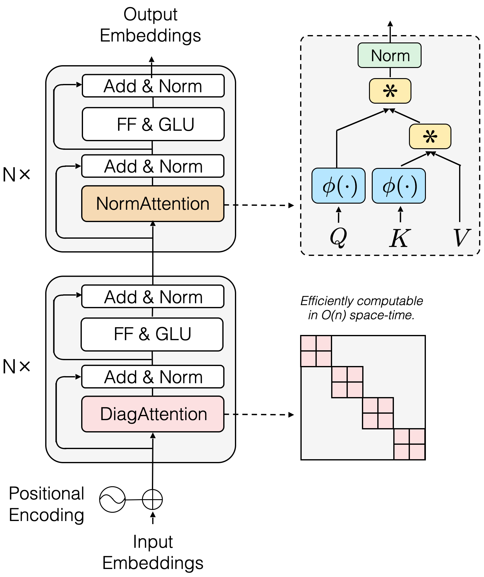
Figure 3: Architecture overview of the proposed TransNormer. In the early stages, we leverage DiagAttention, where attention is only calculated inside the blocks to enforce neighbouring focus. In late stages, NormAttention assists to obtain a more stable gradients in linear complexity.

4.3 DiagAttention

To better understand the design principles, we show in Table 3 that by replacing partial layers of linear transformers with vanilla attention, the performance on language modeling is evidently improved. The results also suggest that capturing more local information in early layers are more helpful than otherwise.

Table 3: Ablation on attention dilution issue. We implement all structures under the same setting: Vanilla Vaswani et al. (2017), $1+elu$ Katharopoulos et al. (2020).

Early layers	Later layers	ppl (val)
$1+elu$	$1+elu$	4.98
$1+elu$	Vanilla	3.90
Vanilla	$1+elu$	3.76

To this end, we leverage none-overlapped block-based strategy to reduce the space-time complexity of the vanilla attention. Based on the observation in Fig. 2, we utilize a strict diagonal blocked pattern to constraint the attention in a certain range. Since the attentions are calculated inside each block, the computation complexity of our diagonal attention is $O(nwd)$, where $n$ is sequence length , $w$ is the block size and $d$ is feature dimension. When $d\ll n$, the complexity scales linearly respect to the sequence length $n$. In subsequent sections, we use DiagAttention to refer to Diagonal attention.

We empirically find that applying DiagAttention to the later stages of a model hurts the performance as shown in Table. 9. It indicates that the model requires a global field of view in the later layers, which also justifies our choices of NormAttention in later layers of TransNormer.

5 Experiments

In this section, we compare our method to other linear transformers and the vanilla transformer on autoregressive language modeling, bidirectional language modeling as well as the Long Range Arena benchmark (Tay et al., 2020b). We also provide an extensive ablation study to vindicate our choice in designing the TransNormer.

We validate our method on two variants of the TransNormer. The TransNormer T1 uses the ReLA attention (Zhang et al., 2021) in the DiagAttention and the elu as the activation function in the NormAttention. The TransNormer T2 uses the $\mathtt{Softmax}$ attention (Vaswani et al., 2017) in the DiagAttention and the 1+elu as the activation function in the NormAttention.

For experiments, we first study the autoregressive language modeling on WikiText-103 (Merity et al., 2017) in section 5.2. Then in section 5.2 we test our method on bidirectional language modeling, which is pre-trained on WikiText-103 (Merity et al., 2017) and then fine-tuned on several downstream tasks from the GLUE benchmark (Wang et al., 2018). Finally, we test TransNormer on the Long-Range Arena benchmark (Tay et al., 2020b) to evaluate its ability in modeling long-range dependencies and efficiencies in section 5.2.

5.1 Settings

We implement our models in the Fairseq framework (Ott et al., 2019) and train them on 8 V100 GPUS. We use the same training configuration for all competitors and we list detailed hyper-parameters in Appendix F. We choose the FLASH-quad, FLASH (Hua et al., 2022), Transformer-LS (Zhu et al., 2021), Performer (Choromanski et al., 2020), 1+elu (Katharopoulos et al., 2020) as our main competing methods.

For the autoregressive language modeling, we use 6 decoder layers (10 layers for the FlASH/FLASH-quad) as our base model and all models are trained on the WikiText-103 dataset (Merity et al., 2017) for 100K steps with a learning rate of $0.005$. We use the perplexity (PPL) as the evaluation metric.

For the bidirectional language modeling, we choose the RoBERTa base (Liu et al., 2019) for all methods. It consists of 12 encoder layers (24 layers for the FLASH and FLASH-quad to match the number of parameters). All models are pre-trained on the WikiText-103 (Merity et al., 2017) for 50K steps with lr=0.005 and fine-tuned on the GLUE dataset (Wang et al., 2018). We use different learning rates among 1e-5, 3e-5, 6e-5, 1e-4 and choosing the best result after fine-tuning for 3 epochs.

For the Long-Range Arena benchmark, to make sure it reflect the practical speed in Pytorch platform, we re-implement the benchmark in Pytorch. We adopt the same configuration from the Skyformer Chen et al. (2021) and make sure all models have a similar parameter size. We use the same training hyper parameters for all models as well.

Table 4: Quantitative results in autoregressive language modeling. The best result is highlighted with bold and the second with underlined. The smaller the better for the PPL metric. LS stands for transformer-LS.

Method	PPL (val)	PPL (test)	Params (m)
Vanilla	29.63	31.01	156.00
LS	32.37	32.59	159.46
FLASH-quad	31.88	33.50	153.51
FLASH	33.18	34.63	153.52
1+elu	32.63	34.25	156.00
Performer	75.29	77.65	156.00
TransNormer T1	29.89	31.35	155.99
TransNormer T2	29.57	31.01	155.99

Table 5: Quantitative results of the GLUE benchmark. MNLI is reported by the match/mismatch splits. MRPC is reported by F1 score. CoLA is reported by Matthews correlation coefficient. All the other tasks are measured by the accuracy. LS stands for transformer-LS. The best result is highlighted with bold and the second with underlined. The larger the better for all metrics. "-" means unconverged.

Method	MNLI	QNLI	QQP	SST-2	MRPC	CoLA	AVG	Params (m)
Vanilla	79.37/79.07	87.79	88.04	90.25	88.35	38.63	78.79	124.70
FLASH-quad	78.71/79.43	86.36	88.95	90.94	81.73	41.28	78.20	127.11
FLASH	79.45/80.08	87.10	88.83	90.71	82.50	29.40	76.87	127.12
LS	77.01/76.78	84.86	86.85	90.25	82.65	40.65	77.01	128.28
Performer	58.85/59.52	63.44	79.10	81.42	82.11	19.41	63.41	124.70
1+elu	74.87/75.37	82.59	86.9	87.27	83.03	-	70.00	124.0
TransNormer T1	79.06/79.93	87.00	88.61	91.17	84.50	45.38	79.38	124.67
TransNormer T2	77.28/78.53	85.39	88.56	90.71	85.06	45.90	78.78	124.67

Table 6: Quantitative results on the Long-Range Arena benchmark. The best result is highlighted with bold and the second with underlined. The larger the better for all metrics.

Model	Text	ListOps	Retrieval	Pathfinder	Image	AVG.
Transformer	61.95	38.37	80.69	65.26	40.57	57.37
Kernelized Attention	60.22	38.78	81.77	70.73	41.29	58.56
Nystromformer	64.83	38.51	80.52	69.48	41.30	58.93
Linformer	58.93	37.45	78.19	60.93	37.96	54.69
Informer	62.64	32.53	77.57	57.83	38.10	53.73
Performer	64.19	38.02	80.04	66.30	41.43	58.00
Reformer	62.93	37.68	78.99	66.49	48.87	58.99
BigBird	63.86	39.25	80.28	68.72	43.16	59.05
Skyformer	64.70	38.69	82.06	70.73	40.77	59.39
LS	66.62	40.30	81.68	69.98	47.60	61.24
cosFormer	67.70	36.50	83.15	71.96	51.23	62.11
FLASH-quad	64.10	42.20	83.00	63.28	48.30	60.18
FLASH	64.10	38.70	86.10	70.25	47.40	61.31
TransNormer T1	66.90	41.03	83.11	75.92	51.60	63.71
TransNormer T2	72.20	41.60	83.82	76.80	49.60	64.80

5.2 Results

Autoregressive language modeling

We report the results in Table 4. It can be found that both TransNormer variants get comparable or better perplexity to the vanilla attention and outperform all existing linear models with a clear margin. For example, compared to previous state-of-the-art linear methods on validation setHua et al. (2022) and test setZhu et al. (2021), TransNormer T2 achieves substantially lower perplexity by 2.31 and 1.58 respectively. It demonstrates the effectiveness of our method in causal models.

Table 7: Speed comparison on Long-Range Arena benchmark. We mark it with a dash if a method exhausts GPU memory. The higher the better for all metrics. The 1K,…,5K represent the input sequence length.

	Inference Speed(steps per sec)					Train Speed(steps per sec)
model	1K	2K	3K	4K	5K	1K	2K	3K	4K	5K
Transformer	39.06	10.05	-	-	-	15.34	3.05	-	-	-
FLASH-quad	44.64	16.45	9.40	6.54	5.39	19.84	8.47	5.19	3.59	2.92
FLASH	40.32	23.15	16.89	14.04	13.16	20.49	11.06	8.47	7.23	6.93
LS	32.05	17.36	12.14	10.16	9.06	15.43	8.68	6.28	5.24	4.76
Performer	104.17	56.82	42.37	33.78	31.25	28.41	16.23	12.02	10.04	9.06
cosFormer	86.21	46.30	32.47	27.47	25.00	22.94	12.82	9.19	7.79	7.14
Linformer	104.17	58.14	40.32	31.25	26.32	27.17	15.63	11.26	8.77	7.42
Reformer	78.13	38.46	26.04	19.84	16.23	20.16	10.87	7.46	5.69	4.70
Nystorm	58.14	38.46	29.07	23.81	20.33	14.12	9.62	7.46	6.11	5.26
TransNormer T1	113.64	65.79	46.30	39.06	35.71	28.41	17.12	12.76	10.87	10.12
TransNormer T2	119.05	65.79	47.17	39.68	36.23	29.41	17.24	12.95	10.96	10.16

Bidirectional language modeling

We show our bidirectional results on the GLUE benchmark in Table. 5. Our method achieves superior performance to all the competing methods in average. On three tasks, i.e., SST-2, MRPC, CoLA, TransNormer reports comprehensively better results than all competing linear methods, such as 4.62 higher on CoLA. Further, one of our variants i.e., TransNormer T1, even outperforms the vanilla attention with a notable margin. It proves the effectiveness of our method in bidirectional language modeling.

Long Range Arena Benchmark

The results before the transformer Long-short (abbr. LS) are taken from the Skyformer Chen et al. (2021). As shown in Table. 6, we achieve either first or second places across all five tasks. In terms of overall results, both TransNormer variants (T1,T2) outperform all other competing methods including vanilla transformer Vaswani et al. (2017), which validates our capability to encode long sequences.

5.3 Speed comparison

We compare the training and inference speed of the TransNormer with other methods. For a fair and comprehensive comparison, we follow exactly the same configurations of the SkyformerChen et al. (2021) and report step per second under different sequence lengths. Timing is conducted on a Nvidia A6000 GPU with 48G GPU memory. Table. 7 suggests that the vanilla transformer is substantially slow and exhausts GPU memory with sequence longer than 3k. Compared to other efficient transformers, our TransNormer achieves faster speed with comparable GPU memory footprints, while competing efficient methods all report worse results compared to our TransNormer. For instance, compared to FLASH-quad Hua et al. (2022) that achieves previous best linear results on both autoregressive and bidirectional benchmarks, our model performs over 300% faster during training and 150% faster during inference.

5.4 Ablation study

In this section, we justify our design choice of the TransNormer, including , the selection of the FFN module, and the size of the attention block in DiagAttention. We use the PPL from the Roberta pre-training stage as our evaluation metric.

Structure design

Table 8: Ablation of the proportion of the attentions. We empirically find that the balanced structure achieves the best result. We abbreviate the DiagAttention as BlockAtt and NormAttention as NormAtt.

Early stage BlockAtt	Later stage NormAtt	T1 ppl(val)	T2 ppl(val)
0	12	4.23	4.48
3	9	4.13	3.83
6	6	3.82	3.81
9	3	3.87	3.86
12	0	4.75	4.66

Table 9: Ablation of the order of two proposed attention. Using DiagAttention in the early stage achieves better results than using it on later stage.

Early stage	Later stage	T1 ppl(val)	T2 ppl(val)
NormAtt	BlockAtt	4.13	4.21
BlockAtt	NormAtt	3.82	3.81

As aforementioned, we empirically choose the first 6 layers as the early stage of the model and the rest as the later stage. We provide the designing ground for this choice in Table. 8. It can be also observed that either choosing the DiagAttention or NormAttention for the entire model will lead to inferior performance. We also provide the ablation results of swapping the order of the DiagAttention and the NormAttention in Table. 9. Using DiagAttention in the early stage achieves significantly better results than using it on later stage. It further proves our claim that the early stage focuses on neighbouring tokens while the later stage needs long-range attentions.

FFN module

Table 10: Ablation of the selection of the FFN modules. The GLU leads to better results.

FFN type	T1 ppl(val)	T2 ppl(val)
FFN	3.93	3.93
GLU(ours)	3.82	3.81

We ablate the selection of the FFN modules in Table. 10. Compared with the traditional FFN (Vaswani et al., 2017), the GLU (Shazeer, 2020) achieves better results.

Block size

Table 11: Ablation of on block sizes in the DiagAttention. The larger block size the better results.

Block size	T1 ppl(val)	T2 ppl(val)
32	3.92	3.90
64	3.82	3.81
128	3.72	3.69

From the Table. 11, we observe clear performance improvements with increased block sizes. However, since the complexity of the DiagAttention is $O(nwd)$, larger block size $w$ leads to heavier computational overhead. We choose a block size as 64 as a trade-off between performance and computational cost.

Combination of attentions

Finally, we study the effect that whether we should use both attentions in one layer. In particular, we compare either to 1) use DiagAttention and NormAttention sequentially in a layer with different orders; or to 2) use them in parallel in each attention layer and then concatenate their embedding output. Table. 12 shows that we should not use these attentions sequentially within a layer and apply them in parallel will double the computation complexities without improving the performance.

Table 12: Ablation of the combination of two proposed attention. In first two rows, the two attention layers appear in an interleaved manner. D for the DiagAttention and N for the NormAttention.

approach	T1 ppl(val)	T2 ppl(val)
altering D$\rightarrow$N	4.19	4.23
altering N$\rightarrow$D	4.11	4.21
parallel	3.77	3.82
TransNormer	3.82	3.81

6 Conclusion

In this paper, we identified two key issues that cause the inferior performance of existing linear transformer models: 1) unbounded gradients; 2) attention dilution. For the former issue, we proposed a new NormAttention to stabilize the training gradients. For the latter, we develop DiagAttention to force the model concentrate attention in neighbouring tokens. The resultant model TransNormer marries the strength of the vanilla transformers and the linear transformers, outperforming competing linear transformers on both autoregressive and bidirectional language modeling, text classification tasks and the challenging Long-range arena benchmark.

Limitations

In this paper, we identified two main issues of current linear transformers and provided a comprehensive analysis in natural language processing tasks. However, with the booming development of vision transformers, whether they share the same issues of linear NLP transformers is yet to be discovered. We will validate our method on the linear vision transformers in our future work.

Ethics Statement

The proposed technique is beneficial to develop large-scale environment-friendly language models by reducing computing resource demand. Corpus used to train the model is from public web sources, which may contain biased, explicit or improper content. Further assessment and regulation have to be in-place before deploying the model in practice.

Appendix

Appendix A Mathematical Notations

We use bold uppercase letters for matrices($\mathbf{M}$), bold lowercase letters for vectors($\mathbf{m}$), and lowercase letters for scalars($m_{ij}$). We represent all vectors as column vectors and denote the $i$th row of matrix $\mathbf{M}$ by $\mathbf{m}_{i}^{\top}$ or $\mathbf{M}_{i}$. We use $\|.\|_{2}$ to denote the $l_{2}$ norm and $\|.\|_{F}$ to denote the Frobenius norm of the matrix and the vector.

The main mathematical symbols are input $\mathbf{X}\in\mathbb{R}^{n\times d}$, $\mathbf{Q}$ (Query), $\mathbf{K}$ (Key) and $\mathbf{V}$ (Value), which has the following form:

$$\mathbf{X} =\left[\begin{matrix}\mathbf{x}_{1}^{\mkern-1.5mu\mathsf{T}}\\ \vdots\\ \mathbf{x}_{n}^{\mkern-1.5mu\mathsf{T}}\end{matrix}\right]\in\mathbb{R}^{n\times d},$$ (17)

$$\mathbf{Q} =\left[\begin{matrix}\mathbf{q}_{1}^{\mkern-1.5mu\mathsf{T}}\\ \vdots\\ \mathbf{q}_{n}^{\mkern-1.5mu\mathsf{T}}\end{matrix}\right]=\mathbf{XW}_{Q}=\left[\begin{matrix}\mathbf{x}_{1}^{\mkern-1.5mu\mathsf{T}}\mathbf{W}_{Q}\\ \vdots\\ \mathbf{x}_{n}^{\mkern-1.5mu\mathsf{T}}\mathbf{W}_{Q}\end{matrix}\right]\in\mathbb{R}^{n\times d},$$

$$\mathbf{K} =\left[\begin{matrix}\mathbf{k}_{1}^{\mkern-1.5mu\mathsf{T}}\\ \vdots\\ \mathbf{k}_{n}^{\mkern-1.5mu\mathsf{T}}\end{matrix}\right]=\mathbf{XW}_{K}=\left[\begin{matrix}\mathbf{x}_{1}^{\mkern-1.5mu\mathsf{T}}\mathbf{W}_{K}\\ \vdots\\ \mathbf{x}_{n}^{\mkern-1.5mu\mathsf{T}}\mathbf{W}_{K}\end{matrix}\right]\in\mathbb{R}^{n\times d},$$

$$\mathbf{V} =\left[\begin{matrix}\mathbf{v}_{1}^{\mkern-1.5mu\mathsf{T}}\\ \vdots\\ \mathbf{v}_{n}^{\mkern-1.5mu\mathsf{T}}\end{matrix}\right]=\mathbf{XW}_{V}=\left[\begin{matrix}\mathbf{x}_{1}^{\mkern-1.5mu\mathsf{T}}\mathbf{W}_{V}\\ \vdots\\ \mathbf{x}_{n}^{\mkern-1.5mu\mathsf{T}}\mathbf{W}_{V}\end{matrix}\right]\in\mathbb{R}^{n\times d},$$

where $\mathbf{W}_{Q},\mathbf{W}_{K},\mathbf{W}_{V}\in\mathbb{R}^{d\times d}$.

Appendix B Proof of gradients’ upper bound

In this part, we will proof the bound in (8) and (10), all we need to prove is:

$$0\leq p_{ik}(1-p_{ik})\leq\frac{1}{4},0\leq p_{ij}p_{ik}\leq\frac{1}{4}.$$ (18)

We adopt the theorem that geometric mean is bounded by arithmetic mean, i.e.,

$$\sqrt{ab}\leq\frac{a+b}{2}\Longleftrightarrow ab\leq\left(\frac{a+b}{2}\right)^{2},\forall a,b\geq 0.$$ (19)

We take $a=p_{ik},b=1-p_{ik}$ to complete the proof. The first bound can be proven by:

$$0\leq p_{ik}(1-p_{ik})\leq\left(\frac{p_{ik}+1-p_{ik}}{2}\right)^{2}=\frac{1}{4}.$$ (20)

For the second bound, we first use the fact that:

$$0\leq p_{ij}+p_{ik}\leq 1\Rightarrow p_{ij}\leq 1-p_{ik}.$$ (21)

So we have:

$$0\leq p_{ij}p_{ik}\leq(1-p_{ik})p_{ik}\leq\frac{1}{4}.$$ (22)

Appendix C Proof of Proposition 3.1

Proof of Proposition 3.1.

$\forall\epsilon>0$ and kernel function $\phi$, let:

$$\begin{gathered}\mathbf{q}_{i}=\mathbf{k}_{j}=\phi^{-1}(\mathbf{x}_{0}),\\ 0<\|\mathbf{x}_{0}\|_{2}\leq\sqrt{\epsilon},i,j=1,\ldots,n.\end{gathered}$$ (23)

Then

$$\phi(\mathbf{q}_{i})=\phi(\mathbf{k}_{j})=\mathbf{x}_{0},i,j=1,...,n.$$ (24)

So

$$s_{ij}=\phi(\mathbf{q}_{i})^{\mkern-1.5mu\mathsf{T}}\phi(\mathbf{k}_{j})={\mathbf{x}_{0}}^{\mkern-1.5mu\mathsf{T}}{\mathbf{x}_{0}}\in(0,\epsilon],$$ (25)

and

$$p_{ij}=\frac{s_{ij}}{\sum_{k=1}^{n}s_{ik}}=\frac{{\mathbf{x}_{0}}^{\mkern-1.5mu\mathsf{T}}{\mathbf{x}_{0}}}{\sum_{k=1}^{n}{\mathbf{x}_{0}}^{\mkern-1.5mu\mathsf{T}}{\mathbf{x}_{0}}}=\frac{1}{n}.$$ (26)

According to (10), we have:

$$\frac{\partial p_{ij}}{\partial s_{ik}} =\begin{cases}\frac{1}{{\mathbf{x}_{0}}^{\mkern-1.5mu\mathsf{T}}{\mathbf{x}_{0}}}\frac{1}{n}(1-\frac{1}{n})&j=k\\ -\frac{1}{{\mathbf{x}_{0}}^{\mkern-1.5mu\mathsf{T}}{\mathbf{x}_{0}}}\frac{1}{n^{2}}&j\neq k\end{cases},$$ (27)

$$\left|\frac{\partial p_{ij}}{\partial s_{ik}}\right| =\begin{cases}\frac{1}{{\mathbf{x}_{0}}^{\mkern-1.5mu\mathsf{T}}{\mathbf{x}_{0}}}\frac{1}{n}(1-\frac{1}{n})&j=k\\ \frac{1}{{\mathbf{x}_{0}}^{\mkern-1.5mu\mathsf{T}}{\mathbf{x}_{0}}}\frac{1}{n^{2}}&j\neq k\end{cases}$$

$$\geq\begin{cases}\frac{1}{\epsilon n}(1-\frac{1}{n})&j=k\\ \frac{1}{\epsilon n^{2}}&j\neq k\end{cases}.$$

Let $\epsilon\to 0^{+}$, then $\frac{1}{\epsilon n^{2}},\frac{1}{\epsilon n}(1-\frac{1}{n})\to\infty$, so $\left|\frac{\partial p_{ij}}{\partial s_{ik}}\right|\to\infty$.

∎

Appendix D Analyze the gradient of each method

In this section, let’s consider a one-layer Transformer, for a multi-layer Transformer, we can prove our conclusion using induction.

We begin this section by introducing some mathematical notations.

D.1 Notations

In vanilla attention, we have:

$$\mathbf{S} =\mathbf{Q}\mathbf{K}^{\mkern-1.5mu\mathsf{T}}\in\mathbb{R}^{n\times n},$$ (28)

$$\mathbf{P} =\mathrm{Softmax}(\mathbf{S})\in\mathbb{R}^{n\times n},$$

$$\mathbf{O} =\mathbf{P}\mathbf{V}\in\mathbb{R}^{n\times d}.$$

In linear attention, we have:

$$\mathbf{S} =\phi(\mathbf{Q})\phi(\mathbf{K})^{\mkern-1.5mu\mathsf{T}}\in\mathbb{R}^{n\times n},$$ (29)

$$\mathbf{\Delta} =\mathrm{diag}(\mathbf{S}{\mathbf{1}}_{n})\in\mathbb{R}^{n\times n},$$

$$\mathbf{P} =\mathbf{\Delta}^{-1}\mathbf{S}\in\mathbb{R}^{n\times n},$$

$$\mathbf{O} =\mathbf{P}\mathbf{V}\in\mathbb{R}^{n\times d}.$$

Although this term is not calculated in linear attention, we discuss it conceptually. Note that the above formulations can be unified into the following form :

$$\mathbf{S} =f(\psi(\mathbf{Q})\psi(\mathbf{K})^{\mkern-1.5mu\mathsf{T}})\in\mathbb{R}^{n\times n},$$ (30)

$$\mathbf{\Delta} =\mathrm{diag}(\mathbf{S}{\mathbf{1}}_{n})\in\mathbb{R}^{n\times n},$$

$$\mathbf{P} =\mathbf{\Delta}^{-1}\mathbf{S}\in\mathbb{R}^{n\times n},$$

$$\mathbf{O} =\mathbf{P}\mathbf{V}\in\mathbb{R}^{n\times d},$$

where in vanilla attention, we have:

$$\psi(\mathbf{x})=\mathbf{x},f(x)=\exp(x),$$ (31)

and in linear attention, we have:

$$\psi(\mathbf{x})=\phi(\mathbf{x}),f(x)=x.$$ (32)

In NormAttention, we have:

$$\mathbf{S} =\phi(\mathbf{Q})\phi(\mathbf{K})^{\mkern-1.5mu\mathsf{T}}\in\mathbb{R}^{n\times n},$$ (33)

$$\mathbf{T} =\mathbf{S}\mathbf{V}\in\mathbb{R}^{n\times d},$$

$$\mathbf{O} =\mathrm{RMSNorm}(\mathbf{T})$$

$$\triangleq\left[\begin{matrix}\mathrm{RMSNorm}(\mathbf{t}_{1})^{\mkern-1.5mu\mathsf{T}}\\ \vdots\\ \mathrm{RMSNorm}(\mathbf{t}_{n})^{\mkern-1.5mu\mathsf{T}}\end{matrix}\right]\in\mathbb{R}^{n\times d},$$

where $\mathrm{RMSNorm}$ is defined as follows:

Definition D.1.

$$\mathrm{RMSNorm}(\mathbf{x}) =\frac{\mathbf{x}}{\sqrt{\sigma^{2}+\epsilon}},$$ (34)

$$\sigma^{2} =\frac{\sum_{i=1}^{d}x_{i}^{2}}{d},$$

$$\epsilon >0,$$

$$\mathbf{x} \in\mathbb{R}^{d}.$$

In the subsequent discussion, we define gradient $\nabla_{\mathbf{M}}\mathcal{L}$ as:

Definition D.2.

$$[\nabla_{\mathbf{M}}\mathcal{L}]_{ij}=\frac{\partial\mathcal{L}}{\partial m_{ij}},$$ (35)

where $\mathcal{L}$ stands for loss function, $\mathbf{M}$ is a parameter matrix.

Then we define the mapping $h$ as:

Definition D.3.

$$\begin{gathered}h:\mathbb{R}^{n\times m}\to\mathbb{R},h(\mathbf{X})=\max_{i=1}^{n}\|\mathbf{X}_{i}\|_{2},\\ \mathbf{X}\in\mathbb{R}^{n\times m}.\end{gathered}$$ (36)

The mapping $h$ has the following property:

Proposition D.4.

$\forall\mathbf{X}\in\mathbb{R}^{n\times m},\mathbf{Y}\in\mathbb{R}^{r\times m}$, we have:

$$h(\mathbf{X}\mathbf{Y}^{\top})\leq\sqrt{r}h(\mathbf{X})h(\mathbf{Y}).$$ (37)

Proof.

Since

_ij $$=\mathbf{X}_{i}[\mathbf{Y}_{j}]^{\top}$$ (38)

$$\leq{\|\mathbf{X}_{i}\|_{2}}\|\mathbf{Y}_{j}\|_{2}$$

$$\leq h(\mathbf{X})h(\mathbf{Y}),$$

so

$$\|[\mathbf{X}\mathbf{Y}^{\top}]_{i}\|_{2} =\sqrt{\sum_{j=1}^{r}([\mathbf{X}\mathbf{Y}^{\top}]_{ij})^{2}}$$ (39)

$$\leq\sqrt{r(h(\mathbf{X})h(\mathbf{Y}))^{2}}$$

$$=\sqrt{r}h(\mathbf{X})h(\mathbf{Y}),$$

$$h(\mathbf{X}\mathbf{Y}^{\top}) =\max_{i=1}^{r}\left\|[\mathbf{X}\mathbf{Y}^{\top}]_{i}\right\|_{2}$$

$$\leq\sqrt{r}h(\mathbf{X})h(\mathbf{Y}).$$

∎

D.2 Gradient analysis

D.2.1 Preliminary

Given gradient $\nabla_{\mathbf{O}}\mathcal{L}\in\mathbb{R}^{n\times d}$, let’s compute $\nabla_{\mathbf{S}}\mathcal{L}$ in every situation.

We first define:

$$c_{1} =h(\nabla_{\mathbf{O}}\mathcal{L})$$ (40)

$$=\max_{i=1}^{n}\|\nabla_{\mathbf{O}_{i}}\mathcal{L}\|_{2},$$

$$c_{2} =h(\mathbf{V})$$

$$=\max_{i=1}^{n}\|\mathbf{V}_{i}\|_{2}<\infty,$$

$$c_{3} =\min_{i,j}|s_{ij}|\geq 0.$$

Before we get started, we have the following propositions. The proof can be found in Appendix D.3.

Proposition D.5.

$c_{1}<\infty$.

Proposition D.6.

$\forall\mathbf{X}\in\mathbb{R}^{n\times m}$, we have:

$$\|\mathbf{X}\|_{2}\leq\sqrt{n}h(\mathbf{X}).$$ (41)

Take $\mathbf{X}=\mathbf{V}$, we get:

$$\|\mathbf{V}\|_{2}\leq\sqrt{n}h(\mathbf{V})=\sqrt{n}c_{2}.$$ (42)

D.2.2 Vanilla/Linear attention

According to (30), we can discuss vanilla and linear attention under one formula:

$$\nabla_{\mathbf{P}}\mathcal{L}=[\nabla_{\mathbf{O}}\mathcal{L}]\mathbf{V}^{\mkern-1.5mu\mathsf{T}}\in\mathbb{R}^{n\times n}.$$ (43)

Then define matrix $\mathbf{U}^{(i)}\in\mathbb{R}^{n\times n}$:

$$[\mathbf{U}^{(i)}]_{jk}=\frac{\partial p_{ik}}{\partial s_{ij}}.$$ (44)

According to (9), in vanilla attention, we have:

$$\left|[\mathbf{U}^{(i)}]_{jk}\right|\leq\frac{1}{4},$$ (45)

while in linear attention, we have:

$$\left|[\mathbf{U}^{(i)}]_{jk}\right|\leq\frac{1}{4|s_{ij}|}\leq\frac{1}{4c_{3}}.$$ (46)

Since:

$$\frac{\partial\mathcal{L}}{\partial s_{ij}} =\sum_{k=1}^{n}\frac{\partial\mathcal{L}}{\partial p_{ik}}\frac{\partial p_{ik}}{\partial s_{ij}}$$ (47)

$$=(\nabla_{\mathbf{P}_{i}}\mathcal{L})(\mathbf{U}^{(i)}_{j})^{\top}$$

$$=(\nabla_{\mathbf{O}_{i}}\mathcal{L})\mathbf{V}^{\mkern-1.5mu\mathsf{T}}(\mathbf{U}^{(i)}_{j})^{\top}.$$

So we have:

$$\left|\frac{\partial\mathcal{L}}{\partial s_{ij}}\right| \leq\|(\nabla_{\mathbf{O}_{i}}\mathcal{L})\mathbf{V}^{\mkern-1.5mu\mathsf{T}}\|_{2}\left\|{\mathbf{U}^{(i)}_{j}}^{\mkern-1.5mu\mathsf{T}}\right\|_{2}$$ (48)

$$\leq\|\nabla_{\mathbf{O}_{i}}\mathcal{L}\|_{2}\|\mathbf{V}^{\mkern-1.5mu\mathsf{T}}\|_{2}\|\mathbf{U}^{(i)}_{j}\|_{2}$$

$$\leq c_{1}\times\sqrt{n}c_{2}\times\frac{1}{4t}$$

$$=\frac{\sqrt{n}c_{1}c_{2}}{4t},$$

where $t=1$ in vanilla attention and $t=c_{3}$ in linear attention.

On the other hand, according to Appendix  C, in linear attention, there exist $\mathbf{q}_{i},\mathbf{k}_{j}$, such that:

$$\frac{\partial p_{ik}}{\partial s_{ij}} =\frac{1}{\|{\mathbf{x}_{0}}^{\mkern-1.5mu\mathsf{T}}{\mathbf{x}_{0}}\|}t_{ijk},$$ (49)

$$t_{ijk} =\begin{cases}\frac{1}{n}(1-\frac{1}{n})&j=k\\ -\frac{1}{n^{2}}&j\neq k\end{cases}.$$

Then

$$\left|\frac{\partial\mathcal{L}}{\partial s_{ij}}\right| =\left|\sum_{k=1}^{n}\frac{\partial\mathcal{L}}{\partial p_{ik}}\frac{\partial p_{ik}}{\partial s_{ij}}\right|$$ (50)

$$=\frac{1}{\|{\mathbf{x}_{0}}^{\mkern-1.5mu\mathsf{T}}{\mathbf{x}_{0}}\|}\left|\sum_{k=1}^{n}\frac{\partial\mathcal{L}}{\partial p_{ik}}t_{ijk}\right|$$

$$\geq\frac{1}{\epsilon}\left|\sum_{k=1}^{n}\frac{\partial\mathcal{L}}{\partial p_{ik}}t_{ijk}\right|.$$

Let $\epsilon\to 0^{+}$, then $\left|\frac{\partial\mathcal{L}}{\partial s_{ik}}\right|\to\infty$. This means that the gradient in linear attention is unbounded.

D.2.3 NormAttention

We first define the second-moment of $i$’th row of $\mathbf{T}$:

$$\sigma_{i}^{2} =\frac{\sum_{j=1}^{d}t_{ij}^{2}}{d}.$$ (51)

Then $\frac{\partial o_{ij}}{\partial t_{ik}}$ is as follows:

$$\frac{\partial o_{ij}}{\partial t_{ik}} =\frac{1}{\sqrt{\sigma_{i}^{2}+\epsilon}}\left[{1\{j=k\}}-\frac{1}{d}\frac{t_{ij}t_{ik}}{\sigma_{i}^{2}+\epsilon}\right].$$ (52)

Notice that we have the following upper bound:

$$\left|\frac{\partial o_{ij}}{\partial t_{ik}}\right|$$ (53)

$$= \frac{1}{\sqrt{\sigma_{i}^{2}+\epsilon}}\left[1\{j=k\}-\frac{1}{d}\frac{t_{ij}t_{ik}}{\frac{\sum_{s=1}^{d}t_{is}^{2}}{d}+\epsilon}\right]$$

$$= \frac{1}{\sqrt{\sigma_{i}^{2}+\epsilon}}\left[1\{j=k\}+\frac{t_{ij}t_{ik}}{\sum_{s=1}^{d}t_{is}^{2}+d\epsilon}\right]$$

$$\leq \frac{1}{\sqrt{\sigma_{i}^{2}+\epsilon}}\left[1\{j=k\}+\frac{1}{2}\frac{t_{ij}^{2}+t_{ik}^{2}}{\sum_{s=1}^{d}t_{is}^{2}}\right]$$

$$\leq \frac{1}{\sqrt{\sigma_{i}^{2}+\epsilon}}\left[1+\frac{1}{2}\right]$$

$$\leq \frac{3}{2\sqrt{\sigma_{i}^{2}+\epsilon}}.$$

Let’s define matrix $\mathbf{R}^{(i)}\in\mathbb{R}^{d\times d}$ as follows:

_jk $$=\frac{\partial o_{ik}}{\partial t_{ij}}.$$ (54)

Since

$$\frac{\partial\mathcal{L}}{\partial t_{ij}} =\sum_{k=1}^{n}\frac{\partial\mathcal{L}}{\partial o_{ik}}\frac{\partial o_{ik}}{\partial t_{ij}}$$ (55)

$$=(\nabla_{\mathbf{O}_{i}}\mathcal{L})(\mathbf{R}^{(i)}_{j})^{\top}.$$

Then we can get:

$${\nabla_{\mathbf{T}_{i}}}\mathcal{L}=({\nabla_{\mathbf{O}_{i}}}\mathcal{L})(\mathbf{R}^{(i)})^{\mkern-1.5mu\mathsf{T}}\in\mathbb{R}^{1\times d}.$$ (56)

According to (53), we have:

$$\|\mathbf{R}^{(i)}\|_{2} \leq\|\mathbf{R}^{(i)}\|_{F}$$ (57)

$$\leq\sqrt{\sum_{j=1}^{d}\sum_{k=1}^{d}\left[\frac{\partial o_{ij}}{\partial t_{ik}}\right]^{2}}$$

$$\leq\frac{3d}{2\sqrt{\sigma_{i}^{2}+\epsilon}}$$

$$\leq\frac{3d}{2\sqrt{\epsilon}}.$$

Finally, we get:

$$\nabla_{\mathbf{S}_{i}}\mathcal{L} =(\nabla_{\mathbf{T}_{i}}\mathcal{L})\mathbf{V}^{\mkern-1.5mu\mathsf{T}}$$ (58)

$$=({\nabla_{\mathbf{O}_{i}}}\mathcal{L})(\mathbf{R}^{(i)})^{\mkern-1.5mu\mathsf{T}}\mathbf{V}^{\mkern-1.5mu\mathsf{T}}\in\mathbb{R}^{1\times n},$$

$$\frac{\partial\mathcal{L}}{\partial s_{ij}} =(\nabla_{\mathbf{O}_{i}}\mathcal{L})(\mathbf{R}^{(i)})^{\mkern-1.5mu\mathsf{T}}\mathbf{V}_{j},$$

$$\left|\frac{\partial\mathcal{L}}{\partial s_{ij}}\right| =\left|(\nabla_{\mathbf{O}_{i}}\mathcal{L})(\mathbf{R}^{(i)})^{\mkern-1.5mu\mathsf{T}}\mathbf{V}_{j}\right|$$

$$\leq\|\nabla_{\mathbf{O}_{i}}\mathcal{L}\|_{2}\|\mathbf{R}^{(i)}\mathbf{V}_{j}\|_{2}$$

$$\leq\|\nabla_{\mathbf{O}_{i}}\mathcal{L}\|_{2}\|\mathbf{R}^{(i)}\|_{2}\|\mathbf{V}_{j}\|_{2}$$

$$\leq c_{1}\times\frac{3d}{2\sqrt{\epsilon}}\times c_{2}$$

$$=\frac{3c_{1}c_{2}d}{2\sqrt{\epsilon}}.$$

Let’s summarize the previous results.
In vanilla attention, we have:

$$\left|\frac{\partial\mathcal{L}}{\partial s_{ij}}\right|\leq\frac{\sqrt{n}c_{1}c_{2}}{4}<\infty.$$ (59)

In linear attention, there exist $\mathbf{q}_{i},\mathbf{k}_{j}$, such that:

$$\left|\frac{\partial\mathcal{L}}{\partial s_{ij}}\right|\to\infty.$$ (60)

In NormAttention, we have:

$$\left|\frac{\partial\mathcal{L}}{\partial s_{ij}}\right|\leq\frac{3c_{1}c_{2}d}{2\sqrt{\epsilon}}<\infty.$$ (61)

So $\frac{\partial\mathcal{L}}{\partial s_{ij}}$ is bounded in vanilla attention and NormAttention, while it’s unbounded in linear attention. This makes the training of linear transformer unstable.

D.3 Proof of the proposition

Proof of Proposition D.5.

Let’s consider a one layer Transformer for classification tasks. The input is $\mathbf{X}\in\mathbb{R}^{n\times d}$, the label is $\mathbf{Y}\in\mathbb{R}^{n\times m}$, where $m$ is the number of categories and $\mathbf{Y}_{i}$ is one-hot vector,. $f_{1},f_{2}$ are the activation functions, here we take $f_{1}=f_{2}=\mathrm{ReLU}$ as an example. The parameters of the model are:

$$\begin{gathered}\mathbf{W}_{1}\in\mathbb{R}^{d\times d_{1}},\mathbf{W}_{2}\in\mathbb{R}^{d_{1}\times d},\\ \mathbf{W}_{3}\in\mathbb{R}^{d\times m}.\end{gathered}$$ (62)

The forward pass of the model is:

• $\mathbf{X}_{1}=\mathrm{XAttention}(\mathbf{X})\in\mathbb{R}^{n\times d}.$

• $\mathbf{X}_{2}=f_{1}(\mathbf{X}_{1}\mathbf{W}_{1})\in\mathbb{R}^{n\times d_{1}}.$

• $\mathbf{X}_{3}=f_{2}(\mathbf{X}_{2}\mathbf{W}_{2})\in\mathbb{R}^{n\times d}.$

• $\mathbf{O}=\mathbf{T}\mathbf{W}_{3}\in\mathbb{R}^{n\times m}.$

• $\mathbf{P}=\mathrm{Softmax}(\mathbf{O})\in\mathbb{R}^{n\times m}.$

• $\mathcal{L}=\mathrm{corss\_entropy}(\mathbf{P},\mathbf{Y})\in\mathbb{R}.$

The backward pass of the model is: [enumerate] $\nabla_{\mathbf{O}}{\mathcal{L}}=\mathbf{P}-\mathbf{Y}\in\mathbb{R}^{n\times m}.$ The upper bound is:

$$h\left(\nabla_{\mathbf{O}}{\mathcal{L}}\right)$$ (63)

$$= \max\{\sum_{i=1}^{m}p_{i}^{2}-2p_{1}+1,$$

$$p_{i}\geq 0,\sum_{i=1}^{m}p_{i}=1\}$$

$$\triangleq a_{0}$$

$$< \infty.$$

$\nabla_{\mathbf{X}_{3}}{\mathcal{L}}=(\nabla_{\mathbf{O}}{\mathcal{L}})W_{3}^{\top}\in\mathbb{R}^{n\times d}.$ The upper bound is:

$$h\left(\nabla_{\mathbf{X}_{3}}{\mathcal{L}}\right)$$ (64)

$$\leq \sqrt{d}h\left(\nabla_{\mathbf{O}}{\mathcal{L}}\right)h\left(\mathbf{W}_{3}\right)$$

$$\leq \sqrt{d}a_{0}h\left(\mathbf{W}_{3}\right)$$

$$\triangleq a_{1}<\infty.$$

$\nabla_{\mathbf{X}_{2}}{\mathcal{L}}=\left(f_{2}^{\prime}(\mathbf{X}_{2}\mathbf{W}_{2})\odot{\nabla_{\mathbf{X}_{3}}\mathcal{L}}\right){\mathbf{W}}_{2}^{\top}\in\mathbb{R}^{n\times d}.$ The upper bound is:

$$h\left(\nabla_{\mathbf{X}_{2}}{\mathcal{L}}\right)$$ (65)

$$\leq \sqrt{d_{1}}h\left(f_{2}^{\prime}(\mathbf{X}_{2}\mathbf{W}_{2})\odot{\nabla_{\mathbf{X}_{3}}\mathcal{L}}\right)h\left(\mathbf{W}_{2}\right)$$

$$\leq \sqrt{d_{1}}a_{1}h(\mathbf{W}_{2})$$

$$\triangleq a_{2}$$

$$< \infty.$$

$\nabla_{\mathbf{X}_{1}}{\mathcal{L}}=\left(f_{1}^{\prime}(\mathbf{X}_{1}\mathbf{W}_{1})\odot{\nabla_{\mathbf{X}_{2}}{\mathcal{L}}}\right)\mathbf{W}_{1}^{\top}\in\mathbb{R}^{n\times d_{1}}.$ The upper bound is:

$$h\left(\nabla_{\mathbf{X}_{1}}{\mathcal{L}}\right)$$ (66)

$$\leq \sqrt{d}h\left(f_{1}^{\prime}(\mathbf{X}_{1}\mathbf{W}_{1})\odot{\nabla_{\mathbf{X}_{2}}{\mathcal{L}}}\right)h\left(\mathbf{W}_{1}\right)$$

$$\leq \sqrt{d}a_{2}h(\mathbf{W}_{2})$$

$$\triangleq a_{3}$$

$$< \infty.$$

So the gradient passed to XAttention module is bounded, i.e., $c_{1}=a_{3}<\infty$. ∎

Proof of Proposition D.6.

$$\|\mathbf{X}\|_{2} \leq\|\mathbf{X}\|_{F}$$ (67)

$$=\sqrt{\sum_{i=1}^{n}\|\mathbf{X}_{i}\|_{2}^{2}}$$

$$\leq\sqrt{\sum_{i=1}^{n}[h(\mathbf{X})]^{2}}$$

$$=\sqrt{n}h(\mathbf{X}).$$

∎

Appendix E Experiment configs

In this section, we will introduce detailed training hyperparameters. We introduce the configurations for autoregressive/bidirectional language model in table F. For LRA benchmark, we use the same configuration as Skyformer, which use 2-layer transformer model with 64 hidden dimensions, 2 attention heads, 85 GLU dimensions, Swish as GLU activation function. For batch size and learning rate , we use 16,1e-4 for Text Classification, 32,1e-4 for ListOps, 16,2e-4 for Document Retrieval, 128,2e-4 for Pathfinder, 256,1e-4 for Image Classification, the same as Skyformer.

Appendix F Pseudocode for visualization.

In this section, we provide pseudo codes for the 4th column of Figure 2 in Python:

⬇

import torch

def get_curve(w):

n, m = w.shape

num = 100

P = torch.linspace(0, 1, num)

cnts = torch.zeros(num)

for i in range(n):

cnt = torch.zeros(num)

w1 = w[i].clone()

center = i % m

s = w1[center].item()

L = 1

l = center - 1

r = center + 1

j = 1

l_thre = 0

r_thre = m

flag = 0

while L < m and j < num:

if (s >= P[j].item()):

cnt[j] = L

j += 1

continue

if flag == 1:

if r != r_thre:

s += w1[r].item()

r = min(r_thre, r + 1)

flag = 0

else:

if l != l_thre:

s += w1[l].item()

l = max(l_thre, l - 1)

flag = 1

L = min(r - l + 1, m)

if L >= m:

for u in range(j, num):

cnt[u] = min(L, m)

cnt[0] = 0

cnts += cnt

cnts = cnts / n / m

plt.plot(cnts, P)

return cnts

Table 13: Detailed configurations used in our experiments. “Total batch size” means $\mathrm{batch\_per\_gpu}\times\mathrm{update\_freq}\times\mathrm{num\_gpus}$. “Attention dropout” is only used for vanilla attention. “ALM”: autoregressive Language Model. “BLM”: bidirectional Language Model.

	AML	BLM
Data	WikiText-103	WikiText-103
Tokenizer method	BPE	BPE
Src Vocab size	267744	50265
Encoder layers	0	12
Decoder layers	6	0
Hidden dimensions	512	768
Number of heads	8	12
GLU dimensions	2048	1365
GLU activation function	Swish	Swish
Sequence length	512	512
Total batch size	128	512
Number of updates	100k	50k
Warmup steps	8k	3k
Peak learning rate	5e-4	5e-4
Learning rate scheduler	Inverse sqrt	Polynomial decay
Optimizer	Adam	Adam
Adam $\epsilon$	1e-8	1e-6
Adam $(\beta_{1},\beta_{2})$	(0.9, 0.98)	(0.9, 0.98)
Weight decay	0.01	0.01
Gradient clipping	0.0	0
Hidden dropout	0.1	0.1
Attention dropout	0	0.1

References

- Ba et al. (2016) Jimmy Lei Ba, Jamie Ryan Kiros, and Geoffrey E. Hinton. 2016. Layer normalization.
- Beltagy et al. (2020) Iz Beltagy, Matthew E Peters, and Arman Cohan. 2020. Longformer: The long-document transformer. arXiv preprint arXiv:2004.05150.
- Chen et al. (2021) Yifan Chen, Qi Zeng, Heng Ji, and Yun Yang. 2021. Skyformer: Remodel self-attention with gaussian kernel and nyström method. In Advances in Neural Information Processing Systems 35: Annual Conference on Neural Information Processing Systems 2021, NeurIPS 2021, December 6-14, 2021, virtual.
- Cheng et al. (2022a) Xuelian Cheng, Huan Xiong, Deng-Ping Fan, Yiran Zhong, Mehrtash Harandi, Tom Drummond, and Zongyuan Ge. 2022a. Implicit motion handling for video camouflaged object detection. In Proceedings of the IEEE/CVF Conference on Computer Vision and Pattern Recognition, pages 13864–13873.
- Cheng et al. (2022b) Xuelian Cheng, Yiran Zhong, Mehrtash Harandi, Tom Drummond, Zhiyong Wang, and Zongyuan Ge. 2022b. Deep laparoscopic stereo matching with transformers. In International Conference on Medical Image Computing and Computer-Assisted Intervention, pages 464–474. Springer.
- Child et al. (2019) Rewon Child, Scott Gray, Alec Radford, and Ilya Sutskever. 2019. Generating long sequences with sparse transformers. arXiv preprint arXiv:1904.10509.
- Choromanski et al. (2020) Krzysztof Choromanski, Valerii Likhosherstov, David Dohan, Xingyou Song, Andreea Gane, Tamas Sarlos, Peter Hawkins, Jared Davis, Afroz Mohiuddin, Lukasz Kaiser, et al. 2020. Rethinking attention with performers. arXiv preprint arXiv:2009.14794.
- Gao and Pavel (2017) Bolin Gao and Lacra Pavel. 2017. On the properties of the softmax function with application in game theory and reinforcement learning. arXiv preprint arXiv:1704.00805.
- Hua et al. (2022) Weizhe Hua, Zihang Dai, Hanxiao Liu, and Quoc V Le. 2022. Transformer quality in linear time. arXiv preprint arXiv:2202.10447.
- Jang et al. (2016) Eric Jang, Shixiang Gu, and Ben Poole. 2016. Categorical reparameterization with gumbel-softmax. arXiv preprint arXiv:1611.01144.