A Non-Interior-Point Continuation Method for the Optimal Control Problem with Equilibrium Constraints

Abstract

In this study, we propose a numerical solution method for the optimal control problem with equilibrium constraints (OCPEC). OCPEC can be discretized into a perturbed finite-dimensional nonlinear programming (NLP) problem and further relaxed to satisfy the fundamental constraint qualifications. Therefore, its solution can be obtained by the continuation method that solves a sequence of well-posed NLP problems. However, numerical difficulties that the interior of the feasible region shrinks toward the disjunctive and empty set, arise when the perturbed parameter is close to zero. Hence, we propose a dedicated NLP solver that maps the Karush–Kuhn–Tucker conditions into a system of equations, referred to as the non-interior-point (NIP) method. Compared with active-set methods, the NIP method considers all inequality constraints at each iteration, which is similar to the interior-point (IP) method and suitable for large-scale problems. However, it does not enforce all iterates to remain in the feasible interior, leading to a larger stepsize to mitigate the geometrical difficulties of the feasible region. Moreover, we introduce some numerical techniques to improve the solver performance. The local convergence and solution error are analyzed under certain assumptions. Comparisons with an off-the-shelf IP solver demonstrate that the proposed method is capable of finding a better solution, less sensitive to the ill-posedness of the feasible region, and requires significantly fewer iterations.

,

1 Introduction

1.1 Background and Motivation

Many applied control problems, such as the trajectory optimization of a mechanical system with frictional contacts [42], optimal control of a hybrid dynamical system [27], and differential Nash equilibrium game [9], have dynamical systems involving the equilibria in the form of inequalities (e.g., unilateral constraints) and disjunctive conditions (e.g., frictional contact and mode switching). This leads to discontinuities in the solution trajectories of the dynamical system and introduces challenges to the system simulation and control. One applicable and general modeling paradigm for this class of nonsmooth dynamical systems, called differential variational inequalities (DVI), is presented in [32]. DVI consists of an ordinary differential equation (ODE) and a dynamic version of finite-dimensional variational inequalities (VI) [12], while the latter is the key feature of DVI, which serves as a unifying framework for modeling many kinds of the equilibria. In this study, we focus on a host of nonsmooth dynamical systems governed by DVI. A comprehensive study of DVI, including its solution properties (e.g., existence, uniqueness, and sensitivity), and the relationships with other mathematical formalism (e,g., nonsmooth differential equations and differential inclusions) employed in nonsmooth dynamical systems, can be found in [32, 12, 33, 40, 1].

It is in demand to search for a state and control pair satisfying a controlled nonsmooth dynamical system governed by DVI, while achieving some desired goals by minimizing a dedicated object function. This is referred to as the optimal control problem with equilibrium constraints (OCPEC) and can be treated as a generalization of the optimal control problem with complementary constraints (OCPCC) [15, 44, 3]. Recently, seminal works on the optimality conditions of OCPEC have been reported in [15], and dedicated numerical solvers based on the direct method (‘first discretize then optimize’) have shown some progress in several practical applications of OCPEC, such as contact implicit trajectory optimization (CITO) in legged robotics [18, 10, 34, 29, 30].

Using the direct method, OCPEC is discretized into a finite-dimensional nonlinear programming (NLP) problem, referred to as the mathematical programming with equilibrium constraints (MPEC). MPEC is regarded as a notorious ill-posed NLP problem because the combinatorial nature of equilibrium constraints leads to an inherently unstable constraint system that violates fundamental constraint qualifications (CQs) at any feasible point [38]. These fundamental CQs, such as linear independence CQ (LICQ) and Mangasarian–Fromovitz CQ (MFCQ), are critical for the classical NLP theory to guarantee the uniqueness and boundedness of the Lagrangian multipliers. Therefore, directly employing general-purpose NLP solvers in the MPEC suffers from several difficulties. For example, the quadratic programming (QP) approximation is inconsistent at any feasible point for QP-based solvers; interior-point (IP) method solvers do not possess a strict feasible interior and Karush–Kuhn–Tucker (KKT) system is also ill-conditioned.

To overcome these difficulties, a practical approach is to utilize the continuation (homotopy) method, where the equilibrium constraints are reformulated as a perturbed constraint system, which is further relaxed to satisfy the fundamental CQs such that the solution of MPEC can be obtained by solving a sequence of well-posed NLP problems with decreasing perturbed parameters. According to the treatment of equilibrium constraints in the perturbed system, this approach can be roughly categorized into regularization [36], smoothing-equation [20], and penalization methods [22]. An excellent review and comparison tests regarding this approach can be found in [13, 37, 16]. Although the numerical and theoretical results have demonstrated its effectiveness, this approach remains brittle. In regularization methods, by relaxing the bilinear term of VI, a strict feasible interior is constructed; however, it shrinks toward the disjunctive and empty set when the perturbed parameter is close to zero. Similar situations occur in smoothing-equation methods, where the smoothing approximation of normal equations (an equivalent reformulation of VI) tends to be nonsmooth. Besides, in penalization methods, the bilinear term is penalized in the object function, while updating penalty parameters is tricky and heuristics are in great need.

Apart from the approach using the continuation method, other approaches that solve the MPEC with ad hoc measures for VI appear to be poorly suited for the discretized OCPEC. For example, the active-set approach [19, 4], which monitors the components of VI and resets the related dual variables, is impractical because numerous constraints need to be identified. The nonsmooth approach [31], which transforms VI into nonsmooth normal equations, is ill-suited because it is known that fast-changing gradients can destabilize gradient-based solvers [5]. The bilevel-optimization approach [18], which formulates VI as an embedded optimization problem, can not guarantee the convergence property and have less accuracy in the constraints satisfaction, just to name a few. In summary, solving MPEC by general-propose solvers remains challenging: it is sensitive to the quality of initial guesses, often performs inefficient iterations, returns poor solutions, or even fails and is hard to debug.

1.2 Contributions

In this study, we first propose a formulation framework that discretizes OCPEC into a perturbed finite-dimensional NLP problem, which is further relaxed to satisfy the fundamental CQs. Thus, the numerical solution of OCPEC can be obtained by the continuation method with NLP solvers. To overcome the geometrical difficulties of the feasible region constructed by inequality constraints, we propose a dedicated NLP solver using a perturbed complementarity function (C-function) to map the KKT conditions into a system of equations. The most notable feature of the proposed solver is how it treats the inequality constraints, which constitutes our core idea and contributions to efficiently solve OCPEC:

• Compared with the active-set method, the proposed method considers all inequality constraints at each iteration, which is similar to the IP method and more suitable for large-scale problems.

• Moreover, it does not enforce all iterates to remain in the interior of the feasible region. Benefiting from the larger stepsize and search space, it is less sensitive to the ill-posedness of the feasible region.

• It is a Newton-type method and has a quadratic convergence property under certain assumptions.

• It is efficient and robust owing to several dedicated numerical techniques, including a Riccati-like recursion, a merit line search, and other two remedy approaches.

Our core idea is inspired by the fact that the KKT conditions are essentially an equilibrium problem, which can be solved by a class of efficient methods called the non-interior-point path-following method [7, 21, 17, 35]. Hence, we refer to the proposed NLP solution method as the non-interior-point (NIP) method.

Many perturbed C-functions are widely used in the non-interior-point path-following method to solve equilibrium problems, see [6, 21, 14, 8]. In this study, the smooth Fisher–Burmeister (FB) function [21] is employed owing to its desirable properties. Note that other perturbed C-functions can also be easily adopted in our framework. Recent studies have employed several variants of the FB function in the convex QP for real-time applications, together with a line search strategy whose merit function is the $\ell_{2}$ norm of the KKT residual, which attains competitive results against other off-the-shelf NLP solvers [24, 25]. The method proposed in this study can be treated as a generalization of [24, 25], which extends the application of the FB function from the convex QP to the more general and numerically ill-posed NLP problem. In addition, compared with our earlier research [26], in this study two dedicated remedy approaches (i.e., second order correction and feasibility restoration phase) are introduced to enhance the solver performance, and a more comprehensive comparison experiment against the IP method is conducted. Moreover, the local convergence rate and solution error are characterized to theoretically confirm the effectiveness of the proposed method.

1.3 Outline

The remainder of this paper is organized as follows. In Section 2, we introduce a formulation framework that transforms the original OCPEC into a perturbed NLP problem. In Section 3, the proposed non-interior-point solution method is presented in detail. In Section 4, we present the convergence analysis. The numerical experiments are demonstrated in Section 5, and conclusions are provided in Section 6.

1.4 Notation

Let $\mathbb{R}_{+}=\{s\,|\,s\geq 0,s\in\mathbb{R}\}$ represents the set of non-negative real numbers. $\|\cdot\|_{p}$ represents the $\ell_{p}$ norm. Considering an optimization variable $v\in\mathbb{R}^{n}$, we denote its value at the $k$-th iteration by $v^{k}$ and its $i$-th element by $v_{i}$. Considering a vector-valued differentiable function $f(x):\mathbb{R}^{n}\rightarrow\mathbb{R}^{m}$, we denote the Jacobian matrix of $f$ as $\nabla_{x}f\in\mathbb{R}^{m\times n}$. Considering a real-valued differentiable function $f(x):\mathbb{R}^{n}\rightarrow\mathbb{R}$, we denote the Hessian matrix of $f$ as $\nabla_{xx}f\in\mathbb{R}^{n\times n}$. Considering $f(x):\mathbb{R}^{n}\rightarrow\mathbb{R}^{m}$ and $g(x):\mathbb{R}^{n}\rightarrow\mathbb{R}_{+}$, we say $f(x)=o(g(x))$ if $\|f(x)\|\leq\varepsilon g(x),\forall\varepsilon>0$ holds for all $x$ sufficiently close to $\bar{x}$.

2 Problem Formulation

2.1 Optimal Control Problem with Equilibrium Constraints

Mathematically, the OCPEC considered in this study, denoted as $\mathcal{P}_{cont}$, has the form:

$$\min L_{T}(x(T),p(T))+\int_{0}^{T}L_{S}(x(t),\tau(t),p(t))dt$$ (1)

s.t.

$$G(x(t),\tau(t),p(t))\geq 0,$$ (2a)

$$C(x(t),\tau(t),p(t))=0,$$ (2b)

$$\dot{x}=f(x(t),\tau(t),p(t)),$$ (2c)

$$p(t)\in\text{SOL}(\mathcal{X},K(x(t),\tau(t),p(t)))$$ (2d)

for $t\in[0,T]$, where $x(t):[0,T]\rightarrow\mathbb{R}^{n_{x}}$ is the differential trajectory (state variable), $\tau(t):[0,T]\rightarrow\mathbb{R}^{n_{\tau}}$ is the control input, and $p(t):[0,T]\rightarrow\mathbb{R}^{n_{p}}$ is the algebraic trajectory interpreted as Lagrange multipliers. Intuitively, an OCPEC searches for a triplet $(x(t),\tau(t),p(t))$, which minimizes the cost function (1) including the terminal and stage function $L_{T},L_{S}:\mathbb{R}^{n_{x}}\times\mathbb{R}^{n_{\tau}}\times\mathbb{R}^{n_{p}}\rightarrow\mathbb{R}$, while satisfies: (i) the mixed inequality and equality path constraints (2a) (2b) with function $G:\mathbb{R}^{n_{x}}\times\mathbb{R}^{n_{\tau}}\times\mathbb{R}^{n_{p}}\rightarrow\mathbb{R}^{n_{\sigma}}$ and $C:\mathbb{R}^{n_{x}}\times\mathbb{R}^{n_{\tau}}\times\mathbb{R}^{n_{p}}\rightarrow\mathbb{R}^{n_{\eta}}$, (ii) the state equation (2c) with function $f:\mathbb{R}^{n_{x}}\times\mathbb{R}^{n_{\tau}}\times\mathbb{R}^{n_{p}}\rightarrow\mathbb{R}^{n_{x}}$, and (iii) the equilibrium constraints (2d) formulated as the solution set $\text{SOL}(\mathcal{X},K)$ of an (dynamic) equilibrium problem, defined by a nonempty closed convex set $\mathcal{X}\in\mathbb{R}^{n_{p}}$ and a function $K:\mathbb{R}^{n_{x}}\times\mathbb{R}^{n_{\tau}}\times\mathbb{R}^{n_{p}}\rightarrow\mathbb{R}^{n_{p}}$. Here, the equilibrium problem is to find $p(t)\in\mathcal{X}$ such that the following VI is satisfied:

$$(\hat{p}-p(t))^{T}K(x(t),\tau(t),p(t))\geq 0\quad\forall\;\hat{p}\in\mathcal{X}$$ (3)

for $t\in[0,T]$. (2c) (2d) is called the DVI [32] and represents a class of nonsmooth dynamical systems. In this study, we specify the set $\mathcal{X}$ as:

$$\mathcal{X}:=[l,u]$$ (4)

with $l\in\{\mathbb{R}\cup\{-\infty\}\}^{n_{p}}$, $u\in\{\mathbb{R}\cup\{+\infty\}\}^{n_{p}}$ and $l<u$. This equilibrium problem can be seen as a dynamic version of box-constrained variational inequalities (BVI) denoted as $\text{BVI}(l,u,K)$ (also called mixed complementarity problems in [11, 23]). $\text{BVI}(l,u,K)$ is common and contains many standard equilibrium problems, such as nonlinear equations (NE, $l=-\infty$, $u=+\infty$), nonlinear complementary problem (NCP, $l=0$, $u=+\infty$) and linear complementary problem (LCP, $l=0$, $u=+\infty$, $K$ is affine). Moreover, if set $\mathcal{X}$ does not in the form of (4) but is represented by a set of inequality and equality constraints satisfying some CQs, it can still be formulated as a BVI via additional dual variables, see [43];

2.2 Discretized DVI

In this study, we focus on employing a direct method to solve OCPEC. Hence, the discretization method for the dynamical system, namely, DVI (2c) (2d), is significant in the formulation framework. In [32], a stable discretization method called the DVI-specific approach is presented, in which the equilibrium constraints (2d) are satisfied exactly at each discretized knot $n$ by $x_{n}\in\mathbb{R}^{n_{x}},\tau_{n}\in\mathbb{R}^{n_{\tau}}$ and $p_{n}\in\mathbb{R}^{n_{p}}$:

$$x_{n}=x_{n-1}+f(\theta x_{n-1}+(1-\theta)x_{n},\tau_{n},p_{n})\Delta t,$$ (5a)

$$p_{n}\in\text{SOL}(\mathcal{X},K(x_{n},\tau_{n},p_{n}))$$ (5b)

for $n=1,2,...,N$, where $N$ is the number of discretized stages, $\Delta t:=T/N$ is the discretization time step, and $\theta\in[0,1]$ is the parameter that specifies an explicit ($\theta=1$), implicit ($\theta=0$), and semi-implicit ($\theta\in(0,1)$) discretization method for the state equation. Considering the discontinuities in the solution trajectory and the improved numerical performance of implicit integrator methods in the stiff system, we choose the parameter $\theta=0$, which corresponds to the implicit Euler method for the state equation. Together with the auxiliary variable $w_{n}\in\mathbb{R}^{n_{p}}$ for function $K(x_{n},\tau_{n},p_{n})$, we obtain the discretized DVI:

$$x_{n}=x_{n-1}+f(x_{n},\tau_{n},p_{n})\Delta t,$$ (6a)

$$p_{n}\in\text{SOL}(\mathcal{X},w_{n}),$$ (6b)

$$w_{n}-K(x_{n},\tau_{n},p_{n})=0$$ (6c)

for $n=1,2,...,N$.

2.3 Regularization Reformulation of BVI

Equilibrium constraints (6b) in discretized DVI are often explicitly formulated in a pairwise manner. Specifically, for each $i\in\{1,...,n_{p}\}$, a pair $(p_{n,i},w_{n,i})$ should satisfy either a group of ‘switch-case’ logical conditions:

$$w_{n,i}\begin{cases}\geq 0\qquad\text{if }p_{n,i}=l_{i}\\ \leq 0\qquad\text{if }p_{n,i}=u_{i}\\ =0\qquad\text{if }p_{n,i}\in(l_{i},u_{i})\end{cases},$$ (7)

or a set of inequality constraints:

$$l_{i}\leq p_{n,i}\leq u_{i},$$ (8a)

$$(p_{n,i}-l_{i})w_{n,i}\leq 0,$$ (8b)

$$(u_{i}-p_{n,i})w_{n,i}\geq 0.$$ (8c)

However, these two explicit formulations (7) and (8) are unsuitable for NLP solvers. On one hand, NLP solvers cannot handle logical conditions. On the other hand, inequality constraints (8) inherently violate LICQ and MFCQ, where no feasible point can strictly satisfy these inequality constraints and the active inequalities are always linearly dependent. To utilize NLP solvers, we employ a regularization reformulation proposed in [39], which relaxes (8) as a perturbed system of inequality constraints:

$$l_{i}\leq p_{n,i}\leq u_{i},$$ (9a)

$$s-(p_{n,i}-l_{i})w_{n,i}\geq 0,$$ (9b)

$$s+(u_{i}-p_{n,i})w_{n,i}\geq 0$$ (9c)

with the perturbed parameter $s\in\mathbb{R}_{+}$. This regularization reformulation (9) is favorable because when $s=0$, it is exactly equivalent to the original equilibrium constraints (6b); when $s>0$, it satisfies the fundamental CQs and constructs a region with strictly feasible interior for primal variables $p$ and $w$ as shown in Fig.1. However, when $s\rightarrow 0$, numerical difficulties may arise because the active inequalities tend to be linearly dependent and the interior of the feasible region shrinks toward disjunctive and empty set, which motivates us to develop a dedicated NLP solver introduced in Section 3.

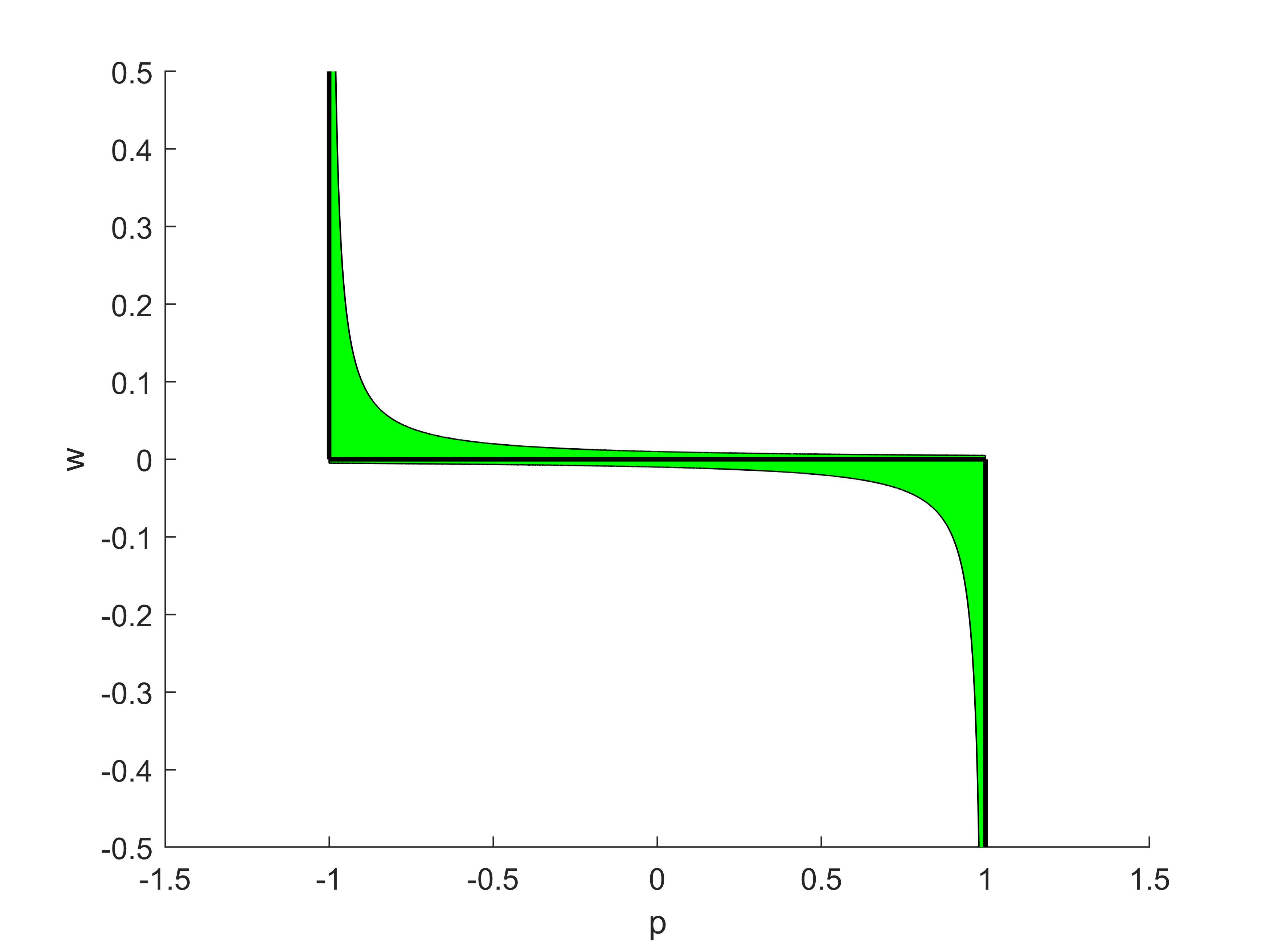
Figure 1: Relationship between BVI and its regularization reformulation. For a case with $l=-1$ and $u=1$, the black line represents BVI in the form of (7) or (8), the green region represents a strict feasible region constructed by the regularization reformulation (9) with perturbed parameter $s=0.01$

2.4 Discretized OCPEC and Optimality Conditions

For the sake of brevity, we define:

$$L(x_{n},\tau_{n},p_{n})=L_{S}(x_{n},\tau_{n},p_{n})\Delta t$$ (10a)

$$\mathcal{F}(x_{n},\tau_{n},p_{n})=f(x_{n},\tau_{n},p_{n})\Delta t-x_{n}$$ (10b)

where the terminal cost $L_{T}(x_{N},p_{N})$ is merged into the stage cost $L(x_{N},\tau_{N},p_{N})$. Subsequently, we obtain the discretized OCPEC, denoted by $\mathcal{P}_{disc}(s)$:

$$\min_{\{x_{n}\},\{\tau_{n}\},\{p_{n}\}}\sum^{N}_{n=1}L(x_{n},\tau_{n},p_{n})$$ (11)

s.t.

$$G(x_{n},\tau_{n},p_{n})\geq 0,$$ (12a)

$$C(x_{n},\tau_{n},p_{n},w_{n})=0,$$ (12b)

$$x_{n-1}+\mathcal{F}(x_{n},\tau_{n},p_{n})=0,$$ (12c)

$$\Phi(p_{n},w_{n},s)\geq 0,$$ (12d)

for all $n=1,\dots,N$, with the given initial state $x_{0}$. Here, the auxiliary variable constraints (6c) are merged into the equality constraints (12b), and the perturbed system of inequality constraints (9) forms the perturbed equilibrium constraints (12d) with $\Phi:\mathbb{R}^{n_{p}}\times\mathbb{R}^{n_{p}}\times\mathbb{R}_{+}\rightarrow\mathbb{R}^{n_{\gamma}}$. Functions $L,G,C,\mathcal{F}$ and $\Phi$ are assumed to be twice continuously differentiable. We use the shorthand for functions $F_{n}:=F(x_{n},\tau_{n},p_{n})$ in the following discussion.

$\mathcal{P}_{disc}(s)$ is a well-posed NLP problem when $s>0$. Hence, by introducing the Lagrange multiplier sequences $\{\sigma_{n}\in\mathbb{R}^{n_{\sigma}}\}$, $\{\eta_{n}\in\mathbb{R}^{n_{\eta}}\}$, $\{\lambda_{n}\in\mathbb{R}^{n_{x}}\}$ and $\{\gamma_{n}\in\mathbb{R}^{n_{\gamma}}\}$ for the inequality, equality, state equations, and perturbed equilibrium constraints, respectively, we obtain the KKT conditions associated with $\mathcal{P}_{disc}(s)$:

$$\sigma_{n}\geq 0,G_{n}\geq 0,\sigma_{n,i}G_{n,i}=0,i\in\{1,...,n_{\sigma}\},$$ (13a)

$$C_{n}=0,$$ (13b)

$$x_{n-1}+\mathcal{F}_{n}=0,$$ (13c)

$$\gamma_{n}\geq 0,\Phi_{n}\geq 0,\gamma_{n,i}\Phi_{n,i}=0,i\in\{1,...,n_{\gamma}\},$$ (13d)

$$\nabla_{x}H^{T}_{n}+\lambda_{n+1}=0,$$ (13e)

$$\nabla_{\tau}H^{T}_{n}=0,$$ (13f)

$$\nabla_{p}H^{T}_{n}=0,$$ (13g)

$$\nabla_{w}H^{T}_{n}=0,$$ (13h)

for $n=1,\dots,N$, where $\lambda_{N+1}=0$ and $x_{0}$ are provided, and $H_{n}$ denotes the Hamiltonian:

$$H_{n}:=L_{n}-\sigma^{T}_{n}G_{n}+\eta^{T}_{n}C_{n}+\lambda^{T}_{n}\mathcal{F}_{n}-\gamma^{T}_{n}\Phi_{n}.$$ (14)

Here, we merge all primal and dual variables into a vector $Y=[Y^{T}_{1},\cdots,Y^{T}_{N}]^{T}$ in a stage-wise manner with elements $Y_{n}:=[\Lambda^{T}_{n},Z^{T}_{n}]^{T}$, where $\Lambda_{n}:=[\sigma^{T}_{n},\eta^{T}_{n},\lambda^{T}_{n},\gamma^{T}_{n}]^{T}$ includes the dual variables and $Z_{n}:=[x^{T}_{n},\tau^{T}_{n},p^{T}_{n},w^{T}_{n}]^{T}$ includes the primal variables. For a given $s>0$, a point $Y(s)$ satisfying (13) is referred to as the KKT point of $\mathcal{P}_{disc}(s)$ and its primal part $Z(s)$ is referred to as the stationary point of $\mathcal{P}_{disc}(s)$. Owing to the violation of the fundamental CQs, the KKT conditions cannot be considered as the proper stationary conditions for the ill-posed NLP problem $\mathcal{P}_{disc}(0)$. However, in [16] it was proven that under certain assumptions (e.g., MPEC-MFCQ), $\lim_{s\rightarrow 0}Z(s)=Z^{*}$ and accumulation point $Z^{*}$ is a C-stationary point (a weaker stationarity notion than the KKT conditions) of $\mathcal{P}_{disc}(0)$. Moreover, the existence of sequence $\{Z(s)\}$ can be guaranteed. This constitutes the core idea of the continuation method to solve $\mathcal{P}_{disc}(0)$. Refer to [38, 37, 16] for a detailed explanation.

Remark 1.

We briefly discuss the relationship between the optimal solutions to the continuous problem $\mathcal{P}_{cont}$ and the discretized problem $\mathcal{P}_{disc}(s)$. Because DVI can be transformed into a class of differential inclusions [32], using the existing results on the optimal control of the differential inclusion [41], two conclusions can be drawn. First, the solutions of $\mathcal{P}_{disc}(0)$ converge to the solutions of $\mathcal{P}_{cont}$ as $\Delta t\rightarrow 0$; however, the gradients do not converge no matter how small we choose $\Delta t$. Second, if we choose $\Delta t=o(s)$, then the solutions and gradients of $\mathcal{P}_{disc}(s)$ converge to the solutions and gradients of $\mathcal{P}_{cont}$ as $s\rightarrow 0$. However, $\Delta t=o(s)$ is a fairly strict condition and a sufficiently small $\Delta t$ cannot be chosen practically. Hence, in this study, we consider the solution method for the ill-posed NLP problem $\mathcal{P}_{disc}(0)$ obtained by a given small enough $\Delta t$ (e.g., $0.01s$). Theoretical analysis of the approximation error is beyond the scope of this study, and we will discuss this in a future research.

3 Algorithm

In this section, a dedicated NLP solution method leveraged in the continuation method is introduced to effectively solve the ill-posed NLP problem $\mathcal{P}_{disc}(0)$.

3.1 Treatment of Inequality Constraints

In this study, we treat the inequality constraints by the smooth FB function [21]. Specifically, the complementary conditions (13a) (13d) are respectively mapped into the following perturbed systems of equations:

$$\Psi_{G,n}:=\Psi(\sigma_{n},G_{n},z)=0,$$ (15a)

$$\Psi_{\Phi,n}:=\Psi(\gamma_{n},\Phi_{n},z)=0.$$ (15b)

Here, the function $\Psi$ is defined in an element-wise manner by the smooth FB function denoted as $\psi$:

$$\psi(a,b,z)=\sqrt{a^{2}+b^{2}+z^{2}}-a-b,$$ (16)

with properties:

$$\psi(a,b,z)=0\;\Leftrightarrow\;a\geq 0,\;b\geq 0,\;ab=\frac{1}{2}z^{2},$$ (17)

where $a,b\in\mathbb{R}$, perturbed parameter $z\in\mathbb{R}_{+}$, and function $\psi$ is nonsmooth only if $z=0$. We choose the smooth FB function for two reasons: First, its favorable properties (17) indicate that it relaxes the complementarity constraint $ab=0$ in a manner similar to that adopted in IP methods (i.e., following the central path), while enforcing $a,b\geq 0$ implicitly via the function value rather than explicitly via the feasible initial guess and the fraction-to-the-boundary rule. This allows infeasible initial guess and intermediate iterates, which leads to a larger stepsize and search space against the ill-posedness of the feasible region. Second, it considers all inequality constraints at each iteration like the IP method and maps the KKT conditions into a system of equations. Hence, if this equation system is solved by the Newton method, then at each iteration the linear system has the same sparsity structure that can be exploited for faster computations through advanced linear algebra techniques. The major differences between the proposed method and [24, 25] are that, we use a $\ell_{1}$ exact penalty function as the merit function (a more reasonable choice for the constrained optimization) and design two remedy approaches against the problematic situation, which are introduced in the following.

3.2 Evaluation of Search Direction

Given $Y^{k-1},s^{k-1},z^{k-1}$, the Newton method is applied to solve the KKT conditions (13b), (13c), (13e)–(13h) and (15). This leads to the following linear equation system:

$$\mathcal{K}^{k-1}\Delta Y^{k}=-T^{k-1}.$$ (18)

Here, the KKT residual $T^{k-1}=[(T^{k-1}_{1})^{T},\cdots(T^{k-1}_{N})^{T}]^{T}$ contains elements $T^{k-1}_{n}=T(x^{k-1}_{n-1},Y^{k-1}_{n},\lambda^{k-1}_{n+1},s,z)$:

$$\begin{split}T(x_{n-1},Y_{n},\lambda_{n+1},s,z):=\begin{bmatrix}-(\nabla_{G}\Psi_{G,n})^{-1}\Psi_{G,n}\\ C_{n}\\ x_{n-1}+\mathcal{F}_{n}\\ -(\nabla_{\Phi}\Psi_{\Phi,n})^{-1}\Psi_{\Phi,n}\\ \nabla_{x}H^{T}_{n}+\lambda_{n+1}\\ \nabla_{\tau}H^{T}_{n}\\ \nabla_{p}H^{T}_{n}\\ \nabla_{w}H^{T}_{n}\end{bmatrix},\end{split}$$ (19)

and the KKT matrix $\mathcal{K}^{k-1}$ has the banded sparse structure, depicted as follows:

$$\mathcal{K}^{k-1}:=\begin{bmatrix}J^{k-1}_{1}&B_{U}&&\\ B_{L}&J^{k-1}_{2}&\ddots&\\ &\ddots&\ddots&B_{U}\\ &&B_{L}&J^{k-1}_{N}\end{bmatrix}.$$ (20)

The off-diagonal block matrices $B_{L}$ and $B_{U}$ are sparse and formed by the identity matrix $I_{n_{x}}\in\mathbb{R}^{n_{x}\times n_{x}}$ and the zero matrix $0$ with appropriate dimension:

$$B_{L}=\begin{bmatrix}0&0&0&0\\ 0&0&0&B_{I}\\ 0&0&0&0\\ 0&0&0&0\end{bmatrix},\quad B_{U}=B^{T}_{L},\quad B_{I}=\begin{bmatrix}0&0\\ I_{n_{x}}&0\end{bmatrix},$$ (21)

while the main diagonal block matrix $J^{k-1}_{n}$ is symmetric:

$$\begin{split}&J_{n}=J(Y_{n},s,z)\\ &:=\begin{bmatrix}D_{n}&0&0&-\nabla_{Z}G_{n}\\ 0&-\nu_{J}I&0&\nabla_{Z}A_{n}\\ 0&0&E_{n}&-\nabla_{Z}\Phi_{n}\\ -\nabla_{Z}G^{T}_{n}&\nabla_{Z}A^{T}_{n}&-\nabla_{Z}\Phi^{T}_{n}&\nabla_{ZZ}H_{n}\end{bmatrix}\\ \end{split},$$ (22)

where:

$$\nabla_{Z}A_{n}=\begin{bmatrix}\nabla_{Z}C_{n}\\ \nabla_{Z}\mathcal{F}_{n}\\ \end{bmatrix},\quad D_{n}=\text{diag}(d_{n}),\quad E_{n}=\text{diag}(e_{n}),$$ (23)

with the vectors $d_{n}\in\mathbb{R}^{n_{\sigma}},e_{n}\in\mathbb{R}^{n_{\gamma}}$:

$$d_{n,i}=-\frac{\sigma_{n,i}-\sqrt{(G_{n,i})^{2}+(\sigma_{n,i})^{2}+z^{2}}-\nu_{G}}{G_{n,i}-\sqrt{(G_{n,i})^{2}+(\sigma_{n,i})^{2}+z^{2}}-\nu_{G}},$$ (24a)

$$e_{n,i}=-\frac{\gamma_{n,i}-\sqrt{(\Phi_{n,i})^{2}+(\gamma_{n,i})^{2}+z^{2}}-\nu_{G}}{\Phi_{n,i}-\sqrt{(\Phi_{n,i})^{2}+(\gamma_{n,i})^{2}+z^{2}}-\nu_{G}}.$$ (24b)

Two regularization parameters $\nu_{J},\nu_{G}\in\mathbb{R}_{+}$ are introduced (in our setting $\nu_{J},\nu_{G}=10^{-7}$) to avoid the singularity caused by the rank-deficiency of $\nabla_{Z}A_{n}$ and the non-negative definiteness of $D_{n},E_{n}$ (see Lemma 1 in Section 4). Here, we enforce $D_{n},E_{n}<0$ to mitigate the previously mentioned numerical difficulties caused by the near linear dependence of active inequalities defined in (12d). Specifically, if $z=0$, then $\nu_{G}>0$ can guarantee the negative definiteness of $D_{n}$ and $E_{n}$; if $z>0$, then $D_{n}$ and $E_{n}$ are inherently negative definite even though setting $\nu_{G}=0$. We find that setting a small value to $\nu_{G}$ is sufficiently effective in our numerical experience, and an improvement in numerical performance can be expected if designing sophisticated rules that adaptively adjust $\nu_{G}$ to handle the ill-conditioned KKT matrix $\mathcal{K}$.

The special sparse structure of $\mathcal{K}^{k-1}$ facilitates an efficient solution method for the linear system (18) by exploiting the sparsity with a Riccati-like recursion. Namely, we can first transform $\mathcal{K}^{k-1}$ into a lower triangular matrix by performing a backward recursion from $n=N$ to $1$ using:

$$\begin{split}&\mathfrak{A}^{k-1}_{N}=J^{k-1}_{N},\qquad\mathfrak{b}^{k-1}_{N}=T^{k-1}_{N},\\ &\mathfrak{A}^{k-1}_{n}=J^{k-1}_{n}-B_{U}(\mathfrak{A}^{k-1}_{n+1})^{-1}B_{L},\\ &\mathfrak{b}^{k-1}_{n}=T^{k-1}_{n}-B_{U}(\mathfrak{A}^{k-1}_{n+1})^{-1}\mathfrak{b}^{k-1}_{n+1}.\end{split}$$ (25)

Then we can evaluate the search direction by performing a forward recursion from $n=1$ to $N$ using:

$$\begin{split}&\Delta Y^{k}_{0}=0,\\ &\Delta Y^{k}_{n}=-(\mathfrak{A}^{k-1}_{n})^{-1}(\mathfrak{b}^{k-1}_{n}+B_{L}\Delta Y^{k}_{n-1}).\end{split}$$ (26)

3.3 Merit Line Search

After evaluating the full-step search direction $\Delta Y^{k}$, in order to guarantee the convergence from a poor initial guess, we evaluate the stepsize $\alpha$ by the merit line search procedure inspired by [46, 28], with a merit function $\Theta(Y)$ defined by the following $\ell_{1}$ exact penalty function:

$$\Theta(Y)=\sum^{N}_{n=1}L_{n}+\beta\sum^{N}_{n=1}M_{n},$$ (27)

where $M_{n}$ denotes the constraint violation:

$$\begin{split}&M_{n}:=M(\sigma_{n},\gamma_{n},Z_{n})\\ &=\|\Psi_{G,n}\|_{1}+\|C_{n}\|_{1}+\|x_{n-1}+\mathcal{F}_{n}\|_{1}+\|\Psi_{\Phi,n}\|_{1},\end{split}$$ (28)

and $\beta$ is the penalty parameter that satisfies

$$\beta\geq\beta_{trail}:=\frac{\sum^{N}_{n=1}\nabla_{Z}L^{k-1}_{n}\Delta Z^{k}_{n}}{(1-\rho)\sum^{N}_{n=1}M^{k-1}_{n}},$$ (29)

with $\rho=0.1$. Let $\mathbb{D}\Theta^{k-1,k}$ denote the directional derivative of the merit function (27) at the current iterate $Y^{k-1}$ along the given direction $\Delta Y^{k}$. Owing to the properties of $\ell_{1}$ function [28], we have:

$$\begin{split}\mathbb{D}\Theta^{k-1,k}:=\sum^{N}_{n=1}\nabla_{Z}L^{k-1}_{n}\Delta Z^{k}_{n}-\beta\sum^{N}_{n=1}M^{k-1}_{n}.\end{split}$$ (30)

The choice of the penalty parameter (29) is based on the fact that $\mathbb{D}\Theta^{k-1,k}$ is forced to be sufficiently negative in the sense that:

$$\begin{split}\mathbb{D}\Theta^{k-1,k}\leq-\rho\beta\sum^{N}_{n=1}M^{k-1}_{n}.\end{split}$$ (31)

We perform a backtracking line search strategy by gradually reducing the trail stepsize $\alpha_{trail}\leftarrow\nu_{\alpha}\alpha_{trail}$ from $\alpha_{max}$ to $\alpha_{min}$ until the Armijo condition is satisfied:

$$\Theta(Y^{k-1}+\alpha_{trail}\Delta Y^{k})\leq\Theta(Y^{k-1})+\nu_{D}\alpha_{trail}\mathbb{D}\Theta^{k-1,k}.$$ (32)

In the proposed method, emphasize again, we can set $\alpha_{max}=1$ without the fraction-to-the-boundary rules to enforce the primal and dual feasibility. In our setting $\alpha_{min}=0.01$, $\nu_{\alpha}=0.7$ and $\nu_{D}=10^{-4}$.

3.4 Second Order Correction

Some steps that achieve good progress toward the solution may be rejected by the merit function, which is a phenomenon known as the Maratos effect. Some off-the-shelf NLP solvers overcome this deficiency by applying the second order corrections (SOC) to improve feasibility [28]. Briefly, SOC corrects the full-step direction $\Delta Y^{k}$ with an additional Newton-type step $\Delta Y^{k}_{soc}$ called the SOC step, using the constraint Jacobian evaluated at the current iterate $Y^{k-1}$ and the constraint function evaluated at the full-step iterate $Y^{k}_{fs}=Y^{k-1}+\Delta Y^{k}$. In the proposed method, a dedicated SOC is employed if the first trial stepsize $\alpha_{trail}=1$ is rejected only because of the increase in constraint violation, namely, $\alpha_{trail}=1$ fails to satisfy (32) but reduces the total cost:

$$\sum^{N}_{n=1}L(Y^{k}_{fs,n})\leq\sum^{N}_{n=1}L(Y^{k-1}_{n}).$$ (33)

Then, before reducing the trail stepsize, we attempt a corrected search direction $\Delta Y^{k}_{cor}=\Delta Y^{k}+\Delta Y^{k}_{soc}$ by solving a linear equation system extended from (18):

$$\mathcal{K}^{k-1}\Delta Y^{k}_{cor}=-(T^{k-1}+T^{k}_{cor}),$$ (34)

where $T^{k}_{cor}=[(T^{k}_{cor,1})^{T},\cdots(T^{k}_{cor,N})^{T}]^{T}$ is a correction term with $T^{k}_{cor,n}$ formed by the Jacobian of smooth FB function evaluated at the current iterate $Y^{k-1}$ and constraint function evaluated at the full-step iterate $Y^{k}_{fs}$:

$$T^{k}_{cor,n}:=\begin{bmatrix}-(\nabla_{G}\Psi^{k-1}_{G,n})^{-1}\Psi(\sigma^{k}_{fs,n},G^{k}_{fs,n},z)\\ C^{k}_{fs,n}\\ x^{k}_{fs,n-1}+\mathcal{F}^{k}_{fs,n}\\ -(\nabla_{\Phi}\Psi^{k-1}_{\Phi,n})^{-1}\Psi(\gamma^{k}_{fs,n},\Phi^{k}_{fs,n},z)\\ 0_{(n_{\tau}+n_{x}+n_{p}+n_{w})\times 1}\end{bmatrix}.$$ (35)

Once the corrected search direction $\Delta Y^{k}_{cor}$ has been computed, we define a SOC trail iterate $Y^{k}_{soc}=Y^{k-1}+\Delta Y^{k}_{cor}$ and accept it as a new iterate if it satisfies:

$$\Theta(Y^{k}_{soc})\leq\Theta(Y^{k-1}).$$ (36)

Otherwise, we discard this corrected direction $\Delta Y^{k}_{cor}$ and resume the regular backtracking line search with a smaller trail stepsize $\alpha_{trail}$ along the original direction $\Delta Y^{k}$. Note that because constraints at the full-step iterate $Y^{k}_{fs}$ have been evaluated when testing the acceptance of $\alpha_{trail}=1$, the right-hand side of system (34) does not require any additional constraint evaluation but only some simple basic operations, such as left multiplication by the inverse of the diagonal matrix in the first and fourth block of (35). On the left-hand side of system (34), the matrix $\mathcal{K}^{k-1}$ is identical to that in system (18); hence, we can solve system (34) using the same sparsity exploitation method as we applied in (18). In summary, the computation cost of a SOC step is one forward and one backward recursion for solving the linear equation system, and one additional evaluation of the merit function to test the acceptance of $Y^{k}_{soc}$ in (36).

3.5 Feasibility Restoration Phase

Some off-the-shelf NLP solvers, e.g., IPOPT [45], have a remedy mode called the feasibility restoration phase (FRP) to improve solver robustness when struggling with finding a solution owing to certain problematic circumstances. For example, the backtracking line search strategy may stall or fail to find a proper new iterate if the acceptable stepsize is arbitrarily small. Moreover, FRP is often invoked as an infeasibility detection to inform the user of problematic situations and terminate the inefficient iteration in time. Considering that the NLP problem $\mathcal{P}_{disc}(s)$ we solve is essentially an ill-posed NLP problem, numerical difficulties occur frequently even though $\mathcal{P}_{disc}(s)$ is relieved to some extent by $s$. Hence, a dedicated FRP is employed as a remedy mode whenever the regular progress to solution encounters numerical difficulties that cause it to struggle in continuing with the regular iterations.

Briefly, FRP aims to provide the regular progress to solution with a new iterate $Y^{k}_{frp}$, which not only decreases the constraint violation but also attempts to avoid a large deviation from the iterate $Y^{k-1}$ that switches to FRP (referred to as the start iterate in the following). In the proposed method, FRP achieves this goal by solving the following NLP problem:

$$\min_{\bar{Z}}\sum^{N}_{n=1}\frac{1}{2}(\bar{Z}_{n}-\bar{Z}^{R}_{n})^{T}D_{sc,n}(\bar{Z}_{n}-\bar{Z}^{R}_{n})$$ (37)

s.t.

$$G(\bar{x}_{n},\bar{\tau}_{n},\bar{p}_{n})\geq 0,$$ (38a)

$$C(\bar{x}_{n},\bar{\tau}_{n},\bar{p}_{n},\bar{w}_{n})=0,$$ (38b)

$$\bar{x}_{n-1}+\mathcal{F}(\bar{x}_{n},\bar{\tau}_{n},\bar{p}_{n})=0,$$ (38c)

$$\Phi(\bar{w}_{n},\bar{p}_{n},s)\geq 0,$$ (38d)

for all $n=1,\dots,N$. In order to avoid confusion, in FRP, we use overbars $\bar{Y}$ to denote variables and superscript $j$ for the iteration counter. This NLP problem (37) (38) has primal variables $\bar{Z}=[\bar{Z}^{T}_{1},\cdots\bar{Z}^{T}_{N}]^{T}$ with elements $\bar{Z}_{n}=[\bar{x}^{T}_{n},\bar{\tau}^{T}_{n},\bar{p}^{T}_{n},\bar{w}^{T}_{n}]^{T}\in\mathbb{R}^{n_{Z}}$. We choose the reference point to be the start iterate $\bar{Z}^{R}_{n}=Z^{k-1}_{n}$, and define a scaling matrix $D_{sc,n}=\nu_{sc}\text{diag}(d_{sc,n})\in\mathbb{R}^{n_{Z}\times n_{Z}}$ with a scaling parameter $\nu_{sc}=10^{-6}$ and a vector $d_{sc,n}\in\mathbb{R}^{n_{Z}}$ whose elements are:

$$d_{sc,n,i}=\min\{1,1/|\bar{Z}^{R}_{n,i}|\}.$$ (39)

Hence, this NLP problem (37) (38) is of the form (11) (12) and can be solved by the proposed non-interior-point NLP solution method. Note that in FRP, we neither apply SOC nor update the perturbed parameter during the iterations (i.e., $\bar{s}^{0}\equiv\bar{s}^{j}\equiv s^{k-1}$, $\bar{z}^{0}\equiv\bar{z}^{j}\equiv z^{k-1}$). To solve this NLP problem, we respectively initialize primal variables and dual variables of the inequality constraints using the start iterate, that is, $\bar{Z}^{0}=Z^{k-1}$, $\bar{\sigma}^{0}=\sigma^{k-1}$ and $\bar{\gamma}^{0}=\gamma^{k-1}$, and initialize dual variables of the equality constraints by $\bar{\eta}^{0},\bar{\lambda}^{0}=0$. Here, we do not exactly solve this NLP problem (37) (38), instead, the iteration is terminated if the constraint violation of the current iterate ($\bar{\sigma}^{j}$, $\bar{\gamma}^{j}$, $\bar{Z}^{j}$) has been decreased to a desired level compared with that of the start iterate $(\sigma^{k-1},\gamma^{k-1},Z^{k-1})$:

$$\sum^{N}_{n=1}M(\bar{\sigma}^{j}_{n},\bar{\gamma}^{j}_{n},\bar{Z}^{j}_{n})\leq\nu_{M}\sum^{N}_{n=1}M(\sigma^{k-1}_{n},\gamma^{k-1}_{n},Z^{k-1}_{n})$$ (40)

where $\nu_{M}=0.9$ is the scaling parameter. Then we respectively set primal variables and dual variables of the inequality constraints in $Y^{k}_{frp}$ by $Z^{k}_{frp}=\bar{Z}^{j}$, $\sigma^{k}_{frp}=\bar{\sigma}^{j}$ and $\gamma^{k}_{frp}=\bar{\gamma}^{j}$. For the dual variables of the equality constraints $\eta^{k}_{frp}$ and $\lambda^{k}_{frp}$, these quantities can be obtained as the minimum norm least-square solution for the dual feasibility (13e)–(13h) based on the calculated $Z^{k}_{frp}$, $\sigma^{k}_{frp}$ and $\gamma^{k}_{frp}$, that is, by solving the overdetermined linear equation system:

$$\begin{split}\begin{bmatrix}(\nabla_{Z}C^{k}_{frp,n})^{T}&(\nabla_{Z}\mathcal{F}^{k}_{frp,n})^{T}\end{bmatrix}\begin{bmatrix}\eta^{k}_{frp,n}\\ \lambda^{k}_{frp,n}\end{bmatrix}=-\mathfrak{B}^{k}_{frp,n}\end{split}$$ (41)

where:

$$\begin{split}\mathfrak{B}^{k}_{frp,n}&=(\nabla_{Z}L^{k}_{frp,n})^{T}-(\nabla_{Z}G^{k}_{frp,n})^{T}\sigma^{k}_{frp,n}\\ &-(\nabla_{Z}\Phi^{k}_{frp,n})^{T}\gamma^{k}_{frp,n}+\begin{bmatrix}\lambda^{k}_{frp,n+1}\\ 0_{(n_{\tau}+n_{p}+n_{w})\times 1}\end{bmatrix}.\end{split}$$ (42)

This overdetermined system can be solved by the complete orthogonal decomposition (COD) in a backward recursion manner from $n=N$ to 1 with $\lambda^{k}_{frp,N+1}=0$. If results are too large, that is, $\|[(\eta^{k}_{frp})^{T},(\lambda^{k}_{frp})^{T}]^{T}\|_{\infty}\geq\Lambda_{max}$ (in our setting $\Lambda_{max}=1000$), then we reset these quantities by $\eta^{k}_{frp},\lambda^{k}_{frp}=0$.

Remark 2 (Infeasibility detection).

Sometimes the FRP also encounters certain problematic situations. For example, it may fail to find a appropriate iterate satisfying (40) within the maximum iteration number $j_{max}$ (in our setting $j_{max}=20$), or the backtracking line search in FRP may fail again owing to the small stepsize. At this time the FRP will return an error message and terminate the overall routine because such problematic circumstances indicate the difficulty in finding a more feasible iterate near the current iterate. Accordingly, the inefficient iteration should be terminated in time.

3.6 Summaries of the Algorithm

Algorithm 1 Non-Interior-Point NLP Solution Method

Inputs: $Y^{0},s^{0},z^{0}$

Outputs: $Y^{*}$

Initialization: $Y^{k-1}\leftarrow Y^{0},s^{k-1}\leftarrow s^{0},z^{k-1}\leftarrow z^{0}$

Initialization: findOptimalSolution $\leftarrow$ false

for $k=1\text{ to }k_{max}$ do

     Step 1: check termination condition

     if (43) and one of the (44) are satisfied then

         findOptimalSolution $\leftarrow$ true

     end if

     Step 2: return optimal solution

     if findOptimalSolution = true then

         $Y^{*}\leftarrow Y^{k-1}$

         break

     end if

     Step 3: evaluation of search direction

     $(\Delta Y^{k},T^{k-1},\mathcal{K}^{k-1})\leftarrow\newline \hskip 30.00005pt\text{SEARCHDIRECTION}(Y^{k-1},s^{k-1},z^{k-1})$

     Step 4: merit line search with SOC

     $(Y^{k},\text{flag})\leftarrow\text{MLSSOC}(Y^{k-1},s^{k-1},z^{k-1},\newline \hskip 30.00005pt\Delta Y^{k},T^{k-1},\mathcal{K}^{k-1})$

     if flag = failure then

         $Y^{k}_{frp}\leftarrow\text{FRP}(Y^{k-1},s^{k-1},z^{k-1})$

         $Y^{k}\leftarrow Y^{k}_{frp}$

     end if

     Step 5: update perturbed parameters

     if (45) is satisfied then

         $(s^{k},z^{k})\leftarrow\text{using }(\ref{updatesz_rules})\text{ with }s^{k-1},z^{k-1}$

     else

         $s^{k}\leftarrow s^{k-1},z^{k}\leftarrow z^{k-1}$

     end if

end for

Algorithm 2 Newton Step

function NewtonStep($T^{k-1},\mathcal{K}^{k-1}$)

     Step 1: backward recursion

     for $n=N\text{ to }1$ do

         $(\mathfrak{A}^{k-1}_{n},\mathfrak{b}^{k-1}_{n})\leftarrow(T^{k-1},\mathcal{K}^{k-1})$ $\triangleright$ (25)

     end for

     Step 2: forward recursion

     for $n=1\text{ to }N$ do

         $\Delta Y^{k}_{n}\leftarrow(\mathfrak{A}^{k-1}_{n},\mathfrak{b}^{k-1}_{n})$ $\triangleright$ (26)

     end for

     return $\Delta Y^{k}$

end function

Algorithm 3 Evaluation of Search Direction

$\textbf{Inputs}:\nu_{J}$

function searchdirection($Y^{k-1},s^{k-1},z^{k-1}$)

     Step 1: evaluate KKT residual and matrix

     $T^{k-1}\leftarrow(Y^{k-1},s^{k-1},z^{k-1})$ $\triangleright$ (19)

     $\mathcal{K}^{k-1}\leftarrow(Y^{k-1},s^{k-1},z^{k-1},\nu_{J})$ $\triangleright$ (20)

     Step 2: Newton Step

     $\Delta Y^{k}\leftarrow\text{NEWTONSTEP}(T^{k-1},\mathcal{K}^{k-1})$

     return $\Delta Y^{k},T^{k-1},\mathcal{K}^{k-1}$

end function

Our algorithm follows the procedures of the continuation method. At the beginning of each iteration, we check the given $Y^{k-1},s^{k-1},z^{k-1}$ and return $Y^{k-1}$ as the optimal solution $Y^{*}$ if $s^{k-1}$ and $z^{k-1}$ have been decreased to sufficiently small desired value $s^{*},z^{*}$:

$$s^{k-1}\leq s^{*},z^{k-1}\leq z^{*}$$ (43)

and one of the following termination conditions associated with infeasibility is satisfied:

$$\|T^{k-1}_{p}\|_{\infty}\leq\mathfrak{T}_{p}$$ (44a)

$$\|T^{k-1}_{d}\|_{\infty}\leq\mathfrak{T}_{d}$$ (44b)

$$\text{max}\{\|T^{k-1}_{p}\|_{\infty},\|T^{k-1}_{d}\|_{\infty}\}\leq\mathfrak{T}_{max}$$ (44c)

where $T^{k-1}_{p}=[(T^{k-1}_{p,1})^{T},\cdots(T^{k-1}_{p,N})^{T}]^{T}$ denotes the primal infeasibility with elements $T^{k-1}_{p,n}$ formulated by (13b), (13c), (15), and $T^{k-1}_{d}=[(T^{k-1}_{d,1})^{T},\cdots(T^{k-1}_{d,N})^{T}]^{T}$ denotes the dual infeasibility with elements $T^{k}_{d,n}$ formulated by scaling (13e)–(13h) with the dual variables [45]. Here, $\mathfrak{T}_{p},\mathfrak{T}_{d},\mathfrak{T}_{max}$ are the desired tolerances.

At the end of each iteration, we check the primal infeasibility and if it satisfies:

$$\|T^{k}_{p}\|_{\infty}\leq 10\mathfrak{T}_{p}$$ (45a)

then, inspired by the update rules for the barrier parameter stated in [45], we decrease the perturbed parameters $s,z$ based on the following:

$$s^{k}=\max\{\min\{\kappa_{st}s^{k-1},(s^{k-1})^{\kappa_{se}}\},s^{*}\}$$ (46a)

$$z^{k}=\max\{\min\{\kappa_{zt}z^{k-1},(z^{k-1})^{\kappa_{ze}}\},z^{*}\}$$ (46b)

where $\kappa_{st},\kappa_{zt}=0.2,\kappa_{se},\kappa_{ze}=1.5$ in our setting. Otherwise, we maintain $s^{k}=s^{k-1},z^{k}=z^{k-1}$ for the next iteration.

Algorithm 1 summarizes the proposed non-interior-point method. Algorithms 2 and 3 summarize the evaluation of search direction as discussed in Section 3.2. Algorithm 4 summarizes the merit line search procedure with the second order correction as discussed in Section 3.3 and 3.4. Algorithm 5 summarizes the feasibility restoration phase as discussed in Section 3.5.

Algorithm 4 Merit Line Search with Second Order Correction

Inputs: $\nu_{\alpha},\nu_{D},\alpha_{min}$

function mlssoc($Y^{k-1},s^{k-1},z^{k-1},\Delta Y^{k},T^{k-1},\newline \hskip 60.00009pt\mathcal{K}^{k-1}$)

     Initialization: $\alpha_{trail}\leftarrow 1$

     Initialization: NewIterate $\leftarrow$ false

     while NewIterate = false do

         if $\alpha_{trail}\text{ satisfies Armijo condition (\ref{ArmijoCondition})}$ then

              $Y^{k}\leftarrow Y^{k-1}+\alpha_{trail}\Delta Y^{k}$

              NewIterate $\leftarrow$ true

              flag $\leftarrow$ success

         else if $\alpha_{trail}=1\text{ and satisfies (\ref{SOC_startCondition})}$ then

              $Y^{k}_{fs}\leftarrow Y^{k}$

              $T^{k}_{cor}\leftarrow(Y^{k-1},Y^{k}_{fs})$ $\triangleright$ (35)

              $T^{k-1}\leftarrow T^{k-1}+T^{k}_{cor}$

              $\Delta Y^{k}_{cor}\leftarrow\text{NEWTONSTEP}(T^{k-1},\mathcal{K}^{k-1})$

              $Y^{k}_{soc}\leftarrow Y^{k-1}+\Delta Y^{k}_{cor}$

              if  $Y^{k}_{soc}\text{ satisfies (\ref{SOC_test})}$ then

                  $Y^{k}\leftarrow Y^{k}_{soc}$

                  NewIterate $\leftarrow$ true

                  flag $\leftarrow$ success

              else

                  $\alpha_{trail}=\text{max}(\nu_{\alpha}\alpha_{trail},\alpha_{min})$

              end if

         else

              $\alpha_{trail}=\text{max}(\nu_{\alpha}\alpha_{trail},\alpha_{min})$

         end if

         if $\alpha_{trail}=\alpha_{min}$ and NewIterate = false then

              $Y^{k}\leftarrow Y^{k-1}$

              flag $\leftarrow$ failure

              break

         end if

     end while

     return $Y^{k},\text{flag}$

end function

Algorithm 5 Feasibility Restoration Phase

Inputs: $\nu_{sc},\nu_{M},\Lambda_{max},j_{max}$

function FRP($Y^{k-1},s^{k-1},z^{k-1}$)

     Initialization: $\bar{Z}^{j-1},\bar{\sigma}^{j-1},\bar{\gamma}^{j-1}\leftarrow Y^{k-1}$

     Initialization: $\bar{\eta}^{j-1},\bar{\lambda}^{j-1}\leftarrow 0$

     Initialization: $\bar{s}^{j-1}\equiv s^{k-1},\bar{z}^{j-1}\equiv z^{k-1}$

     Initialization: findFeasibleSolution $\leftarrow$ false

     $\bar{Y}^{j-1}\leftarrow(\bar{\sigma}^{j-1},\bar{\eta}^{j-1},\bar{\lambda}^{j-1},\bar{\gamma}^{j-1},\bar{Z}^{j-1})$

     for $j=1\text{ to }j_{max}$ do

         Step 1: check termination condition

         if (40) is satisfied then

              findFeasibleSolution $\leftarrow$ true

         end if

         Step 2: return feasible solution

         if findFeasibleSolution = true then

              $Z^{k}_{frp},\sigma^{k}_{frp},\gamma^{k}_{frp}\leftarrow\bar{Y}^{j-1}$

              $\eta^{k}_{frp},\lambda^{k}_{frp}\leftarrow(Z^{k}_{frp},\sigma^{k}_{frp},\gamma^{k}_{frp})$ $\triangleright$ (41)

              $Y^{k}_{frp}\leftarrow(\sigma^{k}_{frp},\eta^{k}_{frp},\lambda^{k}_{frp},\gamma^{k}_{frp},Z^{k}_{frp})$

              break

         end if

         Step 3: evaluation of search direction

         $(\Delta\bar{Y}^{j},\bar{T}^{j-1},\bar{\mathcal{K}}^{j-1})\leftarrow\newline \hskip 50.00008pt\text{SEARCHDIRECTION}(\bar{Y}^{j-1},\bar{s}^{j-1},\bar{z}^{j-1})$

         Step 4: merit line search without SOC

         $(\bar{Y}^{j},\text{flag})\leftarrow\text{MLSSOC}(\bar{Y}^{j-1},\bar{s}^{j-1},\bar{z}^{j-1},\newline \hskip 50.00008pt\Delta\bar{Y}^{j},\bar{T}^{j-1},\bar{\mathcal{K}}^{j-1})$ $\triangleright$ turn off SOC

         if flag = failure then

              $Y^{k}_{frp}\leftarrow Y^{k-1}$

              break

         end if

     end for

     return $Y^{k}_{frp}$

end function

4 Convergence Analysis

4.1 Local Convergence

In this subsection, we investigate the local convergence behaviour of the iterate sequence generated by the proposed method with the perturbed parameters $s^{*},z^{*}>0$.

Assumption 1.

For any given $s,z>0$, in (22) the Hessian matrix $\nabla_{ZZ}H_{n}$ is semi-positive definite, and the Jacobian of the equality-type constraints $\nabla_{Z}A_{n}$ has full row rank.

Based on Assumption 1 and the given $z>0$, we can set the regularization parameters $\nu_{J},\nu_{G}=0$. In the following, we first demonstrate the nonsingularity of the KKT matrix $\mathcal{K}$ and its main diagonal block matrix $J(Y_{n},s,z)$ using the following lemmas.

Lemma 1.

Let Assumption 1 hold and pick $s,z>0$. Then, $J(Y_{n},s,z)$ is nonsingular for any $Y_{n}\in\mathbb{R}^{n_{Y}}$

Suppose that $J_{n}$ is singular, then, there exists a non-zero vector $q\in\mathbb{R}^{n_{Y}}$ such that $J_{n}q=0$. By dividing $q=[q^{T}_{1},q^{T}_{2},q^{T}_{3},q^{T}_{4}]$ with $q_{1}\in\mathbb{R}^{n_{\sigma}}$, $q_{2}\in\mathbb{R}^{n_{\eta}+n_{\lambda}}$, $q_{3}\in\mathbb{R}^{n_{\gamma}}$ and $q_{4}\in\mathbb{R}^{n_{Z}}$, we have:

$$\begin{split}&D_{n}q_{1}-\nabla_{Z}G_{n}q_{4}=0,\\ &\nabla_{Z}A_{n}q_{4}=0,\\ &E_{n}q_{3}-\nabla_{Z}\Phi_{n}q_{4}=0,\\ &\nabla_{ZZ}H_{n}q_{4}-\nabla_{Z}G^{T}_{n}q_{1}+\nabla_{Z}A^{T}_{n}q_{2}-\nabla_{Z}\Phi^{T}_{n}q_{3}=0.\end{split}$$ (47)

Considering that the diagonal matrices $D_{n}$ and $E_{n}$ are inherently negative definite for given $z>0$, substituting the first and third equations into the fourth equation in (47), we have:

$$R_{n}q_{4}=\nabla_{Z}A^{T}_{n}q_{2},$$ (48)

with

$$R_{n}=\nabla_{ZZ}H_{n}-\nabla_{Z}G^{T}_{n}D^{-1}_{n}\nabla_{Z}G_{n}-\nabla_{Z}\Phi^{T}_{n}E^{-1}_{n}\nabla_{Z}\Phi_{n}.$$ (49)

Owing to $D_{n},E_{n}<0$ and $\nabla_{ZZ}H_{n}\geq 0$, one can demonstrate that $R_{n}$ is positive definite and invertible. Hence, by substituting (48) into the second equation in (47), we have:

$$(\nabla_{Z}A_{n}R_{n}^{-1}\nabla_{Z}A^{T}_{n})q_{2}=0.$$ (50)

Because matrix $\nabla_{Z}A_{n}$ has full row rank, one can demonstrate that $\nabla_{Z}A_{n}R_{n}^{-1}\nabla_{Z}A^{T}_{n}$ is positive definite, accordingly, we have $q_{2}=0$. Consequently, $q_{1},q_{3},q_{4}=0$, and we have the vector $q=0$, which contradicts the assumption at the beginning that $q$ is a non-zero vector. This completes the proof. ∎

Lemma 2.

Let Assumption 1 hold and pick $s,z>0$. Subsequently, the KKT matrix $\mathcal{K}$ is nonsingular.

We provide a proof by checking the Riccati-like recursion (25) (26). From Lemma 1, we can guarantee the nonsingularity of $\mathfrak{A}_{N}=J_{N}$. Next, we check the nonsingularity of $\mathfrak{A}_{N-1}=J_{N-1}-B_{U}\mathfrak{A}^{-1}_{N}B_{L}$. Suppose that $J^{-1}_{N}$ has the following form:

$$J^{-1}_{N}=\begin{bmatrix}\hat{J}_{1,1,N}&\hat{J}_{1,2,N}&\hat{J}_{1,3,N}&\hat{J}_{1,4,N}\\ \hat{J}_{2,1,N}&\hat{J}_{2,2,N}&\hat{J}_{2,3,N}&\hat{J}_{2,4,N}\\ \hat{J}_{3,1,N}&\hat{J}_{3,2,N}&\hat{J}_{3,3,N}&\hat{J}_{3,4,N}\\ \hat{J}_{4,1,N}&\hat{J}_{4,2,N}&\hat{J}_{4,3,N}&\hat{J}_{4,4,N}\end{bmatrix}$$ (51)

with appropriate block matrix dimensions. From (25), we must compute $B_{U}J^{-1}_{N}B_{L}$. By performing some block matrix calculations, we have:

$$B_{U}J^{-1}_{N}B_{L}=\begin{bmatrix}0&0&0&0\\ 0&0&0&0\\ 0&0&0&0\\ 0&0&0&B^{T}_{I}\hat{J}_{2,2,N}B_{I}\\ \end{bmatrix}.$$ (52)

Based on $J^{-1}_{N}J_{N}=I$ and the block matrix structures defined by (51) and (22), we have:

$$\hat{J}_{2,2,N}=-(\nabla_{Z}A_{N}R_{N}^{-1}\nabla_{Z}A^{T}_{N})^{-1},$$ (53)

where the matrix $R_{N}$ is defined by (49). Hence $\hat{J}_{2,2,N}$ is negative definite and $B^{T}_{I}\hat{J}_{2,2,N}B_{I}<0$. Consequently, $\mathfrak{A}_{N-1}=J_{N-1}-B_{U}\mathfrak{A}^{-1}_{N}B_{L}$ has the same block matrix structure as $J_{N-1}$ and does not violate Assumption 1, which guarantee its nonsingularity. Recursively, we can guarantee the nonsingularity of $\mathfrak{A}_{n}$ for $n=1,\cdots,N$. Hence, from the Riccati-like recursion (25) (26) we can write down $\Delta Y=\mathcal{K}^{-1}T$. This completes the proof. ∎

Because $\mathcal{P}_{disc}(s)$ is a well-posed NLP problem when $s>0$, the existence of iterate sequence $\{Y^{k}\}$ can be guaranteed. Subsequently, there exists an index $\hat{k}$ such that for $k-1\geq\hat{k}$, we have $s^{k-1}=s^{k}=...=s^{*}$ and $z^{k-1}=z^{k}=...=z^{*}$. Hence, we only demonstrate that the proposed method has a quadratic local convergence rate for fixed $s^{*},z^{*}>0$. We make an assumption regarding the property of KKT matrix $\mathcal{K}$ for the proof of the local convergence rate.

Assumption 2.

For any given $s,z>0$, $\mathcal{K}$ is a locally Lipschitz continuous function, namely, for every $Y\in\mathbb{R}^{Nn_{Y}}$, there exists a Lipschitz constant $\xi_{L}(Y)>0$ and a neighborhood $\mathcal{Y}_{L}(Y)$ of $Y$ such that:

$$\|\mathcal{K}(Y+\Delta Y)-\mathcal{K}(Y)\|\leq\xi_{L}\|\Delta Y\|,\forall(Y+\Delta Y)\in\mathcal{Y}_{L}(Y).$$ (54)

Theorem 1.

For any fixed $s^{*},z^{*}>0$, let Assumptions 1 and 2 hold, and $Y^{*}$ be the solution of $T^{*}:=T(Y,s^{*},z^{*})=0$. Then, there exists a neighborhood $\mathcal{Y}_{C}(Y^{*})$ of $Y^{*}$ such that for every $Y^{0}\in\mathcal{Y}_{C}(Y^{*})$, the iterate sequence $\{Y^{k}\}$ generated by the proposed method remains in $\mathcal{Y}_{C}(Y^{*})$ and converges to $Y^{*}$ quadratically.

We have the distance between $Y^{k}$ and $Y^{*}$:

$$\begin{split}&\|Y^{k}-Y^{*}\|\\ =&\|Y^{k-1}+\Delta Y^{k}-Y^{*}\|\\ =&\|Y^{k-1}-(\mathcal{K}^{k-1})^{-1}T^{k-1}-Y^{*}\|\\ \leq&\|(\mathcal{K}^{k-1})^{-1}\|\|\mathcal{K}^{k-1}(Y^{k-1}-Y^{*})-(T^{k-1}-T^{*})\|.\end{split}$$ (55)

For the first term $\|(\mathcal{K}^{k-1})^{-1}\|$, Lemma 2 states that there exist a neighborhood $\mathcal{Y}_{\mathcal{K}}(Y^{*})$ and a constant $\xi_{\mathcal{K}}>0$ of $Y^{*}$ such that for every $Y^{k-1}\in\mathcal{Y}_{\mathcal{K}}(Y^{*})$:

$$\|(\mathcal{K}^{k-1})^{-1}\|\leq\xi_{\mathcal{K}}.$$ (56)

For the second term $\|\mathcal{K}^{k-1}(Y^{k-1}-Y^{*})-(T^{k-1}-T^{*})\|$, based on the Taylor’s theorem [28], we first have:

$$\begin{split}&T^{k-1}-T^{*}\\ =&\int_{0}^{1}\mathcal{K}(Y^{k-1}+t(Y^{*}-Y^{k-1}))(Y^{k-1}-Y^{*})dt.\end{split}$$ (57)

Then, based on the locally Lipschitz continuity stated in Assumption 2, one can demonstrate that there exist a Lipschitz constant $\xi_{L}(Y^{*})>0$ and a neighborhood $\mathcal{Y}_{L}(Y^{*})$ of $Y^{*}$ such that for every $Y^{k-1}\in\mathcal{Y}_{L}(Y^{*})$:

$$\begin{split}&\|\mathcal{K}^{k-1}(Y^{k-1}-Y^{*})-(T^{k-1}-T^{*})\|\\ \leq&\int_{0}^{1}\|\mathcal{K}^{k-1}-\mathcal{K}(Y^{k-1}+t(Y^{*}-Y^{k-1}))\|\times\\ &\|Y^{k-1}-Y^{*}\|dt\\ \leq&\int_{0}^{1}\xi_{L}(Y^{*})t\|Y^{k-1}-Y^{*}\|^{2}dt\\ \leq&\xi_{L}(Y^{*})\|Y^{k-1}-Y^{*}\|^{2}\end{split}$$ (58)

Hence, (55) can be written as:

$$\|Y^{k}-Y^{*}\|\leq\xi_{\mathcal{K}}\xi_{L}\|Y^{k-1}-Y^{*}\|^{2},$$ (59)

and we have $\mathcal{Y}_{C}(Y^{*}):=\mathcal{Y}_{\mathcal{K}}(Y^{*})\cap\mathcal{Y}_{L}(Y^{*})$. By choosing $Y^{0}\in\mathcal{Y}_{C}(Y^{*})$, we can inductively use the inequality (59) to deduce that the sequence $\{Y^{k}\}$ remains in $\mathcal{Y}_{C}(Y^{*})$ and quadratically converges to $Y^{*}$ when $k\to\infty$. ∎

4.2 Error Analysis

In this subsection, we investigate the solution error induced by $s^{*},z^{*}>0$. First, we describe some properties of the smooth FB function.

Lemma 3.

The smooth FB function defined by (16) has the following properties:

$$\nabla_{a}\psi(a,b,z),\nabla_{b}\psi(a,b,z)\in[-2,0],$$ (60a)

$$|\psi(a,b_{1},z_{1})-\psi(a,b_{2},z_{2})|\leq 2|b_{1}-b_{2}|+|z_{1}-z_{2}|.$$ (60b)

The property (60a) can be derived from the expressions of $\nabla_{a}\psi(a,b,z),\nabla_{b}\psi(a,b,z)$, and it is also easy to see that $\nabla_{a}\psi(a,b,z),\nabla_{b}\psi(a,b,z)\in(-2,0)$ if $z>0$. Hence, we only demonstrate the proof of (60b), which can be derived from the triangle inequalities following:

$$\begin{split}&|\psi(a,b_{1},z_{1})-\psi(a,b_{2},z_{2})|\\ =&|\sqrt{a^{2}+b_{1}^{2}+z_{1}^{2}}-\sqrt{a^{2}+b_{2}^{2}+z_{2}^{2}}-(b_{1}-b_{2})|\\ \leq&|\sqrt{(b_{1}-b_{2})^{2}+(z_{1}-z_{2})^{2}}-(b_{1}-b_{2})|\\ \leq&\sqrt{(b_{1}-b_{2})^{2}+(z_{1}-z_{2})^{2}}+|b_{1}-b_{2}|\\ \leq&|b_{1}-b_{2}|+|z_{1}-z_{2}|+|b_{1}-b_{2}|\\ =&2|b_{1}-b_{2}|+|z_{1}-z_{2}|.\end{split}$$ (61)

This completes the proof. ∎

Next, we investigate the solution error by checking the KKT residual. For a point $Y$, we denote $T_{orig}(Y,s^{*}_{0},z^{*}_{0})$ as the residual of the original KKT conditions (13b), (13c), (13e)–(13h) and (15), where $s^{*}_{0},z^{*}_{0}>0$ are the perturbed parameters that are sufficiently close to zero. Then, the following lemma and theorem are provided:

Lemma 4.

For a given $Y^{*}$, which is the solution of $T(Y,s^{*},z^{*})=0$ with given $s^{*}>s^{*}_{0}>0,z^{*}>z^{*}_{0}>0$, substituting $Y^{*}$ into the original KKT conditions (13b), (13c), (13e)–(13h) and (15) with $s^{*},z^{*}$, then we have the following residuals:

$$T_{orig}(Y^{*},s^{*},z^{*})=0$$ (62)

Observe that $s$ only linearly enters $\Phi$ defined by (9b)(9c) and does not appear in $\nabla_{Z}\Phi$. Therefore $s,z$ do not appear in (13b), (13c), (13e)–(13h) and the residuals of these equations are all zero if $T(Y^{*},s^{*},z^{*})=0$; accordingly, we only need to check (15). Because $T(Y^{*},s^{*},z^{*})=0$, together with $\nabla_{a}\psi(a,b,z),\nabla_{b}\psi(a,b,z)\in(-2,0)$ when $z>0$, then in (19) we have $\nabla_{G}\Psi_{G,n},\nabla_{\Phi}\Psi_{\Phi,n}<0$; consequently $\Psi_{G,n},\Psi_{\Phi,n}=0$. Hence, the residuals of (15) are also zero and $T_{orig}(Y^{*},s^{*},z^{*})=0$. This completes the proof. ∎

Theorem 2.

For a given $Y^{*}$, which is the solution of $T(Y,s^{*},z^{*})=0$ with given $s^{*}>s^{*}_{0}>0,z^{*}>z^{*}_{0}>0$, its original KKT residual $T_{orig}(Y^{*},s^{*}_{0},z^{*}_{0})$ is bounded by $s^{*},z^{*}$ and $\xi_{s},\xi_{z},\xi_{sz}$:

$$\begin{split}\|T_{orig}(Y^{*},s^{*}_{0},z^{*}_{0})\|^{2}\leq&\xi_{s}|s^{*}-s^{*}_{0}|^{2}+\xi_{z}|z^{*}-z^{*}_{0}|^{2}\\ &+\xi_{sz}|s^{*}-s^{*}_{0}||z^{*}-z^{*}_{0}|\end{split}$$ (63)

where: $\xi_{s}=N(n_{\sigma}+4n_{p})$, $\xi_{z}=\xi_{sz}=8Nn_{p}$ are the constants about the problem sizes.

As discussed, $s,z$ appear only in (15). Therefore, based on Lemma 4 we can write the following:

$$\begin{split}&\|T_{orig}(Y^{*},s^{*}_{0},z^{*}_{0})\|^{2}\\ =&\|T_{orig}(Y^{*},s^{*},z^{*})-T_{orig}(Y^{*},s^{*}_{0},z^{*}_{0})\|^{2}\\ =&\|\Psi(\sigma,G,z^{*})-\Psi(\sigma,G,z^{*}_{0})\|^{2}\\ &+\|\Psi(\gamma,\Phi(s^{*}),z^{*})-\Psi(\gamma,\Phi(s^{*}_{0}),z^{*}_{0})\|^{2}.\end{split}$$ (64)

From (60b) we have:

$$\|\Psi(\sigma,G,z^{*})-\Psi(\sigma,G,z^{*}_{0})\|^{2}\leq Nn_{\sigma}|z^{*}-z^{*}_{0}|^{2}.$$ (65)

From (60b) and the fact that $s$ linearly enters $\Phi$, we have:

$$\begin{split}&\|\Psi(\gamma,\Phi(s^{*}),z^{*})-\Psi(\gamma,\Phi(s^{*}_{0}),z^{*}_{0})\|^{2}\\ \leq&N(2n_{p}|z^{*}-z^{*}_{0}|^{2}+2n_{p}(2|s^{*}-s^{*}_{0}|+|z^{*}-z^{*}_{0}|)^{2})\\ =&4Nn_{p}(|z^{*}-z^{*}_{0}|^{2}+2|s^{*}-s^{*}_{0}|^{2}+2|z^{*}-z^{*}_{0}||s^{*}-s^{*}_{0}|).\end{split}$$ (66)

Hence, by substituting (65) and (66) into (64), we have:

$$\begin{split}\|T_{orig}(Y^{*},s^{*}_{0},z^{*}_{0})\|^{2}\leq&\xi_{s}|s^{*}-s^{*}_{0}|^{2}+\xi_{z}|z^{*}-z^{*}_{0}|^{2}\\ &+\xi_{sz}|s^{*}-s^{*}_{0}||z^{*}-z^{*}_{0}|,\end{split}$$ (67)

where $\xi_{s}=N(n_{\sigma}+4n_{p})$, $\xi_{z}=\xi_{sz}=8Nn_{p}$ are constants about the problem sizes. This completes the proof. ∎

Remark 3.

Theorem 2 states that, for a solution $Y^{*}$ obtained by the proposed method with $s^{*},z^{*}>0$, its original KKT residual $\|T_{orig}(Y^{*},s^{*}_{0},z^{*}_{0})\|$ is bounded. Moreover, we have $\lim_{s^{*},z^{*}\rightarrow s^{*}_{0},z^{*}_{0}}\|T_{orig}(Y^{*},s^{*}_{0},z^{*}_{0})\|=0$, indicating that $Y^{*}$ converges to the solution set of the ill-posed NLP problem $\mathcal{P}_{disc}(0)$ as $s^{*},z^{*}$ converge to $s^{*}_{0},z^{*}_{0}$. This theoretically confirms the effectiveness of the continuation method proposed in this study.

5 Numerical Simulation

In this section, we test the proposed non-interior-point NLP solution method using several numerical examples. All experiments were performed in the MATLAB R2019b environment on a laptop PC with a 1.80 GHz Intel Core i7-8550U. The proposed solver and numerical examples are available at https://github.com/KY-Lin22/NIPOCPEC. For comparison, we adopt a well-developed open source interior-point filter solver called IPOPT [45] through the CasADi interface [2].

5.1 Benchmark Problems

We consider an OCPEC with a quadratic cost function:

$$\min L_{T}(x(T))+\int_{0}^{T}L_{S}(x(t),\tau(t),p(t))dt,$$ (68)

where:

$$\begin{split}&L_{T}=(x(T)-x_{e})^{T}Q_{T}(x(T)-x_{e}),\\ &L_{S}=(x(t)-x_{ref}(t))^{T}Q_{x}(x(t)-x_{ref}(t))\\ &+\tau(t)^{T}Q_{\tau}\tau(t)+p(t)^{T}Q_{p}p(t),\\ \end{split}$$ (69)

$Q_{T},Q_{x},Q_{\tau},Q_{p}>0$ are diagonal weighting matrices, $x_{e}$ is the terminal state, and $x_{ref}(t)$ is the reference trajectory. Three nonsmooth dynamical systems governed by DVI are considered, including one affine DVI and two nonlinear CITO examples. The equilibrium constraints in the CITO examples are the contact dynamics, including the normal impact contact (formulated as NCP) and the tangential frictional contact (formulated as either BVI or NCP). In the CITO example, the perturbed parameter $s$ has a physical meaning: it controls the property of the contact model, namely, a rigid contact model is formed when $s=0$, whereas a soft contact model is formed when $s>0$. We refer to [42] for details of contact dynamics. Problem sizes are summarized in Table 1, and the details of these examples are stated as follows.

Affine DVI: This is an affine example generalized from the example of linear complementary system in [44]. The dynamical system is in the form of:

$$\begin{split}&\dot{x}=\begin{bmatrix}1&-3\\ -8&10\end{bmatrix}x(t)+\begin{bmatrix}4\\ 8\end{bmatrix}\tau(t)+\begin{bmatrix}-3\\ -1\end{bmatrix}p(t),\\ &l=-1,u=1,\\ &K=\begin{bmatrix}1&-3\end{bmatrix}x(t)+3\tau(t)+5p(t).\end{split}$$ (70)

The goal is to drive the system state $x$ from $x_{0}=[-\frac{1}{2},-1]^{T}$ to $x_{e}=[0,0]^{T}$ using control $\tau(t)$. Here, we define $x_{ref}(t)\equiv x_{e}$.

Cart Pole with Friction: This is a CITO example taken from [18]. A cart pole with friction is a nonlinear dynamic system constructed by two generalized coordinates (cart position $x_{c}$ and pole angle $\theta_{p}$), one control input $\tau_{c}$ exerting in cart, and one Coulomb friction between cart and ground. We define the system state as $x=[x_{c},\theta_{p},\dot{x}_{c},\dot{\theta}_{p}]^{T}$. The goal is to generate a swing motion of the pole from $\theta_{p}=0$ to $\theta_{p}=\pi$ by driving the cart with $\tau_{c}$ while the system is subjected to the Coulomb friction in the form of BVI. Here, we define $x_{ref}(t)\equiv x_{e}$.

2D Hopper: This is a CITO example taken from [18]. A 2D hopper is a nonlinear dynamic system constructed by four generalized coordinates (lateral and vertical body position $x_{b},y_{b}$, body orientation $\theta_{b}$ and leg length $l_{l}$), two control input (body moment $\tau_{b}$ and leg force $\tau_{l}$), and one contact point between foot and ground. We define the system state as $x=[x_{b},y_{b},\theta_{b},l_{l},\dot{x}_{b},\dot{y}_{b},\dot{\theta}_{b},\dot{l}_{l}]^{T}$. The goal is to generate some jump motions from $x_{0}$ to $x_{e}$ while the system is subjected to the impact contact and the Coulomb friction, which are all in the form of NCP. Here, we define $x_{ref}(t)$ as a trajectory interpolated from $x_{0}$ to $x_{e}$, where $x_{0}=[0.1,0.5,0,0.5,0,0,0,0]^{T}$ and $x_{e}=[0.7,0.5,0,0.5,0,0,0,0]^{T}$.

Table 1: Problem Size of Examples

	Affine DVI	Cart Pole	Hopper
Variables
$n_{x}$	2	4	8
$n_{\tau}$	1	1	3
$n_{p}$	1	1	3
$n_{w}$	1	1	3
Constraints
$n_{\sigma}$	6	10	23
$n_{\eta}$	1	1	4
$n_{\lambda}$	2	4	8
$n_{\gamma}$	4	4	9
Time
$T$ [s]	1	4	2
$N$	100	400	200
$\Delta t$ [s]	0.01	0.01	0.01

5.2 Implementation Details

We specify the same option for the proposed solver and IPOPT. Specifically, we set the same maximum iteration number as $k_{max}=500$, same desired tolerance as $\mathfrak{T}_{p},\mathfrak{T}_{d}=10^{-4}$ and $\mathfrak{T}_{max}=10^{-2}$, and same perturbed (barrier) parameter as $10^{-4}$ (the proposed solver: $z^{*}=10^{-4}$, IPOPT: $z^{*}=0.5*(10^{-4})^{2}$). In order to investigate the effectiveness of the continuation method, the proposed solver is respectively initialized with $s^{0}=10^{-1}$ (referred to as NIP1) and $s^{0}=s^{*}$ (referred to as NIP2), whereas IPOPT is initialized with $s^{0}=s^{*}$ (referred to as IP).

For the affine DVI example, because the optimal solutions found by different solvers have remarkably consistent cost function values and control inputs, we mainly concern about the sensitivity of the solver performance to the ill-posedness of the primal feasible region, including the robustness, number of iterations, and computation time. Here, we test six different values for $s^{*}=10^{-3},10^{-4},10^{-5},10^{-6},10^{-7},10^{-8}$. For each $s^{*}$, 100 randomly generated initial guesses are provided to test the solver robustness, and a success case is identified if an optimal solution satisfying the desired tolerance can be found based on the given initial guess.

For two nonlinear CITO examples, we mainly concern about the quality of optimal solutions, including the total cost and constraint satisfaction. We test three different values for $s^{*}=10^{-3},10^{-5},10^{-7}$. For each $s^{*}$, 50 randomly generated initial guesses are provided to test how good a solution NIP1 and IP can find. For a given (local) optimal solution, three quantities are defined to evaluate its constraint satisfaction: (i) the maximum residual of the equality-type constraints (12b) (12c), denoted as $r_{eq}$, where $r_{eq}=\|[r_{eq,1}^{T},\cdots r_{eq,N}^{T}]^{T}\|_{\infty}$ has the elements $r_{eq,n}=[C_{n}^{T},x_{n-1}^{T}+\mathcal{F}_{n}^{T}]^{T}$; (ii) the maximum violation of the inequality-type constraints (12a) (9a), denoted as $r_{ineq}$, where $r_{ineq}=\|[r_{ineq,1},\cdots,r_{ineq,N}]^{T}\|_{\infty}$ has the elements $r_{ineq,n}$ that are the minimum component of a vector $[0,G_{n}^{T},p_{n}^{T}-l^{T},u^{T}-p_{n}^{T}]^{T}$; (iii) the maximum violation of complementarity in the equilibrium constraints, denoted as $r_{comp}$, where $r_{comp}$ is the maximum of $\{r_{comp,n,i}\}$ for $n\in\{1,\cdots,N\}$ and $i\in\{1,\cdots,n_{p}\}$. Here we adopt the definition of $r_{comp,n,i}=\max\{r_{l,n,i},r_{u,n,i}\}$ stated in [13] to evaluate the complementarity violation of a pair $(p_{n,i},K_{n,i})$:

$$l_{vio,n,i}=\max\{0,l_{i}-p_{n,i}\},$$ (71a)

$$l_{sc,n,i}=\min\{1,\max\{0,p_{n,i}-l_{i}\}\},$$ (71b)

$$r_{l,n,i}=\max\{l_{vio,n,i},l_{sc,n,i}\max\{K_{n,i},0\}\}$$ (71c)

$$u_{vio,n,i}=\max\{0,p_{n,i}-u_{i}\},$$ (71d)

$$u_{sc,n,i}=\min\{1,\max\{0,l_{i}-p_{n,i}\}\},$$ (71e)

$$r_{u,n,i}=\max\{u_{vio,n,i},u_{sc,n,i}\max\{-K_{n,i},0\}\}$$ (71f)

5.3 Solution Trajectories

In this subsection, we show the effectiveness of the proposed method by demonstrating the trajectories of optimal solutions found by NIP1, in which mode switch behaviours (and perhaps discontinuities) exist in the trajectory.

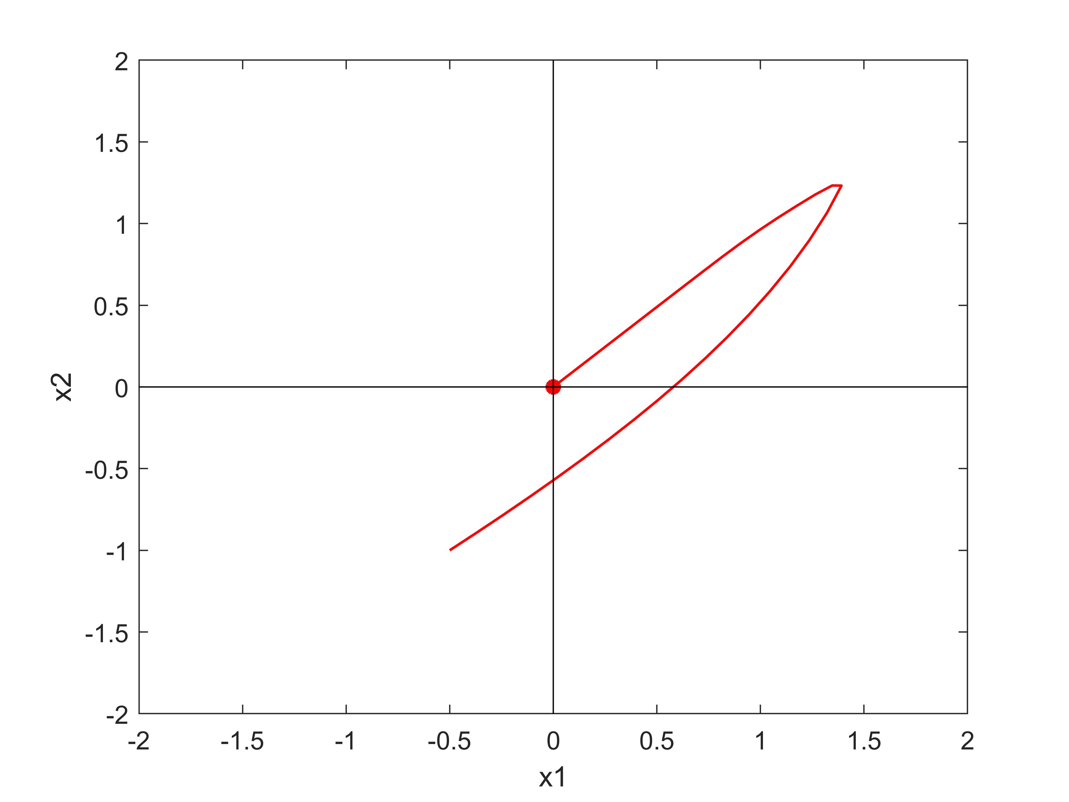
(a) Trajectory of the solution

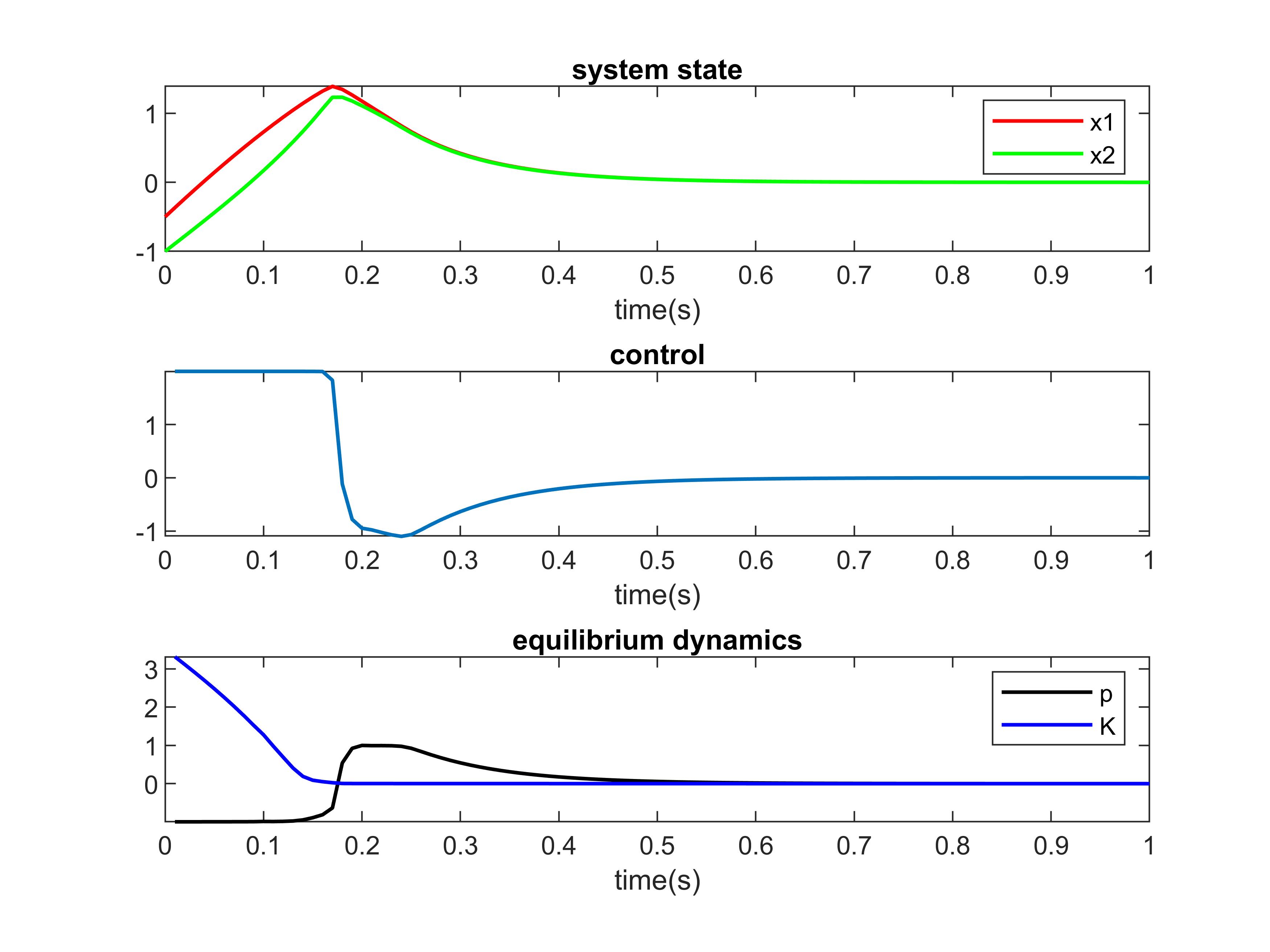
(b) Time history of the solution

Figure 2: Affine DVI

In the affine DVI example, the solution clearly identifies the optimized trajectory as shown in Fig.2, which includes four modes without any predefined sequence:

• from $0s$ to $0.14s$, mode $p=l,w\geq 0$ occurs;

• from $0.14s$ to $0.20s$, mode $p\in(l,u),w=0$ occurs;

• from $0.20s$ to $0.24s$, mode $p=u,w\leq 0$ occurs;

• from $0.24s$ to $1s$, mode $p\in(l,u),w=0$ occurs.

(a) Trajectory of the solution

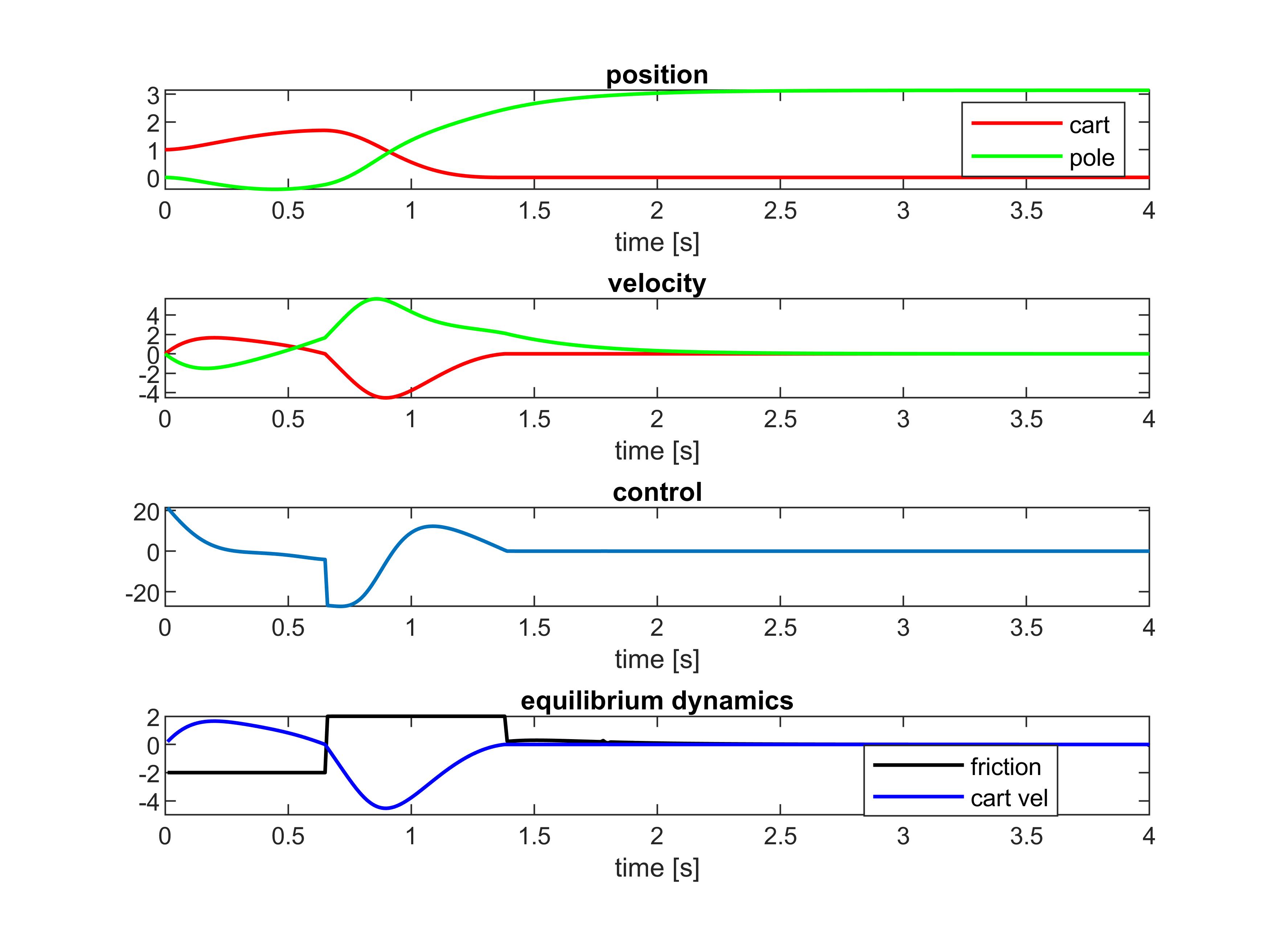
(b) Time history of the solution

Figure 3: Cart pole with friction

In the cart pole with friction example, the Coulomb friction introduces the mode switching between stick and sliding behaviours. As shown in Fig.3, the solution includes three modes without any predefined sequence:

• from $0s$ to $0.65s$, cart slides to right side;

• from $0.65s$ to $1.38s$, cart slides to left side;

• from $1.38s$ to $4s$, cart sticks and keeps the pole balance.

(a) Trajectory of the solution

(b) Time history of the state and control

(c) Time history of the equilibrium dynamics

Figure 4: 2D hopper with multiple jump gaits

In the 2D hopper example shown in Fig.4, jump motion with multiple gaits can be discovered without any predefined sequence. This solution includes ten modes that can be classified into stick and flight phase:

• stick phase: hopper sticks to the ground and is subjected to the impact force and Coulomb friction. Here, the stick phase occurs over time intervals [0s, 0.03s], [0.16s, 0.32s], [0.50s, 0.87s], [0.95s, 1.06s] and [1.17s, 1.8s];

• flight phase: hopper jumps off the ground and is not subjected to any contact force. Here, the flight phase occurs over time intervals [0.03s, 0.16s], [0.32, 0.50s], [0.87s, 0.95s], [1.06s, 1.17s] and [1.8s, 2s].

5.4 Sensitivity of Solver Performance

In this subsection, we investigate the sensitivity of the solver performance to the ill-posedness of the feasible region using an affine DVI example. Regarding the solver robustness, as shown in Table 2, NIP1 is as robust as IP for handling all randomly generated initial guesses for different $s^{*}$, while NIP2 is also sufficiently robust in this affine case.

Regarding the average number of iterations required to obtain a solution, as shown in Fig. 5(a), two major conclusions underlining the advantages of the proposed method can be stated. First, for a given $s^{*}$, both NIP1 and NIP2 can converge to a solution with significantly fewer iterations compared to the IP. Second, as the decrease of $s^{*}$, NIP1 does not significantly increase the number of iterations, that is, it is less sensitive to the ill-posedness of the primal feasible region. By contrast, IP requires many more iterations when the given $s^{*}$ is sufficiently small. In addition, it is also observed that NIP2 requires more iterations when specifying a perturbed parameter for the middle accuracy ($s^{*}=10^{-4},10^{-5},10^{-6}$), while recovers to the need of fewer iterations when specifying a perturbed parameter for the high accuracy ($s^{*}=10^{-7},10^{-8}$), we provide an explanation at the end of this subsection.

Regarding the average computation time to obtain a solution, as shown in Fig. 5(b), although NIP1 needs significantly fewer iterations, this advantage does not be transformed into a distinct advantage in computation time. This is mainly because of the code efficiency where the current version of the proposed solver is developed based on the Matlab built-in dense (full) matrix, whereas IPOPT via CasADi interface is based on the Matlab built-in sparse matrix which leads to a dramatic improvement in execution time. However, a significant improvement in the computation efficiency can be expected if employing the C code generation and the stage-wise parallel computation for the functions and derivatives evaluation. Finally, note that NIP2 requires much more time, particularly for middle accuracy cases. The reason for this observation is that NIP2 frequently calls FRP to facilitate the progress to solution, especially in the first several iterations, whereas FRP is a time-consuming routine in the current version of proposed solver where an optimization problem is solved.

The simulation results for NIP1 and NIP2 indicate that some shortcomings of the NIP method that may be magnified in the discretized OCPEC, can be significantly alleviated by the continuation method. Specifically, the NIP method may suffer numerical difficulties if the FB function value can not be sufficiently decreased to ensure that the inequality constraints are satisfied. This can be caused by many kinds of problematic situations, such as poor initial guess or some special feasible regions (e.g., the middle accuracy cases in this example).

Table 2: Number of Success Case

$s^{*}$	NIP1	NIP2	IP
$10^{-3}$	100	100	100
$10^{-4}$	100	96	100
$10^{-5}$	100	98	100
$10^{-6}$	100	96	100
$10^{-7}$	100	95	100
$10^{-8}$	100	96	100

(a) Number of iterations

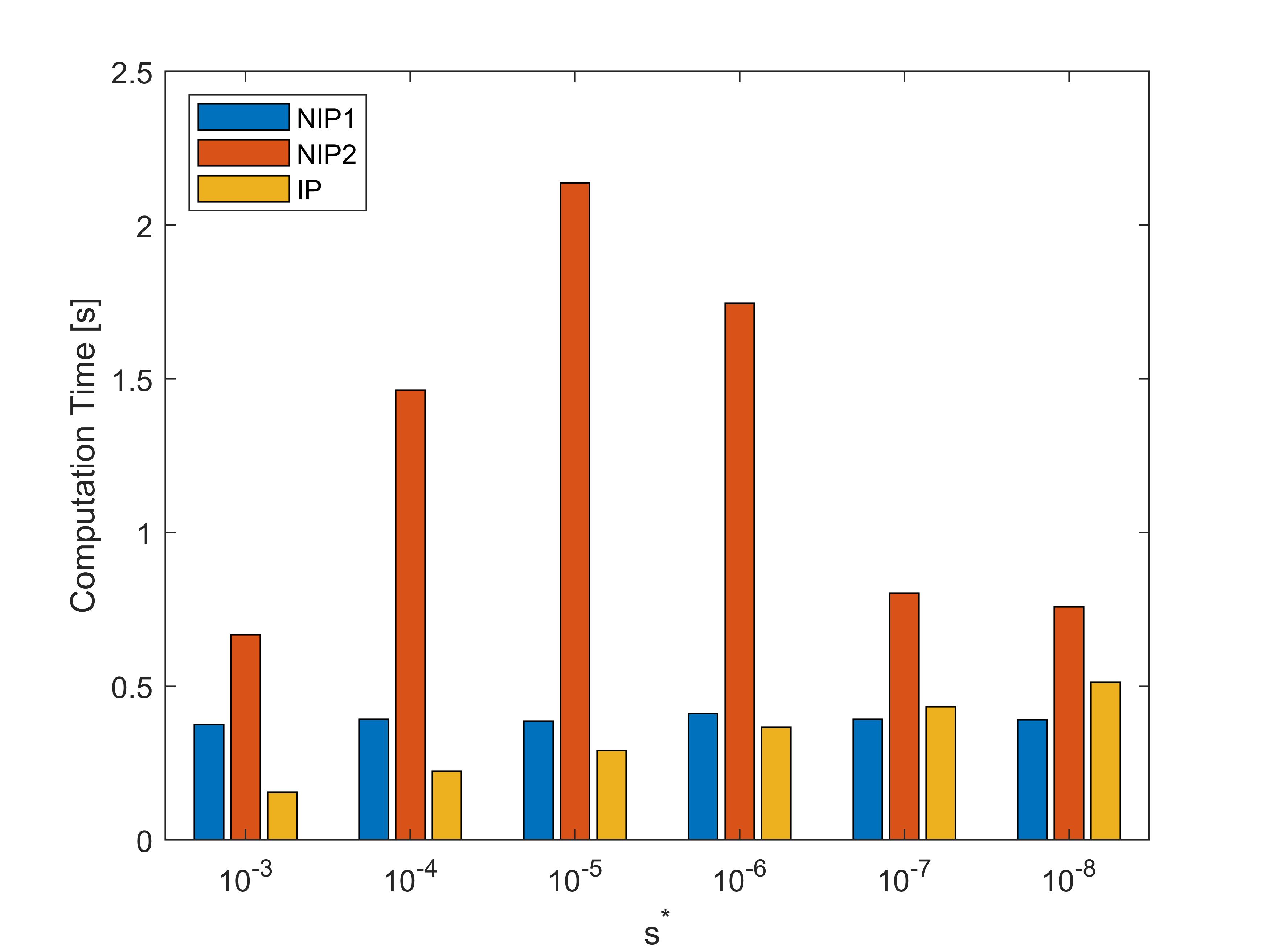
(b) Computation time

Figure 5: Sensitivity of solver performance

5.5 Solution Quality

In this subsection, we investigate the quality of the optimal solutions found by NIP1 and IP using two nonlinear CITO examples. Regarding the minimum cost function value, as shown in Table 6, in these two examples, NIP1 can always find a solution with a smaller cost function value than that obtained by IP for all desired $s^{*}$, mainly benefiting from a larger stepsize and search space. Regarding the maximum constraint satisfaction, as shown in Table 6 - 6, IP has better constraint satisfaction owing to the excessive enforcement of feasibility by the fraction-to-the-boundary rules. Note that even though the proposed method does not enforce the iterates to strictly remain in the feasible region, the inequality constraints are satisfied reasonably well.

Table 3: Minimum Cost Function Value

	Cart Pole		Hopper
$s^{*}$	NIP1	IP	NIP1	IP
$10^{-3}$	644.097	2442.652	10.003	24.118
$10^{-5}$	631.396	2442.968	10.632	19.723
$10^{-7}$	633.782	2442.970	9.863	24.011

Table 4: Maximum Constraint Violation ($r_{eq}$)

	Cart Pole		Hopper
$s^{*}$	NIP1	IP	NIP1	IP
$10^{-3}$	3.750e-06	9.077e-10	3.375e-05	1.499e-07
$10^{-5}$	5.334e-05	1.217e-10	9.954e-05	1.032e-07
$10^{-7}$	3.427e-05	3.993e-12	8.138e-05	4.388e-08

Table 5: Maximum Constraint Violation ($r_{ineq}$)

	Cart Pole		Hopper
$s^{*}$	NIP1	IP	NIP1	IP
$10^{-3}$	5.658e-04	0.000e+00	2.671e-03	2.850e-09
$10^{-5}$	4.631e-04	0.000e+00	9.544e-05	0.000e+00
$10^{-7}$	2.076e-04	0.000e+00	6.568e-04	3.860e-09

Table 6: Maximum Constraint Violation ($r_{comp}$)

	Cart Pole		Hopper
$s^{*}$	NIP1	IP	NIP1	IP
$10^{-3}$	1.433e-03	9.918e-04	2.671e-03	9.841e-04
$10^{-5}$	1.059e-03	6.429e-06	1.551e-04	8.614e-06
$10^{-7}$	4.664e-04	6.002e-08	1.359e-04	7.156e-08

6 Conclusion

In this study, we proposed a non-interior-point continuation method for solving OCPEC. The proposed method leverages the regularization reformulation for equilibrium constraints to mitigate the numerical difficulties caused by the violation of CQs. Under the framework of the continuation method, a dedicated NLP solver using the smooth FB function to treat the inequality constraints is employed. Several numerical techniques are designed to enhance the performance of the proposed solver. The local convergence and solution error were analyzed. We demonstrated the effectiveness of the proposed algorithm through several practical examples. Numerical experiments have underlined that, compared with an interior-point solver, the proposed solver can find a better solution, is less sensitive to the ill-posedness of the feasible region, and has a faster convergence performance in terms of the number of iterations.

Future research can be classified into the following two categories. Regarding theoretical research, we wish to investigate the approximation error, which was briefly discussed in Remark 1. This may help us to leverage some sophisticated integration methods so that a larger $\Delta t$ can be selected to generate a smaller size NLP problem. Regarding practical applications, we are considering the embedded application of the proposed solver on a quadruped and attempting to utilize the DVI to formulate more complex switch behaviors (e.g., periodic gaits). In addition, owing to the larger search space and the insensitivity to the change in perturbed parameters, the proposed solver can be easily warm-started and has a rapid convergence, which makes it promising for model predictive control. However, because most of the intermediate iterates are infeasible, the proposed solver does not allow for adopting the early termination to return a sub-optimal but feasible solution unless some additional steps (e.g. the projection step) are introduced to enforce the feasibility. Therefore, a warm-start strategy with a feasibility guarantee will be investigated in the future.

References

- [1] V. Acary and B. Brogliato. Numerical Methods for Nonsmooth Dynamical Systems: Applications in Mechanics and Electronics. Springer Science & Business Media, 2008.
- [2] J.A.E. Andersson, J. Gillis, Horn G., J.B. Rawlings, and M. Diehl. CasADi: a software framework for nonlinear optimization and optimal control. Mathematical Programming Computation, 11(1):1–36, 2019.
- [3] F. Benita and P. Mehlitz. Bilevel optimal control with final-state-dependent finite-dimensional lower level. SIAM Journal on Optimization, 26(1):718–752, 2016.
- [4] H.Y. Benson, D.F. Shanno, and R.J. Vanderbei. Interior-point methods for nonconvex nonlinear programming: Complementarity constraints. Operations Research and Financial Engineering, pages 1–20, 2002.
- [5] J.V. Burke, F.E. Curtis, A.S. Lewis, M.L. Overton, and L.E.A. Simões. Gradient sampling methods for nonsmooth optimization. Numerical Nonsmooth Optimization, pages 201–225, 2020.
- [6] B. Chen, X. Chen, and C. Kanzow. A penalized Fischer-Burmeister NCP-function. Mathematical Programming, 88(1):211–216, 2000.
- [7] B. Chen and P.T. Harker. A non-interior-point continuation method for linear complementarity problems. SIAM Journal on Matrix Analysis and Applications, 14(4):1168–1190, 1993.
- [8] C. Chen and O.L. Mangasarian. A class of smoothing functions for nonlinear and mixed complementarity problems. Computational Optimization and Applications, 5(2):97–138, 1996.
- [9] X. Chen and Z. Wang. Differential variational inequality approach to dynamic games with shared constraints. Mathematical Programming, 146(1):379–408, 2014.
- [10] S. Cleac’h, T. Howell, M. Schwager, and Z. Manchester. Fast contact-implicit model-predictive control. arXiv preprint, 2021.
- [11] S.P. Dirkse and M.C. Ferris. The path solver: a nommonotone stabilization scheme for mixed complementarity problems. Optimization Methods and Software, 5(2):123–156, 1995.
- [12] F. Facchinei and J.-S. Pang. Finite-Dimensional Variational Inequalities and Complementarity Problems. Springer, 2003.
- [13] M.C. Ferris, S.P. Dirkse, and A. Meeraus. Mathematical programs with equilibrium constraints: automatic reformulation and solution via constrained optimization. In Frontiers in Applied General Equilibrium Modeling, pages 67–93. Cambridge University Press, 2005.
- [14] A. Fischer. A special Newton-type optimization method. Optimization, 24(3-4):269–284, 1992.
- [15] L. Guo and J.J. Ye. Necessary optimality conditions for optimal control problems with equilibrium constraints. SIAM Journal on Control and Optimization, 54(5):2710–2733, 2016.
- [16] T. Hoheisel, C. Kanzow, and A. Schwartz. Theoretical and numerical comparison of relaxation methods for mathematical programs with complementarity constraints. Mathematical Programming, 137(1):257–288, 2013.
- [17] K. Hotta and A. Yoshise. Global convergence of a class of non-interior point algorithms using Chen-Harker-Kanzow-Smale functions for nonlinear complementarity problems. Mathematical Programming, 86:105–133, 1999.
- [18] T. Howell, S. Cleac’h, S. Singh, P. Florence, Z. Manchester, and V. Sindhwani. Trajectory optimization with optimization-based dynamics. IEEE Robotics and Automation Letters, 7(3):6750–6757, 2022.
- [19] A.F. Izmailov and M.V. Solodov. An active-set Newton method for mathematical programs with complementarity constraints. SIAM Journal on Optimization, 19(3):1003–1027, 2008.
- [20] H. Jiang and D. Ralph. Smooth SQP methods for mathematical programs with nonlinear complementarity constraints. SIAM Journal on Optimization, 10(3):779–808, 2000.
- [21] C. Kanzow. Some noninterior continuation methods for linear complementarity problems. SIAM Journal on Matrix Analysis and Applications, 17(4):851–868, 1996.
- [22] S. Leyffer, G. López-Calva, and J. Nocedal. Interior methods for mathematical programs with complementarity constraints. SIAM Journal on Optimization, 17(1):52–77, 2006.
- [23] D. Li and M. Fukushima. Smoothing Newton and quasi-Newton methods for mixed complementarity problems. Computational Optimization and Applications, 17(2):203–230, 2000.
- [24] D. Liao-McPherson, M. Huang, and I. Kolmanovsky. A regularized and smoothed Fischer-Burmeister method for quadratic programming with applications to model predictive control. IEEE Transactions on Automatic Control, 64(7):2937–2944, 2018.
- [25] D. Liao-McPherson and I. Kolmanovsky. FBstab: a proximally stabilized semismooth algorithm for convex quadratic programming. Automatica, 113:108801, 2020.
- [26] K Lin and T. Ohtsuka. A non-interior-point method for the optimal control problem with equilibrium constraints. In Proceedings of the 61st IEEE Conference on Decision and Control, pages 1–7, Cancun, Mexico, 2022.
- [27] I. Mynttinen, A. Hoffmann, E. Runge, and P. Li. Smoothing and regularization strategies for optimization of hybrid dynamic systems. Optimization and Engineering, 16(3):541–569, 2015.
- [28] J. Nocedal and S.J. Wright. Numerical Optimization. Springer, 2006.
- [29] A. Nurkanović, S. Albrecht, B. Brogliat, and M. Diehl. The time-freezing reformulation for numerical optimal control of complementarity lagrangian systems with state jumps. arXiv preprint, 2021.
- [30] A. Nurkanović and M. Diehl. NOSNOC: a software package for numerical optimal control of nonsmooth systems. IEEE Control Systems Letters, 2022.
- [31] J. Outrata, M. Kocvara, and J. Zowe. Nonsmooth Approach to Optimization Problems with Equilibrium Constraints: Theory, Applications and Numerical Results, volume 28. Springer Science & Business Media, 2013.
- [32] J.-S. Pang and D.E. Stewart. Differential variational inequalities. Mathematical Programming, 113(2):345–424, 2008.
- [33] J.-S. Pang and D.E. Stewart. Solution dependence on initial conditions in differential variational inequalities. Mathematical Programming, 116(1):429–460, 2009.
- [34] M. Posa, C. Cantu, and R. Tedrake. A direct method for trajectory optimization of rigid bodies through contact. International Journal of Robotics Research, 33(1):69–81, 2014.
- [35] L. Qi and D. Sun. Improving the convergence of non-interior point algorithms for nonlinear complementarity problems. Mathematics of Computation, 69(229):283–304, 1999.
- [36] A.U. Raghunathan and L.T. Biegler. An interior point method for mathematical programs with complementarity constraints (MPECs). SIAM Journal on Optimization, 15(3):720–750, 2005.
- [37] D. Ralph and S.J. Wright. Some properties of regularization and penalization schemes for MPECs. Optimization Methods and Software, 19(5):527–556, 2004.
- [38] H. Scheel and S. Scholtes. Mathematical programs with complementarity constraints: stationarity, optimality, and sensitivity. Mathematics of Operations Research, 25(1):1–22, 2000.
- [39] S. Scholtes. Convergence properties of a regularization scheme for mathematical programs with complementarity constraints. SIAM Journal on Optimization, 11(4):918–936, 2001.
- [40] D.E. Stewart. Uniqueness for index-one differential variational inequalities. Nonlinear Analysis: Hybrid Systems, 2(3):812–818, 2008.
- [41] D.E. Stewart and M. Anitescu. Optimal control of systems with discontinuous differential equations. Numerische Mathematik, 114(4):653–695, 2010.
- [42] D.E. Stewart and J.C. Trinkle. An implicit time-stepping scheme for rigid body dynamics with inelastic collisions and coulomb friction. International Journal for Numerical Methods in Engineering, 39(15):2673–2691, 1996.
- [43] D. Sun and J. Han. Newton and quasi-Newton methods for a class of nonsmooth equations and related problems. SIAM Journal on Optimization, 7(2):463–480, 1997.
- [44] A. Vieira, B. Brogliato, and C. Prieur. Quadratic optimal control of linear complementarity systems: first-order necessary conditions and numerical analysis. IEEE Transactions on Automatic Control, 65(6):2743–2750, 2020.
- [45] A. Wächter and L.T. Biegler. On the implementation of an interior-point filter line-search algorithm for large-scale nonlinear programming. Mathematical Programming, 106(1):25–57, 2006.
- [46] R.A. Waltz, J. Morales, J. Nocedal, and D. Orban. An interior algorithm for nonlinear optimization that combines line search and trust region steps. Mathematical Programming, 107:391–408, 2006.