Training set cleansing of backdoor poisoning by self-supervised representation learning

Abstract

A backdoor or Trojan attack is an important type of data poisoning attack against deep neural network (DNN) classifiers, wherein the training dataset is poisoned with a small number of samples that each possess the backdoor pattern (usually a pattern that is either imperceptible or innocuous) and which are mislabeled to the attacker’s target class. When trained on a backdoor-poisoned dataset, a DNN behaves normally on most benign test samples but makes incorrect predictions to the target class when the test sample has the backdoor pattern incorporated (i.e., contains a backdoor trigger). Here we focus on image classification tasks and show that supervised training may build stronger association between the backdoor pattern and the associated target class than that between normal features and the true class of origin. By contrast, self-supervised representation learning ignores the labels of samples and learns a feature embedding based on images’ semantic content. Using a feature embedding found by self-supervised representation learning, a data cleansing method, which combines sample filtering and re-labeling, is developed. Experiments on CIFAR-10 benchmark datasets show that our method achieves state-of-the-art performance in mitigating backdoor attacks.

Index Terms—  Backdoor; contrastive learning; data cleansing

1 Introduction

It has been shown that Deep Neural Networks (DNNs) are vulnerable to backdoor attacks (Trojans) [1]. Such an attack is launched by poisoning a small batch of training samples from one or more source classes chosen by the attacker. Training samples are poisoned by embedding innocuous or imperceptible backdoor patterns into the samples and changing their labels to a target class of the attack. For a successful attack, a DNN classifier trained on the poisoned dataset: i) will have good accuracy on clean test samples (without backdoor patterns incorporated); ii) but will classify test samples that come from a source class of the attack, but with the backdoor pattern incorporated (i.e., backdoor-triggered), to the target class. Backdoor attacks may be relatively easily achieved in practice because of an insecure training out-sourcing process, through which both a vast training dataset is created and deep learning itself is conducted. Thus, devising realistic defenses against backdoor poisoning is an important research area. In this paper, we consider defenses that operate after the training dataset is formed but before the training process. The aim is to cleanse the training dataset prior to training of the classifier.

We observe that, with supervised training on the backdoor-attacked dataset, a DNN model learns stronger “affinity” between the backdoor pattern and the target class than that between normal features and the true class of origin. This strong affinity is enabled (despite the backdoor pattern typically being small in magnitude) by mislabeling the poisoned samples to the target class. However, self-supervised contrastive learning, does not make use of supervising class labels; thus, it provides a way for learning from the training set without learning the backdoor mapping.

Based on this observation, a training set cleansing method is proposed. Using the training set $\mathcal{D}$, we first learn a feature representation using self-supervised contrastive loss. We hypothesize that, since the backdoor pattern is small in magnitude, self-supervised training will not emphasize the features of the backdoor pattern contained in the poisoned samples. Working in the learned feature embedding space, we then propose two methods (kNN-based and Energy based) to detect and filter out samples whose predicted class is not in agreement with the labeled class. We then relabel detected samples to their predicted class (for use in subsequent classifier training) if the prediction is made “with high confidence”. An overview of our method is shown in Fig. 1. Unlike many existing backdoor defenses, Our method requires neither a small clean dataset available to the defender, nor a reverse-engineered backdoor pattern (if present), nor a fully trained DNN classifier on the (possibly poisoned) training dataset. Also, ours is the first work to address the problem of backdoor samples evading (“leaking through”) a rejection filter – we propose a relabeling method to effectively neutralize this effect. A complete version of our paper with Appendix is online available.

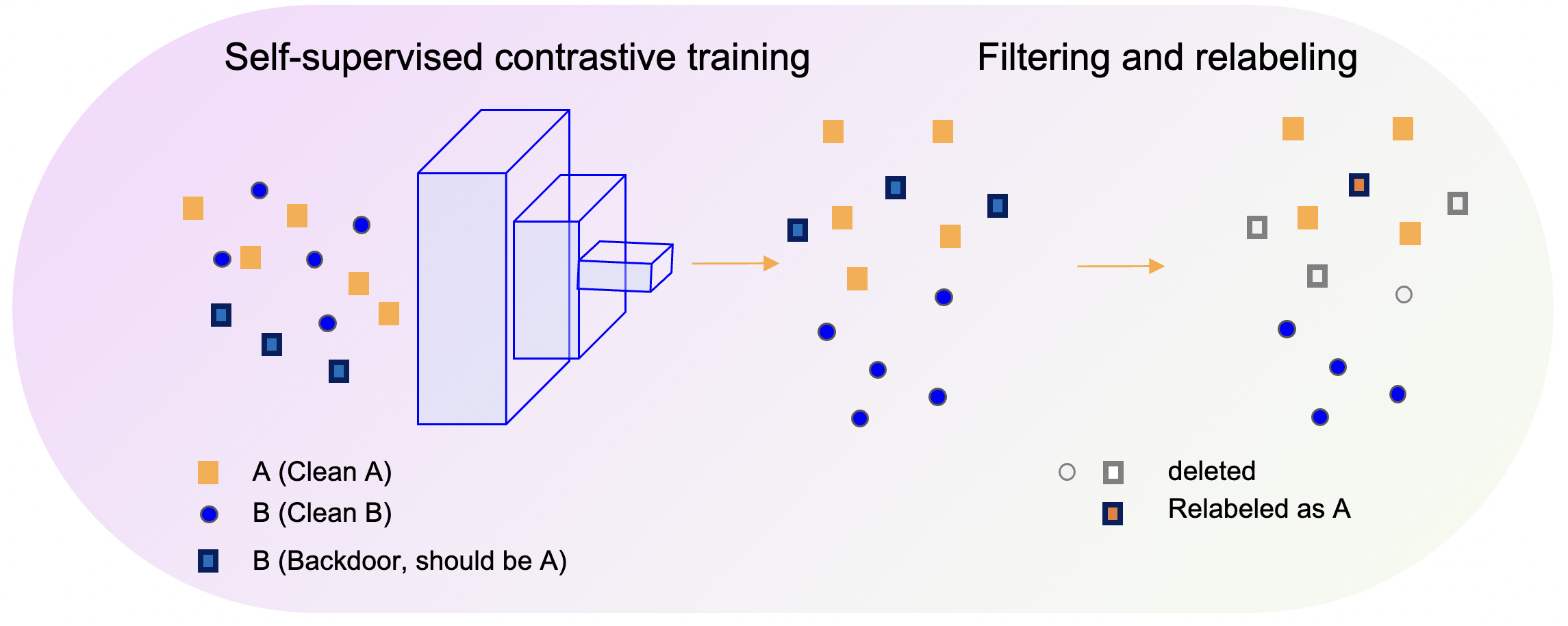
Fig. 1: Overview of the data cleansing method.

2 Threat model and related works

Consider a clean dataset ${\mathcal{D}}=\{(x_{i},y_{i})~{}|~{}i=1...N\}$, where: $x_{i}\in{\mathbb{R}}^{X\times H\times W}$ is the $i^{\rm th}$ image in the dataset with $X$, $H$ and $W$ respectively the number of image channels, height, and width; $y_{i}\in\{1,2,...,C\}$ is the corresponding class label, with the number of classes $C>1$. Backdoor attacks poison a dataset by: i) choosing an attack target class $t$, and then obtaining a subset (of size $M$) of images from classes other than $t$: ${\mathcal{D}}_{s}=\{(x_{j},y_{j})|i=1...M,y_{j}\neq t\}$, ${\mathcal{D}}_{s}\subset{\mathcal{D}}$, and $M\ll N$; ii) the backdoor pattern is then incorporated into each sample in ${\mathcal{D}}_{s}$ using the attacker’s backdoor embedding function $g:{\mathbb{R}}^{X\times H\times W}\xrightarrow{}{\mathbb{R}}^{X\times H\times W}$; iii) the label for each poisoned sample is then changed to the target class: ${\mathcal{D}}_{p}=\{(g(x),t)|x\in{\mathcal{D}}_{s}\}$; iv) finally the poisoned dataset is formed by putting the attacked images back into the training set: $\bar{{\mathcal{D}}}=({\mathcal{D}}\backslash{\mathcal{D}}_{s})\cup{\mathcal{D}}_{p}$. If the attack is successful, the victim model $f:{\mathbb{R}}^{X\times H\times W}\rightarrow\{1,2,...,C\}$, when trained on the poisoned dataset, will have normal (good) classification accuracy on clean (backdoor-free) test samples, but will classify most backdoor-triggered test samples to the target class of the attack. In the image domain, backdoor patterns could, e.g., be: i) a small patch that replaces the original pixels of an image [1, 2, 3]; ii) a perturbation added to some pixels of an image [4, 5, 6]; or iii) a “blended” patch attack [4].

On the other hand, the defender aims to obtain a classifier with good classification accuracy on clean test samples and which correctly classifies test samples with the backdoor pattern. Defenses against backdoors that are deployed post-training aim to detect whether a DNN model is a backdoor victim [2, 7, 8, 9, 6, 10] and, further, to mitigate the attack if a detection is declared [2, 11, 12]. Most post-training defenses require a relatively small clean dataset (distributed as the clean training set), with their performance generally sensitive to the number of available clean samples [12, 2, 7, 10]. In this paper, alternatively, we aim to cleanse the training set prior to deep learning. Related work on training set cleansing includes [13, 14, 15, 16]. All of these methods rely on embedded feature representations of a classifier fully trained on the possibly poisoned training set ([14] suggests that an auto-encoder could be used instead). [14, 13] use a 2-component clustering approach to separate backdoor-poisoned samples from clean samples ([14] uses a singular-value decomposition while [13] uses a simple 2-means clustering), while [15] uses a Gaussian mixture model whose number of components is chosen based on BIC [17]. Instead of clustering, [16] employs a reverse-engineered backdoor pattern estimated using a small clean dataset. DBD [18] builds a classifier based on an encoder learned via self-supervised contrastive loss; then the classifier is fine-tuned. In each iteration some samples are identified as “low credible” samples by the classifier, with their labels removed; the classifier is then updated based on the processed dataset in a semi-supervised manner.

3 Methodology

3.1 Vulnerability of supervised training

We now illustrate the vulnerability of supervised training by analysis of a simple linear model trained on a poisoned dataset, considering the case where all classes other than the target are (poisoned) source classes. The victim classifier forms a linear discriminant function for each class $s$, i.e., the inner product $f_{s}(x)=x\cdot w_{x}$, where $w_{s}\in{\mathbb{R}}^{X\times H\times W}$ is the vector of model weights corresponding to class $s$. Assume that, after supervised training, each training sample is classified correctly with confidence at least $\tau>0$ as measured by the margin:

$$f_{y_{i}}(x_{i})-\max_{c\neq y_{i}}f_{c}(x_{i})\geq\tau,~{}~{}\forall(x_{i},y_{i})\in\bar{{\mathcal{D}}}.\vspace{-0.1in}$$ (1)

Assuming that the backdoor pattern $\Delta x$ is additively incorporated, given an attack sample based on clean $x_{s}$ originally from source-class $s\not=t$, Eq. (1) implies

$$w_{t}\cdot(x_{s}+\Delta x)-w_{s}\cdot(x_{s}+\Delta x)\geq\tau.\vspace{-0.05in}$$ (2)

If $x_{s}$ is also classified to $s$ with margin $\tau$, then

$$w_{s}\cdot x_{s}-w_{t}\cdot x_{s}\geq\tau.\vspace{-0.07in}$$ (3)

Adding (1) and (3) gives

$$f_{t}(\Delta x)-f_{s}(\Delta x)=(w_{t}-w_{s})\cdot\Delta x\geq 2\tau.\vspace{-0.05in}$$ (4)

This loosely suggests that, after training with a poisoned training dataset, the model has stronger “affinity” between the target class and the backdoor pattern (4) than between the source class and the class-discriminative features of clean source-class samples (3). This phenomenon is experimentally verified when the model is a DNN, as shown in Apdx. A.

However, these strong affinities are only made possible by the mislabeling of the backdoor-poisoned samples. Given that usually the perturbation $\Delta x$ is small, backdoor attacked images differ minutely from the original (clean) images. Thus if a model is trained in a self-supervised manner, without making use of the class labels, the feature representations of $x$ and $x+\Delta x$ should be quite similar/highly proximal. Thus, in the model’s representation space, poisoned samples may “stand out” as outliers in that their labels may disagree with the labels of samples in close proximity to them. This is the basic idea behind the cleansing method we now describe.

3.2 Self-supervised contrastive learning

SimCLR [19, 20] is a self-supervised training method to learn a feature representation for images based on their semantic content. In SimCLR, in each mini-batch, $K$ samples are randomly selected from the training dataset, and each selected sample $x_{k}$ is augmented to form two versions, resulting in $2K$ augmented samples. Augmented samples are then fed into the feature representation model, which is an encoder $E(\cdot)$ followed by a linear projector $L(\cdot)$, with the feature vector $z$ extracted from the last layer: $z=L(E(x))$. For simplicity we will refer to $L(E(\cdot))$ as the “encoder” hereon. The encoder is trained to minimize the following objective function:

$$C=-\frac{1}{2K}\sum_{i=1}^{2K}\log\frac{\exp{(z_{i}\cdot z_{\alpha(i)}/\tau})}{\sum_{i^{\prime}=1,~{}i^{\prime}\neq i}^{2K}\exp{(z_{i}\cdot z_{i^{\prime}}/\tau})},\vspace{-0.05in}$$ (5)

where $i$ and $\alpha(i)$ are indexes of two samples augmented from the same training sample. Consistent with minimizing (5), SimCLR trains the encoder by projecting an image and its augmentations to similar locations in the derived feature space. So, given the fact that a backdoor attack makes minor changes to a poisoned training sample while preserving the semantic content related to its source class (the label of the clean sample), it is expected that the encoder will learn to project a backdoor image into a feature space location close to clean (and augmented) images from the source class. Working in the feature representation space learned by SimCLR, a training-sample filtering and re-labeling method can thus be deployed to cleanse the training set.

3.3 Data filtering

We consider two options for data filtering: k Nearest Neighbor (kNN) classifier and class-based “energy” score.

kNN: kNN is a widely used classification model. The class of a sample is determined by the voting of its top k nearest samples in the derived feature space. Basically we want to leverage the SimCLR representations and compare the label of a data point in the training set with the labels of nearby data points in representation space to verify the class label. The class label of a training sample is accepted if its labeled class agrees with kNN’s predicted class (based on plurality voting); otherwise it is likely to be mislabelled/attacked and will be rejected. In our experiments, $k$ is chosen to be half of the number of images from each of the classes.

Energy: Given a sample (in the embedded feature space) $z_{i}$, an energy score corresponding to class $c$ is as follows:

$$S_{c}(z_{i})=\log\frac{1}{|{\mathcal{I}}_{c}\backslash\{i\}|}\sum_{k\in{\mathcal{I}}_{c}\backslash\{i\}}\frac{\exp(z_{i}\cdot z_{k}/\tau)}{\sum_{k^{\prime}=1,k^{\prime}\not=i}^{N}\exp(z_{i}\cdot z_{k^{\prime}}/\tau)},$$ (6)

where ${\mathcal{I}}=\{i~{}|~{}i=1...N\}$ is the set of indices of all the samples in the training set and ${\mathcal{I}}_{c}=\{i~{}|~{}i\in{\mathcal{I}},y_{i}=c\}$ is the set of indices of samples from class $c$. A class decision can be made based on a sample’s class-conditional scores: $c^{*}(z_{i})=\operatorname*{arg\,max}_{c}S_{c}(z_{i})$. A training sample is accepted only if its predicted class $c^{*}(z_{i})$ agrees with its class label.

Tab. 1 shows the performance of Energy and kNN filtering methods using the ResNet-18 encoder architecture on the CIFAR-10 dataset, when 1000 samples are poisoned. Our filtering method can filter out 97% of backdoor samples while keeping most of the clean samples. However, the leaking of even a few backdoor samples is still problematic – [1] shows that even 50 backdoor samples for the CIFAR-10 dataset can make the attack successful. So one cannot successfully defend backdoor attacks only by data filtering.

	clean	backdoor
Energy	89.14	2.9
kNN	88.95	3.2

Table 1: The percentage of clean and backdoor images remaining after filtering methods applied.

3.4 Re-labeling

From the discussion in Sec. 3.2, SimCLR projects a backdoor image to a feature space location close to clean images from the source class. For a sample that is rejected with a certain level of confidence (e.g., for KNN, if all $k$ neighbors are labeled to class 1, but the sample is labeled to class 2), it is likely that the sample is a backdoor image and that the predicted class is the source class. Also, [2] indicates that a backdoor attack can be unlearned if a model is trained on images with backdoor triggers but labeled to the true class. Thus, to neutralize the influence of the backdoor images leaked in the filtering step, we first identify samples that are rejected (samples with kNN/energy’s predictions do not agree with their class labels) with a confidence threshold $T$. Then we re-label these samples to the predicted class. For kNN, the confidence can be measured by the fraction of samples with the predicted label amongst the $K$ nearest neighbors; for the energy-based method, the maximum score (over all classes) can be used as the confidence measure. Note that $T$ is a hyper-parameter – the performance of our relabeling method is sensitive to the threshold $T$. Care should be taken when a sample is relabeled since it inevitably induces label noise–the predictions of kNN and the energy-based method are not always reliable. So it is not a good idea to pre-define a number/ratio of samples that will be relabeled given that the number of backdoor attacked samples is not known. Alternatively, the confidence can be determined based on the confidence of clean samples (here we treat all accepted samples in the filtering step as clean samples). In practice, we set the threshold as the 80-th percentile of the confidences of accepted samples.

4 Experiments

Our experiments are mainly conducted on CIFAR-10 [21]. Two global backdoor patterns (additive [6] and WaNet [22]) and two local patterns (BadNet[1], blended[4]) are considered in our work. The details of those attacks can be found in Apdx. C. For all the experiments ResNet-18 is used as the model architecture. A ResNet-18 encoder is first trained for 1000 epochs on the given dataset using the SimCLR loss (Eq. 5); then the kNN or energy based filtering and relabeling are applied to clean the dataset. Finally, the classifier is trained on the cleaned dataset using Supervised contrastive loss (SupCon) [20]. The performance of a defense is evaluated by two measures: clean test accuracy (ACC) and attack success rate (ASR). Our method is compared with three baseline methods: DBD[18], Activation Clustering (AC)[13], and Spectral Signature (SS) [14]. AC and SS train a ResNet-18 classifier on the poisoned dataset and then identify backdoor samples using the classifier’s internal layer activations, by activation clustering (AC) or by checking if there are abnormally large activations (SS). Notably both AC and SS assume knowledge of the attacker’s target class, and SS further assumes the number of poisoned images is known. After filtering, a new classifier is trained on the cleaned dataset using SupCon. DBD defends backdoor attacks by iteratively identifying backdoor images using a classifier (pre-trained using SimCLR at the beginning) and then fine-tuning the classifier using a semi-supervised loss (MixMatch [23]), treating the backdoor images as unlabeled data and clean images as labeled data. The methods mentioned above require careful adjusting of hyper-parameters to get good performance; by contrast, there is only one hyper-parameter in our method (the threshold $T$ in the relabeling step), which can be automatically set based on the confidence on accepted samples, as discussed above.

	Additive		BadNet		blend		WaNet
	ASR	ACC	ASR	ACC	ASR	ACC	ASR	ACC
None	99.9	94.14	98.4	94.19	99.9	94.14	67.6	93.11
AC[13]	100	92.75	3.2	94.49	1.7	94.50	68.9	87.05
SS[14]	97.4	91.14	3.2	94.49	49.9	94.36	63.5	93.04
DBD	0.7	92.57	1.5	91.49	1.4	91.89	0.7	91.65
kNN	2.6	91.46	4.2	92.37	4.2	92.13	3.6	92.24
Energy	2.8	91.91	4.9	92.12	2.5	92.10	1.3	91.25

Table 2: ASR (%) and ACC (%) for our methods and comparison methods under different attacks.

Performance: The defense methods aim to achieve high ACC and low ASR. Tab. 2 shows the performance of different methods when the number of poisoned images is 1000 for additive, BadNet, and blend attacks and 5000 for the WaNet attack. AC performs well for local backdoor attacks (BadNet and blend) where a backdoor image contains mostly features from the source class (original class before attack), i.e. such that the internal layer features of the classifier are different from those of clean target class images; but when the pattern is global (additive and WaNet) the classifier trained on the poisoned data can project images with backdoor patterns into locations close to those of clean target class samples; thus the performance for these attacks is poor. Similarly, SS performs well only on BadNet and can mitigate the ASR for the blended attack, but does not work well on additive and WaNet attacks. Our method and DBD give comparable performance; however Fig. 2 shows that, with an increased number of poisoned images, DBD fails (ASR close to 100% and drop of ACC under the additive attack). The likely reason is the iterative filtering of DBD – in any iteration, if some backdoor samples are falsely identified as clean, the subsequently fine-tuned classifier may (re-)learn the backdoor pattern; thus in the next iteration more backdoor images will likely be falsely accepted as clean. However, our method performs only one filtering step. Moreover, some images will be relabeled to neutralize the influence of the backdoor samples leaked in the filtering step; thus our method achieves strong robustness against backdoor poisoning even when 10% of the training samples are poisoned. Moreover, Apdx. E considers an adaptive attack scenario, with the results showing that our method can mitigate the attack even when the attack assumes full knowledge of our defense method.

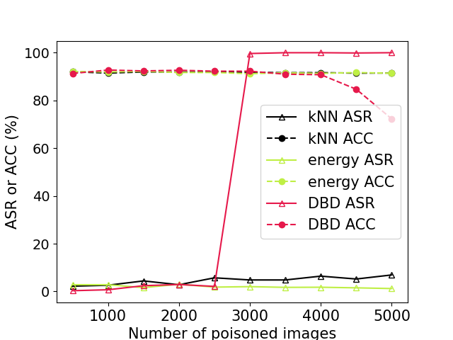
(a) Additive attack

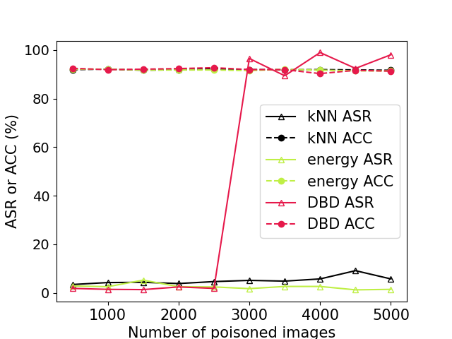
(b) blended

Fig. 2: Performance of our methods and DBD [18] for different number of attack images.

	clean	backdoor	ASR (%)	ACC (%)
baseline, without any step	100	100	98.4	94.19
AE + filtering + relabeling	22.31	5.3	3.7	51.15
SimCLR + filtering	88.95	3.2	68.9	91.94
SimCLR + relabeling	100	100	79.8	94.06
SimCLR + filtering + relabeling	88.95	3.2	4.2	92.37

Table 3: The percentage of clean (second row) and backdoor (third row) images remaining, ASR, and ACC after applying different combinations of our algorithm’s components. 1000 images were poisoned by BadNet attack.

Ablation study: In our method, three main steps are deployed for data cleaning: self-supervised contrastive training (SimCLR), data filtering, and data relabeling. Here we conduct an ablation study to understand the importance of each step. For the case without SimCLR, we still need to learn an encoder for feature embedding; an auto-encoder (AE) model is used as a substitute for SimCLR. KNN is used as the filtering method. From Tab. 3, We can see SimCLR is important for getting good embedding representations to accept most clean examples. The filtering method can reject most of the backdoor images, but if used without the relabeling, the remaining backdoor images still make the ASR high (68.9%). Also, without filtering, relabeling some backdoor samples can only slightly mitigate the ASR (to 79.8%). With the combination of SimCLR, filtering, and relabeling, our method achieves robustness against attacks even with a large number of poisoned images (shown in Fig. 2).

5 Conclusions

In this paper, we proposed a training set cleansing method against backdoor attacks. We discussed the vulnerability of supervised trained models and thus proposed to use self-supervised learned representation embedding coupled with data filtering and relabeling. Experiments show that our method is robust under different types of attacks and different attack strengths. In future, this approach could be investigated on other architectures like ViT and to mitigate non-backdoor data poisoning attacks, e.g. label flipping attacks.

Appendix A Vulnerability of supervised DNN training

Fig. 3 shows the salience map produced by GradCAM on the poisoned classifier, for an attacked test image. The salience map shows the locations in the image that the network is focusing on when making a decision. The salience map indicates that, after supervised training, when the backdoor trigger occurs, the model will focus on the backdoor trigger and ignore the other features in an image when making a decision. This indicates that the supervised trained networks build stronger “affinity” between the target class and the backdoor trigger such that the backdoor trigger will dominate the DNN’s decision-making even in the presence of clean (source class) features.

(a) attack image

(b) salient map

Fig. 3: (a): A test image with backdoor pattern. (b) the salience map produced using GradCAM on the attacked model. The test image is from Tiny-ImageNet dataset[24].

Appendix B algorithm

The algorithm of our method is given in Algorithm 1

Algorithm 1 The algorithm of our training set cleansing method.

1:Input: dataset ${\mathcal{D}}=\{(x_{i},y_{i})~{}|~{}i=1...N\}$.

2:Initialization A clean set ${\mathcal{D}}_{clean}=\{\}$; a bad set ${\mathcal{D}}_{bad}=\{\}$; and $\lambda=80$ which is used to determine the threshold of relabeling.

3:Self-supervised training: Learn an encoder $L(E(\cdot))$ based on the given dataset ${\mathcal{D}}$ using the SimCLR objective (Eq. 5).

4:for $i=1:N$ do $\triangleright$ filtering

5:     $z_{i}=L(E(x_{i}))$

6:     $c_{i}=kNN(x_{i})$ or $Energy(x_{i})$ $\triangleright$ $c_{i}$ is the class decision of the kNN or Energy method.

7:     if $c_{i}==y_{i}$ then

8:         ${\mathcal{D}}_{clean}$.insert($(x_{i},y_{i})$)

9:     else

10:         ${\mathcal{D}}_{bad}$.insert($(x_{i},y_{i})$)      

11:${\mathcal{C}}=\{Conf_{c_{i}}(x_{i})~{}|~{}x_{i}\in{\mathcal{D}}_{clean}\}$ $\triangleright$ $Conf(\cdot)$ is the confidence of kNN or Energy’s decision.

12:$T=$ percentile$({\mathcal{C}},\lambda)$ $\triangleright$ 80-th percentile of the confidences.

13:for $(x_{j},y_{j})\in{\mathcal{D}}_{bad}$ do $\triangleright$ relabeling

14:     if $Conf_{c_{j}}(x_{j})>T$  then

15:         ${\mathcal{D}}_{clean}$.insert($(x_{j},c_{j})$)      

16:Supervised training: Train a classifier $f(\cdot)$ using SupCon[20] objective on ${\mathcal{D}}_{clean}$.

17:Outputs: ${\mathcal{D}}_{clean}$; Classifier $f(\cdot)$.

Appendix C Details of attacks

In the main paper, four types of backdoor attacks are used to evaluate our method: additive attack [6], BadNet[1], blended attack[4], and WaNet[22]. Some examples of poisoned images and backdoor patterns can be found in Fig. 4.

In an additive attack, a backdoor pattern embedding function is given by $g(x,v)=[x+v]_{\rm c}$, where x represents the original image, $v$ is a small and usually imperceptible perturbation, and $[\cdot]_{\rm c}$ is a domain-dependent clipping function. The additive pattern $v$ can be either global or local. In our paper we used a global “chessboard” pattern, where one of two adjacent pixels are perturbed by 3/255 in all color channels.

BadNet uses patch replacement backdoor patterns embedded by $g(x,m,u)=(1-m)\odot x+m\odot u$ where $m$ is a $3\times 3$ mask and u is a $3\times 3$ noise patch. Both the location of the mask and the patch are randomly generated.

In the blended attack, a noise patch $u$ is blended into an image using the embedding function $g(x,\alpha,m,u)=(1-\alpha\cdot m)\odot x+\alpha\cdot m\odot u$ where $m$ is a $3\times 3$. The mask is chosen to be $3\times 3$ and the patch $u$ is a $3\times 3$ noise patch. Both the location of the mask and the patch are randomly generated. The blending rate $\alpha$ is set to 0.4 in our experiments.

WaNet is a sample-specific backdoor attack, which generates a backdoor pattern based on the image to be poisoned. In [22], the attacker is assumed to control the training process: in each training mini-batch, 10% of the images are randomly selected and poisoned. However, our defense method is applied before classifier training, so in our work, we poisoned 10% of the whole training set before training, which makes the ASR lower than that reported in the original WaNet paper when there is no defense.

“chessboard” (additive)

BadNet

blend

WaNet

Fig. 4: Example BPs considered in our main paper (top) and images with these BPs embedded (bottom). The images are from Tiny-ImageNet dataset [24].

Appendix D Experiments on other datasets

In the main paper, we showed the performance of our method on the CIFAR-10 dataset. Here we show experiments on MNIST dataset.

For MNIST, a ResNet-18 encoder is first learned using the SimCLR [19] objective for 100 epochs; then after applying data filtering and relabeling, a ResNet-18 classifier is trained using the SupCon [20] objective, on the cleansed dataset, for 100 epochs. Note that for MNIST, the pixels of the object (handwritten digits) are always white, with pixel value 255. WaNet, which will add some positive perturbation to already-white pixels (which are already at the maximum intensity), will not create an attacked image that is very different from the original image. So it will be hard for the WaNet attack to be successful on MNIST. Thus we did not include the WaNet attack in our MNIST experiment. For all the attacks, 1000 training samples are poisoned.

Tab. 4 shows that for the additive attack and blended attack, our method decreases the ASR to close to 0 with only a slight drop in ACC. The performance of our method on the BadNet attack is not as good, but the ASR is still lower than 10%.

	additive		BadNet		blend
	ASR	ACC	ASR	ACC	ASR	ACC
None	91.9	99.50	99.9	99.95	100	99.95
kNN	0.2	99.48	9.3	99.35	0.3	99.29
Energy	0	99.38	3.8	99.59	1.4	99.46

Table 4: Results on MNIST.

Appendix E Robustness to adaptive attacks

Here we evaluate the robustness of our method under an adaptive attack scenario, where the attacker has access to the whole training set and full knowledge of our defense method. If an attacker can create backdoor images that are close to the target class clean images in the embedding space, those backdoor images can survive after our filtering method; then the adaptive attack might defeat our method. However, the attacker does not control the defense process (otherwise an attacker can always be successful). Moreover, given the above assumptions of the adaptive attack, the attacker does not have access to the encoder trained using SimCLR loss in the first step of our defense method. Thus, the attacker needs to train a “surrogate” of our encoder (We assume the attacker uses the same architecture as that used by the defender.). The attacker can learn an adaptive backdoor pattern by solving the following problem:

$$u^{*}=\operatorname*{arg\,min}_{u}\frac{1}{|\mathcal{I}\backslash\mathcal{I}_{t}|}\sum_{i\in\mathcal{I}\backslash\mathcal{I}_{t}}||L(E(g(x_{i},m,u)))-\bar{z}_{t}||_{2},$$ (7)

where $g(\cdot)$ is the backdoor embedding function; here BadNet embedding is used, and $m$ is a mask fixed at top left corner of the image. $\mathcal{I}$ is the set of indices of all the images in the training set, with $\mathcal{I}_{t}$ the set of indices of images from the target class. $L(E(\cdot))$ is the “surrogate” encoder, and $\bar{z}_{t}$ is calculated as the average:

$$\bar{z}_{t}=\frac{1}{|\mathcal{I}_{t}|}\sum_{j\in\mathcal{I}_{t}}L(E(x_{j}))$$ (8)

Then by minimizing the objective function given in Eq. 7, the attacker can learn a backdoor pattern that aims to make the backdoor attacked images close to the target class images in the embedding space.

	None		kNN		Energy
	ASR	ACC	ASR	ACC	ASR	ACC
3x3 patch	96.1	93.08	9.1	91.66	7.1	92.01
7x7 patch	100	93.80	11.8	91.59	32.3	91.92
11 x 11 patch	99.9	94.49	33.4	91.86	37.9	91.82

Table 5: Adaptive attack results.

We created three poisoned CIFAR-10 datasets by varying the patch size of the BadNet pattern (3x3 patch, 7x7 patch, and 11x11 patch). The defense performance against adaptive attacks is shown in Tab. 5. The table shows that our method achieves robustness even under these adaptive attacks.

Appendix F Performance on clean dataset

Tab. 6 shows the performance comparison on a clean (unpoisoned) CIFAR-10 dataset. Our method has slightly lower ACC then DBD. Since our method will always reject some training examples even if the dataset is clean, it is reasonable in future work to first to detect if a dataset is in fact poisoned (using either existing or novel detection methods), with the filtering method applied only when a poisoned dataset is detected.

	None	DBD[18]	knn	energy
ACC	94.45	92.05	91.71	91.74

Table 6: Performance on clean CIFAR-10 dataset.

Appendix G Combining kNN and energy methods

Tab. 2 in the main paper shows the performance of our kNN based and energy based defense methods. Here we show the performance when combining the kNN and energy-based methods– an image is accepted only when it is accepted by both the kNN and energy methods; an images is relabeled only when it is relabeled by both methods and when it is relabeled to the same class. Results in Tab. 7, when compared to the results in the main paper, show that combining both methods does not lead to improved performance, which indicates that the samples accepted by both methods mostly overlap.

Add		Patch		blend		WaNet
ASR	ACC	ASR	ACC	ASR	ACC	ASR	ACC
3.3	91.23	3.5	91.43	4.2	91.29	2.2	90.44

Table 7: Results of combining kNN and energy methods.

References

- [1] T. Gu, K. Liu, B. Dolan-Gavitt, and S. Garg, “Badnets: Evaluating backdooring attacks on deep neural networks,” IEEE Access, vol. 7, pp. 47230–47244, 2019.
- [2] B. Wang, Y. Yao, S. Shan, H. Li, B. Viswanath, H. Zheng, and B.Y. Zhao, “Neural cleanse: Identifying and mitigating backdoor attacks in neural networks,” in Proc. IEEE Symposium on Security and Privacy, 2019.
- [3] Z. Xiang, D. J. Miller, H. Wang, and G. Kesidis, “Detecting scene-plausible perceptible backdoors in trained DNNs without access to the training set,” Neural Computation, vol. 33, no. 5, pp. 1329–1371, 2021.
- [4] X. Chen, C. Liu, B. Li, K. Lu, and D. Song, “Targeted backdoor attacks on deep learning systems using data poisoning,” https://arxiv.org/abs/1712.05526v1, 2017.
- [5] H. Zhong, C. Liao, A. Squicciarini, S. Zhu, and D.J. Miller, “Backdoor embedding in convolutional neural network models via invisible perturbation,” in Proc. CODASPY, 2020.
- [6] Z. Xiang, D. J. Miller, and G. Kesidis, “Detection of backdoors in trained classifiers without access to the training set,” IEEE Transactions on Neural Networks and Learning Systems, pp. 1–15, 2020.
- [7] W. Guo, L. Wang, X. Xing, M. Du, and D. Song, “TABOR: A highly accurate approach to inspecting and restoring Trojan backdoors in AI systems,” https://arxiv.org/abs/1908.01763, 2019.
- [8] Y. Liu, W. Lee, G. Tao, S. Ma, Y. Aafer, and X. Zhang, “ABS: Scanning neural networks for back-doors by artificial brain stimulation,” in Proceedings of the 2019 ACM SIGSAC Conference on Computer and Communications Security, 2019, CCS ’19, p. 1265–1282.
- [9] X. Xu, Q. Wang, H. Li, N. Borisov, C.A. Gunter, and B. Li, “Detecting AI Trojans using meta neural analysis,” in Proc. IEEE Symposium on Security and Privacy, 2021.
- [10] Hang Wang, Zhen Xiang, David J Miller, and George Kesidis, “Universal post-training backdoor detection,” arXiv preprint arXiv:2205.06900, 2022.
- [11] Y. Li, X. Lyu, N. Koren, L. Lyu, B. Li, and X. Ma, “Neural Attention Distillation: Erasing Backdoor Triggers from Deep Neural Networks,” in Proc. ICLR, 2021.
- [12] K. Liu, B. Doan-Gavitt, and S. Garg, “Fine-pruning: Defending against backdoor attacks on deep neural networks,” in Proc. RAID, 2018.
- [13] B. Chen, W. Carvalho, N. Baracaldo, H. Ludwig, B. Edwards, T. Lee, I. Molloy, and B. Srivastava, “Detecting backdoor attacks on deep neural networks by activation clustering,” http://arxiv.org/abs/1811.03728, Nov 2018.
- [14] B. Tran, J. Li, and A. Madry, “Spectral signatures in backdoor attacks,” in Proc. NIPS, 2018.
- [15] Z. Xiang, D.J. Miller, and G. Kesidis, “A benchmark study of backdoor data poisoning defenses for deep neural network classifiers and a novel defense,” in Proc. IEEE MLSP, Pittsburgh, 2019.
- [16] Z. Xiang, D. J. Miller, and G. Kesidis, “Reverse engineering imperceptible backdoor attacks on deep neural networks for detection and training set cleansing,” Computers and Security, vol. 106, 2021.
- [17] G. Schwarz, “Estimating the dimension of a model,” Annals of Stats., vol. 6, pp. 461–464, 1978.
- [18] Kunzhe Huang, Yiming Li, Baoyuan Wu, Zhan Qin, and Kui Ren, “Backdoor defense via decoupling the training process,” in International Conference on Learning Representations, 2021.
- [19] Ting Chen, Simon Kornblith, Mohammad Norouzi, and Geoffrey Hinton, “A simple framework for contrastive learning of visual representations,” in Proceedings of the 37th International Conference on Machine Learning, 2020, pp. 1597–1607.
- [20] Prannay Khosla, Piotr Teterwak, Chen Wang, Aaron Sarna, Yonglong Tian, Phillip Isola, Aaron Maschinot, Ce Liu, and Dilip Krishnan, “Supervised contrastive learning,” Advances in Neural Information Processing Systems, vol. 33, pp. 18661–18673, 2020.
- [21] A. Krizhevsky, “Learning multiple layers of features from tiny images,” University of Toronto, 05 2012.
- [22] A. Nguyen and A. Tran, “Wanet - imperceptible warping-based backdoor attack,” in International Conference on Learning Representations, 2021.
- [23] David Berthelot, Nicholas Carlini, Ian Goodfellow, Nicolas Papernot, Avital Oliver, and Colin A Raffel, “Mixmatch: A holistic approach to semi-supervised learning,” Advances in neural information processing systems, vol. 32, 2019.
- [24] J. Deng, W. Dong, R. Socher, L. Li, K. Li, and F. Li, “Imagenet: A large-scale hierarchical image database,” in 2009 IEEE Conference on Computer Vision and Pattern Recognition, 2009, pp. 248–255.