Deep Learning Based Two-dimensional Speaker Localization With Large Ad-hoc Microphone Arrays

Abstract

Deep learning based speaker localization has shown its advantage in reverberant scenarios. However, it mostly focuses on the direction-of-arrival (DOA) estimation subtask of speaker localization, where the DOA instead of the 2-dimensional (2D) coordinates is obtained only. To obtain the 2D coordinates of multiple speakers with random positions, this paper proposes a deep-learning-based 2D speaker localization method with large ad-hoc microphone arrays, where an ad-hoc microphone array is a set of randomly-distributed microphone nodes with each node set to a traditional microphone array, e.g. a linear array. Specifically, a convolutional neural network is applied to each node to get the direction-of-arrival (DOA) estimation of speech sources. Then, a triangulation and clustering method integrates the DOA estimations of the nodes for estimating the 2D positions of the speech sources. To further improve the estimation accuracy, we propose a softmax-based node selection algorithm. Experimental results with large-scale ad-hoc microphone arrays show that the proposed method achieves significantly better performance than conventional methods in both simulated and real-world environments. The softmax-based node selection further improves the performance.

I Introduction

Speaker localization aims to localize the positions of speakers with the knowledge of speech signals recorded by microphones. It finds wide applications in robotics [1], teleconferencing [2], speech separation [3], etc. It is a challenging task in adverse acoustic environments with strong reverberation and noise interference. Conventional speaker localization only requires to obtain the directions of speech sources, which is also known as the direction-of-arrival (DOA) estimation. Representative methods include the multiple signal classification (MUSIC) [4] and the steered response power with phase transform (SRP-PHAT) [5].

Recently, with the fast development of deep-learning-based speech separation and enhancement [6], deep-learning-based DOA estimation has received much attention [7, 8, 9, 10, 11, 12, 13, 14, 15]. Some methods use deep models to estimate noise-robust variables which are then used in conventional DOA estimators [8]. Some methods formulated the DOA estimation as a classification problem of azimuth classes [7]. Spatial acoustic features like generalized cross correlation [7], phase spectrograms [9], spatial pseudo-spectrum [10], and circular harmonic features [15] are usually extracted as the input of deep models. Convolutional neural networks are popular deep models for the DOA estimation [9, 10, 12, 14]. Under the above directions, many generalized problems were explored [10, 12, 11, 13]. They show improved performance over conventional approaches.

However, in many applications, obtaining a speaker’s 2-dimensional (2D) or 3-dimensional coordinate is more helpful than merely obtaining the DOA. Ad-hoc microphone arrays may be able to address the problem. An ad-hoc microphone array is a group of randomly distributed cooperative microphone nodes, each of which contains a single microphone or a traditional microphone array, like a uniform linear array. The advantages of ad-hoc microphone arrays lie in that (i) they can be easily deployed and widespread in real world by organizing online devices, and (ii) they can reduce the occurrence probability of far-field speech signal processing.

However, existing methods based on ad-hoc microphone arrays are mostly classic signal processing methods [16], which may encounter unrealistic assumptions and inaccurate parameter estimations. To our knowledge, deep-learning-based methods were studied only with distributed microphone nodes [17, 18, 19]. The work [17] trains multiple deep-learning-based nodes jointly, and predicts the 2D coordinates of speakers directly. [18] formulated the 2D localization as a classification problem of spatial grids. [19] gets the 2D coordinates by the triangulation of two distributed nodes. Although the pioneering works have shown the potential of the deep-learning-based methods, their studies were conducted with limited number of nodes (e.g. two nodes), and required additional restrictions, such as that the nodes in both training and test were fixed at the same positions [17, 18], or the spatial patterns of the nodes in both training and test should be the same [19], which do not reflect the flexibility of ad-hoc microphone arrays. As in other studies on ad-hoc arrays, e.g. [20, 21, 22, 23], an ad-hoc array that yields its advantages and superior performance over conventional fixed arrays should be able to manage massive number of nodes, as well as random positions and spatial patterns of the nodes.

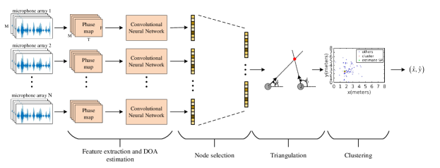
Figure 1: Diagram of the proposed 2-dimensional speaker localization method based on deep learning.

To promote the advantages of ad-hoc arrays, in this paper, we propose a deep-learning-based method with large ad-hoc microphone arrays for the 2D speaker localization. The proposed method uses convolution neural networks to estimate the DOA at each node of an ad-hoc microphone array. Then, it uses a triangulation method to obtain a roughly estimated speaker position from every two nodes. Finally, clustering is applied to get the final accurate speaker positions from the large number of roughly estimated positions. To reduce the time complexity and improve the estimation accuracy, node selection algorithms are also explored. Experimental results show that the proposed method is significantly better than conventional methods. The models trained with simulated data behave well in real-world test data.

II Proposed method

The diagram of the proposed method is shown in Fig. 1. It consists of a feature extraction module, a DOA estimation module, a node selection algorithm, and a triangulation and clustering method, which are described respectively as follows.

II-A Feature extraction and DOA estimation

Suppose a room contains an ad-hoc microphone array of $N$ nodes and $B$ speakers, where each node consists of a conventional array of $M$ microphones. In this subsection, we focus on presenting the process of the DOA estimation at a single node, given that the process is the same for all nodes.

The short-time Fourier transform (STFT) of a speech recording at the $i$th microphone of an ad-hoc node is:

$$Y_{i}(t,f)=A_{i}(t,f)e^{j\phi_{i}(t,f)},$$ (1)

where $Y_{i}(t,f)$ is the STFT at the $t$th frame and $f$th frequency bin, and $A_{i}(t,f)$ and $\phi_{i}(t,f)$ are the magnitude and phase components of the STFT respectively, $\forall i\in{1,\dots,M}$, $\forall t\in{1,\dots,T}$, and $\forall f\in{1,\dots,F}$ where $T$ is the number of the time frames of the recording and $F$ is the number of frequency bins. We group the phase spectrograms of all microphones of the node into an $M\times F\times T$ matrix, denoted as $\mathbf{\Phi}$.

The deep-learning-based DOA estimation is formulated as a classification problem of $L$ azimuth angles in the full azimuth range. Specifically, we put $\mathbf{\Phi}$ into a convolutional neural network (CNN). The reason for using CNN is that the kernel of CNN can learn the information between different microphones at every frequency bin. We denote the $t$-th time frame of $\mathbf{\Phi}$ as $\mathbf{\Phi}_{t}$, then the output of the CNN at the frame can be denoted as $p(\theta_{l}|\mathbf{\Phi}_{t})$, where $\theta_{l}$ represents the $l$-th azimuth class of the DOA. The sentence-level posterior probability of DOA can be expressed as

$$\hat{p}\left(\theta_{l}\right)=\frac{1}{T}\sum_{t=1}^{T}p\left(\theta_{l}|\mathbf{\Phi}_{t}\right).$$ (2)

If $B>1$, then the DOA estimation at the node is formulated as a multi-label classification problem [9], where the highest $B$ probabilities are the estimated DOAs of the $B$ speakers. In this paper, we take the linear array as the case of study at each node, and set $L=37$ in the $180^{\circ}$ full azimuth range.

II-B Node selection

Ad-hoc microphone array is distributed in a large acoustic scene. When a node is far from speech sources, the signal-to-noise ratio (SNR) of the signal collected by the node is low. Our studies show that (i) the SNR strongly affects the accuracy of the DOA estimation at the node, and (ii) taking all nodes whose SNRs vary in a large range in the 2D coordinate estimation of the speech sources results in a large deviation of the estimation. Therefore, we need to pick only the nodes with high SNRs into the process of the 2D coordinate estimation. As the first study of the node selection problem for the deep-learning-based speaker localization, we follow the $K$-best node selection method in [24]. To prevent training an additional deep model for the SNR estimation [24], we select the nodes according to the softmax outputs of the CNN models. Specifically, suppose the maximum of the posterior probability values produced by the CNN at the $n$-th node is $\hat{p}_{n}=\max\left(\hat{p}_{n}\left(\theta_{1}\right),\ldots,\hat{p}_{n}\left(\theta_{l}\right)\ldots,\hat{p}_{n}\left(\theta_{L}\right)\right)$, where $\hat{p}_{n}\left(\theta_{l}\right)$ is the $\hat{p}\left(\theta_{l}\right)$ of Eq. (2) at the $n$-th node. Then, we pick the $K$ nodes that yield the top $K$ largest values among $\{\hat{p}_{n}\}_{n=1}^{N}$. When the number of speakers $B>1$, we average the top $B$ largest posterior probability values at each node, and then pick the $K$ nodes as that when $B=1$.

II-C Triangulation for a rough estimation of speaker positions

We use a triangulation method to get the 2D coordinates of speakers [16]. It regards the estimated DOAs as bearing lines, and takes the cross between the bearing lines as the speaker positions. Specifically, we build a coordinate system in the room. Suppose the 2D coordinate of the $n$-th node is $\mathbf{l}_{n}=[x_{n},\ y_{n}]$, and the angle of the node with respect to the room coordinate system is $\beta_{n}$. Suppose the ground-truth 2D coordinate of the $b$-th speaker is $\mathbf{c}_{b}=[{x}_{b},\ {y}_{b}]$.

We denote the DOA estimation of the $b$-th speaker by the $n$-th node as $\hat{\theta}_{(b,n)}$. Note that, the proposed algorithm does not have to know which speaker the estimation $\hat{\theta}_{(b,n)}$ belongs to; the index $b$ is only used to remind that the proposed algorithm is suitable for multi-speaker localization. The 2D speaker localization problem is formulated as estimating $\mathbf{c}_{b}$ given $\{\mathbf{l}_{n}\}_{n=1}^{K}$, $\{\beta_{n}\}_{n=1}^{K}$, and $\{\{\hat{\theta}_{(b,n)}\}_{b=1}^{B}\}_{n=1}^{K}$. We denote $\hat{\mathbf{c}}_{b}=[\hat{x}_{b},\ \hat{y}_{b}]$ as an estimation of $\mathbf{c}_{b}$, and define $\hat{\alpha}_{(b,n)}$ as an angle between $\mathbf{l}_{n}$ and $\hat{\mathbf{c}}_{b}$ in the coordinate system:

$$\tan{\hat{\alpha}_{(b,n)}=\frac{\hat{y}_{b}-y_{n}}{\hat{x}_{b}-x_{n}}}.$$ (3)

Under the constraint that the $n$-th node is a linear array, we can obtain $\hat{\alpha}_{(b,n)}$ by:

$$\footnotesize{\hat{\alpha}_{(b,n)}=\left\{\begin{array}[]{l}\vspace{1.5ex}\beta_{n}-180^{\circ}+\hat{\theta}_{(b,n)},\mbox{ if }0^{\circ}\leq\hat{\alpha}_{(b,n)}\leq\beta_{n}\leq 180^{\circ}\\ \vspace{1.5ex}180^{\circ}-\hat{\theta}_{(b,n)}+\beta_{n},\mbox{ if }\begin{array}[]{l}\left(0^{\circ}\leq\beta_{n}\leq\hat{\alpha}_{(b,n)}\leq 180^{\circ}\right)\\ \cap\left(180^{\circ}\leq\hat{\alpha}_{(b,n)}\leq\beta_{n}+180^{\circ}\leq 360^{\circ}\right)\end{array}\\ 180^{\circ}+\hat{\theta}_{(b,n)}+\beta_{n},\mbox{ if }180^{\circ}\leq\beta_{n}+180^{\circ}\leq\hat{\alpha}_{(b,n)}\leq 360^{\circ}\end{array}\right.}$$ (4)

Note that, when other types of arrays, such as circular arrays, are used, a similar derivation can be conducted. Although we may use multiple ad-hoc nodes simultaneously to estimate the positions of the speakers, the noise and reverberation of the room makes the exact estimation of the speaker positions impossible.

In practice, the triangulation method can only get an area where a speaker may locate. To address this issue, we use two nodes for the triangulation at a time, which delivers an estimated position $[\hat{x}_{b},\hat{y}_{b}]$ as illustrated in Fig. 1. Suppose the $n_{1}$-th and $n_{2}$-th nodes are used, then the estimated position of the $b$-th speaker is obtained by:

$$\begin{array}[]{l}\hat{x}_{b}=\frac{x_{n_{1}}\tan\hat{\alpha}_{(b,n_{1})}-x_{n_{2}}\tan\hat{\alpha}_{(b,n_{2})}+y_{n_{2}}-y_{n_{1}}}{\tan\hat{\alpha}_{(b,n_{1})}-\tan\hat{\alpha}_{(b,n_{2})}},\\ \hat{y}_{b}=\frac{\tan\hat{\alpha}_{(b,n_{1})}\tan\hat{\alpha}_{(b,n_{2})}(x_{n_{1}}-x_{n_{2}})+y_{n_{2}}\tan\hat{\alpha}_{(b,n_{1})}-y_{n_{1}}\tan\hat{\alpha}_{(b,n_{2})}}{\tan\hat{\alpha}_{(b,n_{1})}-\tan\hat{\alpha}_{(b,n_{2})}}.\end{array}$$ (5)

By this way, every two nodes can get a number of roughly-estimated speaker positions. Specifically, it is well known that linear arrays cause the problem of “ghost” speakers, as illustrated in Fig. 2. Therefore, every two nodes may yield at most $B^{2}$ roughly-estimated speaker positions when there are no “ghost” speakers, and $(2B)^{2}$ positions when the “ghost” speakers exist. In other words, the triangulation does not address the multi-speaker localization problem. This difficulty can be solved by the following clustering strategy.

II-D Clustering on the rough speaker positions

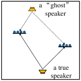
Figure 2: The “ghost” speaker problem caused by linear arrays.

To get accurate speaker positions from the rough estimations, we conduct kernel mean-shift clustering method on the rough estimations. Mean shift clustering is a nonparametric clustering algorithm. It first finds the area of the data points with the highest intensity and then gets the cluster centers by a mean shift procedure. Here we choose the Gaussian kernel mean shift clustering [25], which takes the cluster centers $\{\hat{\mathbf{c}}_{b}\}_{b=1}^{B}$ as the accurately estimated speaker positions. The advantages of the clustering strategy are that (i) a biased DOA estimation of a single node has little negative effect on the global speaker localization; (ii) the inability of the triangulation on the multi-speaker localization and “ghost” speaker problems can be easily addressed.

III Experiments on simulated data

We constructed two training sets. (i) Two-source training set: It contains 46620 training environments, each of which consists of 2 speakers speaking simultaneously; (ii) Mixed-source training set: It contains 18000 environments with 1 speaker, 36000 environments with 2 speakers, and 54000 environments with 3 speakers. Each environment randomly picks one of the 5 rooms with sizes of $6\times 6\times 2.7$m, $5\times 4\times 2.7$m, $10\times 6\times 2.7$m, $8\times 3\times 2.7$m, and $8\times 5\times 2.7$m respectively. Its reverberation time T₆₀ was selected randomly from $0.3$ to $1.0$s. The room impulse response was simulated by the image source model. The 462 training speakers of the TIMIT speech corpus, each of which uttering 10 sentences, was used as the clean speech sources. Each sound source of an environment utters one sentence. A uniform linear array (ULA) with 4 microphones was placed randomly in the room. The inter-microphone distance of the ULA was set to $8$cm. The full $180{{}^{\circ}}$ azimuth range in front of the ULA was divided evenly into $37$ azimuth angles, i.e. $L=37$, each of which corresponds to a range of $5{{}^{\circ}}$. The sound sources were placed $1$m or $2$m away from the center of the ULA in each direction. The heights of both the ULA and the sound sources were set to $1.25$m. The white noise was added by the noise generators from AudioLabs. The SNR at the ULA was uniformly sampled from $0$ to $30$dB.

We constructed 200 test environments in a room of $5\times 7\times 2.5$m with T₆₀ set to $0.4$s. For each environment, we placed 1 to 3 speakers, and an ad-hoc microphone array of 20 randomly distributed nodes, where each node is a ULA of the same configuration as that in the training data. The 168 test speakers of TIMIT were used as the clean speech sources. We added isotropic noise fields in the room with the SNR at the sound sources set to $30$dB or $40$dB.

The sampling rate of the speech recordings is 16kHz. The number of STFT points was set to 512 with a frame overlap rate of 50%. We excluded the lowest frequency sub-band of STFT, and extracted the phase spectrogram of the STFT feature from each of the four microphones of a ULA, which results in a $4\times 256$ phase map, as the input of the CNN-based DOA estimation. The CNN is a 37-class classifier, see [26] for its detailed setting. The Gaussian kernel bandwidth of the mean shift clustering was set to $0.18$m.

We created two conventional algorithms based on ad-hoc microphone arrays as the comparison baselines. They have the same structure as the proposed method, except that the CNN-based DOA estimation was replaced by conventional broadband DOA estimation methods—MUSIC and SRP-PHAT. We employed pyroomacoustics [27] to implement MUSIC and SRP-PHAT. The azimuth range of the ULAs of the baselines was divided into 180 azimuth angles, each of which corresponds to a range of 1^∘. We used mean absolute error (MAE) between the ground-truth source position $(x,y)$ and the predicted source position $(\hat{x},\hat{y})$ as the evaluation metric, which is calculated by $\mathrm{MAE}=\sqrt{(\hat{x}-x)^{2}+(\hat{y}-y)^{2}}$.

Results: We first conducted a comparison in the situation where all ad-hoc nodes were selected for the speaker localization. From the comparison results in Table I, we see that MUSIC and SRP-PHAT yield poor performance in the strongly-reverberant and noisy environment, while the proposed CNN-based method is significantly better than the baselines, no matter how the training datasets were constructed.

TABLE I: MAE (in meters) of the proposed method and the baselines on simulated data where all ad-hoc nodes are selected.

Methods	1 test speaker		2 test speakers		3 test speakers
	30dB	40dB	30dB	40dB	30dB	40dB
MUSIC	2.3360	2.3952	2.2884	2.2206	1.9406	1.9231
SRP-PHAT	2.4714	2.4415	2.2043	2.2056	1.9234	1.8665
CNN (mixed-source training)	0.2165	0.1164	0.6286	0.4152	0.8469	0.7130
CNN (two-source training)	0.0821	0.0470	0.4654	0.2034	0.7271	0.6168

To demonstrate the importance of the ad-hoc node selection scheme, we compared the all node selection method with the $K$-best node selection method where $K$ was set to $14$, $16$, and $18$ respectively. From the results in Table II, we see that the $K$-best node selection outperforms the all node selection method in three out of six test scenarios, which indicates that (i) the $K$-best node selection method is effective, and (ii) advanced node selection methods beyond the $K$-best method need further investigation.

TABLE II: MAE (in meters) of the proposed method with different numbers of selected ad-hoc nodes.

Methods	1 test speaker		2 test speakers		3 test speakers
	30dB	40dB	30dB	40dB	30dB	40dB
CNN (mixed-source training+14-best nodes)	0.1912	0.1011	0.6997	0.5030	0.9152	0.7837
CNN (mixed-source training+16-best nodes)	0.2039	0.1087	0.6888	0.4755	0.9137	0.7752
CNN (mixed-source training+18-best nodes)	0.2112	0.1384	0.6680	0.4740	0.5904	0.7479
CNN (mixed-source training+all nodes)	0.2165	0.1164	0.6286	0.4152	0.8469	0.7130
CNN (two-source training+14-best nodes)	0.0729	0.0521	0.6057	0.3319	0.7921	0.6844
CNN (two-source training+16-best nodes)	0.0950	0.0521	0.5039	0.2712	0.7540	0.6557
CNN (two-source training+18-best nodes)	0.0780	0.0467	0.4702	0.2480	0.7477	0.6443
CNN (two-source training+all nodes)	0.0821	0.0470	0.4654	0.2034	0.7271	0.6168

IV Experiments on real-world data

We recorded a real-world data set named Libri-adhoc-nodes10. It contains an office room and a conference room. Here we used the conference room as the test scenario. Fig. 3 shows the recording environment of the conference room. The size of the conference room is $4.26\times 5.16\times 3.16$m with T${}_{60}\approx 1.06$s. The room has 10 ad-hoc nodes, each of which contains a ULA that has the same configuration as the simulated data. It records the ‘test-clean’ subset of the Librispeech data replayed by a loudspeaker in the room, which contains 20 male speakers and 20 female speakers. The ad-hoc nodes and the loudspeaker have the same height of $1.3$m. The detailed description of the data and its open source will be released in another publication. To simulate the test scenarios of multiple sound sources, we summed the recordings that were generated from different loudspeaker positions.

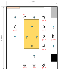
(a) Configuration 1

(b) Configuration 2

Figure 3: Recording environment and settings of the conference room of Libri-adhoc-nodes10. The red dot represents the origin of the ground coordinate system. The blue dots represent the positions of the ad-hoc nodes. The loudspeaker icons represent the positions and orientations of the speakers. Each configuration has two sub-configurations. The difference between the sub-configurations are that the directions of the ULAs at the ad-hoc nodes are different. For each sub-configuration, each position of the loudspeaker replays only one speaker. The term ‘pos’ is short for position.

Results: We evaluated the proposed method trained on the simulated data on the real-world test data. From the comparison results in Table III, we see that the proposed method significantly outperforms the two baseline methods, even if the the proposed method was trained with simulated data. The performance degradation of the proposed method on the test scenarios of 2 or more sound sources is mainly caused by the exponentially increased number of ghost speakers.

TABLE III: MAE (in meters) of the proposed method and the baselines on real-world data, where all ad-hoc nodes are selected.

Methods	1 test speaker	2 test speakers	3 test speakers
MUSIC	1.5999	1.6759	1.6987
SRP-PHAT	1.5239	1.3649	1.4278
CNN (mixed-source training)	0.4329	0.9214	1.0134
CNN (two-source training)	0.3931	0.8507	1.0371

V Conclusions

In this paper, we have developed a deep-learning-based speaker localization method with large-scale ad-hoc microphone arrays. It first applies a CNN-based DOA estimation algorithm for each ad-hoc node. Then, it selects highly-accurate nodes for the triangulation method to generate a number of roughly estimated speaker positions. Finally, it gets the accurate speaker positions by clustering the massive roughly estimated positions. We have created two comparison baselines based on MUSIC and SRP-PHAT respectively. The comparison results on both simulated data and real-world data demonstrate the effectiveness and generalization ability of the proposed method on the 2D speaker localization problem.

References

- [1] J.-M. Valin, F. Michaud, B. Hadjou, and J. Rouat, “Localization of simultaneous moving sound sources for mobile robot using a frequency-domain steered beamformer approach,” in IEEE International Conference on Robotics and Automation, 2004. Proceedings. ICRA’04. 2004, vol. 1. IEEE, 2004, pp. 1033–1038.
- [2] H. Wang and P. Chu, “Voice source localization for automatic camera pointing system in videoconferencing,” in 1997 IEEE International Conference on Acoustics, Speech, and Signal Processing, vol. 1. IEEE, 1997, pp. 187–190.
- [3] Y. Jiang, D. Wang, R. Liu, and Z. Feng, “Binaural classification for reverberant speech segregation using deep neural networks,” IEEE/ACM Transactions on Audio, Speech, and Language Processing, vol. 22, no. 12, pp. 2112–2121, 2014.
- [4] R. Schmidt, “Multiple emitter location and signal parameter estimation,” IEEE transactions on antennas and propagation, vol. 34, no. 3, pp. 276–280, 1986.
- [5] J. H. DiBiase, A high-accuracy, low-latency technique for talker localization in reverberant environments using microphone arrays. Brown University, 2000.
- [6] D. Wang and J. Chen, “Supervised speech separation based on deep learning: An overview,” IEEE/ACM Transactions on Audio, Speech, and Language Processing, vol. 26, no. 10, pp. 1702–1726, 2018.
- [7] X. Xiao, S. Zhao, X. Zhong, D. L. Jones, E. S. Chng, and H. Li, “A learning-based approach to direction of arrival estimation in noisy and reverberant environments,” in 2015 IEEE International Conference on Acoustics, Speech and Signal Processing (ICASSP). IEEE, 2015, pp. 2814–2818.
- [8] Z.-Q. Wang, X. Zhang, and D. Wang, “Robust speaker localization guided by deep learning-based time-frequency masking,” IEEE/ACM Transactions on Audio, Speech, and Language Processing, vol. 27, no. 1, pp. 178–188, 2018.
- [9] S. Chakrabarty and E. A. Habets, “Multi-speaker doa estimation using deep convolutional networks trained with noise signals,” IEEE Journal of Selected Topics in Signal Processing, vol. 13, no. 1, pp. 8–21, 2019.
- [10] T. N. T. Nguyen, W.-S. Gan, R. Ranjan, and D. L. Jones, “Robust source counting and doa estimation using spatial pseudo-spectrum and convolutional neural network,” IEEE/ACM Transactions on Audio, Speech, and Language Processing, vol. 28, pp. 2626–2637, 2020.
- [11] X. Qian, M. Madhavi, Z. Pan, J. Wang, and H. Li, “Multi-target doa estimation with an audio-visual fusion mechanism,” in ICASSP 2021-2021 IEEE International Conference on Acoustics, Speech and Signal Processing (ICASSP). IEEE, 2021, pp. 4280–4284.
- [12] W. He, P. Motlicek, and J.-M. Odobez, “Neural network adaptation and data augmentation for multi-speaker direction-of-arrival estimation,” IEEE/ACM Transactions on Audio, Speech, and Language Processing, vol. 29, pp. 1303–1317, 2021.
- [13] X. Qian, Q. Zhang, G. Guan, and W. Xue, “Deep audio-visual beamforming for speaker localization,” IEEE Signal Processing Letters, vol. 29, pp. 1132–1136, 2022.
- [14] W. Mack, J. Wechsler, and E. A. Habets, “Signal-aware direction-of-arrival estimation using attention mechanisms,” Computer Speech & Language, vol. 75, p. 101363, 2022.
- [15] K. SongGong, W. Wang, and H. Chen, “Acoustic source localization in the circular harmonic domain using deep learning architecture,” IEEE/ACM Transactions on Audio, Speech, and Language Processing, vol. 30, pp. 2475–2491, 2022.
- [16] M. Cobos, F. Antonacci, A. Alexandridis, A. Mouchtaris, and B. Lee, “A survey of sound source localization methods in wireless acoustic sensor networks,” Wireless Communications and Mobile Computing, vol. 2017, 2017.
- [17] F. Vesperini, P. Vecchiotti, E. Principi, S. Squartini, and F. Piazza, “Localizing speakers in multiple rooms by using deep neural networks,” Computer Speech & Language, vol. 49, pp. 83–106, 2018.
- [18] G. Le Moing, P. Vinayavekhin, T. Inoue, J. Vongkulbhisal, A. Munawar, R. Tachibana, and D. J. Agravante, “Learning multiple sound source 2d localization,” in 2019 IEEE 21st International Workshop on Multimedia Signal Processing (MMSP). IEEE, 2019, pp. 1–6.
- [19] S. Kindt, A. Bohlender, and N. Madhu, “2d acoustic source localisation using decentralised deep neural networks on distributed microphone arrays,” in Speech Communication; 14th ITG Conference. VDE, 2021, pp. 1–5.
- [20] J. Chen and X.-L. Zhang, “Scaling sparsemax based channel selection for speech recognition with ad-hoc microphone arrays,” in Interspeech, 2021.
- [21] C. Liang, J. Chen, S. Guan, and X.-L. Zhang, “Attention-based multi-channel speaker verification with ad-hoc microphone arrays,” in 2021 Asia-Pacific Signal and Information Processing Association Annual Summit and Conference (APSIPA ASC). IEEE, 2021, pp. 1111–1115.
- [22] Z. Yang, S. Guan, and X.-L. Zhang, “Deep ad-hoc beamforming based on speaker extraction for target-dependent speech separation,” Speech Communication, vol. 140, pp. 87–97, 2022.
- [23] C. Liang, Y. Chen, J. Yao, and X.-L. Zhang, “Multi-channel far-field speaker verification with large-scale ad-hoc microphone arrays,” in Interspeech, 2022.
- [24] X.-L. Zhang, “Deep ad-hoc beamforming,” Computer Speech & Language, vol. 68, p. 101201, 2021.
- [25] K.-L. Wu and M.-S. Yang, “Mean shift-based clustering,” Pattern Recognition, vol. 40, no. 11, pp. 3035–3052, 2007.
- [26] S. Chakrabarty and E. A. Habets, “Broadband doa estimation using convolutional neural networks trained with noise signals,” in 2017 IEEE Workshop on Applications of Signal Processing to Audio and Acoustics (WASPAA). IEEE, 2017, pp. 136–140.
- [27] R. Scheibler, E. Bezzam, and I. Dokmanić, “Pyroomacoustics: A python package for audio room simulation and array processing algorithms,” in 2018 IEEE International Conference on Acoustics, Speech and Signal Processing (ICASSP). IEEE, 2018, pp. 351–355.