$$f_{L}\left(l\right)=\cases{0}$$ l≤lmin, (1)

(2)

We refer the reader to Appendix LABEL:ap:intrinsicLengthDistribution for a derivation of this expression and a demonstration of its connection to the literature’s most common parametrisation.

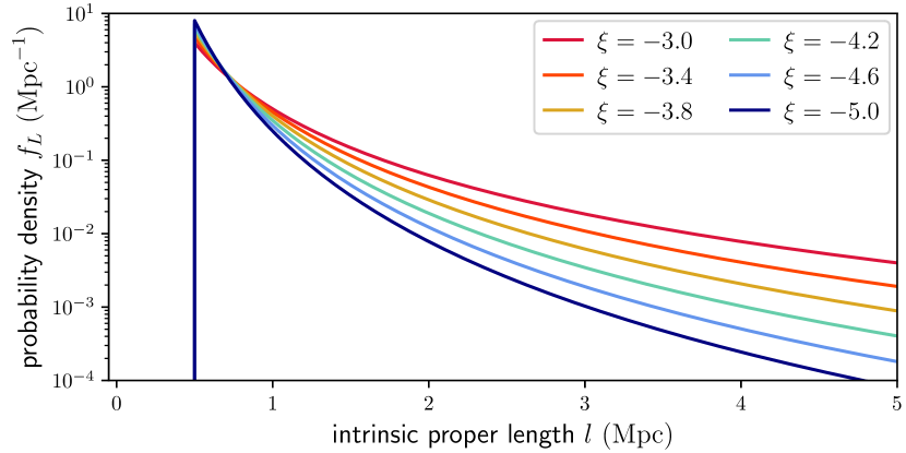
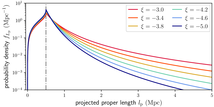
Figure 1: PDFs of radio galaxy intrinsic proper lengths $L$ and projected proper lengths $L_{\mathrm{p}}$. If the intrinsic lengths $L$ are Pareto distributed above some cut-off $l_{\mathrm{min}}$, then their projections on the sky $L_{\mathrm{p}}$ are also Pareto distributed above this cut-off. The tail indices are the same. We show the PDFs $f_{L}$ (left) and $f_{L_{\mathrm{p}}}$ (right) for $l_{\mathrm{min}}=0.5\ \mathrm{Mpc}$, $l_{\mathrm{max}}=\infty$ (see Appendix LABEL:sec:supplementaryMaterialPowerLawModel) and various tail indices $\xi$. The support of $f_{L}$ starts at $l_{\mathrm{min}}$, which is marked by the vertical grey line in the right panel.

2.2 Projected proper length

From the distribution of intrinsic lengths and the assumption of random radio galaxy orientations, we now derive the distribution of projected lengths. This distribution is more easily compared to observations, which usually lack inclination angle information.

2.2.1 Distribution for RGs

To model length and orientation, we consider a vector $\@vec{L}\in\mathbb{R}^{3}$ (of length $L\coloneqq||\@vec{L}||_{2}$) for each RG. In accordance with the IAU Solar System convention for positive poles, the unit vector $\hat{L}\in\mathbb{S}^{2}$ marks the direction from which the central Kerr black hole is seen rotating in anticlockwise direction. We define the inclination angle $\Theta$ as the angle between $\@vec{L}$ and a vector parallel to the line of sight pointing towards the observer. Observations that allow one to measure the orientation of the RG axis in 3D are time-intensive, and so usually only the RG length projected onto the plane of the sky is known.

Geometrically, we model RGs as line segments — as if they were ‘thin sticks’, with vanishing volumes — so that the projected proper length RV $L_{\mathrm{p}}$ relates to $L$ and $\Theta$ through

$$L_{\mathrm{p}}=L\sin{\Theta}.$$ (3)

We assume that $\hat{L}$ is drawn from a uniform distribution on $\mathbb{S}^{2}$, so that the PDF $f_{\Theta}:[0,\pi]\to\mathbb{R}_{\geq 0}$ becomes $f_{\Theta}\left(\theta\right)=\frac{1}{2}\sin{\theta}$. Since $L$ and $\Theta$ are independent, we find in Appendix LABEL:ap:projectedLengthDistribution that the PDF of $L_{\mathrm{p}}$, $f_{L_{\mathrm{p}}}:\mathbb{R}\to\mathbb{R}_{\geq 0}$, is where

$$I\left(a,b\right)\coloneqq\int_{1}^{\infty}\frac{\eta^{a}\ \mathrm{d}\eta}{\sqrt{\eta^{2}-b^{2}}}\text{ for }a<0,|b|<1.$$ (7)

We note that for $l_{\mathrm{p}}>l_{\mathrm{min}}$, the projected proper length has a Pareto distribution with the same tail index as the intrinsic proper length distribution. We compare $f_{L}$ and $f_{L_{\mathrm{p}}}$ in Fig. 1.

2.2.2 Distribution for giants

For giants specifically (i.e. RGs such that $L_{\mathrm{p}}>l_{\mathrm{p,GRG}}$, where $l_{\mathrm{p,GRG}}$ is some constant threshold; in this work, $l_{\mathrm{p,GRG}}\coloneqq 0.7\ \mathrm{Mpc}$), the projected proper length distribution becomes a Pareto distribution with tail index $\xi$ again: In other words, for giants, projection retains the Paretianity of lengths. A measurement of the tail index of the projected length distribution is immediately also a measurement of the tail index of the intrinsic length distribution.

The survival function, which gives the probability that a GRG has a projected proper length exceeding $l_{\mathrm{p}}$, takes on a particularly simple form:

$$\mathbb{P}\left(L_{\mathrm{p}}>l_{\mathrm{p}}\ |\ L_{\mathrm{p}}>l_{\mathrm{p,GRG}}\right)=\left(\frac{l_{\mathrm{p}}}{l_{\mathrm{p,GRG}}}\right)^{\xi+1}.$$ (10)

The mean projected proper length of giants is the expectation value of $L_{\mathrm{p}}\ |\ L_{\mathrm{p}}>l_{\mathrm{p,GRG}}$:

$$\mathbb{E}[L_{\mathrm{p}}\ |\ L_{\mathrm{p}}>l_{\mathrm{p,GRG}}]=l_{\mathrm{p,GRG}}\frac{\xi+1}{\xi+2},$$ (11)

which is only defined when $\xi<-2$. For example, when $\xi=-4$, $\mathbb{E}[L_{\mathrm{p}}\ |\ L_{\mathrm{p}}>l_{\mathrm{p,GRG}}]=\frac{3}{2}l_{\mathrm{p,GRG}}$, which becomes $1.05\ \mathrm{Mpc}$ for $l_{\mathrm{p,GRG}}\coloneqq 0.7\ \mathrm{Mpc}$ and $1.5\ \mathrm{Mpc}$ for $l_{\mathrm{p,GRG}}\coloneqq 1\ \mathrm{Mpc}$.

Appendix LABEL:ap:projectedLengthDistributionGRGs provides a derivation for all three expressions.

2.3 Deprojection factor

The deprojection factor, $D\coloneqq\frac{L}{L_{\mathrm{p}}}=\sin^{-1}{\Theta}$, quantifies how much larger intrinsic lengths are compared with projected lengths. The PDF of $D$, $f_{D}:\mathbb{R}\to\mathbb{R}_{\geq 0}$, is The mean deprojection factor $\mathbb{E}[D]=\frac{\pi}{2}$. Deprojection factors can become arbitrarily large under the current model, because projected lengths can become arbitrarily small. As discussed in Sect. LABEL:sec:movingBeyondLineSegmentProjection, this is not a very realistic set-up. In reality, an RG’s projected length is bounded from below by its lobes, which have a non-vanishing volume and thus extend along all three spatial dimensions. Upon projection, the projected length therefore cannot shrink beyond some lower limit that depends on the lobe geometry. In Appendix LABEL:ap:deprojectionFactor, we show that by enriching the conventional stick-like geometry with spherical lobes, deprojection factors indeed become bounded.

2.4 Intrinsic proper length posterior and its moments

Because an RG’s intrinsic length is more physically informative than its projected length, we ideally obtain the former. In this subsection, we quantify what a measurement $L_{\mathrm{p}}=l_{\mathrm{p}}$ already reveals about $L$.

We first note that the projected length bounds the intrinsic length from below. The intrinsic length can be much larger, however, but this is improbable for two reasons: large lengths are rarer than small lengths, although how drastic this effect is depends on $\xi$; in addition, viewing directions with large inclination angles are uncommon. The best we can do is to construct a posterior distribution for $L$ given $L_{\mathrm{p}}=l_{\mathrm{p}}$. This posterior has a concise analytic form. If $l_{\mathrm{p}}>l_{\mathrm{min}}$, which is the relevant case for giants, the distribution of $L\ |\ L_{\mathrm{p}}=l_{\mathrm{p}}$ is For $l\gg l_{\mathrm{p}}$, $f_{L|L_{\mathrm{p}}=l_{\mathrm{p}}}\left(l\right)\propto\left(\frac{l}{l_{\mathrm{p}}}\right)^{\xi-2}$: the posterior PDF tends to a power law in $l$ with index $\xi-2$. In Fig. 2, we visualise the posterior PDF for several values of $\xi$.

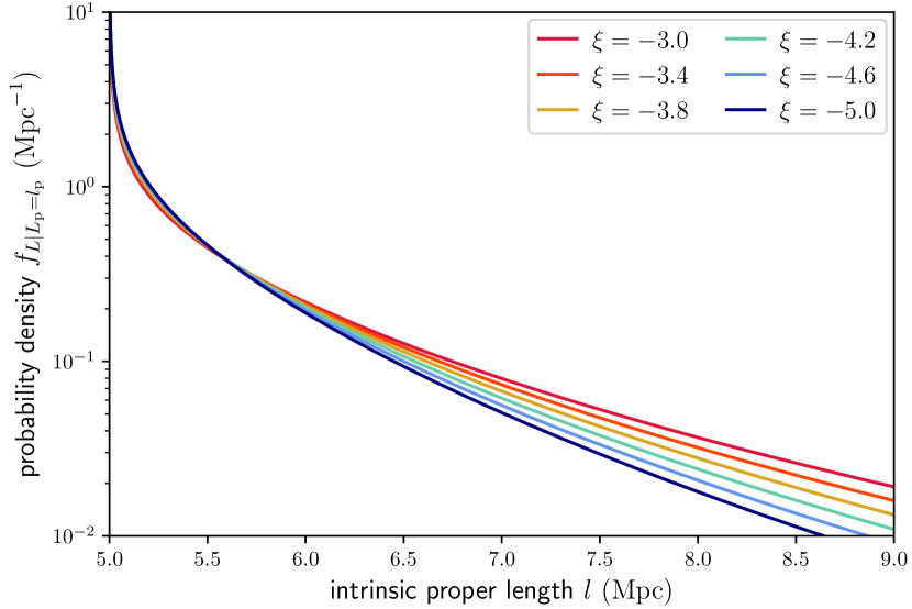
Figure 2: Posterior PDFs of intrinsic lengths for a given projected length $L\ |\ L_{\mathrm{p}}=l_{\mathrm{p}}$. If tail index $\xi$ is known, then an RG’s $l_{\mathrm{p}}$ fixes the probability distribution over its possible $l$. This distribution is strongly skewed, and the same for all $l_{\mathrm{p}}$ — save for horizontal translation and vertical scaling. We illustrate this point by showing posterior PDFs for giants with two different $l_{\mathrm{p}}$. Top: $l_{\mathrm{p}}=1\ \mathrm{Mpc}$. Bottom: $l_{\mathrm{p}}=5\ \mathrm{Mpc}$. For $\xi=-4$, the posterior mean $\mathbb{E}[L\ |\ L_{\mathrm{p}}=l_{\mathrm{p}}]=1.13\ l_{\mathrm{p}}$ and the posterior standard deviation $\sqrt{\mathbb{V}[L\ |\ L_{\mathrm{p}}=l_{\mathrm{p}}]}=0.23\ l_{\mathrm{p}}$ (see Table LABEL:tab:posteriorMoments).

Clearly, to evaluate Eq. LABEL:eq:PDFProperLengthGivenProjectedProperLength, one must choose $l_{\mathrm{p}}$ — however, the shape of the distribution is the same for all choices. We illustrate this by comparing the PDF for a comparatively small GRG ($l_{\mathrm{p}}=1.0\ \mathrm{Mpc}$; top panel) to the PDF for Alcyoneus ($l_{\mathrm{p}}=5.0\ \mathrm{Mpc}$; bottom panel).

The posterior mean is

$$\mathbb{E}\left[L\ |\ L_{\mathrm{p}}=l_{\mathrm{p}}\right]=l_{\mathrm{p}}\cdot\frac{-\xi}{2^{2\xi+3}\pi}\frac{\Gamma^{4}\left(-\frac{\xi}{2}\right)}{\Gamma^{2}\left(-\xi\right)};$$ (16)

the posterior variance is

$$\mathbb{V}\left[L\ |\ L_{\mathrm{p}}=l_{\mathrm{p}}\right]=l_{\mathrm{p}}^{2}\left(\frac{\xi}{\xi+1}-\frac{\xi^{2}}{2^{4\xi+6}\pi^{2}}\frac{\Gamma^{8}\left(-\frac{\xi}{2}\right)}{\Gamma^{4}\left(-\xi\right)}\right).$$ (17)

Both mean and standard deviation scale linearly in $l_{\mathrm{p}}$: the projection effect is a multiplicative noise source. In Table LABEL:tab:posteriorMoments, we provide explicit values for various $\xi$.

Table 1: Intrinsic proper length posterior mean and standard deviation in multiples of projected proper length $l_{\mathrm{p}}$, given for various tail indices $\xi$.

	$\mathbb{E}\left[L\ |\ L_{\mathrm{p}}=l_{\mathrm{p}}\right]\left(\xi\right)\ \ \left(l_{\mathrm{p}}\right)$	$\sqrt{\mathbb{V}\left[L\ |\ L_{\mathrm{p}}=l_{\mathrm{p}}\right]\left(\xi\right)}\ \ \left(l_{\mathrm{p}}\right)$
$\xi=-2$	$\frac{4}{\pi}\approx 1.27$	$\sqrt{2-\frac{16}{\pi^{2}}}\approx 0.62$
$\xi=-3$	$\frac{3\pi}{8}\approx 1.18$	$\sqrt{\frac{3}{2}-\frac{9\pi^{2}}{64}}\approx 0.33$
$\xi=-4$	$\frac{32}{9\pi}\approx 1.13$	$\sqrt{\frac{4}{3}-\frac{1024}{81\pi^{2}}}\approx 0.23$
$\xi=-5$	$\frac{45\pi}{128}\approx 1.10$	$\sqrt{\frac{5}{4}-\frac{2025\pi^{2}}{16384}}\approx 0.17$

Higher moments exist up to order $\lceil-\xi\rceil$; because the PDF $f_{L\ |\ L_{\mathrm{p}}=l_{\mathrm{p}}}\left(l\right)$ is strongly skewed, such moments do further specify the distribution.

It is important to note that it is formally incorrect to statistically deproject RGs by drawing samples from deprojection factor $D$ and multiplying them with some measurement $L_{\mathrm{p}}=l_{\mathrm{p}}$, or even more crudely, by multiplying the latter with $\mathbb{E}[D]$. The reason that renders such approaches invalid is that $L_{\mathrm{p}}=L\sin{\Theta}$ and $D=\sin^{-1}{\Theta}$ are not independent RVs. We refer to Appendix LABEL:ap:posterior for an explicit proof of this fact, and for derivations of this subsection’s expressions.

2.5 GRG inclination angle

Radio galaxies with jets that make a small angle with the plane of the sky are more likely to have a projected length exceeding $l_{\mathrm{p,GRG}}$ than those with jets that make a large angle with the plane of the sky. For this reason, the inclination angle distribution of giants is different from that of RGs: it is more peaked around $\theta=90\degree$. More precisely, the PDF $f_{\Theta\ |\ L_{\mathrm{p}}>l_{\mathrm{p,GRG}}}:[0,\pi]\to\mathbb{R}_{\geq 0}$ of the GRG inclination angle $\Theta\ |\ L_{\mathrm{p}}>l_{\mathrm{p,GRG}}$ has the general form

$$f_{\Theta\ |\ L_{\mathrm{p}}>l_{\mathrm{p,GRG}}}(\theta)=\frac{\left(1-F_{L}\left(\frac{l_{\mathrm{p,GRG}}}{\sin{\theta}}\right)\right)f_{\Theta}\left(\theta\right)}{1-F_{L_{\mathrm{p}}}(l_{\mathrm{p,GRG}})}.$$ (25)

Under our Pareto distribution assumption for $L$, this concretises to

$$f_{\Theta\ |\ L_{\mathrm{p}}>l_{\mathrm{p,GRG}}}(\theta)=\frac{2}{-(\xi+1)\sqrt{\pi}}\frac{\Gamma\left(-\frac{\xi}{2}+1\right)}{\Gamma\left(-\frac{\xi}{2}-\frac{1}{2}\right)}\sin^{-\xi}{\theta}.$$ (26)

We note that $f_{\Theta\ |\ L_{\mathrm{p}}>l_{\mathrm{p,GRG}}}(\theta)\propto\sin^{-\xi}{\theta}$; the factor in front serves only as a normalisation constant. The distribution is independent of the choice of $l_{\mathrm{p,GRG}}$ and depends on a single parameter: $\xi$. We visualise $f_{\Theta\ |\ L_{\mathrm{p}}>l_{\mathrm{p,GRG}}}(\theta)$ in Fig. 3.

Figure 3: PDFs of GRG inclination angles $\Theta\ |\ L_{\mathrm{p}}>l_{\mathrm{p,GRG}}$ (colours) and RG inclination angles $\Theta$ (grey). Giants more often have orientations close to the sky plane. The strength of this tendency is governed by $\xi$, with larger $\xi$ meaning more dispersion.

Appendix LABEL:ap:GRGInclinationAngle contains a brief derivation.

2.6 GRG angular length

The model predicts the distribution of GRG angular lengths in the Local Universe up to comoving distance $r_{\mathrm{max}}$. The GRG angular length RV $\Phi\ |\ L_{\mathrm{p}}>l_{\mathrm{p,GRG}}$ relates to the GRG projected proper length RV $L_{\mathrm{p}}\ |\ L_{\mathrm{p}}>l_{\mathrm{p,GRG}}$ and the comoving distance RV $R$ as

$$\Phi\ |\ L_{\mathrm{p}}>l_{\mathrm{p,GRG}}=L_{\mathrm{p}}\ |\ L_{\mathrm{p}}>l_{\mathrm{p,GRG}}\cdot\frac{1+z\left(R\right)}{R}.$$ (27)

(We note that this relation is valid only in a flat Friedmann–Lemaître–Robertson–Walker (FLRW) universe.) We also assume that the GRG number density is constant in the Local Universe. The PDF of $\Phi\ |\ L_{\mathrm{p}}>l_{\mathrm{p,GRG}}$ has useful analytic forms under two different idealisations.

In a Euclidean universe, $z(R)=0$, and the minimal GRG angular length $\phi_{\mathrm{GRG}}=\frac{l_{\mathrm{p,GRG}}}{r_{\mathrm{max}}}$. Then which is valid as long as $\xi\neq-4$.

In an expanding universe at low redshifts, the Hubble–Lemaître law $z(R)\approx\frac{R}{d_{H}}$ holds; the Hubble distance $d_{H}\coloneqq\frac{c}{H_{0}}$. In this case, Figure 4 shows GRG angular length PDFs under both idealisations.

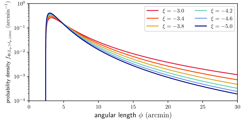
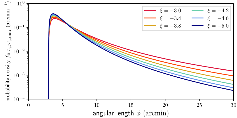
Figure 4: PDFs of GRG angular lengths $\Phi\ |\ L_{\mathrm{p}}>l_{\mathrm{p,GRG}}$. We fix $r_{\mathrm{max}}=1\ \mathrm{Gpc}$ (and $l_{\mathrm{p,GRG}}=0.7\ \mathrm{Mpc}$), and vary $\xi$. Top: Euclidean universe. Bottom: expanding universe at low redshifts.

The PDFs undergo a minor shift upon changing universe type but are otherwise similar. For most current-day applications, it will therefore be unnecessary to calculate an even more refined version of $f_{\Phi\ |\ L_{\mathrm{p}}>l_{\mathrm{p,GRG}}}(\phi)$. Appendix LABEL:ap:angularLength contains derivations and details.

2.7 Maximum likelihood estimation of the tail index

The GRG projected proper length distribution features just one parameter of physical interest: the tail index $\xi$. If observational selection effects are negligible, one can directly use maximum likelihood estimation (MLE) on GRG data to infer $\xi$. In particular, we consider a set of projected lengths $\{L_{\mathrm{p},1},...,L_{\mathrm{p},N}\}\sim L_{\mathrm{p}}\ |\ L_{\mathrm{p}}>l_{\mathrm{p,GRG}}$ from $N$ giants. Appendix LABEL:ap:MLE shows that the maximum likelihood estimate of $\xi$ is the RV $\xi_{\mathrm{MLE}}$, given by

$$\xi_{\mathrm{MLE}} =-\frac{N}{\sum_{i=1}^{N}\ln{\frac{L_{\mathrm{p},i}}{l_{\mathrm{p,GRG}}}}}-1.$$ (32)

2.8 Observed projected proper length

2.8.1 General considerations

In the preceding theory, we have ignored observational selection effects that favour some projected proper lengths over others. In practice, several such effects occur; the importance of each varies per survey and (G)RG search campaign within it. One of them is the bias against physically long RGs that the interferometer’s largest detectable angular scale can induce. As a result, the projected proper length of an observed RG might not be adequately modelled through RV $L_{\mathrm{p}}$. Instead, we must introduce a new RV $L_{\mathrm{p,obs}}$.

We define the completeness $C:\mathbb{R}_{>0}\times\mathbb{R}_{>0}\to\left[0,1\right]$ at $(l_{\mathrm{p}},z_{\mathrm{max}})$ to be the fraction of all RGs with projected proper length $l_{\mathrm{p}}$ in the cosmological volume up to $z_{\mathrm{max}}$ that is detected in a particular RG search campaign. Then, assuming that the distribution of $L_{\mathrm{p}}$ does not evolve with redshift between $z=z_{\mathrm{max}}$ and $z=0$ (i.e. $\xi$ remains constant),

$$C\left(l_{\mathrm{p}},z_{\mathrm{max}}\right)=\frac{\int_{0}^{z_{\mathrm{max}}}p_{\mathrm{obs}}\left(l_{\mathrm{p}},z\right)r^{2}\left(z\right)E^{-1}\left(z\right)\ \mathrm{d}z}{\int_{0}^{z_{\mathrm{max}}}r^{2}\left(z\right)E^{-1}\left(z\right)\ \mathrm{d}z},$$ (33)

where $p_{\mathrm{obs}}(l_{\mathrm{p}},z)$ is the probability that an RG of projected proper length $l_{\mathrm{p}}$ at cosmological redshift $z$ is detected through the campaign, and $r\left(z\right)$ is the comoving radial distance at cosmological redshift $z$. In a flat FLRW universe, the dimensionless Hubble parameter $E$ is

$$E\left(z\right)\coloneqq \frac{H\left(z\right)}{H_{0}}=\sqrt{\Omega_{\mathrm{R,0}}\left(1+z\right)^{4}+\Omega_{\mathrm{M,0}}\left(1+z\right)^{3}+\Omega_{\mathrm{\Lambda,0}}}.$$ (34)

The PDF of the observed projected proper length RV $L_{\mathrm{p,obs}}$ becomes

$$f_{L_{\mathrm{p,obs}}}\left(l_{\mathrm{p}}\right)=\frac{C\left(l_{\mathrm{p}}\right)f_{L_{\mathrm{p}}}\left(l_{\mathrm{p}}\right)}{\int_{0}^{\infty}C\left(l_{\mathrm{p}}^{\prime}\right)f_{L_{\mathrm{p}}}\left(l_{\mathrm{p}}^{\prime}\right)\ \mathrm{d}l_{\mathrm{p}}^{\prime}},$$ (35)

where we suppress the $z_{\mathrm{max}}$-dependence for succinctness. We note that multiplying $p_{\mathrm{obs}}(l_{\mathrm{p}},z)$ with an $l_{\mathrm{p}}$- and $z$-independent factor affects the completeness $C(l_{\mathrm{p}},z_{\mathrm{max}})$, but cancels in Eq. 35; $f_{L_{\mathrm{p,obs}}}$ will be independent of it. Finally, the PDF of the GRG observed projected proper length RV $L_{\mathrm{p,obs}}\ |\ L_{\mathrm{p,obs}}>l_{\mathrm{p,GRG}}$ is