Supplemental Materials for: “First constraints on light sterile neutrino oscillations from combined appearance and disappearance searches with the MicroBooNE detector”

Figure 1 shows BNB and NuMI neutrino fluxes at MicroBooNE for $\nu_{\mu}+\bar{\nu}_{\mu}$ and $\nu_{e}+\bar{\nu}_{e}$. The ratios of ($\nu_{\mu}+\bar{\nu}_{\mu}$) to ($\nu_{e}+\bar{\nu}_{e}$) are also shown in the bottom panels. The event-weighted average values of this ratio are 185.4 and 25.0 for BNB and NuMI, respectively.

\begin{overpic}[width=199.4681pt]{canv_flux_bnb.pdf} \put(455.0,-1.5){(a)} \end{overpic}

\begin{overpic}[width=199.4681pt]{canv_flux_numi.pdf} \put(455.0,-1.5){(b)} \end{overpic}

Figure 1: Intrinsic $\nu_{\mu}+\bar{\nu}_{\mu}$ and $\nu_{e}+\bar{\nu}_{e}$ fluxes as a function of true neutrino energy for (a) BNB and (b) NuMI beams at MicroBooNE in the neutrino mode. The bottom panels show the ratios of ($\nu_{\mu}+\bar{\nu}_{\mu}$) to ($\nu_{e}+\bar{\nu}_{e}$). The event-weighted average of the ratio is calculated by using the events with neutrino energy greater than 300 MeV.

Figure 2 shows the energy spectra of the seven neutrino selection channels used in the joint fit in this sterile neutrino oscillation analysis.

\begin{overpic}[width=208.13574pt]{nueCC_FC_recoEnu.pdf} \put(400.0,-35.0){(a) FC $\nu_{e}$ CC} \put(620.0,480.0){MicroBooNE} \end{overpic}

\begin{overpic}[width=208.13574pt]{nueCC_PC_recoEnu.pdf} \put(400.0,-35.0){(b) PC $\nu_{e}$ CC} \put(620.0,480.0){MicroBooNE} \end{overpic}

\begin{overpic}[width=208.13574pt]{numuCC_FC_recoEnu.pdf} \put(400.0,-35.0){(c) FC $\nu_{\mu}$ CC} \put(620.0,480.0){MicroBooNE} \end{overpic}

\begin{overpic}[width=208.13574pt]{numuCC_PC_recoEnu.pdf} \put(400.0,-35.0){(d) PC $\nu_{\mu}$ CC} \put(620.0,480.0){MicroBooNE} \end{overpic}

\begin{overpic}[width=140.92517pt]{CCpi0_FC_recoEnu.pdf} \put(400.0,-55.0){(e) FC CC$\pi^{0}$} \put(580.0,480.0){MicroBooNE} \end{overpic}

\begin{overpic}[width=140.92517pt]{CCpi0_PC_recoEnu.pdf} \put(400.0,-55.0){(f) PC CC$\pi^{0}$} \put(580.0,480.0){MicroBooNE} \end{overpic}

\begin{overpic}[width=140.92517pt]{NCpi0_recoNu.pdf} \put(400.0,-55.0){(g) NC$\pi^{0}$} \put(580.0,480.0){MicroBooNE} \end{overpic}

Figure 2: Energy spectra of the seven neutrino selection channels used in this analysis. The seven channels comprise fully contained (FC) and partially contained (PC) $\nu_{e}$ CC processes ($\nu_{e}$ CC), FC and PC $\nu_{\mu}$ CC processes without final-state $\pi^{0}$ mesons ($\nu_{\mu}$ CC), FC and PC $\nu_{\mu}$ CC processes with final-state $\pi^{0}$ mesons (CC$\pi^{0}$), and a NC channel with final-state $\pi^{0}$ mesons (NC$\pi^{0}$). Details of the selections and legend definitions can be found in Ref. [1]. The energy spectra of FC and PC $\nu_{e}$ CC channels with constraints from the other channels under the null oscillation hypothesis, and the MC prediction of the 4$\nu$ best-fit can be found in Fig. 1 in the Letter. The 4$\nu$ best fit provides approximately the same prediction as the null oscillation hypothesis for each non-$\nu_{e}$ channel.

Figure 3 shows the energy spectra of the fully contained $\nu_{e}$ CC events for different sets of oscillation parameters. The yellow and blue curves correspond to large oscillation effects, while the red curves show small oscillation effects due to the cancellation between $\nu_{e}$ disappearance and appearance when $\mathrm{sin^{2}\theta_{24}}$ approaches 0.005.

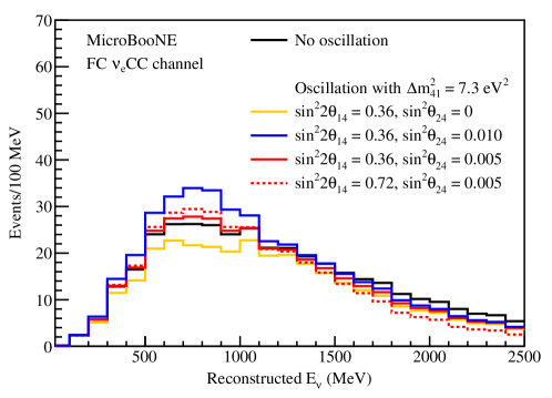
Figure 3: Energy spectra of the selected events from BNB in the fully contained (FC) $\nu_{e}$ CC channel for different sets of oscillation parameters.

Figure 4 shows the $\Delta\chi^{2}=\chi^{2}_{\mathrm{null},3\nu}-\chi^{2}_{\mathrm{min},4\nu}$ distribution obtained following the Feldman-Cousins method in comparison with the standard $\chi^{2}$ distributions with number of degrees of freedom at 2, 3 and 4.

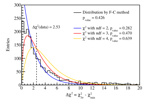
Figure 4: $\Delta\chi^{2}=\chi^{2}_{\mathrm{null},3\nu}-\chi^{2}_{\mathrm{min},4\nu}$ distribution obtained following the Feldman-Cousins (F-C) method. The figure also presents the standard $\chi^{2}$ distributions with number of degrees of freedom (ndf) at 2, 3 and 4.

Figure 5 shows MicroBooNE sensitivity and data exclusion contours at the $95\%$ $\mathrm{CL_{s}}$ in the plane of $\mathrm{\Delta m^{2}_{41}}$ and $\mathrm{sin^{2}2\theta_{\mu e}}$ or $\mathrm{sin^{2}2\theta_{ee}}$ for $\nu_{e}$ appearance-only and $\nu_{e}$ disappearance-only scenarios. The data and sensitivity differences in both scenarios originate from the overall deficit observed in the $\nu_{e}$ CC channels [1]. Figure 6 and 7 show the MicroBooNE data exclusion contours at the $95\%$ $\mathrm{CL_{s}}$ using the profiling method in the plane of $\mathrm{\Delta m^{2}_{41}}$ and $\mathrm{sin^{2}2\theta_{\mu e}}$ or $\mathrm{sin^{2}2\theta_{ee}}$ in comparison with other experimental results.

\begin{overpic}[width=208.13574pt]{canv_ue_APPonly_global_comparison.pdf} \put(500.0,-20.0){(a)} \end{overpic}

\begin{overpic}[width=208.13574pt]{canv_ee_DISonly_global_comparison.pdf} \put(500.0,-20.0){(b)} \end{overpic}

Figure 5: MicroBooNE $\mathrm{CL_{s}}$ sensitivity and data exclusion contours at the $95\%$ CL in the plane of $\mathrm{\Delta m^{2}_{41}}$ and (a) $\mathrm{sin^{2}2\theta_{\mu e}}$ or (b) $\mathrm{sin^{2}2\theta_{ee}}$. The blue solid (dashed) curve represents the MicroBooNE $95\%$ $\mathrm{CL_{s}}$ data exclusion (Asimov sensitivity) limits in the scenario of (a) $\nu_{e}$ appearance-only or (b) $\nu_{e}$ disappearance-only. In the left figure, the LSND $90\%$ and $99\%$ CL allowed regions [2] using the $\nu_{e}$ appearance-only approximation are shown as the light blue and gray shaded areas, respectively. In the right figure, the cyan shaded area represents the 2$\sigma$ allowed region of the gallium anomaly from the experimental results of GALLEX, SAGE, and BEST [3]. The 2$\sigma$ allowed region of the Neutrino-4 experiment [4] is also shown.

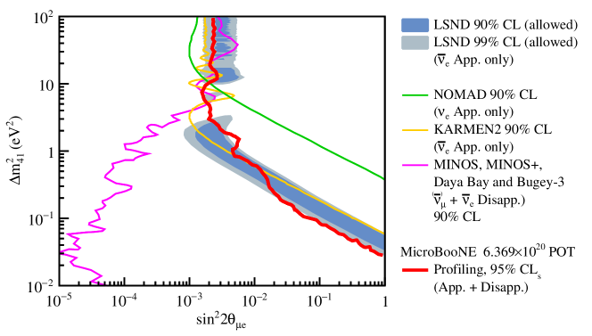
Figure 6: MicroBooNE $\mathrm{CL_{s}}$ data exclusion contour at the $95\%$ CL in the plane of $\mathrm{\Delta m^{2}_{41}}$ and $\mathrm{sin^{2}2\theta_{\mu e}}$. The figure also presents the exclusion contours at the $90\%$ CL from NOMAD [5], KARMEN2 [6], and the combined analysis of MINOS, MINOS+, Daya Bay and Bugey-3 [7]. The LSND $90\%$ and $99\%$ CL allowed regions [2] using the $\nu_{e}$ appearance-only approximation are also shown.

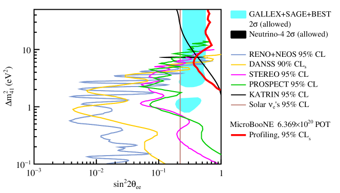
Figure 7: MicroBooNE $\mathrm{CL_{s}}$ data exclusion contour at the $95\%$ CL in the plane of $\mathrm{\Delta m^{2}_{41}}$ and $\mathrm{sin^{2}2\theta_{ee}}$. The figure also presents the exclusion contours from KATRIN [8], PROSPECT [9], STEREO [10], DANSS [11], the combined analysis of RENO and NEOS [12], and solar $\nu_{e}$’s [13]. The 2$\sigma$ allowed region of the gallium anomaly from the experimental results of GALLEX, SAGE, and BEST [3], and the 2$\sigma$ allowed region of the Neutrino-4 experiment [4] are also shown.

Figure 8 shows the MicroBooNE data exclusion contour compared with the recently updated MiniBooNE sterile neutrino oscillation result [14]. Both works take into account all possible appearance and disappearance effects within the $3+1$ oscillation framework. It is worth noting that a pure $\nu_{e}$ excess, the assumption of the $3+1$ sterile neutrino oscillation explanation to the MiniBooNE anomaly, is disfavored by the recent MicroBooNE LEE results as mentioned in the Letter. A $2\text{--}3\sigma$ tension between the MicroBooNE and MiniBooNE results can be seen in both the $\nu_{e}$ low-energy excess search [1] and the sterile neutrino oscillation search as shown in this figure.

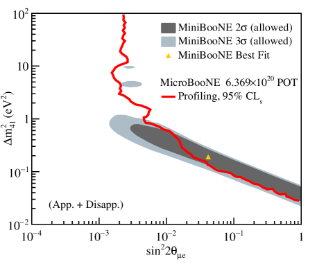
Figure 8: MicroBooNE $\mathrm{CL_{s}}$ data exclusion contour at the $95\%$ CL in the plane of $\mathrm{\Delta m^{2}_{41}}$ and $\mathrm{sin^{2}2\theta_{\mu e}}$. The MiniBooNE $2\sigma$ and $3\sigma$ CL allowed regions [14], which were calculated using the approximate test-statistic distribution from Wilks’ theorem, are also shown. Both MicroBooNE and MiniBooNE results take into account all possible appearance and disappearance effects within the $3+1$ active-to-sterile neutrino oscillation framework.

References

Abratenko et al. [2022]P. Abratenko et al. (MicroBooNE
Collaboration), Search for an
anomalous excess of inclusive charged-current interactions in the
MicroBooNE experiment using Wire-Cell reconstruction, Phys. Rev. D 105, 112005 (2022), arXiv:2110.13978 [hep-ex] .
Aguilar-Arevalo et al. [2001]A. Aguilar-Arevalo et al. (LSND
Collaboration), Evidence for
neutrino oscillations from the observation of appearance in a
beam, Phys. Rev. D 64, 112007 (2001), arXiv:hep-ex/0104049
.
Adamson et al. [2020]P. Adamson et al. (MINOS+ Collaboration,
Daya Bay Collaboration), Improved
Constraints on Sterile Neutrino Mixing from Disappearance Searches in the
MINOS, MINOS+, Daya Bay, and Bugey-3 Experiments, Phys. Rev. Lett. 125, 071801 (2020), arXiv:2002.00301 [hep-ex] .
Andriamirado et al. [2021]M. Andriamirado et al. (PROSPECT
Collaboration), Improved
short-baseline neutrino oscillation search and energy spectrum measurement
with the PROSPECT experiment at HFIR, Phys. Rev. D 103, 032001 (2021), arXiv:2006.11210 [hep-ex] .
Almazán et al. [2022]H. Almazán et al. (STEREO
Collaboration), Interpreting
Reactor Antineutrino Anomalies with STEREO data (2022) arXiv:2210.07664 [hep-ex]
.