Bayesian Optimization over Discrete and Mixed Spaces via Probabilistic Reparameterization

Abstract

Optimizing expensive-to-evaluate black-box functions of discrete (and potentially continuous) design parameters is a ubiquitous problem in scientific and engineering applications. Bayesian optimization (BO) is a popular, sample-efficient method that leverages a probabilistic surrogate model and an acquisition function (AF) to select promising designs to evaluate. However, maximizing the AF over mixed or high-cardinality discrete search spaces is challenging standard gradient-based methods cannot be used directly or evaluating the AF at every point in the search space would be computationally prohibitive. To address this issue, we propose using probabilistic reparameterization (PR). Instead of directly optimizing the AF over the search space containing discrete parameters, we instead maximize the expectation of the AF over a probability distribution defined by continuous parameters. We prove that under suitable reparameterizations, the BO policy that maximizes the probabilistic objective is the same as that which maximizes the AF, and therefore, PR enjoys the same regret bounds as the original BO policy using the underlying AF. Moreover, our approach provably converges to a stationary point of the probabilistic objective under gradient ascent using scalable, unbiased estimators of both the probabilistic objective and its gradient. Therefore, as the number of starting points and gradient steps increase, our approach will recover of a maximizer of the AF (an often-neglected requisite for commonly used BO regret bounds). We validate our approach empirically and demonstrate state-of-the-art optimization performance on a wide range of real-world applications. PR is complementary to (and benefits) recent work and naturally generalizes to settings with multiple objectives and black-box constraints.

1 Introduction

Many scientific and engineering problems involve tuning discrete and/or continuous parameters to optimize an objective function. Often, the objective function is “black-box”, meaning it has no known closed-form expression. For example, optimizing the design of an electrospun oil sorbent—a material that can be used to absorb oil in the case of a marine oil spill to mitigate ecological harm—to maximize properties such as the oil absorption capacity and mechanical strength [59] can involve tuning both discrete ordinal experimental conditions and continuous parameters controlling the composition of the material. For another example, optimizing the structural design of a welded beam can involve tuning the type of metal (categorical), the welding type (binary), and the dimensions of the different components of the beam (discrete ordinals)–resulting in a search space with over 370 million possible designs [54]. We consider the scenario where querying the objective function is expensive and sample-efficiency is crucial. In the case of designing the oil sorbent, evaluating the objective function requires manufacturing the material and measuring its properties in a laboratory, requiring significant time and resources.

Bayesian optimization (BO) is a popular technique for sample-efficient black-box optimization, due to its proven performance guarantees in many settings [52, 5] and its strong empirical performance [23, 55]. BO leverages a probabilistic surrogate model of the unknown objective(s) and an acquisition function (AF) that provides utility values for evaluating a new design to balance exploration and exploitation. Typically, the maximizer of the AF is selected as the next design to evaluate. However, maximizing the AF over mixed search spaces (i.e., those consisting of discrete and continuous parameters) or large discrete search spaces is challenging and continuous (or gradient-based) optimization routines cannot be directly applied. Theoretical performance guarantees of BO policies require that the maximizer of the AF is found and selected as the next design to evaluate on the black-box objective function [52]. When the maximizer is not found, regret properties are not guaranteed, and the performance of the BO policy may degrade.

To tackle these challenges, we propose a technique for improving AF optimization using a probabilistic reparameterization (PR) of the discrete parameters. Our main contributions are:

1. We propose a technique, probabilistic reparameterization (PR), for maximizing AFs over discrete and mixed spaces by instead optimizing a probabilistic objective (PO): the expectation of the AF over a probability distribution of discrete random variables corresponding to the discrete parameters.

2. We prove that there is an equivalence between the maximizers of the acquisition function and the the maximizers of the PO and hence, the policy that chooses designs that are best with respect to the PO enjoys the same performance guarantees as the standard BO policy.

3. We derive scalable, unbiased Monte Carlo estimators of the PO and its gradient with respect to the parameters of the introduced probability distribution. We show that stochastic gradient ascent using our gradient estimator is guaranteed to converge to a stationary point on the PO surface and will recover a global maximum of the underlying AF as the number of starting points and gradient steps increase. This is important because many BO regret bounds require maximizing the AF [52]. Although the AF is often non-convex and maximization is hard, empirically, with a modest number of starting points, PR leads to better AF optimization than alternative methods.

4. We show that PR yields state-of-the-art optimization performance on a wide variety of real-world design problems with discrete and mixed search spaces. Importantly, PR is complementary to many existing approaches such as popular multi-objective, constrained, and trust region-based approaches; in particular, PR is agnostic to the underlying probabilistic model over discrete parameters—which is not the case for many alternative methods.

2 Preliminaries

Bayesian Optimization

We consider the problem of optimizing a black-box function $f:\mathcal{X}\times\mathcal{Z}\rightarrow\mathbb{R}$ over a compact search space $\mathcal{X}\times\mathcal{Z}$, where $\mathcal{X}=\mathcal{X}^{(1)}\times\cdot\cdot\cdot\times\mathcal{X}^{(d)}$ is the domain of the $d\geq 0$ continuous parameters ($x^{(i)}\in\mathcal{X}^{(i)}$ for $i=1,...,d$) and $\mathcal{Z}=\mathcal{Z}^{(1)}\times\cdot\cdot\cdot\times\mathcal{Z}^{(d_{z})}$ is the domain of the $d_{z}\geq 1$ discrete parameters ($z^{(i)}\in\mathcal{Z}^{(i)}$ for $i=1,...,d_{z}$).

BO leverages (i) a probabilistic surrogate model—typically a Gaussian process (GP) [46]—fit to a data set $\mathcal{D}_{n}=\{\bm{x}_{i},\bm{z}_{i},y_{i}\}_{i=1}^{n}$ of designs and corresponding (potentially noisy) observations $y_{i}=f(\bm{x}_{i},\bm{z}_{i})+\epsilon_{i},\epsilon_{i}\sim\mathcal{N}(0,\sigma^{2})$, and (ii) an acquisition function $\alpha(\bm{x},\bm{z})$ that uses the surrogate model’s posterior distribution to quantify the value of evaluating a new design. Common AFs include expected improvement (EI) [32] and upper confidence bound (UCB) [52]—the latter of which enjoys no-regret guarantees in certain settings [52]. The next design to evaluate is chosen by maximizing the AF $\alpha(\bm{x},\bm{z})$ over $\mathcal{X\times Z}$. Although the black-box objective $f$ is expensive-to-evaluate, the AF is relatively cheap-to-query, and therefore, it can be optimized numerically. Gradient-based optimization routines are often used to maximize the AF over continuous domains [25].

Discrete Parameters

In its basic form, BO assumes that the inputs are continuous. However, discrete parameters such as binary, discrete ordinal, and non-ordered categorical parameters are ubiquitous in many applications. In the presence of such parameters, optimizing the AF is more difficult, as standard gradient-based approaches cannot be directly applied. Recent works have proposed various approaches including multi-armed bandits [40, 48] and local search [41] for discrete domains and interleaved discrete/continuous optimization procedures for mixed domains [15, 57]. A simple and widely-used approach across many popular BO packages [1, 53] is to one-hot encode the categorical parameters, apply a continuous relaxation when solving the optimization, and discretize (round) the resulting continuous candidates. Examples of continuous relaxations and discretization functions are listed in Table 1.

Table 1: Different parameter types, their continuous relaxations, and discretization functions.

Type	Domain	Cont. Relaxation	$\operatorname*{discretize}(\cdot)$ Function
Binary	$z\in\{0,1\}$	$z^{\prime}\in[0,1]$	$\operatorname*{round}(z^{\prime})$
Ordinal	$z\in\{0,...,C-1\}$	$z^{\prime}\in[-0.5,C-0.5)$	$\operatorname*{round}(z^{\prime})$
Categorical	$z\in\{0,...,C-1\}$	$z^{\prime}\in[0,1]^{C}$	$\operatorname*{arg\,max}_{c}z^{\prime(c)}$

Although using a continuous relaxation allows for efficient optimization using standard optimization routines in an alternate continuous domain $\mathcal{Z}^{\prime}\subset\mathbb{R}^{m}$, the AF value for an infeasible continuous value (i.e., $z^{\prime}\notin\mathcal{Z}$) does not account for the discretization that must occur before the black-box function is evaluated. Moreover, the acquisition value for an infeasible continuous value can be larger than the AF value after discretization. For an illustration of this, see Fig. 1 (middle/right). In the worst case, BO will repeatedly select the same infeasible continuous design due to its high AF value, but discretization will result in a design that has already been evaluated and has zero AF value. To mitigate this degenerate behavior and avoid the over-estimation issue, Garrido-Merchán and Hernández-Lobato [26] propose discretizing $z^{\prime}$ before evaluating the AF, but the AF is then non-differentiable with respect to the $z^{\prime}$. While this improves performance on small search spaces, the response surface has large flat regions after discretizing $z^{\prime}$, which makes it difficult to optimize the AF. The authors of [26] propose to approximate the gradients using finite differences, but, empirically, we find that this approach to be leads to sub-optimal AF optimization relative to PR.

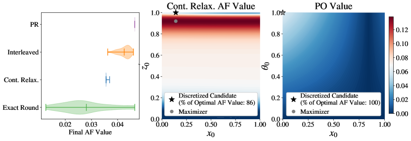
Figure 1: (Left) A comparison of AF optimization using different methods over a mixed search space shows that PR outperforms alternative methods for AF optimization and has much lower variance across replications. The violin plots show the distribution of final AF values and the mean. “Cont. Relax.” denotes optimizing a continuous relaxation of the categoricals with exact gradients. “Exact Round” refers to optimizing a continuous relaxation with approximate gradients (via finite difference), but discretizes the relaxation before evaluating the surrogate [26]. "Interleaved" alternates between one step of local search on the discrete parameters and one step of gradient ascent on the continuous parameters (used in Casmopolitan [57]). For each method, the best candidate across 20 restarts is selected (after discretization) and the acquisition value of the resulting feasible candidate is recorded. The AF is expected improvement [32]. (Middle/Right) AF values with a continuous relaxation (middle) and the PO (right) for the Branin function over a mixed domain with one continuous parameter ($x_{0}$) and one binary parameter ($z_{0})$ (see Appendix C for details on Branin). (Middle) Under a continuous relaxation, the maximizer of the AF is an infeasible point in the domain (grey circle), which results in a suboptimal AF value when rounded (black star); the resulting candidate only has 86% of the AF value of the true maximizer. The maximum AF value across the feasible search space is shown in white and the red regions indicate that the continuous relaxation overestimates the AF value since it is greater than the maximum AF value of any feasible design. (Right) The PO is maximized at the AF unique maximizer within the valid search domain. These contours show that PR avoids the overestimation issue that the naive continuous relaxation suffers from.

3 Probabilistic Reparameterization

Algorithm 1 BO with PR

1:  Input: black-box objective $f:\mathcal{X}\times\bm{Z}\rightarrow\mathbb{R}$

2:  Initialize $\mathcal{D}_{0}\leftarrow\emptyset$, $\text{GP}_{0}\leftarrow\text{GP}(\bm{0},k)$

3:  for $n=1$ to $N_{\text{iterations}}$ do

4:     $(\bm{x}_{n},\bm{\theta}_{n})\leftarrow\operatorname*{arg\,max}_{(\bm{x},\bm{\theta})\in\mathcal{X}\times\Theta}\mathbb{E}_{\bm{Z}\sim p(\bm{Z}|\bm{\theta})}[\alpha(\bm{x},\bm{Z})]$

5:     Sample $\bm{z}_{n}\sim p(\bm{Z}|\bm{\theta}_{n})$

6:     Evaluate $f(\bm{x}_{n},\bm{z}_{n})$

7:     $\mathcal{D}_{n}\leftarrow\mathcal{D}_{n-1}\cup\{(\bm{x}_{n},\bm{z}_{n},\bm{f}(\bm{x}_{n},\bm{z}_{n}))\}$

8:     Update posterior $\text{GP}_{n}$ given $\mathcal{D}_{n}$

9:  end for

We propose an alternative approach based on probabilistic reparameterization, a relaxation of the original optimization problem involving discrete parameters. Rather than directly optimizing the AF via a continuous relaxation $\bm{z}^{\prime}$ of the design $\bm{z}$, we instead reparameterize the optimization problem by introducing a discrete probability distribution $p(\bm{Z}|\bm{\theta})$ over a random variable $\bm{Z}$ with support exclusively over $\mathcal{Z}$. This distribution is parameterized by a vector of continuous parameters $\bm{\theta}$. We use $\bm{z}$ to denote the vector $(z^{(1)},...,z^{(d_{z})})$, where each element is a different (possibly vector-valued) discrete parameter. Given this reparameterization, we define the probabilistic objective (PO):

$$\mathbb{E}_{\bm{Z}\sim p(\bm{Z}|\bm{\theta})}[\alpha(\bm{x},\bm{Z})].$$ (1)

Algorithm 1 outlines BO with probabilistic reparameterization.

PR allows us to optimize $\bm{\theta}$ and $\bm{x}$ over a continuous space to maximize the PO instead of optimizing $\bm{x}$ and $\bm{z}$ to maximize $\alpha$ directly over the mixed search space $\mathcal{X}\times\mathcal{Z}$. As we will show later, maximizing the PO allows us to recover a maximizer of $\alpha$ over the space $\mathcal{X}\times\mathcal{Z}$. Choosing $p(\bm{Z}|\theta)$ to be a discrete distribution over $\mathcal{Z}$ means the realizations of $\bm{Z}$ are feasible values in $\mathcal{Z}$. Hence, the AF is only evaluated for feasible discrete designs. Since $p(\bm{Z}|\bm{\theta})$ is a discrete probability distribution, we can express $\mathbb{E}_{\bm{Z}\sim p(\bm{Z}|\bm{\theta})}[\alpha(\bm{x},\bm{Z})]$ as a linear combination where each discrete design is weighted by its probability mass:

$$\mathbb{E}_{\bm{Z}\sim p(\bm{Z}|\bm{\theta})}[\alpha(\bm{x},\bm{Z})]=\sum_{\bm{z}\in\mathcal{Z}}p(\bm{z}|\bm{\theta})\alpha(\bm{x},\bm{z}).$$ (2)

Example distributions for binary, ordinal, and categorical parameters are provided in Table 2.

Table 2: Examples of probabilistic reparameterizations for different parameter types. We denote the $(C-1)$-simplex as $\Delta^{C-1}$.

Parameter Type	Random Variable	Continuous Parameter
Binary	$Z\sim\text{Bernoulli}(\theta)$	$\theta\in[0,1]$
Ordinal	$Z=\lfloor\theta\rfloor+B,B\sim\text{Bernoulli}(\theta-\lfloor\theta\rfloor)$	$\theta\in[0,C-1]$
Categorical	$Z\sim\text{Categorical}(\theta),\theta=(\theta^{(1)},...,\theta^{(C)})$	$\theta\in\Delta^{C-1}$

Although ordinal parameters could use the same categorical distributions as the non-ordered categorical parameters, we opt for the provided proposal distribution since it uses a scalar $\theta$ (rather than a $C$-element vector) and it naturally encodes the ordering of the values. Using an independent random variable $Z^{(i)}\sim p(Z^{(i)}|\theta^{(i)})$ for each parameter $z^{(i)}$ for $i=1,...,d_{z}$ means that the probabilistic objective can be expressed as

$$\mathbb{E}_{\bm{Z}\sim p(\bm{Z}|\bm{\theta})}[\alpha(\bm{x},\bm{Z})]=\sum_{z^{(1)}\in\mathcal{Z}^{(1)}}\cdot\cdot\cdot\sum_{z^{(d_{z})}\in\mathcal{Z}^{(d_{z})}}\alpha\big{(}\bm{x},z^{(1)},...,z^{(d_{z})}\big{)}\prod_{i=1}^{d_{z}}p(z^{(i)}|\theta^{(i)}).$$ (3)

3.1 Analytic Gradients

One important benefit of PR is that the PO in (1) is differentiable with respect to $\bm{\theta}$ (and $\bm{x}$, if the gradient of $\alpha$ with respect to $\bm{x}$ exists), whereas $\alpha(\bm{x},\bm{z})$ is not differentiable with respect to $\bm{z}$. The gradients of the PO with respect to $\bm{\theta}$ and $\bm{x}$ can be obtained by differentiating Equation 2:

$$\nabla_{\bm{\theta}}\mathbb{E}_{\bm{Z}\sim p(\bm{Z}|\bm{\theta})}[\alpha(\bm{x},\bm{Z})]=\sum_{\bm{z}\in\mathcal{Z}}\alpha(\bm{x},\bm{z})\nabla_{\bm{\theta}}p(\bm{z}|\bm{\theta})$$ (4)

$$\nabla_{\bm{x}}\mathbb{E}_{\bm{Z}\sim p(\bm{Z}|\bm{\theta})}[\alpha(\bm{x},\bm{Z})]=\sum_{\bm{z}\in\mathcal{Z}}p(\bm{z}|\bm{\theta})\nabla_{\bm{x}}\alpha(\bm{x},\bm{z})$$ (5)

This enables optimizing the PO (line 4 of Algorithm 1) efficiently and effectively using gradient-based methods.

3.2 Theoretical Properties

In this section, we derive theoretical properties of PR. Proofs are provided in Appendix B. Our first result is that there is an equivalence between the maximizers of the PO and the maximizers of the AF over $\mathcal{X}\times\mathcal{Z}$.

Theorem 1 (Consistent Maximizers).

Suppose that $\alpha$ is continuous in $\bm{x}$ for every $\bm{z}\in\mathcal{Z}$. Let $\mathcal{H}^{*}$ be the maximizers of $\alpha(\bm{x},\bm{z})$: $\mathcal{H}^{*}=\{(\bm{x},\bm{z})\in\operatorname*{arg\,max}_{(\bm{x},\bm{z})\in\mathcal{X}\times\mathcal{Z}}\alpha(\bm{x},\bm{z})\}$. Let $\mathcal{J}^{*}\subseteq\mathcal{X}\times\Theta$ be the maximizers of $\mathbb{E}_{\bm{Z}\sim p(\bm{Z}|\bm{\theta})}[\alpha(\bm{x},\bm{Z})]$: $\mathcal{J}^{*}=\{(\bm{x},\bm{\theta})\in\operatorname*{arg\,max}_{(\bm{x},\bm{\theta})\in\mathcal{X}\times\Theta}\mathbb{E}_{\bm{Z}\sim p(\bm{Z}|\bm{\theta})}[\alpha(\bm{x},\bm{Z})]\}$, where $\Theta$ is the domain of $\bm{\theta}$. Let $\hat{\mathcal{H}}^{*}\subseteq\mathcal{X}\times\mathcal{Z}$ be defined as: $\hat{\mathcal{H}}^{*}=\{(\bm{x},\tilde{\bm{z}}):(\bm{x},\bm{\theta})\in\mathcal{J}^{*},\tilde{\bm{z}}\sim p(\bm{Z}|\bm{\theta})\}$. Then, $\hat{\mathcal{H}}^{*}=\mathcal{H}^{*}$.

Algorithm 1 outlines BO with probabilistic reparameterization. Importantly, Theorem 1 states that sampling from the distribution parameterized by a maximizer of the PO yields a maximizer of $\alpha$, and therefore, Algorithm 1 enjoys the performance guarantees of $\alpha(\cdot)$.

Corollary 1 (Regret Bounds).

Let $\alpha(\bm{x},\bm{z})$ be an acquisition function over a search space $\mathcal{X}\times\mathcal{Z}$ such that when $\alpha$ is applied as part of a BO strategy that strategy has bounded regret . If the conditions for the regret bounds of that BO strategy using $\alpha$ are satisfied, then Algorithm 1 using $\alpha$ enjoys the same regret bound.

Examples of BO policies with bounded regret include those based on AFs such as upper confidence bound (UCB) [52] or Thompson sampling (TS) [49] for single objective optimization, and UCB or TS with Chebyshev [43] or hypervolume [66] scalarizations in the multi-objective setting.

Although the BO policy selects a maximizer of $\alpha$ is equivalent to the BO policy in Algorithm 1, maximizing the AF over mixed or high-dimensional discrete search spaces is challenging because commonly used gradient-based methods cannot directly be applied. The key advantage of our approach is that maximizers of the AF can be identified efficiently and effectively by optimizing the PO using gradient information instead of directly optimizing the AF. We find that optimizing PR yields better results than directly optimizing $\alpha$ or other common relaxations as shown in Figure 1(Left), where we compare AF optimization methods on the mixed Rosenbrock test problem (see Appendix C for details).

4 Practical Monte Carlo Estimators

4.1 Unbiased estimators of the Probabilistic Reparameterization and its Gradient

As the number of discrete configurations ($|\mathcal{Z}|$) increases, the PO and its gradient may become computationally expensive to evaluate analytically because both require a summation of $|\mathcal{Z}|$ terms. Therefore, we propose to estimate the PO and its gradient using Monte Carlo (MC) sampling. The MC estimator of the PO is given by

$$\mathbb{E}_{\bm{Z}\sim p(\bm{Z}|\bm{\theta})}[\alpha(\bm{x},\bm{Z})]\approx\frac{1}{N}\sum_{i=1}^{N}\alpha(\bm{x},\tilde{\bm{z}}_{i}),$$ (6)

where $\tilde{\bm{z}}_{1},...,\tilde{\bm{z}}_{N}$ are samples from $p(\bm{Z}|\bm{\theta})$. This estimator is unbiased and can be computed for a large number of samples by evaluating the AF independently (or in chunks) for each input $(\bm{x},\tilde{\bm{z}}_{n})$.

MC can also be used to estimate the gradient of the PO with respect to $\bm{\theta}$. We opt for using a score function gradient estimator [35] (also known as REINFORCE [62] and the likelihood ratio estimator [27]) because it is simple, scalable, and can be computed using the acquisition values $\{\alpha(\bm{x},\tilde{\bm{z}}_{i})\}_{i=1}^{N}$ that are used in the MC estimator of the PO. Many alternative lower variance estimators (e.g. Yin et al. [65, 64]) would require many additional AF evaluations (see Mohamed et al. [39] for a review of MC gradient estimation). The score function is the gradient of the log probability with respect to the parameters of the distribution: $\nabla_{\bm{\theta}}\log p(\bm{Z}|\bm{\theta})=\frac{\nabla_{\bm{\theta}}p(\bm{Z}|\bm{\theta})}{p(\bm{Z}|\bm{\theta})}.$ Using this score function, we can express the analytic gradient as

$$\nabla_{\bm{\theta}}\mathbb{E}_{\bm{Z}\sim p(\bm{Z}|\bm{\theta})}[\alpha(\bm{x},\bm{Z})]=\sum_{\bm{z}\in\mathcal{Z}}\alpha(\bm{x},\bm{z})p(\bm{z}|\bm{\theta})\nabla_{\bm{\theta}}\log p(\bm{z}|\bm{\theta})=\mathbb{E}_{\bm{Z}\sim p(\bm{Z}|\bm{\theta})}[\alpha(\bm{x},\bm{Z})\nabla_{\bm{\theta}}\log p(\bm{Z}|\bm{\theta})].$$

The unbiased MC estimator of the gradient of the PO with respect to $\bm{\theta}$ is given by

$$\nabla_{\bm{\theta}}\mathbb{E}_{\bm{Z}\sim p(\bm{Z}|\bm{\theta})}[\alpha(\bm{x},\bm{Z})]\approx\frac{1}{N}\sum_{i=1}^{N}\alpha(\bm{x},\tilde{\bm{z}}_{i})\nabla_{\bm{\theta}}\log p(\tilde{\bm{z}}_{i}|\bm{\theta}).$$ (7)

Since the score function gradient is only defined when $p(\bm{z}|\bm{\theta})>0$, we reparameterize $\bm{\theta}$ to ensure $p(\bm{z}|\bm{\theta})>0$ for all $\bm{z}$ and $\bm{\theta}$ by using the softmax transformations provided in Table 3, which are commonly used for computational convenience and stability in probablistic reparameterization [65, 64], and the solution converges as $\tau\rightarrow 0$.

Parameter Type	Transformation ($\theta=g(\phi)$)
Binary	$\theta=\sigma((\phi-\frac{1}{2})/\tau)$
Ordinal	$\theta=\lfloor\phi\rfloor+\sigma((\phi-\lfloor\phi\rfloor-\frac{1}{2})/\tau)$
Categorical	$\theta^{(c)}=\textsc{softmax}((\bm{\phi}-0.5)/\tau)^{(c)}$

Table 3: Transformations where $\tau\in\mathbb{R}_{+}$ and $\phi,\theta\in\Theta$.

Moreover, even though $p(\bm{z}|\bm{\theta})>0$, when $p(\bm{z}|\bm{\theta})$ is small, a small number $N$ of MC samples are unlikely to produce any samples where $\tilde{\bm{z}}=\bm{z}$. Instead of optimizing $\bm{\theta}$ directly, we instead optimize $\bm{\phi}$. Since the transformations $g(\cdot)$ are differentiable with respect to $\bm{\phi}$, the gradient (and MC gradient estimator) of the PO with respect to $\bm{\phi}$ are easily obtained using the gradient of the PO with respect to $\bm{\theta}$ and a simple application the chain rule (multiplying by $\nabla_{\bm{\phi}}\bm{\theta}$).

4.2 Variance Reduction in Monte Carlo Gradient Estimation

Although the MC gradient estimator in (7) is unbiased, score function gradient estimators can suffer from high variance [39]. Therefore, we adopt a popular technique for variance reduction where the score function itself is used as a control variate, since its expectation is zero under $p(\bm{Z}|\bm{\theta})$ [39]. Score function estimators with this control variate have been shown to be among the best performing gradient estimators [39]. Moreover, this technique is simple and merely amounts to subtracting a value $\beta$ from the acquisition value in the score function estimator in Equation (7):

$$\nabla_{\bm{\theta}}\mathbb{E}_{\bm{Z}\sim p(\bm{Z}|\bm{\theta})}[\alpha(\bm{x},\bm{Z})]\approx\frac{1}{N}\sum_{i=1}^{N}[\alpha(\bm{x},\tilde{\bm{z}}_{i})-\beta]\nabla_{\bm{\theta}}\log p(\tilde{\bm{z}}_{i}|\bm{\theta}).$$ (8)

The $\beta$ is commonly known as a baseline and is often taken to be a moving average of the (acquisition) values [39]. See Appendix C for details on $\beta$.

4.3 Convergence Guarantee using Stochastic Gradient Ascent

Since the score function gradient estimator is unbiased, we can leverage previous work on convergence in probability under stochastic gradient ascent [47] to arrive at our main convergence result for acquisition optimization.

Theorem 2 (Convergence Guarantee).

Let $\alpha:\mathcal{X\times Z}\rightarrow\mathbb{R}$ be differentiable in $\bm{x}$ for every $\bm{z}\in\mathcal{Z}$. Let $(\hat{\bm{x}}_{t,m},\hat{\bm{\theta}}_{t,m})$ be the best solution after running stochastic gradient ascent for $t$ time steps on the probabilistic objective $\mathbb{E}_{\bm{Z}\sim p(\bm{Z}|\bm{\theta})}[\alpha(\bm{x},\bm{Z})]$ from $m$ starting points with its unbiased MC estimators proposed above. Let $\{a_{t}\}_{t=1}^{\infty}$ be a sequence of positive step sizes such that $0<\sum_{t=1}^{\infty}a_{t}^{2}=A<\infty$ and $\sum_{t=1}^{\infty}a_{t}=\infty$, where $a_{t}$ is the step size used in stochastic gradient ascent at time step $t$. Let $\hat{\bm{z}}_{t,m}\sim p(\bm{Z}|\hat{\bm{\theta}}_{t,m})$. Then as $t\rightarrow\infty$, $m\rightarrow\infty$, and $\tau\rightarrow 0$, $(\hat{\bm{x}}_{t,m},\hat{\bm{z}}_{t,m})\rightarrow(\bm{x}^{*},\bm{z}^{*})\in\operatorname*{arg\,max}_{(\bm{x},\bm{z})\in\mathcal{X}\times\mathcal{Z}}\alpha(\bm{x},\bm{z})$ in probability.

The significance of Theorem 2 is that optimizing the PO is guaranteed to converge in probability to a global maximizer of the AF, meaning that optimizing the PO guarantees that resulting candidate design has maximal AF value. The implication is that the intended BO policy is followed and the underlying regret bounds of the AF are recovered (provided that the other conditions of the regret bound are met). Although global convergence is only guaranteed as $m\rightarrow\infty$, we observe in Figure 1(left) that PR yields strong, stable acquisition optimization with only $m=20$ starting points, $200$ steps, and $\tau=\frac{1}{10}$ (see Appendix G for further discussion) and outperforms alternative optimization approaches.

5 Related Work

Many methods for BO over discrete and mixed search spaces have been proposed. Previous work has largely focused on (i) improving the surrogate models or (ii) improving AF optimization.

Improving models: Historically, methods leveraging tree-based surrogate models, e.g., SMAC [30] and TPE [4], have been popular for optimizing discrete or mixed search spaces. Many recent works have considered alternative surrogate models. BOCS encodes categorical parameters as binary variables and uses Bayesian linear regression with pairwise interactions [2]. COMBO uses a diffusion kernel on the graph defined by the Cartesian product of discrete parameters [41]. MerCBO similarly exploits the combinatorial graph, but with Mercer features and Thompson sampling [16]. HyBO extends the diffusion kernels to mixed continuous-discrete spaces [15]. However, these methods scale poorly with respect to the number of data points and parameters. Moreover, of the methods listed above, only HyBO supports continuous parameters without restricting them to a discrete set. HyBO enjoys a universal function approximation property, but relies on summing over all possible orders of interactions between base kernels for each parameter which results in exponential complexity with respect to the number of parameters and limits its applicability to low-dimensional problems. Moreover, the computational issues of such approaches make it difficult to apply them to multi-objective and constrained optimization. Gryffin [29] uses kernel density estimation, but is limited to categorical search spaces. MiVaBO uses a linear combination of basis functions (e.g. pseudo Boolean features [7] for discrete parameters) with interaction terms[13]. MVRSM [6] uses ReLU-based surrogates for computational efficiency, but is limited by the expressiveness of these models.

Optimizing acquisition functions: As discussed previously, Garrido-Merchán and Hernández-Lobato [26] propose using continuous relaxation and discretize the inputs before evaluating the AF. However, the resulting AF after discretization is piece-wise-flat along slices of the continuous relaxation of the discrete parameters and therefore is difficult to optimize. CoCaBO [48] samples discrete parameters using a multi-armed bandit and optimizes the continuous parameters conditional upon the sampled discrete parameters. However, CoCaBO’s performance degrades as number of discrete configurations increases. Casmopolitan [57] uses local trust regions combined with an interleaved AF optimization strategy that alternates between local search steps on the discrete parameters and gradient ascent for the continuous parameters. Furthermore, both CoCaBO and Casmopolitan do not inherently exploit ordinal structure.

Probabilistic reparameterization: PR has been considered for optimizing discrete parameters in other domains such as reinforcement learning [62] and sparse regression [65]. However, PR has not been leveraged for BO. Although the reparameterization trick used by Wilson et al. [63] is in a similar vein to PR, Wilson et al. [63] reparameterize an existing multivariate normal random variable in terms of standard normal random variables and then use sample-path gradient estimators. In contrast, our approach introduces a new probabilistic formulation using discrete probability distributions and uses likelihood-ratio-based gradient estimators since sample-path gradients cannot be computed through discrete sampling.

Alternative methods for propagating gradients: Alternative methods for propagating gradients through discrete structures have been considered in the deep learning community (among others). One approach is to use approximate discrete Concrete distributions [37, 31], which admit sample-path gradients. However, samples from Concrete distributions are not discrete and approximation error can result in pathologies similar to evaluating the AF using continuous relaxation. Moreover, approximately discrete samples prohibit using surrogate models that require discrete inputs (without discretizing the samples)—e.g., GPs with Hamming distance kernels [48]. Another approach for gradient propagation in the deep learning community is to use straight-through gradient estimators (STE) [3], where the gradient of the discretization function with respect to its input is estimated using, for example, an identity function. This approach works well empirically in some cases, these estimators are not well-grounded theoretically. Nevertheless, we discuss and evaluate using STE for AF optimization in Appendix H.

6 Experiments

In this section, we provide an empirical evaluation of PR on a suite of synthetic problems and real world applications. For PR, we use stochastic mini-batches of $N=128$ MC samples in our experiments and demonstrate that PR is robust with respect to the number of MC samples (and compare against analytic PR, where computationally feasible) in Appendix F. We optimize PR using Adam [34] with an initial learning rate of $\frac{1}{40}$. We show that PR Adam is generally robust to the choice of learning rate (more so than vanilla stochastic gradient ascent) in the sensitivity analysis in Figure 21 in Appendix M. We compare PR against two alternative acquisition optimization strategies: using a continuous relaxation (Cont. Relax.) and using exact discretization with approximate gradients (Exact Round) [26]. These approaches optimize the acquisition function with L-BFGS-B with exact and approximate gradients, respectively. In addition, we compare against two state-of-the-art methods for discrete/mixed BO: a modified version of Casmopolitan [57] that additionally supports ordinal variables introduced in Wan et al. [58] and HyBO [15], both of which are shown to outperform the other related works discussed in Section 5. In addition, we showcase how PR is complementary to existing methods such as trust region methods [22]. We demonstrate this by using PR with a trust region for the continuous and discrete ordinal parameters and optimize PR within this trust region. In Appendix H, we provide comparison of TR methods with alterative optimizers and find that PR is the best optimizer when using TRs on 6 of the 7 benchmark problems. See Appendix C for additional discussion of PR + TR. For PR, Exact Round, and PR + TR we use the sum of a product kernel and a sum kernel of a categorical kernel [48] for the categorical parameters and Matérn-5/2 kernel for all other parameters. Alternative kernels over different representations of categorical parameters such as one-hot encoded vectors, latent embeddings [67], and known embeddings (e.g. using fingerprint-based reaction encodings for categorical parameters in chemical reaction optimization [51]) are evaluated in Appendix J.

Cont. Relax., Exact Round, PR, and PR + TR use expected improvement [32, 24] for single objective (constrained problems) and expected hypervolume improvement [20] for the multi-objective oil sorbent problem (where exact gradients with respect to continuous parameters are computed using auto-differentiation [8]). We report the mean for each method $\pm$ 2 standard errors across 20 replications. Performance is evaluated in terms of regret (feasible regret for constrained problems and hypervolume regret for multi-objective problems). Casmopolitan and HyBO are not run on Welded Beam and Oil Sorbent as they do not support constrained and multi-objective optimization. We also leave the multi-objective extension of PR+TR to future work because it would add additional complexity [11]. For HyBO, we only run 60 BO iterations on SVM due to the large wall time (see Figure 3) and only report partial results on Cellular Network due to a singular covariance matrix error. See Appendix C for details on the experiment setup, regret metrics, benchmark problems, and methodological details. We leverage existing open source implementations of Casmopolitan and HyBO (see Appendix C for links), and the implementations of all of other methods are available at https://github.com/facebookresearch/bo_pr.

6.1 Synthetic Problems

We evaluate all methods on 3 synthetic problems. Ackley is a 13-dimensional function with 10 binary and 3 continuous parameters (a modified version of the problem in Bliek et al. [6]). Mixed Int F1 is a 16-dimensional variant of the F1 function from Tušar et al. [56] with 2 binary, 6 discrete ordinal parameters, and 8 continuous parameters. The discrete ordinal parameters have following cardinalities: 2 parameters with 3 values, 2 with 5 values, and 2 with 7 values. Rosenbrock is a 10-dimensional Rosenbrock function with 6 discrete ordinal parameters with 4 values each and 4 continuous parameters.

6.2 Real World Problems

We consider 5 real world applications including a problem with 5 black-box outcome constraints and a 3-objective problem (see Appendix D for details on constrained and multi-objective BO).

Welded Beam Optimizing the design of a welded steel beam is a classical engineering optimization. In this problem, the goal is to minimize manufacturing cost subject to 5 black-box constraints on structural properties of the beam (including shear stress, bending stress, and buckling load) by tuning 6 parameters: the welding configuration (binary), the metal material type (categorical with 4 options), and 4 ordinal parameters controlling the dimensions of the beam [54].

SVM Feature Selection This problem involves jointly performing feature selection and hyperparameter optimization for a Support Vector Machine (SVM) trained on the CTSlice UCI data set [18, 36]. The design space for this problem involves 50 binary parameters controlling whether a particular feature is included or not, and 3 continuous hyperparameters of the SVM.

Cellular Network Optimization In this 30-dimensional problem, the goal is to tune the tilt (ordinal with 6 values) and transmission power (continuous) for a set of 15 antennas [50] to maximize a coverage quality metric that is a function of signal power and interference [38] over a geographic region of interest. We use the simulator from Dreifuerst et al. [17].

Direct Arylation Chemical Synthesis Palladium-catalysed direct arylation has generated significant interest in the pharamceutical development sector[12]. In this problem, the goal is maximize yield for a direct arylation chemical reaction by tuning 3 categorical parameters corresponding to the choice of solvent, base, and ligand, as well 2 continuous parameters controlling the temperature and concentration. We fit a surrogate model to the direct arylation dataset from Shields et al. [51] in order to facilitate continuous optimization of temperature and concentration. In Appendix J, we demonstrate that PR can leverage a kernel over fingerprint-based reaction encodings computed via density functional theory (DFT) for the categorical parameters [51].

Electrospun Oil Sorbent Marine oil spills can cause ecological catastrophe. One avenue for mitigating environmental harm is to design and deploy absorbent materials to capture the spilled oil. In this problem, we tune 5 ordinal parameters (3 parameters with 5 values and 2 with 4 values) and 2 continuous parameters controlling the composition and manufacturing conditions for an electrospun oil sorbent material to maximize 3 competing objectives: the oil absorbing capacity, the mechanical strength, and the water contact angle [59].

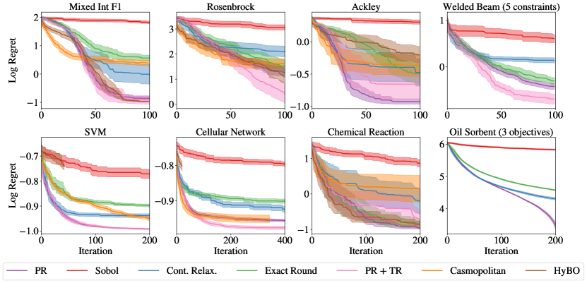
Figure 2: PR (or PR + TR) consistently outperforms alternatives with respect to log regret.

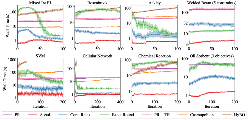
Figure 3: Wall time for candidate generation at each BO iteration in seconds. Cont. Relax., Exact Round, PR, and PR + TR are run on a single Tesla V100-SXM2-16GB GPU and other methods are run on an Intel Xeon Gold 6252N CPU.

6.3 Results

We find PR consistently delivers strong empirical performance as shown in Figure 2. On all benchmark problems, PR (or PR + TR) outperforms all baseline methods (except for Mixed Int F1, where HyBO performs comparably). Figure 3 shows the wall time for candidate generation over the number of BO iterations. Although PR is computationally intensive, the computation is embarrassingly parallel and therefore exploiting GPU acceleration yields competitive wall times. Importantly, PR’s wall time scales well with the number of observations and design parameters, unlike HyBO which scales poorly with both. However, the complexity of PR scales additively in the number of GPs being used (e.g. outcomes being modeled), assuming they are evaluated sequentially. Hence, in multi-objective or constrained settings, PR incurs a high cost in terms of wall time. However, empirically PR achieves better optimization performance on constrained and multi-objective problems relative to Cont. Relax. and Exact Round. We note that Casmopolitan does not support multi-objective BO or constrained BO, and although HyBO could be used in those settings, it would be impractically slow because 1) its wall time would scale linearly with the number of modeled outcomes (using independent GPs) and 2) its diffusion kernel is non-differentiable, which would make optimizing hypervolume-based AFs slow [8, 9].

7 Discussion

The performance and regret properties of BO depend critically on properly maximizing the AF. For problems with discrete features, exhaustively trying all possible combinations of discrete values quickly becomes infeasible as the number of combinations grows. Alternatives such as trying a subset of the possible combinations or resorting to continuous relaxations often leads to a failure to effectively optimize the AF which may result in sub-optimal BO performance. As an alternative, we propose using PR to better optimize the AF, and we demonstrate that PR achieves strong performance on a large number of real-world problems. Our approach is complementary to many other BO extensions, and combines seamlessly with, for example, trust region-based BO and specialized kernels for discrete parameters. One limitation of PR is that it requires computationally-demanding MC integration. However, given that the computation in PR is embarrassingly parallel, it motivates for future research on optimizing AFs on distributed hardware.

Checklist

1. For all authors…

   1. Do the main claims made in the abstract and introduction accurately reflect the paper’s contributions and scope? [Yes]

   2. Did you describe the limitations of your work? [Yes]

   3. Did you discuss any potential negative societal impacts of your work? [Yes] See Appendix A.

   4. Have you read the ethics review guidelines and ensured that your paper conforms to them? [Yes]

2. If you are including theoretical results…

   1. Did you state the full set of assumptions of all theoretical results? [Yes]

   2. Did you include complete proofs of all theoretical results? [Yes]

3. If you ran experiments…

   1. Did you include the code, data, and instructions needed to reproduce the main experimental results (either in the supplemental material or as a URL)? [Yes]

   2. Did you specify all the training details (e.g., data splits, hyperparameters, how they were chosen)? [Yes]

   3. Did you report error bars (e.g., with respect to the random seed after running experiments multiple times)? [Yes]

   4. Did you include the total amount of compute and the type of resources used (e.g., type of GPUs, internal cluster, or cloud provider)? [Yes] See Appendix C.

4. If you are using existing assets (e.g., code, data, models) or curating/releasing new assets…

   1. If your work uses existing assets, did you cite the creators? [Yes]

   2. Did you mention the license of the assets? [Yes] See Appendix C.

   3. Did you include any new assets either in the supplemental material or as a URL? [No]

   4. Did you discuss whether and how consent was obtained from people whose data you’re using/curating? [N/A]

   5. Did you discuss whether the data you are using/curating contains personally identifiable information or offensive content? [N/A]

5. If you used crowdsourcing or conducted research with human subjects…

   1. Did you include the full text of instructions given to participants and screenshots, if applicable? [N/A]

   2. Did you describe any potential participant risks, with links to Institutional Review Board (IRB) approvals, if applicable? [N/A]

   3. Did you include the estimated hourly wage paid to participants and the total amount spent on participant compensation? [N/A]

 
Appendix to:
Bayesian Optimization over Discrete and Mixed Spaces via Probabilistic Reparameterization
 

Appendix A Potential Societal Impacts

Our work advances Bayesian optimization, a generic class of methods for optimization of expensive, difficult-to-optimize black-box problems. With this paper in particular, we improve the performance of Bayesian optimization on problems with mixed types of inputs. Given the ubiquity of such problems in many practical applications, we believe that our method could lead to positive broader impacts by solving these problems better and more efficiently while reducing the costs incurred for solving them. Concrete and high-stake examples where our method could be potentially applied (some of which have been already demonstrated by the benchmark problems considered in the paper) include but are not limited to applications in communications, chemical synthesis, drug discovery, engineering optimization, tuning of recommender systems, and automation of machine learning systems. On the flip side, while the method proposed is ethically neutral, there is potential of misuse given that the exact objective of optimization is ultimately decided by the end users; we believe that practitioners and researchers should be aware of such possibility and aim to mitigate any potential negative impacts to the furthest extent.

Appendix B Theoretical Results and Proofs

B.1 Results

Let $\mathcal{P}_{\mathcal{Z}}^{(i)}:=\mathcal{P}(\mathcal{Z}^{(i)})$ denote the set of probability measures on $\mathcal{Z}^{(i)}$ for each $i=1,...,d_{z}$, and let $\mathcal{P}_{\mathcal{Z}}:=\prod_{i=1}^{d_{z}}\mathcal{P}_{\mathcal{Z}}^{(i)}$. For any $\alpha:\mathcal{X}\times\mathcal{Z}\rightarrow\mathbb{R}$, define $\tilde{\alpha}:\mathcal{X}\times\mathcal{P}\rightarrow\mathbb{R}$ as

$$\tilde{\alpha}(\bm{x},p)=\int_{\mathcal{Z}}\alpha(\bm{x},\bm{z})dp(\bm{z})=\sum_{\bm{z}\in\mathcal{Z}}\alpha(\bm{x},\bm{z})p(\{\bm{z}\}).$$ (9)

Let $\Theta$ be a compact metric space, and consider the set of functionals $\Phi=\{\varphi~{}s.t.~{}\varphi:\Theta\rightarrow\mathcal{P}_{\mathcal{Z}}\}$. Let

$$\hat{\alpha}(\bm{x},\bm{\theta}):=\tilde{\alpha}(\bm{x},\bm{\varphi}(\bm{\theta}))=\int_{\mathcal{Z}}\alpha(\bm{x},\bm{z})dp_{\varphi(\bm{\theta})}(\bm{z})=\sum_{\bm{z}\in\mathcal{Z}}\alpha(\bm{x},\bm{z})p_{\varphi(\bm{\theta})}(\{\bm{z}\})$$ (10)

Since $\mathcal{Z}$ is finite, each element of $\varphi\in\Phi$ can be expressed as a mapping from $\Theta$ to $\mathbb{R}^{|\mathcal{Z}|}$. Namely, each $\varphi(\bm{\theta})$ corresponds to a vector with $|\mathcal{Z}|$ elements containing the probability mass for each element of $\mathcal{Z}$ under $p_{\varphi}(\bm{\theta})$. Thus $(\mathcal{P}_{\mathcal{Z}},\|\cdot\|)$ is a metric space under any norm $\|\cdot\|$ on $\mathbb{R}^{|Z|}$. Let $\alpha^{*}:=\max_{(\bm{x},\bm{z})\in(\mathcal{X}\times\mathcal{Z})}\alpha(\bm{x},\bm{z})$ and let $\mathcal{H}^{*}:=\operatorname*{arg\,max}_{(\bm{x},\bm{z})\in(\mathcal{X}\times\mathcal{Z})}\alpha(\bm{x},\bm{z})$ denote the set of maximizers of $\alpha$.

Lemma 1.

Suppose $\alpha$ is continuous in $\bm{x}$ for every $\bm{z}\in\mathcal{Z}$ and that $\varphi:\Theta\mapsto(\mathcal{P}_{\mathcal{Z}},\|\cdot\|)$ is continuous with $\varphi(\Theta)=\mathcal{P}_{\mathcal{Z}}$. Let $\mathcal{J}^{*}:=\operatorname*{arg\,max}_{(\bm{x},\bm{\theta})\in\mathcal{X}\times\Theta}\hat{\alpha}(\bm{x},\bm{\theta})$. Then for any $(\bm{x}^{*},\bm{\theta}^{*})\in\mathcal{J}^{*}$, it holds that $(\bm{x}^{*},\bm{z})\in\mathcal{H}^{*}$ for all $z\in\mathrm{supp}\,p_{\varphi(\bm{\theta}^{*})}$.

Proof.

First, note that $\hat{\alpha}:\mathcal{X}\times\Theta\rightarrow\mathbb{R}$ is continuous (using that $\varphi$ is continuous and $\alpha$ is bounded). Since both $\mathcal{X}$ and $\Theta$ are compact $\hat{\alpha}$ attains its maximum, i.e., $\mathcal{J}^{*}$ exists. Let $(\bm{x}^{*},\bm{\theta}^{*})\in\mathcal{J}^{*}$. Clearly, there exists $\bm{z}^{*}\in\operatorname*{arg\,max}_{\bm{z}\in\mathcal{Z}}\alpha(\bm{x}^{*},\bm{z})$ such that $\alpha(\bm{x}^{*},\bm{z}^{*})=\alpha^{*}$. Suppose there exists $\bm{z}^{\prime}\in\mathrm{supp}\,p_{\varphi(\bm{\theta}^{*})}$ such that $(\bm{x}^{*},\bm{z}^{\prime})\notin\mathcal{H}^{*}$. Then $\alpha(\bm{x}^{*},\bm{z}^{\prime})<\alpha^{*}$ and, since $\mathcal{Z}$ is finite, $p_{\varphi(\bm{\theta}^{*})}(\{\bm{z}^{\prime}\})>0$. Consider the probability measure $p^{\prime}$ given by

$$p^{\prime}(\{\bm{z}\})=\Biggl{\{}\begin{array}[]{ll}0&\text{ if }\bm{z}=\bm{z}^{\prime}\\ p_{\varphi(\bm{\theta}^{*})}(\{\bm{z}^{*}\})+p_{\varphi(\bm{\theta}^{*})}(\{\bm{z}^{\prime}\})&\text{ if }\bm{z}=\bm{z}^{*}\\ p_{\varphi(\bm{\theta}^{*})}(\{\bm{z}\})&\text{ otherwise}\end{array}$$

Then

$$\tilde{\alpha}(\bm{x}^{*},p^{\prime})-\hat{\alpha}(\bm{x}^{*},\bm{\theta}^{*}) =\sum_{\bm{z}\in\mathcal{Z}}\alpha(\bm{x}^{*},z)p^{\prime}(\{\bm{z}\})-\hat{\alpha}(\bm{x}^{*},\bm{\theta}^{*})$$

$$=\sum_{\bm{z}\in\mathcal{Z}}\alpha(\bm{x}^{*},\bm{z})p_{\varphi(\bm{\theta}^{*})}(\{\bm{z}\})+p_{\varphi(\bm{\theta}^{*})}(\{\bm{z}^{\prime}\})(\alpha(\bm{x}^{*},\bm{z}^{*})-\alpha(\bm{x}^{*},\bm{z}^{\prime}))$$

$$~{}~{}~{}~{}~{}~{}~{}~{}~{}~{}-\hat{\alpha}(\bm{x}^{*},\bm{\theta}^{*})$$

$$=p_{\varphi(\bm{\theta}^{*})}(\{\bm{z}^{\prime}\})(\alpha(\bm{x}^{*},\bm{z}^{*})-\alpha(\bm{x}^{*},\bm{z}^{\prime}))$$

$$>0$$

Now $p^{\prime}\in\mathcal{P}_{\mathcal{Z}}$, and so $p^{\prime}=\varphi(\bm{\theta}^{\prime})$ for some $\bm{\theta}^{\prime}\in\Theta$. But then $\hat{\alpha}(\bm{x}^{*},\bm{\theta}^{\prime})>\hat{\alpha}(\bm{x}^{*},\bm{\theta}^{*})$. This is a contradiction. ∎

Corollary 2.

Suppose the optimizer of $g$ is unique, i.e., that $\mathcal{H}^{*}=\{(\bm{x}^{*},\bm{z}^{*})\}$ is a singleton. Then the optimizer of $\hat{\alpha}$ is also unique and $\mathcal{J}^{*}=\{(\bm{x}^{*},\bm{\theta}^{*})\}$, with $p_{\varphi(\bm{\theta}^{*})}(\{\bm{z}^{*}\})=1$.

Corollary 3.

Consider the following mappings:

• Binary: $\varphi:[0,1]\rightarrow\mathcal{P}_{\{0,1\}}$ with $p_{\varphi(\theta)}(\{1\})=\theta$ and $p_{\varphi(\theta)}(\{0\})=1-\theta$.

• Ordinal: $\varphi:[0,C-1]\rightarrow\mathcal{P}_{\{0,1,\dotsc,C\}}$ with $p_{\varphi(\theta)}(\{i\})=(1-|i-\theta|)\,\mathbf{1}\{|i-\theta|\leq 1\}$ for $i=1,\dotsc,C$.

• Categorical: $\varphi:[0,1]^{C}\rightarrow\mathcal{P}_{\{0,1,\dotsc,C\}}$ with $p_{\varphi(\theta)}(\{i\})=\frac{\theta_{i}}{\sum_{i=1}^{C}\theta_{i}}$.

These mappings satisfy the conditions for Lemma 1. In the setting with multiple discrete parameters where the above mappings are applied in component-wise fashion for each discrete parameter, the component-wise mappings also satisfy the conditions for Lemma 1.

Clearly, the mappings given in Corollary 3 are continuous functions of $\theta$. In the setting with multiple discrete parameters , the component-wise function is also continuous with respect to the distribution parameters for each discrete parameter. Hence, the mappings satisfy the conditions for Lemma 1.

Lemma 2.

If $(\bm{x}^{*},\bm{z}^{*})\in\mathcal{H}^{*}=\operatorname*{arg\,max}_{(\bm{x},\bm{z})\in\mathcal{X}\times\mathcal{Z}}\alpha(\bm{x},\bm{z})$, then

$$\alpha(\bm{x}^{*},\bm{z}^{*})=\max_{\bm{\theta}}\mathbb{E}_{\bm{Z}\sim p(\bm{Z}|\bm{\theta})}[\alpha(\bm{x}^{*},\bm{Z})].$$

Proof.

For any $\bm{z}^{*}$, let $\bm{\theta}^{*}$ be the parameters such that $p(\bm{z}^{*}|\bm{\theta}^{*})=1$ (i.e. a point mass on $\bm{z}^{*}$). From Equation (2),

$$\mathbb{E}_{\bm{Z}\sim p(\bm{Z}|\bm{\theta}^{*})}[\alpha(\bm{x}^{*},\bm{Z})]=\sum_{\bm{z}\in\mathcal{Z}}\alpha(\bm{x}^{*},\bm{z})p(\bm{z}|\bm{\theta}^{*})=\alpha(\bm{x}^{*},\bm{z}^{*}).$$

Claim: $\mathbb{E}_{\bm{Z}\sim p(\bm{Z}|\bm{\theta}^{*})}[\alpha(\bm{x}^{*},\bm{Z})]=\max_{\bm{\theta}}\mathbb{E}_{\bm{Z}\sim p(\bm{Z}|\bm{\theta})}[\alpha(\bm{x}^{*},\bm{Z})].$

Suppose there exists $\bm{\theta}^{\prime}$ such that $\mathbb{E}_{\bm{Z}\sim p(\bm{Z}|\bm{\theta}^{\prime})}[\alpha(\bm{x}^{*},\bm{Z})]>\mathbb{E}_{\bm{Z}\sim p(\bm{Z}|\bm{\theta}^{*})}[\alpha(\bm{x}^{*},\bm{Z})]$. Since $(\bm{x}^{*},\bm{z}^{*})\in\mathcal{H}^{*}$, $\alpha(\bm{x}^{*},\bm{z}^{*})=\max_{(\bm{x},\bm{z})\in\mathcal{X}\times\mathcal{Z}}\alpha(\bm{x},\bm{z})$. Hence, there is no convex combination of values of $\alpha$ that is greater than $\alpha(\bm{x}^{*},\bm{z}^{*})$. This is a contradiction. ∎

See 1

Proof.

From Lemma 1, we have that for any $(\bm{x}^{*},\bm{\theta}^{*})\in\mathcal{J}^{*}$, it holds that $(\bm{x}^{*},\bm{z})\in\mathcal{H}^{*}$ for all $z\in\mathrm{supp}\,p_{\varphi(\bm{\theta}^{*})}$. Hence, $\hat{\mathcal{H}}^{*}\subseteq\mathcal{H}^{*}$.

Now, let $(\bm{x}^{*},\bm{z}^{*})\in\mathcal{H}^{*}$. Let $\bm{\theta}^{*}\in\Theta$ such that $p(\bm{z}^{*}|\bm{\theta}^{*})=1$. From the proof of Lemma 2, we have that $\mathbb{E}_{\bm{Z}\sim p(\bm{Z}|\bm{\theta}^{*})}[\alpha(\bm{x}^{*},\bm{Z})]=\alpha(\bm{x}^{*},\bm{z}^{*}).$ As in the proof of Lemma 2, there is no convex combination of values of $\alpha$ greater than $\alpha(\bm{x}^{*},\bm{z}^{*})$. So $\mathbb{E}_{\bm{Z}\sim p(\bm{Z}|\bm{\theta}^{*})}[\alpha(\bm{x}^{*},\bm{Z})]=\max_{(\bm{x},\bm{\theta})\in\mathcal{X}\times\Theta}\mathbb{E}_{\bm{Z}\sim p(\bm{Z}|\bm{\theta})}[\alpha(\bm{x},\bm{Z})]$, and therefore, $\bm{x}^{*},\bm{\theta}^{*}\in\mathcal{J}^{*}$. Hence $(\bm{x}^{*},\bm{z}^{*})\in\hat{\mathcal{H}}^{*}$. So $\mathcal{H}^{*}\subseteq\hat{\mathcal{H}}^{*}$, and hence, $\hat{\mathcal{H}}^{*}=\mathcal{H}^{*}$. ∎

Lemma 3.

Suppose that $\alpha:(\bm{x},\bm{z})\mapsto\mathbb{R}$ is differentiable with respect to $\bm{x}$ for all $\bm{z}\in\mathcal{Z}$, and that the mapping $\varphi:\bm{\theta}\mapsto\mathcal{P}_{\mathcal{Z}}$ is such that $p_{\varphi(\bm{\theta})}(\{\bm{z}\})$ is differentiable with respect to $\bm{\theta}$ for all $z\in\mathcal{Z}$. Then the probabilistic objective $\mathbb{E}_{\bm{Z}\sim p(\bm{Z}|\bm{\theta})}[\alpha(\bm{x},\bm{Z})]$ is differentiable with respect to $(\bm{x},\bm{\theta})$.

Proof.

For any $\bm{z}\in\mathcal{Z}$, the function $p(\bm{z},\bm{\theta})\alpha(\bm{x},\bm{z})=p_{\varphi(\bm{\theta})}(\{\bm{z}\})\alpha(\bm{x},\bm{z})$ is the product of two differentiable functions, hence differentiable. Therefore the probabilistic objective is a (finite) linear combination of differentiable functions, hence differentiable. ∎

See 2

Proof.

The binary and categorical mappings in Corollary 3 are differentiable in $\theta$ (the ordinal mapping is differentiable almost everywhere). Since the acquisition function $\alpha:\mathcal{X\times Z}\rightarrow\mathbb{R}$ is differentiable in $\bm{x}$ for every $\bm{z}\in\mathcal{Z}$, this means that the PO is differentiable. Using the prescribed sequence of step sizes, optimizing the PO using stochastic gradient ascent will converge almost surely to a local maximum after a sufficient number of steps [47]. As we increase the number of randomly distributed starting points, the probability of not finding the global maximum of the PO will converge to zero [60]. From Theorem 1, the PO and the AF have the same set of maximizers. Hence, convergence in probability to a global maximizer of the PO means convergence in probability to a global maximizer of the AF. ∎

Appendix C Experiment Details

For each BO optimization replicate, we use $N_{\text{init}}=\min(20,2*d_{\text{eff}})$ points from a scrambled Sobol sequence, where $d_{\text{eff}}$ is the “effective dimensionality” after one-hot encoding categorical parameters. Unless otherwise noted, all experiments use 20 replications and confidence intervals represent 2 standard errors of the mean. The same initial points are used for all methods for that replicate and different initial points are used for each replicate. For each method we report the $\log_{10}$ regret. Since the optimal value is unknown for many problems, we set the optimal value to be $f^{*}+0.1$ where $f^{*}$ is the best observed value across all methods and all replications. For constrained optimization $f^{*}$ is the best feasible observed value and for multi-objective optimization $f^{*}$ is the maximum hypervolume across all methods and replications. In total, the experiments in the main text (excluding HyBO and Casmopolitan) ran for an equivalent of 2,009.82 hours on a single Tesla V100-SXM2-16GB GPU. The baseline experiments (HyBO and Casmopolitan) ran for an equivalent of 745.10 hours on a single Intel Xeon Gold 6252N CPU.

C.1 Additional Problem Details

In this section, we describe the details of each synthetic problem considered in the experiments (the details of the remaining real-world problems are already described in Section 6.2).

Ackley.

We use an adapted version of the 13-dimensional Ackley function modified from Bliek et al. [6]. The function is given by:

$$f(\mathbf{x})=-a\exp\Big{(}-b\sqrt{\frac{1}{d}\sum_{i=1}^{d}x_{i}^{2})}\Big{)}-\exp\Big{(}\frac{1}{d}\sum_{i=1}^{d}\cos(cx_{i})\Big{)}+a+\exp({1}),$$ (11)

where in this case $a=20,n=0.2,c=2\pi$ and $d=13$ and $\mathbf{x}\in[-1,1]^{13}$. We discretize the first 10 dimensions to be binary with the choice $\{-1,1\}$, and the final 3 dimensions are unmodified with the original bounds.

Mixed Int F1.

Mixed Int F1 is a partially discretized version of the 16-dimensional Sphere optimization problem [28], given by:

$$f(\mathbf{x})=\sum_{i=1}^{d}(x_{i}-x_{\mathrm{opt},i})^{2}+f_{\mathrm{opt}},$$ (12)

where $f_{\mathrm{opt}}$ is sampled from a Cauchy distribution with median = 0 and roughly 50% of the values between $-100$ and $100$. The sampled $f_{\mathrm{opt}}$ is then clamped to be between $[-1000,1000]$ and rounded to the nearest integer. $\mathbf{x}_{\mathrm{opt}}$ is sampled uniformly in $[-4,4]^{d}$, and in this case $d=16$. We discretize the first 8 dimensions as follows: the first 2 dimensions are binary with 2 choices $\{-5,5\}$; the next 2 dimensions are ordinal with 3 choices $\{-5,0,5\}$; the next 2 dimensions are ordinal with 5 choices $\{-5,-2.5,0,2.5,5\}$; the final 2 dimensions are ordinal with 7 choices $\{-5,-\frac{10}{3},-\frac{5}{3},0,\frac{5}{3},\frac{10}{3},5\}$. The remaining 8 dimensions are continuous with bounds $[-5,5]^{8}$.

Rosenbrock.

We use an adapted version of the Rosenbrock function, given by:

$$f(\mathbf{x})=\Big{(}\sum_{i=1}^{d-1}\big{(}100(x_{i+1}-x_{i}^{2})^{2}+(x_{i}-1)^{2}\big{)}\Big{)},$$ (13)

where in this case $d=10$. The first 6 dimensions are discretized to be ordinal variables, with 4 possible values each $x_{i}\in\{-5,0,5,10\}\forall i\in[1,6]$. The final 4 dimensions are continuous with bounds $[-5,10]^{4}$.

Chemical Reaction (Direct Arylation Chemical Synthesis).

For this problem, we fit a GP surrogate (with the same kernel used by the BO methods) to the dataset from Shields et al. [51] (available at https://github.com/b-shields/edbo/tree/master/experiments/data/direct_arylation under the MIT license) in order to facilitate continuous optimization of temperature and concentration. The surrogate is included with our source code.

Oil Sorbent.

We set the reference point for this problem to be $[-125.3865,-57.8292,43.2665]$, which we choose using a commonly used heuristic to scale the nadir point (component-wise worst objective values across the Pareto frontier) [61].

C.2 Method details

PR, Cont. Relax., Exact Round, PR + TR, and Exact Round + STE. We implemented all of these methods using BoTorch [1], which is available under the MIT license at https://github.com/pytorch/botorch. PR and PR + TR use stochastic minibatches of 128 samples and the probabilistic objectives are optimized via Adam using a learning rate of $\frac{1}{40}$. The AFs of Cont. Relax., Exact Round, Exact Round + STE are deterministic and are optimized via L-BFGS-B—Exact Round approximates gradients via finite differences [26]. All methods use 20 random restarts and are run for a maximum of 200 iterations. We follow the default initialization heuristic in BoTorch [1], which initializes the optimizer by evaluating the acquisition function at a large number of starting points (here, 1024, chosen from a scrambled Sobol sequence), and selecting (20) points using Boltzmann sampling [19] of the 1024 initial points, according to their acquisition function utilities.

Combining PR with trust regions: When combining PR with the trust regions used in TuRBO we only use a trust region over the continuous parameters and discrete ordinals with at least 3 values. While methods like Casmopolitan uses a Hamming distance for the trust regions over the categorical parameters, we choose not to do so as there is no natural way of efficiently optimizing PR using gradient-based methods. Finally, we do not use a trust region over the Boolean parameters as the trust region will quickly shrink to only include one possible value. We use the same hyperparameters as TuRBO [22] for unconstrained problems and SCBO [21] in the presence of outcome constraints, including default trust region update settings.

Casmopolitan: We use the implementation of Casmopolitan—which is available at https://github.com/xingchenwan/Casmopolitan under the MIT licence—but modify it where appropriate to additionally handle the ordinal variables. Specifically, the ordinal variables are treated as continuous when computing the kernel. However, during interleaved search, ordinal variables are searched via local search similar to the categorical variables. We use a set of Casmopolitan hyperparameters (i.e. success/failure sensitivity, initial trust region sizes and expansion factor) recommended by the authors. We use the same implementation of interleaved search for the acquisition optimization comparisons.

HyBO: We use the official implementation of HyBO at https://github.com/aryandeshwal/HyBO, which is licensed by the University of Amsterdam. We use the default hyperparameters recommended by the authors in all the experiments, and we use the full HyBO method with marginalization treatment of the hyperparameters as it has been shown to perform stronger empirically [14].

C.3 Gaussian process regression

When there are no categorical variables we use $k_{\text{ordinal}}$ which is a product of an isotropic Matern-5/2 kernel for the binary parameters and a Matern-5/2 kernel with ARD for the remaining ordinal parameters. In the presence of categorical parameters, this kernel is combined with a categorical kernel [48] $k_{\text{cat}}$ as $k_{\text{cat}}\times k_{\text{ordinal}}+k_{\text{cat}}+k_{\text{ordinal}}$. We use a constant mean function. The GP hyperparameters are fitted using L-BFGS-B by optimizing the log-marginal likelihood. The ranges for the ordinal parameters are rescaled to $[0,1]$ and the outcomes are standardized before fitting the GP.

C.4 Variance Reduction via Control Variates

As discussed in Section 4.2, we use moving average baseline for variance reduction. Specifically, the baseline is an exponential moving average with a multiplier of 0.7, where each element is the mean acquisition value across the $N$ MC samples obtained while evaluating the probabilistic objective.

C.5 Deterministic Optimization via Sample Average Approximation

Although multi-start stochastic ascent is provably convergent, an alternative optimization approach is to use common random numbers (i.e. a fixed set of base samples) to reduce variance when comparing a stochastic function at different inputs by using the same random numbers. The method of common random numbers leads to biased deterministic estimators that are lower-variance than their stochastic counterparts where random numbers are re-sampled at each step. Such techniques have been used in the context of BO in settings such as efficiently optimizing MC acquisition functions [1] and for optimizing risk measures of acquisition functions under random inputs [10].

Sampling a fixed set of points $\tilde{\bm{z}}_{1},...,\tilde{\bm{z}}_{N}\sim p(\bm{Z}|\bm{\theta})$ would be a poor choice because $p(\bm{Z}|\bm{\theta})$ can vary widely during AF optimization as $\bm{\theta}$ changes. Therefore, instead sample from $p(\bm{Z}|\bm{\theta})$ using reparameterizations provided in Table 4. Specifically, we reparameterize $\bm{Z}$ as a deterministic function $h(\cdot,\cdot)$ that operates component-wise on $\bm{\theta}$ and the random variable $\bm{U}=(u^{(1)},...,u^{(d_{z})}),u^{(i)}\sim\text{Uniform}(0,1)$: $\bm{Z}=h(\bm{\theta},\bm{U})$. That is, each random variable $Z^{(j)}$, where $j=1,...,d_{z}$ has a corresponding independent base random variable $U^{(j)}$ such that $Z^{(j)}=h(\theta^{(j)},U^{(j)})$. Using a fixed a set of base samples $\{\tilde{\bm{u}}_{i}\}_{i=1}^{N}$, the samples of $\bm{Z}$ can be be computed as $\bm{z}_{i}=h(\bm{\theta},\tilde{\bm{u}}_{i})$. We note that even with fixed base samples, the samples $\{\bm{z}_{i}\}_{i=1}^{N}$ depends on $\bm{\theta}$, and hence, by using common base uniform samples, we obtain a deterministic estimator where the values of the samples $\tilde{\bm{z}}_{1},...,\tilde{\bm{z}}_{N}$ can still vary with $\bm{\theta}$. Under this reparameterization, our probabilistic objective can be written as

$$\mathbb{E}_{\bm{Z}\sim p(\bm{Z}|\bm{\theta})}[\alpha(\bm{x},\bm{Z})]=\mathbb{E}_{\bm{U}\sim p(\bm{U})}[\alpha(\bm{x},h(\bm{\theta},\bm{U}))],$$ (14)

where under the reparameterizations in Table 4, $U$ is a uniform random variable across the $d_{z}$-dimensional unit cube—$P(\bm{U})=\text{Uniform}(0,1)^{d}_{z}$. Under this reparameterization we can define our sample average approximation estimator of the probabilistic objective as

$$\mathbb{E}_{\bm{Z}\sim p(\bm{Z}|\bm{\theta})}[\alpha(\bm{x},\bm{Z})]\approx\frac{1}{N}\sum_{i=1}^{N}\alpha(\bm{x},h(\bm{\theta},\tilde{\bm{u}}_{i})).$$ (15)

Our sample average approximation estimator of the gradient of the probabilistic objective with respect to $\bm{\theta}$ is given by

$$\nabla_{\bm{\theta}}\mathbb{E}_{\bm{Z}\sim p(\bm{Z}|\bm{\theta})}[\alpha(\bm{x},\bm{Z})]\approx\frac{1}{N}\sum_{i=1}^{N}\alpha(\bm{x},h(\bm{\theta},\tilde{\bm{u}}_{i}))\nabla_{\bm{\theta}}\log p(h(\bm{\theta},\tilde{\bm{u}}_{i})|\bm{\theta}).$$ (16)

Sample average approximation estimators are deterministic and biased conditional on the selection of base samples. However, the reparameterizations in Table 4 create discontinuities in the PO, and the number of discontinuities increases with the number of MC samples. Nevertheless, we find that optimizing the PO using L-BFGS-B delivers strong performance on the benchmark problems and we compare against stochastic optimization in Figures 21 and 20. As in the stochastic case, we reduce the variance further by leveraging quasi-MC sampling [42] instead of i.i.d. sampling.

Table 4: Discrete random variables and their reparameterizations in terms of a Uniform random variable $U\sim\text{Uniform}(0,1)$ and $\theta$ via a deterministic function $h(\cdot,\cdot)$.

Type	Random Variable	Reparameterization ($Z=h(\theta,U))$
Binary	$Z\sim\text{Bernoulli}(\theta)$	$h(\theta,U)=\mathbbm{1}(U<\theta)$
Ordinal	$Z=\lfloor\theta\rfloor+B$,	$h(\theta,U)=\lfloor\theta\rfloor+\mathbbm{1}(U<\theta-\lfloor\theta\rfloor)$
	$B\sim\text{Bernoulli}(\theta-\lfloor\theta\rfloor)$
Categorical	$Z\sim\text{Categorical}(\bm{\theta})$	$h(\theta,U)=\min(\operatorname*{arg\,max}_{i=0}^{C-1}\mathbbm{1}(U<\sum_{c}^{i}\theta^{(c)}))$

Appendix D Constrained and Multi-Objective Bayesian Optimization

In many practical problems, the black-box objective must be maximized subject to $V>0$ black-box outcome constraints $f_{c}^{(v)}(\bm{x},\bm{z})\geq 0$ for $v=1,...,V$. See Gardner et al. [24] for a more in depth review of black-box optimization with black-box constraints and BO techniques for this class of problems.

In the multi-objective setting, the goal is to maximize (without loss of generality) a set of $M$ objectives $f^{(1)},...,f^{(M)}$. Typically there is no single best solution, and hence the goal is to learn the Pareto frontier (i.e. the set of optimal trade-offs between objectives). In the multi-objective setting, the hypervolume indicator is a common metric for evaluating the quality of a Pareto frontier. See [20] for a review of multi-objective optimization.

Appendix E Comparison with Enumeration

When computationally feasible, the gold standard for acquisition optimization over discrete and mixed search spaces is to enumerate the discrete options and optimize any continuous parameters for each discrete configuration (or simply evaluated each discrete configuration for fully discrete spaces). In Figures 4 and 5 we compare PR (optimized with Adam using stochastic mini-batches of 128 MC samples) and analytic PR (optimized with L-BFGS-B) against enumeration and show that PR achieves log regret performance that is comparable to the gold standard of enumeration and does so in less wall time.

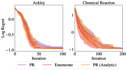
Figure 4: A comparison with an enumeration (gold standard) with respect to log regret.

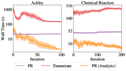
Figure 5: A comparison with enumeration with respect to wall time.

Appendix F Analysis of MC sampling in Probabilistic Reparameterization

The main text considers 1024 MC for PR. We consider 128, 256, and 512 samples, in addition to the default of 1024. For problems with discrete spaces that are enumerable, we also consider analytic PR. We do not find statistically significant differences between the final regret of any of these configurations (Figure 6). Run time is linear with respect to MC samples, and so substantial compute savings are possible when fewer MC samples are used (Figure 7). We observe comparable performance between PR with 1,024 MC samples and as few as 128 MC samples. With 64 or fewer MC samples, we observe performance degradation with respect to log regret in Figure 8, although wall time is considerably faster for fewer 64 or less MC samples as shown in Figure 9.

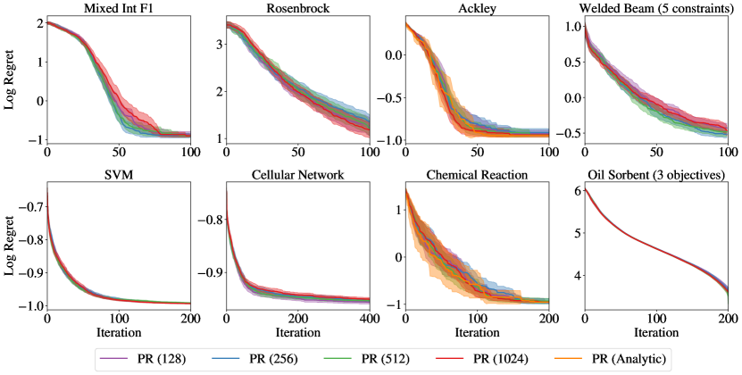
Figure 6: A sensitivity analysis of the optimization performance of PR with respect to the number of MC samples. We find that PR is robust to the number of MC samples, and that the performance of MC PR matches that of analytic PR.

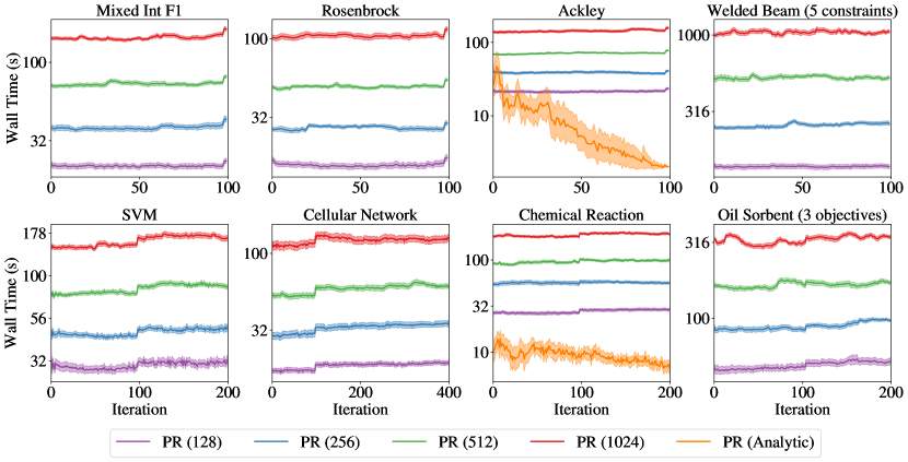
Figure 7: A sensitivity analysis of the wall time of PR with respect to the number of MC samples. We observe that wall time scales linearly with the number of MC samples, which is expected since we compute PR in $\frac{N}{32}$ chunks to avoid overflowing GPU memory.

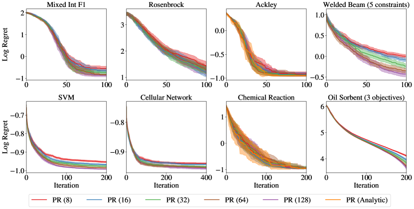
Figure 8: A sensitivity analysis of the optimization performance of PR with respect to a small number of MC samples (with samples between 8 and 64). Performance degrades slightly when few samples are used.

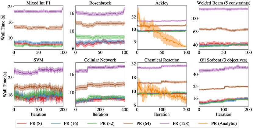
Figure 9: A sensitivity analysis of the wall time of PR with respect to the number of MC samples (with samples between 8 and 64). We observe that wall time scales linearly with the number of MC samples, which is expected since we compute PR in $\frac{N}{32}$ chunks to avoid overflowing GPU memory.

F.0.1 Evaluation of Approximation Error in MC Sampling

We examine the MC approximation error relative to analytic PR on the chemical reaction and ackley problems. The results in Figure 10 show the mean absolute percentage error (MAPE)

$$\frac{100}{|X_{\text{discrete}}|}\cdot\sum_{\bm{x}\in X_{\text{discrete}},\bm{\theta}\in\Theta_{\text{discrete}}}\frac{\mathbb{E}_{\bm{Z}\sim p(\bm{Z}|\bm{\theta})}\alpha(\bm{x},\bm{Z})-\frac{1}{N}\sum_{i=1}^{N}\alpha(\bm{x},\tilde{\bm{z}}_{i})}{\max_{\bm{x}\in X_{\text{discrete}},\bm{\theta}\in\Theta_{\text{discrete}}}\mathbb{E}_{\bm{Z}\sim p(\bm{Z}|\bm{\theta})}\alpha(\bm{x},\bm{Z})}$$

evaluated over a random set of $|X_{\text{discrete}}|=|\Theta_{\text{discrete}}|10,000$ points from $\mathcal{X}\times\mathcal{\Theta}$ (the sampled sets are denoted $X_{\text{discrete}},\Theta_{\text{discrete}}$). We observe a rapid reduction in MAPE as we increase the number of samples. With 1024 samples, MAPE is 0.055% (+/- 0.0002 %) over 20 replications (different MC samples in PR) on the chemical reaction problem and MAPE is 0.018% (+/- 0.0003 %) on the ackley problem.

With 128 samples, MAPE is 0.282% (+/- 0.0029 %) over 20 replications (different MC samples in PR) on the chemical reaction problem and MAPE is 0.052% (+/- 0.0021 %) on the ackley problem.

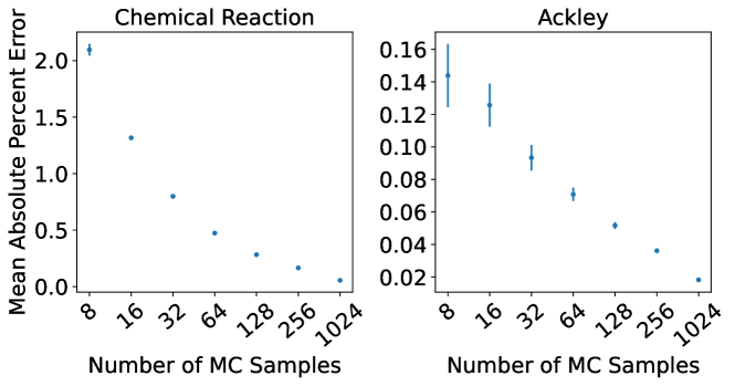
Figure 10: An evaluation of the mean absolute percentage error for the MC estimator of PR (relative to analytic PR).

Appendix G Effect of $\tau$ in Transformation

Throughout the main text, we use $\tau=0.1$, which we selected based on the observation that it provides a reasonable balance between retaining non-zero gradients of $g(\phi)$ with respect to $\phi$ and allowing $\theta$ to become close to 0 or 1 as shown in Figure 11.

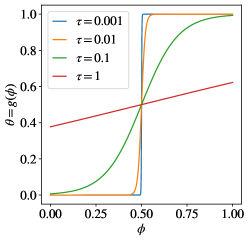
Figure 11: A comparison of the reparameterization of $\theta$ under various choices of $\tau$. We observe that $\tau=0.1$ provides a reasonable balance between retaining non-zero gradients of $g(\phi)$ with respect to $\phi$ and allowing $\theta$ to become close to 0 or 1.

As $\tau\rightarrow 0$, the $\theta$ can take more extreme values, but the gradient of the transformation with respect to $\phi$ also moves closer to zero. For larger values of $\tau$, the gradient of the transformation with respect to $\phi$ is larger, but $\theta$ has a more limited domain with less extreme values. We find that $\tau=0.1$ is a robust setting across all experiments.

Appendix H Alternative methods

H.1 Straight-through gradient estimators

An alternative approach to using approximating the gradients under exact rounding using finite differences is to approximate the gradients using straight-through gradient estimation (STE) [3]. The idea of STE is to approximate the gradient of a function with the identity function. In our setting, the gradient of the discretization function with respect to its input is estimated using an identity function. Using this estimator enables gradient-based AF optimization, even though the true gradient of the discretization function is zero everywhere that it is defined. Although STEs have been shown to work well empirically, these estimators are not well-grounded theoretically. Their robustness and potential pitfalls in the context of AF optimization have not been well studied. Below, we evaluate the aforementioned Exact Round + STE approach and show that it offers competitive optimization performance (Figure 12) with fast wall times (Figure 13), but does not quite match the optimization performance of PR on several benchmark problems.

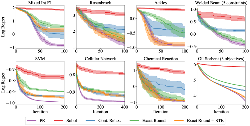
Figure 12: A comparison of exact rounding with straight-through gradient estimators versus other acquisition optimization strategies. Log regret on each problem. We report log hypervolume regret for Oil Sorbent and report the log regret of the best feasible objective for Welded beam.

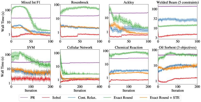
Figure 13: A comparison of wall times of exact rounding with straight-through gradient estimators versus other acquisition optimization strategies.

H.2 TR methods with alternative optimizers

In this section, we consider alternative methods to PR for optimizing AFs using within trust regions. The results in Figure 14 show that PR is a consistent best optimizer using TRs, but that STEs work quite well with TRs in many scenarios.

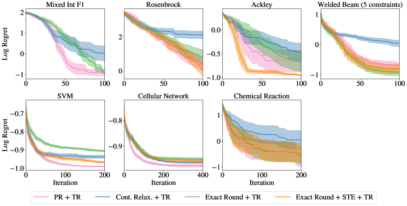
Figure 14: A comparison of TR methods with different acquisition optimization strategies. Log regret on each problem. We report log hypervolume regret for Oil Sorbent and report the log regret of the best feasible objective for Welded beam.

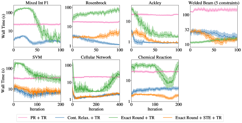
Figure 15: A comparison of wall times of TR methods with different acquisition optimization strategies.

Appendix I Acquisition Function Optimization at a Given Wall Time Budget

In Figure 16, we provide additional starting points (64 points, rather than 20) to other non-PR methods in order to provide them with additional wall-time budget. We find that using PR with 64 MC samples, PR provides rapid convergence compared to other baselines and therefore is a good optimization routine for any wall time budget.

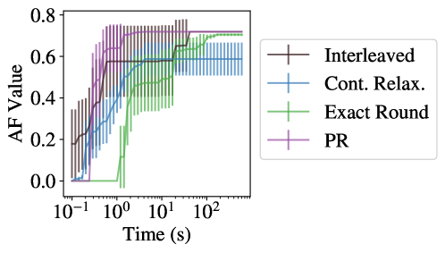
Figure 16: A comparison of methods for optimizing acquisition functions at a given wall time budget.

Appendix J Alternative categorical kernels

In this section, we demonstrate that PR can be used with arbitrary kernels over the categorical parameters including those that require discrete inputs (which Cont. Relax. is incompatible with). Specifically for the categorical parameters, we compare using (a) a Categorical kernel (default) versus with a Matérn-5/2 kernel with either (b) one-hot encoded categoricals, (c) a latent embedding kernel [67], or known embeddings based on density functional theory (DFT) [51]. For the latent embedding kernel, we follow Pelamatti et al. [44] and use a 1-d latent embedding for categorical parameters where the cardinality is less than or equal to 3 and a 2-d embedding for categorical parameters where the cardinality is greater than 3. For each latent embedding, we use an isotropic Matérn-5/2 kernel and use product kernel across the kernels for the categorical, binary, ordinal, and continuous parameters. For the kernel over DFT embeddings, we use the DFT embeddings for the direct arylation dataset from Shields et al. [51], which are available at https://github.com/b-shields/edbo. It is worth noting that in the Chemical Reaction problem, the black-box objective is a GP surrogate model with a Categorical kernel that is fit to the direct arylation dataset. The purpose of this section is demonstrate that PR is agnostic to the choice of kernel over discrete parameters. Because the Chemical Reaction problem is based on a GP surrogate, we do not draw conclusions about which choice of kernel is best suited for modeling the true, unknown underlying Chemical Reaction yield function.

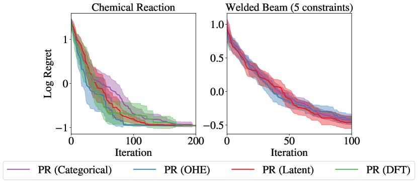
Figure 17: A comparison of different kernels over categorical parameters. Left: Welded beam has one categorical parameter, metal type (4 levels). Right: Chemical reaction has three categorical parameters, solvent, base, and ligand (with 4, 12, and 4 levels, respectively).

Appendix K Alternative Acquisition Functions

In this section, we compare PR with expected improvement (EI) against PR with upper confidence bound (UCB). For UCB, we set the hyperparameter $\beta$ in each iteration using the method in Kandasamy et al. [33]. Although UCB comes enjoys bounded regret [52], we find empirically that EI works better on most problems.

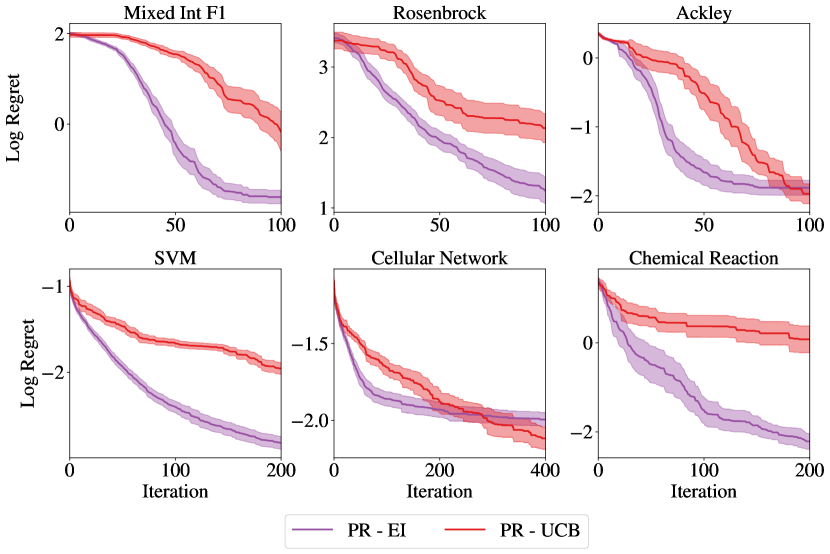
Figure 18: A comparison of expected improvement (EI) and upper confidence bound (UCB) acquisition functions with PR.

Appendix L Additional Results on Optimizing Acquisition Functions

In this section, we provide additional results on various approaches for optimizing acquisition functions using the same evaluation procedure as in the main text. We use 50 replications.

Figure 19: A comparison of methods for optimizing acquisition functions.

Appendix M Stochastic vs Deterministic Optimization

We compare optimizing PR with stochastic and deterministic optimization methods. For stochastic optimizers, we compare stochastic gradient ascent (SGA) and Adam with various initial learning rates. For SGA, the learning rate is decayed each time step $t$ by multiplying the initial learning rate by $t^{-0.7}$ and for Adam a fixed learning rate is used. For stochastic optimizers, the MC estimators of PR and its gradient stochastic mini-batches of $N=128$ MC samples are used. For deterministic optimization, base samples are kept fixed. All routines are run for a maximum of 200 iterations. In Figure 20, we observe that Adam is more robust to the choice of learning rate than SGA and generally is the best performing method. Furthermore, Adam consistently performs better than deterministic optimization. We compare Adam with a learning rate of $\frac{1}{40}$ against L-BFGS-B in Figure 21.

Figure 20: A comparison of PR using stochastic and deterministic optimization methods. The initial learning rate for stochastic gradient ascent is given in parentheses.

Figure 21: A comparison of optimizing the PO using deterministic estimation (via SAA) and optimization versus stochastic estimation and optimization.

Appendix N Comparison with an Evolutionary Algorithm

In Figures 22 and  22, we compare against the evolutionary algorithm PortfolioDiscreteOnePlusOne, which is the recommended algorithm for discrete and mixed search spaces in the Nevergrad package [45]. We find that PR significantly outperforms this baseline by a large margin with respect to log regret, but is slower than the evolutionary algorithm with respect to wall time.

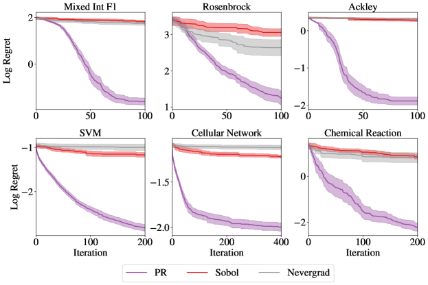
Figure 22: A comparison with an evolutionary algorithm with respect to log regret.

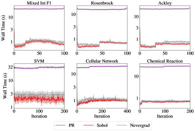
Figure 23: A comparison with an evolutionary algorithm with respect to wall time.

References

- Balandat et al. [2020] Maximilian Balandat, Brian Karrer, Daniel R. Jiang, Samuel Daulton, Benjamin Letham, Andrew Gordon Wilson, and Eytan Bakshy. Botorch: A framework for efficient monte-carlo Bayesian optimization. In Advances in Neural Information Processing Systems 33: Annual Conference on Neural Information Processing Systems 2020, NeurIPS 2020, December 6-12, 2020, virtual, 2020.
- Baptista and Poloczek [2018] Ricardo Baptista and Matthias Poloczek. Bayesian optimization of combinatorial structures. In Proc. of ICML, volume 80 of Proceedings of Machine Learning Research, pages 471–480. PMLR, 2018.
- Bengio et al. [2013] Yoshua Bengio, Nicholas Léonard, and Aaron Courville. Estimating or propagating gradients through stochastic neurons for conditional computation. ArXiv preprint, abs/1308.3432, 2013.
- Bergstra et al. [2011] James Bergstra, Rémi Bardenet, Yoshua Bengio, and Balázs Kégl. Algorithms for hyper-parameter optimization. In Advances in Neural Information Processing Systems 24: 25th Annual Conference on Neural Information Processing Systems 2011. Proceedings of a meeting held 12-14 December 2011, Granada, Spain, pages 2546–2554, 2011.
- Berkenkamp et al. [2019] Felix Berkenkamp, Angela P. Schoellig, and Andreas Krause. No-regret Bayesian optimization with unknown hyperparameters. Journal of Machine Learning Research, 20(50):1–24, 2019. URL http://jmlr.org/papers/v20/18-213.html.
- Bliek et al. [2021] Laurens Bliek, Arthur Guijt, Sicco Verwer, and Mathijs de Weerdt. Black-box mixed-variable optimisation using a surrogate model that satisfies integer constraints. GECCO ’21, page 1851–1859. Association for Computing Machinery, 2021.
- Boros and Hammer [2002] Endre Boros and Peter L. Hammer. Pseudo-boolean optimization. Discrete Applied Mathematics, 123(1):155–225, 2002. ISSN 0166-218X. doi: https://doi.org/10.1016/S0166-218X(01)00341-9.
- Daulton et al. [2020] Samuel Daulton, Maximilian Balandat, and Eytan Bakshy. Differentiable expected hypervolume improvement for parallel multi-objective bayesian optimization. In Advances in Neural Information Processing Systems 33: Annual Conference on Neural Information Processing Systems 2020, NeurIPS 2020, December 6-12, 2020, virtual, 2020.
- Daulton et al. [2021] Samuel Daulton, Maximilian Balandat, and Eytan Bakshy. Parallel Bayesian optimization of multiple noisy objectives with expected hypervolume improvement. In M. Ranzato, A. Beygelzimer, Y. Dauphin, P.S. Liang, and J. Wortman Vaughan, editors, Advances in Neural Information Processing Systems, volume 34, pages 2187–2200. Curran Associates, Inc., 2021.
- Daulton et al. [2022a] Samuel Daulton, Sait Cakmak, Maximilian Balandat, Michael A Osborne, Enlu Zhou, and Eytan Bakshy. Robust multi-objective Bayesian optimization under input noise. arXiv preprint arXiv:2202.07549, 2022a.
- Daulton et al. [2022b] Samuel Daulton, David Eriksson, Maximilian Balandat, and Eytan Bakshy. Multi-objective Bayesian optimization over high-dimensional search spaces. In Proceedings of the Thirty-Eighth Conference on Uncertainty in Artificial Intelligence, UAI 2022, Eindhoven, Netherlands, August 1-5, 2022, Proceedings of Machine Learning Research. AUAI Press, 2022b.
- Davies and Morton [2016] Huw ML Davies and Daniel Morton. Recent advances in c–h functionalization. The Journal of Organic Chemistry, 81(2):343–350, 2016.
- Daxberger et al. [2020] Erik A. Daxberger, Anastasia Makarova, Matteo Turchetta, and Andreas Krause. Mixed-variable Bayesian optimization. In Proceedings of the Twenty-Ninth International Joint Conference on Artificial Intelligence, IJCAI 2020, pages 2633–2639. ijcai.org, 2020. doi: 10.24963/ijcai.2020/365.
- Deshwal and Doppa [2021] Aryan Deshwal and Jana Doppa. Combining latent space and structured kernels for Bayesian optimization over combinatorial spaces. In M. Ranzato, A. Beygelzimer, Y. Dauphin, P.S. Liang, and J. Wortman Vaughan, editors, Advances in Neural Information Processing Systems, volume 34, pages 8185–8200. Curran Associates, Inc., 2021. URL https://proceedings.neurips.cc/paper/2021/file/44e76e99b5e194377e955b13fb12f630-Paper.pdf.
- Deshwal et al. [2021a] Aryan Deshwal, Syrine Belakaria, and Janardhan Rao Doppa. Bayesian optimization over hybrid spaces. In Proc. of ICML, volume 139 of Proceedings of Machine Learning Research, pages 2632–2643. PMLR, 2021a.
- Deshwal et al. [2021b] Aryan Deshwal, Syrine Belakaria, and Janardhan Rao Doppa. Mercer features for efficient combinatorial Bayesian optimization. In Thirty-Fifth AAAI Conference on Artificial Intelligence (AAAI), pages 7210–7218, 2021b.
- Dreifuerst et al. [2021] Ryan M Dreifuerst, Samuel Daulton, Yuchen Qian, Paul Varkey, Maximilian Balandat, Sanjay Kasturia, Anoop Tomar, Ali Yazdan, Vish Ponnampalam, and Robert W Heath. Optimizing coverage and capacity in cellular networks using machine learning. In ICASSP 2021-2021 IEEE International Conference on Acoustics, Speech and Signal Processing (ICASSP), pages 8138–8142. IEEE, 2021.
- Dua and Graff [2017] Dheeru Dua and Casey Graff. UCI machine learning repository, 2017.
- Duchon et al. [2004] Philippe Duchon, Philippe Flajolet, Guy Louchard, and Gilles Schaeffer. Boltzmann samplers for the random generation of combinatorial structures. Comb. Probab. Comput., 13(4–5):577–625, jul 2004. ISSN 0963-5483. doi: 10.1017/S0963548304006315.
- Emmerich et al. [2006] M. T. M. Emmerich, K. C. Giannakoglou, and B. Naujoks. Single- and multiobjective evolutionary optimization assisted by gaussian random field metamodels. IEEE Transactions on Evolutionary Computation, 10(4):421–439, 2006.
- Eriksson and Poloczek [2021] David Eriksson and Matthias Poloczek. Scalable constrained Bayesian optimization. In International Conference on Artificial Intelligence and Statistics, pages 730–738. PMLR, 2021.
- Eriksson et al. [2019] David Eriksson, Michael Pearce, Jacob R. Gardner, Ryan Turner, and Matthias Poloczek. Scalable global optimization via local Bayesian optimization. In Advances in Neural Information Processing Systems 32: Annual Conference on Neural Information Processing Systems 2019, NeurIPS 2019, December 8-14, 2019, Vancouver, BC, Canada, pages 5497–5508, 2019.
- Frazier [2018] Peter I Frazier. A tutorial on Bayesian optimization. ArXiv preprint, abs/1807.02811, 2018.
- Gardner et al. [2014] Jacob R. Gardner, Matt J. Kusner, Zhixiang Eddie Xu, Kilian Q. Weinberger, and John P. Cunningham. Bayesian optimization with inequality constraints. In Proc. of ICML, volume 32 of JMLR Workshop and Conference Proceedings, pages 937–945. JMLR.org, 2014.
- Garnett [2022] Roman Garnett. Bayesian Optimization. Cambridge University Press, 2022. in preparation.
- Garrido-Merchán and Hernández-Lobato [2020] Eduardo C. Garrido-Merchán and D. Hernández-Lobato. Dealing with categorical and integer-valued variables in Bayesian optimization with gaussian processes. Neurocomputing, 380:20–35, 2020.
- Glynn [1990] Peter W Glynn. Likelihood ratio gradient estimation for stochastic systems. Communications of the ACM, 33(10):75–84, 1990.
- Hansen et al. [2019] Nikolaus Hansen, Dimo Brockhoff, Olaf Mersmann, Tea Tusar, Dejan Tusar, Ouassim Ait ElHara, Phillipe R Sampaio, Asma Atamna, Konstantinos Varelas, Umut Batu, et al. Comparing continuous optimizers: numbbo/coco on github. 2019.
- Häse et al. [2021] Florian Häse, Matteo Aldeghi, Riley J Hickman, Loïc M Roch, and Alán Aspuru-Guzik. Gryffin: An algorithm for Bayesian optimization of categorical variables informed by expert knowledge. Applied Physics Reviews, 8(3):031406, 2021.
- Hutter et al. [2011] Frank Hutter, Holger H. Hoos, and Kevin Leyton-Brown. Sequential model-based optimization for general algorithm configuration. In Proceedings of the 5th International Conference on Learning and Intelligent Optimization, page 507–523. Springer-Verlag, 2011. ISBN 9783642255656.
- Jang et al. [2017] Eric Jang, Shixiang Gu, and Ben Poole. Categorical reparameterization with gumbel-softmax. In Proc. of ICLR. OpenReview.net, 2017.
- Jones et al. [1998] Donald R. Jones, Matthias Schonlau, and William J. Welch. Efficient global optimization of expensive black-box functions. Journal of Global Optimization, 13:455–492, 1998.
- Kandasamy et al. [2015] Kirthevasan Kandasamy, Jeff Schneider, and Barnabas Poczos. High dimensional Bayesian optimisation and bandits via additive models. In Francis Bach and David Blei, editors, Proceedings of the 32nd International Conference on Machine Learning, volume 37 of Proceedings of Machine Learning Research, pages 295–304, Lille, France, 07–09 Jul 2015. PMLR. URL https://proceedings.mlr.press/v37/kandasamy15.html.
- Kingma and Ba [2014] Diederik P Kingma and Jimmy Ba. Adam: A method for stochastic optimization. arXiv preprint arXiv:1412.6980, 2014.
- Kleijnen and Rubinstein [1996] Jack PC Kleijnen and Reuven Y Rubinstein. Optimization and sensitivity analysis of computer simulation models by the score function method. European Journal of Operational Research, 88(3):413–427, 1996.
- Liu et al. [2022] Sulin Liu, Qing Feng, David Eriksson, Benjamin Letham, and Eytan Bakshy. Sparse Bayesian optimization. arXiv preprint arXiv:2203.01900, 2022.
- Maddison et al. [2017] Chris J. Maddison, Andriy Mnih, and Yee Whye Teh. The concrete distribution: A continuous relaxation of discrete random variables. In Proc. of ICLR. OpenReview.net, 2017.
- Maddox et al. [2021] Wesley J Maddox, Maximilian Balandat, Andrew G Wilson, and Eytan Bakshy. Bayesian optimization with high-dimensional outputs. In Advances in Neural Information Processing Systems, volume 34, 2021.
- Mohamed et al. [2020] Shakir Mohamed, Mihaela Rosca, Michael Figurnov, and Andriy Mnih. Monte carlo gradient estimation in machine learning. J. Mach. Learn. Res., 21(132):1–62, 2020.
- Nguyen et al. [2020] Dang Nguyen, Sunil Gupta, Santu Rana, Alistair Shilton, and Svetha Venkatesh. Bayesian optimization for categorical and category-specific continuous inputs. In The Thirty-Fourth AAAI Conference on Artificial Intelligence, AAAI 2020, The Thirty-Second Innovative Applications of Artificial Intelligence Conference, IAAI 2020, The Tenth AAAI Symposium on Educational Advances in Artificial Intelligence, EAAI 2020, New York, NY, USA, February 7-12, 2020, pages 5256–5263. AAAI Press, 2020.
- Oh et al. [2019] ChangYong Oh, Jakub M. Tomczak, Efstratios Gavves, and Max Welling. Combinatorial Bayesian optimization using the graph cartesian product. In Advances in Neural Information Processing Systems 32: Annual Conference on Neural Information Processing Systems 2019, NeurIPS 2019, December 8-14, 2019, Vancouver, BC, Canada, pages 2910–2920, 2019.
- Owen [2003] Art B Owen. Quasi-monte carlo sampling. Monte Carlo Ray Tracing: Siggraph, 1:69–88, 2003.
- Paria et al. [2019] Biswajit Paria, Kirthevasan Kandasamy, and Barnabás Póczos. A flexible framework for multi-objective Bayesian optimization using random scalarizations. In Proceedings of the Thirty-Fifth Conference on Uncertainty in Artificial Intelligence, UAI 2019, Tel Aviv, Israel, July 22-25, 2019, volume 115 of Proceedings of Machine Learning Research, pages 766–776. AUAI Press, 2019.
- Pelamatti et al. [2021] Julien Pelamatti, Loïc Brevault, Mathieu Balesdent, El-Ghazali Talbi, and Yannick Guerin. Bayesian optimization of variable-size design space problems. Optimization and Engineering, 22(1):387–447, 2021.
- Rapin and Teytaud [2018] J. Rapin and O. Teytaud. Nevergrad - A gradient-free optimization platform. https://GitHub.com/FacebookResearch/Nevergrad, 2018.
- Rasmussen [2004] Carl Edward Rasmussen. Gaussian processes in machine learning. In Advanced Lectures on Machine Learning: ML Summer Schools 2003, Canberra, Australia, February 2 - 14, 2003, Tübingen, Germany, August 4 - 16, 2003, Revised Lectures, 2004.
- Robbins and Monro [1951] Herbert Robbins and Sutton Monro. A stochastic approximation method. The Annals of Mathematical Statistics, 22(3):400–407, 1951. ISSN 00034851.
- Ru et al. [2020] Bin Xin Ru, Ahsan S. Alvi, Vu Nguyen, Michael A. Osborne, and Stephen J. Roberts. Bayesian optimisation over multiple continuous and categorical inputs. In Proc. of ICML, volume 119 of Proceedings of Machine Learning Research, pages 8276–8285. PMLR, 2020.
- Russo and Roy [2014] Daniel Russo and Benjamin Van Roy. Learning to optimize via posterior sampling. arXiv preprint: arXiv 1301.2609, 2014.
- Samal et al. [2021] Soumya Ranjan Samal, Kaliprasanna Swain, Shuvabrata Bandopadhaya, Nikolay Dandanov, Vladimir Poulkov, Sidheswar Routray, and Gopinath Palai. Dynamic coverage optimization for 5g ultra-dense cellular networks based on their user densities. 2021.
- Shields et al. [2021] Benjamin J Shields, Jason Stevens, Jun Li, Marvin Parasram, Farhan Damani, Jesus I Martinez Alvarado, Jacob M Janey, Ryan P Adams, and Abigail G Doyle. Bayesian reaction optimization as a tool for chemical synthesis. Nature, 590(7844):89–96, 2021.
- Srinivas et al. [2010] Niranjan Srinivas, Andreas Krause, Sham M. Kakade, and Matthias W. Seeger. Gaussian process optimization in the bandit setting: No regret and experimental design. In Proc. of ICML, pages 1015–1022. Omnipress, 2010.
- The GPyOpt authors [2016] The GPyOpt authors. GPyOpt: A Bayesian optimization framework in python. http://github.com/SheffieldML/GPyOpt, 2016.
- Tran et al. [2019] Anh Tran, Minh Tran, and Yan Wang. Constrained mixed-integer gaussian mixture Bayesian optimization and its applications in designing fractal and auxetic metamaterials. Structural and Multidisciplinary Optimization, 59(6):2131–2154, 2019.
- Turner et al. [2021] Ryan Turner, David Eriksson, Michael McCourt, Juha Kiili, Eero Laaksonen, Zhen Xu, and Isabelle Guyon. Bayesian optimization is superior to random search for machine learning hyperparameter tuning: Analysis of the black-box optimization challenge 2020. In NeurIPS 2020 Competition and Demonstration Track, pages 3–26, 2021.
- Tušar et al. [2019] Tea Tušar, Dimo Brockhoff, and Nikolaus Hansen. Mixed-integer benchmark problems for single- and bi-objective optimization. In Proceedings of the Genetic and Evolutionary Computation Conference, GECCO ’19, page 718–726. Association for Computing Machinery, 2019.
- Wan et al. [2021] Xingchen Wan, Vu Nguyen, Huong Ha, Bin Xin Ru, Cong Lu, and Michael A. Osborne. Think global and act local: Bayesian optimisation over high-dimensional categorical and mixed search spaces. In Proc. of ICML, volume 139 of Proceedings of Machine Learning Research, pages 10663–10674. PMLR, 2021.
- Wan et al. [2022] Xingchen Wan, Cong Lu, Jack Parker-Holder, Philip J Ball, Vu Nguyen, Binxin Ru, and Michael Osborne. Bayesian generational population-based training. In ICLR Workshop on Agent Learning in Open-Endedness, 2022.
- Wang et al. [2020a] Boqian Wang, Jiacheng Cai, Chuangui Liu, Jian Yang, and Xianting Ding. Harnessing a novel machine-learning-assisted evolutionary algorithm to co-optimize three characteristics of an electrospun oil sorbent. ACS Applied Materials & Interfaces, 12(38):42842–42849, 2020a.
- Wang et al. [2020b] Jialei Wang, Scott C Clark, Eric Liu, and Peter I Frazier. Parallel Bayesian global optimization of expensive functions. Operations Research, 68(6):1850–1865, 2020b.
- Wang et al. [2017] Rui Wang, Jian Xiong, Hisao Ishibuchi, Guohua Wu, and Tao Zhang. On the effect of reference point in moea/d for multi-objective optimization. Applied Soft Computing, 58:25–34, 2017. ISSN 1568-4946. doi: https://doi.org/10.1016/j.asoc.2017.04.002.
- Williams [1992] Ronald J Williams. Simple statistical gradient-following algorithms for connectionist reinforcement learning. Machine learning, 8(3):229–256, 1992.
- Wilson et al. [2018] James T. Wilson, Frank Hutter, and Marc Peter Deisenroth. Maximizing acquisition functions for Bayesian optimization. In Advances in Neural Information Processing Systems 31: Annual Conference on Neural Information Processing Systems 2018, NeurIPS 2018, December 3-8, 2018, Montréal, Canada, pages 9906–9917, 2018.
- Yin et al. [2019] Mingzhang Yin, Yuguang Yue, and Mingyuan Zhou. ARSM: augment-reinforce-swap-merge estimator for gradient backpropagation through categorical variables. In Proc. of ICML, volume 97 of Proceedings of Machine Learning Research, pages 7095–7104. PMLR, 2019.
- Yin et al. [2020] Mingzhang Yin, Nhat Ho, Bowei Yan, Xiaoning Qian, and Mingyuan Zhou. Probabilistic Best Subset Selection by Gradient-Based Optimization. arXiv e-prints, 2020.
- Zhang and Golovin [2020] Richard Zhang and Daniel Golovin. Random hypervolume scalarizations for provable multi-objective black box optimization. In Proc. of ICML, volume 119 of Proceedings of Machine Learning Research, pages 11096–11105. PMLR, 2020.
- Zhang et al. [2019] Yichi Zhang, Siyu Tao, Wei Chen, and Daniel Apley. A latent variable approach to gaussian process modeling with qualitative and quantitative factors. Technometrics, 62:1–19, 07 2019. doi: 10.1080/00401706.2019.1638834.