Assessment of various Hamiltonian partitionings for the electronic structure problem on a quantum computer using the Trotter approximation

Abstract

Solving the electronic structure problem via unitary evolution of the electronic Hamiltonian is one of the promising applications of digital quantum computers. One of the practical strategies to implement the unitary evolution is via Trotterization, where a sequence of short-time evolutions of fast-forwardable (i.e. efficiently diagonalizable) Hamiltonian fragments is used. Given multiple choices of possible Hamiltonian decompositions to fast-forwardable fragments, the accuracy of the Hamiltonian evolution depends on the choice of the fragments. We assess efficiency of multiple Hamiltonian partitioning techniques using fermionic and qubit algebras for the Trotterization. Use of symmetries of the electronic Hamiltonian and its fragments significantly reduces the Trotter error. This reduction makes fermionic-based partitioning Trotter errors lower compared to those in qubit-based techniques. However, from the simulation-cost standpoint, fermionic methods tend to introduce quantum circuits with a greater number of T-gates at each Trotter step and thus are more computationally expensive compared to their qubit counterparts.

1 Introduction

Solving the electronic structure problem using controlled time evolution of quantum systems is one of the most promising applications of digital quantum computers. Ease of mapping fermionic operators to qubits using one of few existent mapping makes the second quantized formalism a convenient starting point. The molecular electronic Hamiltonian with $N$ single-particle spin-orbitals is

$$\hat{H}=\sum_{pq=1}^{N}h_{pq}\hat{a}^{\dagger}_{p}\hat{a}_{q}+\sum_{pqrs=1}^{N}g_{pqrs}\hat{a}^{\dagger}_{p}\hat{a}_{q}\hat{a}^{\dagger}_{r}\hat{a}_{s}$$ (1)

where $\hat{a}^{\dagger}_{p}$ ($\hat{a}_{p}$) is the creation (annihilation) fermionic operator for the $p$th spin-orbital, $h_{pq}$ and $g_{pqrs}$ are one- and two-electron integrals [1]. To obtain the spectrum of $H$ using digital quantum computers with error-correcting capability one can use the quantum phase estimation (QPE) algorithm. QPE involves unitary evolution generated by the system Hamiltonian $\exp[-it\hat{H}]$ to obtain the auto-correlation function and then Fourier transform (we will use atomic units throughout this work, $\hbar=1$).

One of the challenges of QPE is that $\exp[-it\hat{H}]$ cannot be implemented straightforwardly on a digital quantum computer. Within a fault-tolerant paradigm, several approaches have been put forward to address this problem: oracle query-based algorithms [2], quantum walks [3], qubitization [4], linear combination of unitaries [5] and product formulas [6]. We will refer to the last approach as Trotterization throughout this work. Trotterization starts with partitioning the Hamiltonian to exactly solvable or fast-forwardable parts, $\hat{H}_{n}$’s:

$$\hat{H}=\sum_{n=1}^{\Gamma}\hat{H}_{n}.$$ (2)

Using the Trotter approximation, $\exp[-it\hat{H}]$ can be expressed as a sequence of $e^{-i\hat{H}_{n}t}$ transformations for small $t$

$$e^{-it\hat{H}}=\prod_{n=1}^{\Gamma}e^{-it\hat{H}_{n}}+\mathcal{O}(t^{2}),$$ (3)

where time propagator operators $\exp[-it\hat{H}_{n}]$ can be translated to quantum gates easily. Implementation of $\exp[-it\hat{H}_{n}]$ propagators is straightforward because there are known unitary transformations $\hat{V}_{n}$ that bring $\hat{H}_{n}$ to operators diagonal in computational basis $\hat{D}_{n}$, $\hat{H}_{n}=\hat{V}_{n}^{\dagger}\hat{D}_{n}\hat{V}_{n}$. Due to non-commutativity of individual $\hat{H}_{n}$’s the Trotter error is proportional to commutator norms $||[\hat{H}_{n},\hat{H}_{n^{\prime}}]||$.

Even though Trotterization exhibits a steeper scaling of quantum circuit resources with target error compared to the rest of simulation approaches, it has two unique advantages compared to the so-called post-Trotter algorithms [7]: 1) lower overhead and the number of required ancilla qubits, and 2) the unique error scaling with the commutativity between the fast-forwardable Hamiltonian fragments, $\{\hat{H}_{n}\}$. The second property can be exploited in the simulation of physical systems where locality of interactions can be leveraged to reduce the number of non-zero commutators between Hamiltonian fragments.

Thus, Trotterized Hamiltonian simulation has been the subject of active research aiming at the reduction of the complexity of its associated quantum circuits in different physical systems [8, 9, 10, 11, 12].

There are several approaches to partitioning of molecular electronic Hamiltonians into exactly solvable fragments. Many of these approaches were developed in the measurement problem [13, 14, 15, 16, 17, 18] of the Variational Quantum Eigensolver (VQE) [19], where the partitioning is needed to obtain the expectation value of the Hamiltonian. A few of these partitioning techniques were considered for the Troterization problem [20, 17], yet different partitioning methods have not been compared systematically.

In this work, we consider Hamiltonian partitioning methods within two Hamiltonian realizations, which use fermionic and qubit operators, respectively. Although both realizations employ exactly solvable Hamiltonians, the structure of these Hamiltonians is different. In the fermionic case, the origin of solvability can be traced to the well-known solvability of hermitian one-electron Hamiltonians, while in the qubit case, the solvability is based on existence of Clifford group transformations that diagonalize any linear combination of commuting Pauli products.

For a Trotterization algorithm, the exponentials in approximate time evolution operator introduced in Eq. (3) are decomposed in terms of single-qubit rotations and Clifford gates. In an error-corrected algorithm such as surface code, Clifford gates can be implemented fault-tolerantly. Single-qubit-rotations, on the other hand, need to be compiled as a series of gates consisting of Clifford operations and at least one non-Clifford one, usually taken to be the T gate, a rotation around the $z$-axis by $\frac{\pi}{8}$ [21]. The implementation of T gates requires a procedure called magic state distillation [22], which renders T-gate synthesis the most costly aspect of error correction. The number of T gates required for a quantum algorithm is one of the essential efficiency determining parameters in fault-tolerant quantum computations. Thus, to determine which Hamiltonian partitioning approach is better, it is reasonable to compare the number of T gates required for performing the approximate unitary evolution.

The rest of the article is organized as follows. In section 2 we introduce the techniques used to analyze our Trotter error results for the different molecular systems and methods. Moreover, the main fermionic and qubit Hamiltonian partition schemes employed in our analysis are introduced. In the same section, we discuss the use of symmetries present in all Hamiltonian fragments that allow us to find tighter estimations of the Trotter error. Section 3 presents and discusses Trotter errors and T-gate estimates for different partitioning methods. Finally, Section 4 concludes by summarizing our most relevant results and giving the outlook.

2 Theory

2.1 Upper bounds for Trotter error

Equation (3) is a first order Trotter-Suzuki formula. Higher order Trotter approximations exist for $\exp[-it\hat{H}]$, which feature an error with steeper scaling with $t$, at the cost of increasing the number of products of exponentials [23]. For simplicity in our analysis, we focus on the error associated to the first-order Trotter formula. Here, the Trotter error can be written in terms of the spectral norm of the difference [11]

$$||e^{-it\hat{H}}-\prod_{n}e^{-it\hat{H}_{n}}||\leq\bar{\alpha}t^{2}/2,$$ (4)

where

$$\bar{\alpha}=\sum_{n}||[\hat{H}_{n},\sum_{n^{\prime}<n}\hat{H}_{n^{\prime}}]||.$$ (5)

To avoid order dependent parameter $\bar{\alpha}$ one can use the triangle inequality to upper bound it with a simpler quantity

$$2\sum_{n}||[\hat{H}_{n},\sum_{n^{\prime}<n}\hat{H}_{n^{\prime}}]||\leq\sum_{n,n^{\prime}}||[\hat{H}_{n},\hat{H}_{n^{\prime}}]||=\alpha.$$ (6)

For Trotter error analysis it is convenient to derive an upper bound on the commutator norm ($\alpha$) that contains properties of individual fragments. Such an upper bound can provide an insight on what properties of fragments define the success of a partitioning in lowering $\alpha$.

Using the triangle inequality

$$||[\hat{H}_{n},\hat{H}_{k}]||\leq 2||\hat{H}_{n}||\cdot||\hat{H}_{k}||$$ (7)

provides a loose upper bound. This bound can be further tightened by considering shifted Hamiltonians

$$\overline{\hat{H}}_{i}=\hat{H}_{i}-s_{i}\mathbf{\hat{I}},$$ (8)

where $s_{i}$ is a scalar, and $\mathbf{\hat{I}}$ is the identity operator. The shift introduced in Eq. (8) leaves the commutators between Hamiltonian fragments invariant

$$[\hat{H}_{i},\hat{H}_{j}]=[\overline{\hat{H}}_{i},\overline{\hat{H}}_{j}]$$ (9)

but changes the spectral norms, $||\overline{\hat{H}}_{i}||\neq||\hat{H}_{i}||$ by shifting the spectrum of $\hat{H}_{i}$ in Eq. (8). A tighter upper bound for $\alpha$ can be written as

$$\alpha = 2\sum_{i>j}||[\overline{\hat{H}}_{i},\overline{\hat{H}}_{j}]||\leq 4\sum_{i>j}||\overline{\hat{H}}_{i}||||\overline{\hat{H}}_{j}||$$ (10)

$$\leq 4\sum_{i>j}\min_{s_{i},s_{j}}||\overline{\hat{H}}_{i}||\cdot||\overline{\hat{H}}_{j}||.$$ (11)

Finding the minimum norm shifts can be done explicitly as

$$\min_{s_{i}}||\hat{H}_{i}-s_{i}\mathbf{I}||=\frac{\Delta E_{\text{i}}}{2},$$ (12)

where

$$\Delta E_{k}=\left(E_{\max,\text{k}}-E_{\min,k}\right)$$ (13)

is the spectral range for the $k$th Hamiltonian fragment and $E_{\max,k}$ ($E_{\min,k}$) is the maximum (minimum) eigenvalue of $H_{k}$. Then

$$\alpha\leq\sum_{i>j}\Delta E_{i}\Delta E_{j}=\beta,$$ (14)

constitutes the tightest upper bound for $\alpha$ among those involving triangle inequality for shifted Hamiltonian fragments, and it involves only spectral properties of individual fragments.

$\beta$ upper bound can be further analyzed using statistical quantities of fragment’s spectral ranges

$$\beta = \frac{1}{2}\left[\left(\sum_{i}\Delta E_{i}\right)^{2}-\sum_{i}\left(\Delta E_{i}\right)^{2}\right]$$ (15)

$$= \frac{1}{2}\left(\sum_{i}\Delta E_{i}\right)^{2}\left(1-\sum_{i}\omega_{i}^{2}\right),$$ (16)

where positive weights $\omega_{i}$ are defined as

$$\omega_{i} = \frac{\Delta E_{i}}{\sum_{k}\Delta E_{k}},\quad\omega_{i}\in[0,1].$$ (17)

Introducing weights $\omega_{i}$ allows us to recognize in the second factor of Eq. (16) the linearized entropy

$$S_{L}=1-\sum_{i}\omega_{i}^{2}.$$ (18)

Therefore, by denoting the first factor in Eq. (16) as $C=\sum_{i}\Delta E_{i}$ we obtain

$$\beta = \frac{1}{2}C^{2}S_{L}.$$ (19)

Reducing both $C$ and $S_{L}$ will decrease $\beta$. For reducing $C$ one needs to reduce $\Delta E_{i}$ of the fragments. $S_{L}$ can be decreased by selecting fragments with unevenly distributed weights.

Finding spectral ranges for exactly solvable problems is not always straightforward because one needs to find the largest and lowest eigenvalues among exponentially many. There exists an upper bound for $\Delta E/2$ that is based on $L_{1}$ norm of a coefficient vector for a linear combination of unitaries (LCU) decomposition for the corresponding operator [24]. Let us consider an LCU for $\hat{H}_{i}$

$$\hat{H}_{i}=\sum_{k}c_{k}^{(i)}\hat{V}_{k}+d_{i}\mathbf{\hat{I}},$$ (20)

where $\hat{V}_{k}$ are some unitaries, $c_{k}^{(i)}$ and $d_{i}$ are coefficients. Then, there is a following sequence of inequalities

$$\frac{\Delta E_{i}}{2}\leq||\hat{H}_{i}-d_{i}\mathbf{\hat{I}}||\leq\sum_{k}|c_{k}^{(i)}|,$$ (21)

where we used Eq. (12) in the first inequality and the triangle inequality with accounting for $||\hat{V}_{k}||=1$ in the second one. This upper bound suggests that fragments with lower LCU decomposition $L_{1}$ norms can be better candidates for reducing the Trotter error.

2.2 T-gate estimates

Time-energy uncertainty principle requires propagation for longer time to reach higher accuracy in the energy estimation. The Trotter error bound in Eq. (4) for a single Trotter step can be extended to multiple steps, $N_{s}$

$$\epsilon=||e^{-iT\hat{H}}-\left(\prod_{n}e^{-it\hat{H}_{n}}\right)^{N_{s}}||\leq\frac{\alpha T^{2}}{N_{s}},$$ (22)

where $T=N_{s}t$ is the simulation time. Here, we used the fact that the overall error from repeating the first-order Trotter sequence $N_{s}$ times accumulates at most linearly with $N_{s}$ [25]. The Trotter error $\alpha$ is an important figure of merit for the estimation of quantum resources. The number of Trotter steps to reach the level of accuracy $\epsilon$ while keeping $T$ fixed is $N_{s}\leq\alpha T^{2}/\epsilon$, so lowering $\alpha$ would allow to take longer and fewer time-steps to cover $T$.

The number of T-gates will be proportional to $N_{s}$ multiplied by the number of T-gates required for each time-step. For comparison of different partitioning methods we will only use system independent characteristics, such as the product $\alpha N_{R}$, where $N_{R}=\sum_{i=1}^{\Gamma}N_{R}^{(i)}$ is the number of single-qubit rotations needed in each Trotter step obtained as a sum over the number of single-qubit rotations for each Hamiltonian fragment $N_{R}^{(i)}$. The number of single-qubit rotations with arbitrary angles is proportional to the number of T gates, where the coefficient of proportionality can depend on a particular compiling scheme [26, 27].

In Appendix A we develop an analysis of the T-gate count for Adaptive QPE eigenvalue estimation for a fixed target error, considering relevant sources of error in addition to the Trotter approximation. This was done with the purpose of showing that the figure of merit $\alpha N_{R}$ suffices to compare the resource-efficiency of the different Hamiltonian decomposition methods addressed in this work.

2.3 Fermionic partitioning methods

These methods are based on solvability of one-electron Hamiltonians using orbital rotations, for a one-electron part of the electronic Hamiltonian we can write

$$\hat{h}_{\rm 1e} = \sum_{pq}h_{pq}\hat{a}^{\dagger}_{p}\hat{a}_{q}=\hat{U}^{\dagger}\left(\sum_{p}\epsilon^{(1)}_{p}\hat{n}_{p}\right)\hat{U},$$ (23)

where $\hat{n}_{p}=\hat{a}^{\dagger}_{p}\hat{a}_{p}$ occupation number operators, $\epsilon_{p}$ are real constants, and $\hat{U}$ are orbital rotation transformations

$$\hat{U}=\prod_{p>q}e^{\theta_{pq}(\hat{a}^{\dagger}_{p}\hat{a}_{q}-\hat{a}^{\dagger}_{q}\hat{a}_{p})}.$$ (24)

Note that $\hat{n}_{p}$ form a largest commuting subset of $\{\hat{a}^{\dagger}_{p}\hat{a}_{q}\}$ operators, $[\hat{n}_{p},\hat{n}_{q}]=0$, and they are directly mapped to polynomial functions of Pauli-$\hat{z}$ operators by all standard fermion-qubit mappings [28]. Orbital rotations $\hat{U}$ form a continuous Lie group, $\hat{U}_{1}\hat{U}_{2}=\hat{U}_{3}$, therefore, even though different exponential operators in Eq. (24) do not commute, one can write each $\hat{U}$ using different orders. This will only require adjusting corresponding amplitudes $\theta_{pq}$.

Two-electron Hamiltonians that are exact squares of one-electron Hamiltonians also can be solved by orbital rotations

$$\hat{H}^{(LR)} = \left(\sum_{pq}{\tilde{h}}_{pq}\hat{a}^{\dagger}_{p}\hat{a}_{q}\right)^{2}=\hat{U}^{\dagger}\left(\sum_{p}{\tilde{\epsilon}}_{p}\hat{n}_{p}\right)^{2}\hat{U}$$ (25)

$$= \hat{U}^{\dagger}\left(\sum_{p,q}{\tilde{\epsilon}}_{p}{\tilde{\epsilon}}_{q}\hat{n}_{p}\hat{n}_{q}\right)\hat{U}.$$ (26)

Formally, ${\tilde{\epsilon}}_{p}{\tilde{\epsilon}}_{q}$ can be considered as an entry of a rank-deficient matrix, this consideration suggests that one can substitute it in principle by a full-rank hermitian matrix, $\lambda_{pq}$, without loss of solvability. Thus a more general two-electron Hamiltonian that can be solved by orbital rotations has a form

$$\hat{H}^{\rm(FR)}=\hat{U}^{\dagger}\left(\sum_{p,q}\lambda_{pq}\hat{n}_{p}\hat{n}_{q}\right)\hat{U}.$$ (27)

Note that if $\lambda_{pq}$ is a diagonal matrix $\hat{H}^{\rm(FR)}$ can describe purely one-electron Hamiltonians, this is in contrast with a rank-deficient case where ${\tilde{\epsilon}}_{p}{\tilde{\epsilon}}_{q}$ can encode purely one-electron Hamiltonians if ${\tilde{\epsilon}}_{p}$ has only a single non-zero component. Further generalization of two-electron Hamiltonians solvable by orbital rotations is done in Ref. [29], but it follows the idea of having different eigenstates obtained by different orbital rotations and is not as straightforward to use as forms in Eq. (27) and Eq. (26).

Low-rank (LR) decomposition: This method uses orbital rotations to diagonalize the one-electron part and to represent the two-electron part of Eq. (1) as a linear combination of Eq. (26) fragments [17]

$$\hat{H} = \hat{h}_{\text{1e}}+\sum_{l=2}^{\Gamma}\hat{H}_{l}^{(\text{LR})},$$ (28)

where

$$\hat{h}_{\text{1e}} = \hat{U}_{1}^{\dagger}\left(\sum_{p}\epsilon_{p}^{(1)}\hat{n}_{p}\right)\hat{U}_{1}=\sum_{pq}h_{pq}\hat{a}^{\dagger}_{p}\hat{a}_{q}$$ (29)

$$\hat{H}_{l}^{(\text{LR})} = \hat{U}_{l}^{\dagger}\left(\sum_{p,q}\epsilon_{p}^{(l)}\epsilon_{q}^{(l)}\hat{n}_{p}\hat{n}_{q}\right)\hat{U}_{l}.$$ (30)

One computational advantage of this low-rank decomposition is that it can be done by diagonalizing the two-electron tensor $g_{pq,rs}$ considered as a matrix where each dimension is spanned by a pair of basis indices. This diagonalization gives a theoretical limit on $\Gamma\leq N(N+1)/2$, where less sign corresponds to a truncation of the expansion by removing terms for low magnitude eigenvalues. Further details of this decomposition procedure can be found in Ref. [17].

Full-rank (FR) optimization: Using fragments of Eq. (27) leads to the FR optimization (FRO)

$$H = \hat{h}_{\text{1e}}+\sum_{l=2}^{\Gamma}\hat{H}_{l}^{(\text{FR})},$$ (31)

where

$$\hat{H}_{l}^{(\text{FR})} = \hat{U}_{l}^{\dagger}\left(\sum_{i,j}^{N}\lambda_{ij}^{(l)}\hat{n}_{i}\hat{n}_{j}\right)\hat{U}_{l}.$$ (32)

In practice, the set $\{\hat{H}_{l}^{(\text{FR})}\}$ can be found by minimizing the $L_{1}$ norm of the $\mathbf{G}$ tensor (under a given numerical threshold) in

$$\sum_{pqrs}^{N}g_{pqrs}\hat{a}^{\dagger}_{p}\hat{a}_{q}\hat{a}^{\dagger}_{r}\hat{a}_{s} - \sum_{l=2}^{\Gamma}\hat{U}_{l}^{\dagger}(\mathbf{\theta}^{(l)})\left(\sum_{i,j}^{N}\lambda_{ij}^{(l)}\hat{n}_{i}\hat{n}_{j}\right)\hat{U}_{l}(\mathbf{\theta}^{(l)})$$ (33)

$$= \sum_{prqs=1}^{N}G_{pqrs}\hat{a}^{\dagger}_{p}\hat{a}_{q}\hat{a}^{\dagger}_{r}\hat{a}_{s}$$

over the space of the variables $\{\mathbf{\theta}^{(l)}\}$ that parameterize the $\{\hat{U}_{l}\}$ unitaries, as well as the $\{\lambda_{ij}^{(l)}\}$ variables [18].

A computationally more efficient variant of FR decomposition consists of an iterative greedy strategy, which at the $i^{\rm th}$ iteration ($i\geq 1$) finds the single optimal Hamiltonian fragment $\hat{H}_{i+1}^{(\text{FR})}$ that minimizes the $L_{1}$ norm of tensor $\tilde{\mathbf{G}}^{(i+1)}$:

$$\sum_{pqrs=1}^{N}\tilde{G}_{pqrs}^{(i)}\hat{a}^{\dagger}_{p}\hat{a}_{q}\hat{a}^{\dagger}_{r}\hat{a}_{s}-\hat{H}_{i+1}^{(\text{FR})}=\sum_{prqs=1}^{N}\tilde{G}_{pqrs}^{(i+1)}\hat{a}^{\dagger}_{p}\hat{a}_{q}\hat{a}^{\dagger}_{r}\hat{a}_{s},$$ (34)

where $\tilde{G}_{pqrs}^{(1)}=g_{pqrs}$. Iterations are carried out until the $L_{1}$ norm of $\tilde{\mathbf{G}}^{(i+1)}$ is below a given threshold. The outlined scheme will be referred as greedy FR optimization (GFRO). It yields larger norm Hamiltonian fragments in the beginning of the process and smaller norm ones at the end, which generally lowers the entropic part of Eq. (19) compared to other FR decomposition approaches.

Initial Hamiltonian: Historically, one-electron part of the electronic Hamiltonian was treated separately from the two-electron part [17, 18]. However, one can add the one electron contributions to the two-electron part by modifying the $g_{pq,rs}$ tensor. There are several ways to do this, one of the simplest approaches is to transform the entire Hamiltonian in the orbital frame where the one-electron part ($\hat{h}_{\text{1e}}$) is diagonal

$$\hat{U}_{1}\hat{H}\hat{U}_{1}^{\dagger} = \sum_{p}\epsilon_{p}\hat{n}_{p}+\sum_{pq,rs}\tilde{g}_{pq,rs}\hat{a}^{\dagger}_{p}\hat{a}_{q}\hat{a}^{\dagger}_{r}\hat{a}_{s}$$ (35)

$$\hat{H} = \hat{U}_{1}^{\dagger}\left(\sum_{pq,rs}[\tilde{g}_{pq,rs}+\epsilon_{p}\delta_{pq}\delta_{pr}\delta_{ps}]\hat{a}^{\dagger}_{p}\hat{a}_{q}\hat{a}^{\dagger}_{r}\hat{a}_{s}\right)\hat{U}_{1}$$ (36)

$$= \sum_{p^{\prime}q^{\prime},r^{\prime}s^{\prime}}\bar{g}_{p^{\prime}q^{\prime},r^{\prime}s^{\prime}}\hat{a}^{\dagger}_{p^{\prime}}\hat{a}_{q^{\prime}}\hat{a}^{\dagger}_{r^{\prime}}\hat{a}_{s^{\prime}},$$

where primed indices correspond to orbitals after the $\hat{U}_{1}$ conjugation. Using the augmented $\bar{g}_{p^{\prime}q^{\prime},r^{\prime}s^{\prime}}$ tensor one can do either the LR or FR decompositions. In particular, we consider in this work GFRO for the Hamiltonian in Eq. (36), which we termed SD-GFRO, where SD stands for "Singles and Doubles", as a reference to single and double excitation operators commonly used in electronic structure literature.

Fragments post-processing: After obtaining solvable fragments $\{\hat{H}_{l}\}$ one has a freedom to extract one-electron parts from each fragment

$$\hat{H}_{l} = \hat{U}_{l}^{\dagger}\left(\sum_{pq}\lambda^{(l)}_{pq}\hat{n}_{p}\hat{n}_{q}\right)\hat{U}_{l}$$ (37)

$$= \hat{U}_{l}^{\dagger}\left(\sum_{p}f^{(l)}_{p}\hat{n}_{p}\right)\hat{U}_{l}$$

$$+ \hat{U}_{l}^{\dagger}\left(\sum_{pq}[\lambda^{(l)}_{pq}-\delta_{pq}f^{(l)}_{p}]\hat{n}_{p}\hat{n}_{q}\right)\hat{U}_{l},$$

where the single index sum corresponds to the $p=q$ part and simplifies to a one-electron contribution due to $n_{p}^{2}=n_{p}$, and $f^{(l)}_{p}$ are free parameters that can be optimized. Here, $\lambda^{(l)}_{pq}$ can be either full-rank or rank-deficient depending on what scheme is used for the decomposition. This consideration allows one to sum all the one-electron parts from all fragments to obtain a new single solvable one-electron fragment

$$\hat{h}_{\text{1e}}+\sum_{l}\hat{U}_{l}^{\dagger}\left(\sum_{p}f^{(l)}_{p}\hat{n}_{p}\right)\hat{U}_{l}=$$

$$\hat{U}^{\dagger}\left(\sum_{p}\tilde{\lambda}_{pp}\hat{n}_{p}\right)\hat{U}.$$ (38)

The new Hamiltonian decomposition becomes

$$\hat{H} = \hat{U}^{\dagger}\left(\sum_{p}\tilde{\lambda}_{pp}\hat{n}_{p}\right)\hat{U}$$ (39)

$$+ \sum_{l}\hat{U}_{l}^{\dagger}\left(\sum_{pq}[\lambda_{pq}^{(l)}-\delta_{pq}f^{(l)}_{p}]\hat{n}_{p}\hat{n}_{q}\right)\hat{U}_{l}.$$

A possible advantage of this regrouping can come from potential cancellation of contributions within the single one-electron term so that the spectral range of the new one-electron term is reduced and reduction of spectral norms for two-electron terms after removing the diagonal parts. Optimizing parameters $f^{(l)}_{p}$ was performed successfully for the measurement problem in the VQE framework [30], yet similar optimization for the Trotter error runs into computational challenges associated with accurate prediction of fragment spectral range dependence on $f^{(l)}_{p}$. Due to this difficulty we employed a heuristic approach that is based on the connection between a fragment spectral range and an $L_{1}$ norm for its LCU decomposition (see Eq. (21)).

The idea of the heuristic approach is to use fragments whose LCU decomposition has low $L_{1}$ norm, such fragments can be obtained with a particular choice of $f^{(l)}_{p}$. It was found in Ref. [31] that substitution of every $\hat{n}_{i}$ operator in two-electron parts by reflection $\hat{r}_{i}=(1-2\hat{n}_{i})$ ($\hat{r}_{i}^{2}=1$ and $\hat{r}_{i}^{\dagger}=\hat{r}_{i}$) reduces the $L_{1}$ norm of a collection of solvable fragments. This substitution will require adjustment of coefficients and addition of one electron terms

$$H = \sum^{N}_{pq=1}\tilde{h}_{pq}a^{\dagger}_{p}\hat{a}_{q}$$ (40)

$$+ \sum_{k=2}\hat{U}_{k}^{\dagger}\left(\sum_{i,j}^{N}\frac{\lambda_{ij}^{(k)}}{4}\hat{r}_{i}\hat{r}_{j}\right)\hat{U}_{k}$$

$$- \frac{1}{4}\sum_{p,q}g_{pp,qq},$$

where

$$\tilde{h}_{pq}=h_{pq}+\sum_{k}g_{pq,kk}.$$ (41)

This procedure reduces four-fold the two-body tensor within the Hamiltonian fragments which generally leads to a decrease of their respective spectral norms. Circuit analysis: To estimate the number of T-gates we provide the estimate for the number of single-qubit rotation gates for all fermionic Hamiltonian partition schemes considered here. The implementation of the Hamiltonian (first-order) Trotter step is

$$\prod_{n=1}^{\Gamma}e^{-i\hat{H}_{n}t}=\hat{U}^{\dagger}_{1}e^{-i\sum_{p}\epsilon^{(1)}_{p}\hat{n}_{p}}\hat{U}_{1}\prod_{l=2}^{\Gamma}\hat{U}_{l}^{\dagger}e^{-it\sum_{i,j}^{N}\lambda_{ij}^{(l)}\hat{n}_{i}\hat{n}_{j}}\hat{U}_{l}$$ (42)

where adjacent unitary spin-orbital rotations can be combined using the Lie group closure $\hat{U}_{l}\hat{U}_{l+1}^{\dagger}=\hat{U}_{l,l+1}$, $\hat{U}_{l,l+1}$ has the form of Eq. (24) with $N(N-1)/2$ one-electron generators. Each of these $\hat{U}_{l,l+1}$ rotations, can be decomposed as a set of $N(N-1)/2$ rotations that contain 2 arbitrary amplitude single-qubit rotations and Clifford transformations [9, 17]. Similarly, the circuit implementation for the simulation of the $\exp\left(-it\sum_{i,j}^{N}\lambda_{ij}^{(l)}\hat{n}_{i}\hat{n}_{j}\right)$ (note that $\lambda_{ij}^{(l)}=\epsilon_{i}^{(l)}\epsilon_{j}^{(l)}$ for LR) is accomplished with at most $N(N+1)/2$ two-qubit gates, where the compilation of each one of the latter entails the implementation of 2 single-qubit rotations. Finally, the implementation of $\exp\left(-i\sum_{p}\epsilon^{(1)}_{p}\hat{n}_{p}\right)$ requires at most $N$ single qubit rotations. From these considerations and taking into account that a single Trotter step requires the implementation of $\Gamma+1$ orbital rotations, it follows that the total single rotation gate count is no larger than $2N^{2}\Gamma-N$.

2.4 Qubit partitioning methods

Qubit realizations of the electronic Hamiltonian are obtained after applying one of the fermion-qubit mappings [32, 33]

$$\hat{H}_{q}=\sum_{n}c_{n}\hat{P}_{n},\quad\hat{P}_{n}=\otimes_{k=1}^{N}\hat{\sigma}_{k}^{(n)}$$ (43)

where $c_{n}$ are numerical coefficients and $\hat{P}_{n}$ are tensor products of single-qubit Pauli operators and the identity, $\hat{\sigma}_{k}^{(n)}=\hat{x}_{k},\hat{y}_{k},\hat{z}_{k},\hat{I}_{k}$, acting on the $k$th qubit.

Fully-commuting (FC) grouping: This approach partitions $\hat{H}_{q}$ into $\hat{H}_{n}^{(\text{FC})}$ fragments containing commuting Pauli products: if $\hat{P}_{I},\hat{P}_{J}\in\hat{H}_{n}^{(\text{FC})}$ then $[\hat{P}_{I},\hat{P}_{J}]=0$. This commutativity condition guarantees that $\hat{H}_{n}^{(\text{FC})}$ can be rotated into a linear combination of $\hat{z}_{i}$ operator products by a sequence of Clifford group transformations [16, 34]. We will be referring to it as the fully-commuting qubit partitioning scheme, mainly because it was developed for the VQE measurement problem where “fully" was added to its name to separate it from a more restrictive qubit-wise commuting scheme [15].

The problem of finding the minimum number of fragments $\{\hat{H}_{n}^{(\text{FC})}\}$ representing the Hamiltonian $\hat{H}_{q}$ has been shown to be equivalent to a Minimum Clique Cover (MCC) problem for a graph representing the Hamiltonian. For this graph each term of $\hat{H}_{q}$ is a vertex and the commutativity condition determines connectivity [16, 15]. The MCC problem is NP-hard but it was found that different heuristic polynomial-in-time algorithms can find good approximate solutions. In this work we specifically consider the largest-first (LF) heuristic, whose name makes a reference to the ordering which the algorithm uses to process the vertices of the Hamiltonian graph [16, 15]; as well as the Sorted Insertion (SI) algorithm [35]. The latter is a greedy algorithm introduced to reduce the number of measurements required to attain a given level of accuracy in the estimation of the energy expectation value (or any other observable), rather than aiming at the minimization of the number of groups in the Hamiltonian partition.

Circuit analysis: Here we analyze the number of single-qubit rotations as a proxy for the number of T-gates. For both qubit commutativity grouping schemes, the first order Trotter propagator can be implemented as

$$\prod_{n=1}^{\Gamma}e^{-it\hat{H}_{n}}=\prod_{n=1}^{\Gamma}[\hat{U}_{n}^{\dagger}e^{-it\hat{Z}_{n}}\hat{U}_{n}]$$ (44)

where $\hat{Z}_{n}$ is a linear combination of Pauli products of $\hat{z}_{i}$ operators, and $\hat{U}_{n}$ are single- and two-qubit Clifford transformations for the FC scheme. Due to the Clifford character, $\hat{U}_{n}$’s do not contribute to the T-gate count. The number of $e^{-it\hat{Z}_{n}}$ terms scale as $\mathcal{O}(N^{3})$ while the total number of single-qubit rotations will be the same as the total number of Pauli products in the Hamiltonian, $\mathcal{O}(N^{4})$ [16].

For a summary of the Hamiltonian decomposition methods considered in this work, we refer the reader to Table 1.

Method	Partition Encoding	Algorithm character	Extra-processing	Refs.
FC-LF	Qubit	Non-greedy	-	[15]
FC-SI	Qubit	Greedy	-	[15],[16],[20]
LR	Fermionic	-	-	[17]
LR-LCU	Fermionic	-	Post-processing	[24]
FRO	Fermionic	Non-greedy	-	[18]
GFRO	Fermionic	Greedy	-	[18]
GFRO-LCU	Fermionic	Greedy	Post-processing	[24]
SD-GFRO	Fermionic	Greedy	Pre-processing	[24]

Table 1: Summary of the Hamiltonian decomposition methods considered in this work, alongside the type of encoding employed in the partition (fermionic or qubit-based), the character of the algorithm (greedy, non-greedy) and whether the scheme includes extra-processing of the Hamiltonian previous or after its decomposition.

2.5 Use of symmetries for Trotter error estimation

We can exploit symmetries shared by all Hamiltonian fragments pertaining to the same partition to introduce tighter estimations of the first-order Trotter error. In practice, Hamiltonian simulation can be performed on an initial state belonging to one of the symmetry group irreducible representations [36]. Therefore, $\alpha$ can be estimated by considering only the subspace of the Hilbert space corresponding to the irreducible representation of interest.

Here, we extended the approach developed in Ref. [36], where estimations of Trotter error are based on fermionic norms for particle-number preserving operators $\{\hat{X}\}$ ($[\hat{X},\hat{N}]=0$, $\hat{N}$ is the total-particle number operator). These norms are equal to the spectral norm of the observables defined on manifolds spanned by eigenstates of the total particle-number operator ($\hat{N}|\psi_{\eta}\rangle=\eta|\psi_{\eta}\rangle$):

$$||\hat{X}||_{\eta}=\underset{|\psi_{\eta}\rangle}{\text{max}}\sqrt{\langle\psi_{\eta}|\hat{X}^{\dagger}\hat{X}|\psi_{\eta}\rangle}.$$ (45)

It is straightforward to generalize this metric to include the spin symmetries $\hat{S}_{z}$ (projection of the total electronic spin angular momentum along $z$) and $\hat{S}^{2}$ (the square of the norm of the total electronic spin angular momentum) for the fermionic partition approaches. Consequently, the projected Trotter error is performed on manifolds that are spanned by states ${|\psi_{\eta,m,s}\rangle}$ which are simultaneous eigenstates of $\hat{N}$, $\hat{S}_{z}$ and $\hat{S}^{2}$, with eigenvalues $\eta$, $m$ and $s(s+1)$, respectively. Similarly, for qubit-based methods, it is possible to find qubit symmetries $\{\hat{Q}_{i}\}$ that satisfy $[\hat{Q}_{i},\hat{H}_{n}]=0$ $\forall n$ [see Eq. (2)]. A general search for these qubit symmetries can be computationally expensive. Therefore we restrict our consideration only to a single Pauli product symmetries, they can be found efficiently using techniques developed for the qubit tapering [37].

For the Trotter analysis we introduce

$$\alpha_{\mathbf{Q}}=\sum_{n_{1},n_{2}}||[\hat{H}_{n_{2}},\hat{H}_{n_{1}}]||_{\mathbf{Q}}.$$ (46)

where $\mathbf{Q}$ labels the set of quantum numbers that define the manifold the Trotter error is projected on. Thus, for fermionic methods we have $\mathbf{Q}=[n,m,s]$ whereas for qubit-based schemes $\mathbf{Q}=[\zeta_{1},\zeta_{2},\dots,\zeta_{n}]$, where $\zeta_{i}$ labels one of the eigenvalues of the $i$th qubit symmetry $\hat{Q}_{i}$. Symmetry constraints are straightforwardly extended to the $\beta$ spectral range upper bound for $\alpha$

$$\beta_{\mathbf{Q}}=\Delta E_{i,\mathbf{Q}}\Delta E_{j,\mathbf{Q}}\geq\alpha_{\mathbf{Q}},$$ (47)

where $\Delta E_{i,\mathbf{Q}}$ is the spectral range of the symmetric manifold with quantum numbers $\mathbf{Q}$ for $\hat{H}_{i}$.

3 Results and discussion

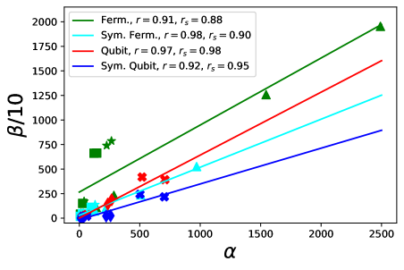
Figure 1: Correlations between $\alpha$ and its upper bound $\beta$ [Eqs. (5) and (11)] for fermionic (green) and qubit (red) methods. The correlation between the symmetry-projected counterparts $\alpha_{\mathbf{Q}}$ and $\beta_{\mathbf{Q}}$ [see Eqs. (46) and (47)] are shown in cyan and blue for fermionic and qubit methods, respectively. The fermionic methods considered are FRO (triangles), GFRO (squares) and LR (stars), whereas the qubit partition methods are FC LF (crosses) and FC SI (diamonds). The straight lines are obtained by a least-square fit, their Pearson ($r$) and Spearman ($r_{s}$) coefficients are indicated in the legend.

We considered the partition schemes described in the Methods section for the electronic Hamiltonians corresponding to molecules H₂, LiH, BeH₂, H₂O and NH₃. The latter were generated using the STO-3G basis and the Bravyi-Kitaev transformations (for the qubit encodings) as implemented in the OpenFermion package [38]. The nuclear geometries for the molecules are given by R(H-H)=1 Å (H₂), R(Li-H)=1 Å (LiH) and R(Be-H)=1 Å with collinear atomic arrangement (BeH₂), R(O-H)=1 Å and $\angle$HOH=107.6^∘ (H₂O); and R(N-H)=1 Å with $\angle$HNH=107^∘ (NH₃).

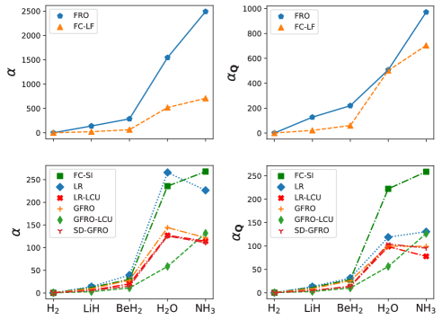
Figure 2: Left panels: trends in Trotter errors $\alpha$ (in squared Hartrees) for the different Hamiltonian partitionings. Right panels: trends in symmetry-projected Trotter errors $\alpha_{\mathbf{Q}}$ (in squared Hartrees). For the fermionic methods we consider $\alpha_{\eta,m,s}$ [see Eq. (46)] with $\eta$ corresponding to the number of electrons of the neutral molecule, and $m=s=0$. For the qubit-based methods, we consider $\alpha_{\mathbf{Q}}$ [see Eq. (46)] in the subspace of qubit symmetries corresponding to the ground state of the neutral molecule.For clarity and to highlight the difference in the scale of the non-greedy algorithms with respect to the rest of the methods, we show FRO and FC-LF results in different plots.

3.1 Trotter errors

Here we explore the relationship between Trotter errors with 1) the greedy/non-greedy character of the Hamiltonian decomposition techniques and 2) pre- and post-processing of Hamiltonian fragments. For that end, we mainly rely on the upper bounds $\beta$ and descriptors $C$, $S_{L}$ introduced in subsection 2.1.

First, we demonstrate the quality of our spectral range based upper-bounds, $\beta$ and $\beta_{\mathbf{Q}}$, for Trotter error estimates, $\alpha$ and $\alpha_{\mathbf{Q}}$. Fig. 1 shows that even though $\beta$’s still yield somewhat loose upper bounds of $\alpha$’s, the two quantities are well correlated. Imposing symmetry constraints, generally, makes correlation better and obviously lowers the values of $\alpha$ and $\beta$. Good correlations between $\alpha$ and $\beta$ will allow us to analyze results for different partitioning methods for Trotter errors (Fig. 2) in terms of spectral distributions of fragments.

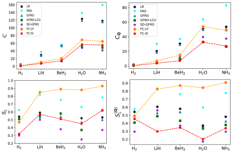
Figure 3: Left panels: $C$ and $S_{L}$ [Eqs. (18) and (19)] descriptors of spectral range distribution of Hamiltonian fragments for different partition methods. As a visual aid, descriptor data associated to qubit methods is highlighted with dashed lines. Right panels: symmetry-projected versions of $C$ and $S_{L}$, $C_{\mathbf{Q}}$ and $S^{(\mathbf{Q})}_{L}$, where the subindex $\mathbf{Q}$ denotes the set of quantum numbers that label the symmetric manifold of the projection.

From Fig. 2, it is evident that Trotter errors are consistently smaller for the greedy approaches compared to the non-greedy counterparts for both fermionic and qubit techniques (cf. FRO with GFRO, and FC-LF with FC-SI). Using greedy approaches and LCU-inspired post processing as well as one- and two-electron combining SD-pre-processing make fermionic techniques more accurate than their qubit counterparts. Further insights on these observations can be drawn with the aid of Fig. 3 , where the $S_{L}$ and $C$ descriptors for the different methods are presented. We can use the latter to understand the large $\alpha$’s corresponding to water and ammonia partitioned with the FRO scheme, and the relatively close Trotter errors for the rest of molecules which lead to a clustering in Fig. 1. The reasons are 1) the larger spectral range of fragments obtained for these molecules and method (see Fig. 3) and 2) the rapid (quadratic) dependence of the error with the sum of these ranges as can be seen in Eq. (19).

We see from Fig. 3 a significant difference in magnitudes of $\beta$ depending on whether the method is fermionic- or qubit-based, but the correlated and monotonic $\alpha-\beta$ relationship is maintained within each family. Therefore, the descriptors $S_{L}$ and $C$ introduced in Eq. (19) should be compared between methods pertaining to the same decomposition technique type (fermionic or qubit-based).

However, it is interesting to note that qubit methods tend to yield smaller $C$ values with respect to most of the fermionic methods. We conjecture that this is due to the less restrictive optimization of fragments compared to fermionic methods, for which spin and particle number symmetries are preserved, whereas that is not the case for qubit methods. In fact, after mapping fermionic Hamiltonian fragments to qubit encodings we notice that the number of Pauli words tend to be significantly larger than the average number of Pauli words of qubit Hamiltonian fragments. These additional number of Pauli words, appear to account for the conservation of symmetries for fermionic Hamiltonian fragments, which ultimately can lead to larger spectral ranges (and $C$ metrics) for the latter. We note from Fig. 3 that greedy algorithms, GFRO, SD-GFRO, and FC-SI exhibit both lower $C$ and $S_{L}$ values with respect to the non-greedy versions (cf. FC-LF with FC-SI). This observation implies that Hamiltonian decomposition methods that favor low and non-uniformly distributed spectral ranges in the resulting Hamiltonian fragments tend to reduce the Trotter error.

On top of the greedy character of Hamiltonian fragments, we show in Fig. 2 that the LCU post-processing can introduce further improvements in Trotter error. From Fig. 3 it is evident that postprocessing endows smaller spectral ranges to the resulting Hamiltonian fragments, reflected in the decrease of both $C$ and $C_{\mathbf{Q}}$.

The only molecule that has not benefited from this procedure is NH₃ for which LCU-post processing increases Trotter error (Fig. 2). This is in contrast with the descriptors $S_{L},C$ and its symmetry-projected versions $C_{\mathbf{Q}},S^{(\mathbf{Q})}_{L}$, that predict a lower Trotter error after LCU post-processing. We attribute this trend violation to the loose character of the descriptors to estimate $\alpha$ and $\alpha_{\mathbf{Q}}$, which fail to quantitatively predict changes in Trotter error after post-processing. Note that tighter Trotter error estimators would be needed especially for NH₃ where the relative change in Trotter error is smaller than the rest of molecules for post-processing.

Interestingly, according to Fig. 3, SD-GFRO is expected to be the best performing fermionic method in terms of Trotter error when considering the non-symmetry projected $C$ and $S_{L}$ descriptors. This is mainly due to the non-uniform spectral range distribution for its Hamiltonian fragments. However, when considering symmetry-projected descriptors, which provide a tighter estimation of the Trotter error, we note that GFRO-LCU becomes competitive, as the latter introduces in some Hamiltonian decompositions either fragments with smaller spectral norms, or a more uneven spectral range distributions with respect to those in SD-GFRO. In fact, similar Trotter errors are observed for both methods, as summarized in Fig. 2.

3.2 Number of single-qubit rotations

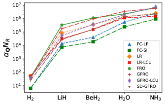
Figure 4: Symmetry-projected Trotter errors (in squared Hartrees) scaled by the number of single qubit rotations in each Trotter step, $N_{R}$, for the Hamiltonian partitions. As highlighted in the main text, this figure of merit gauges the complexity of the circuits required for energy eigenvalue estimation for a Trotterized (Adaptive) QPE algorithm.

Molecule	1st Best ($N_{T}$)	2nd Best ($N_{T}$)	3rd Best ($N_{T}$)
H2	FC-SI (9.45$\times$108)	FC-LF (9.45$\times$108)	SD-GFRO (4.33$\times$109)
LiH	FC-SI (1.94$\times$1012)	FC-LF (3.73$\times$1012)	SD-GFRO (7.73$\times$1012)
BeH2	FC-SI (5.19$\times$1012)	FC-LF (1.16$\times$1013)	LR-LCU ($4.73\times 10^{13}$)
H2O	FC-SI ($7.6\times 10^{13}$)	FC-LF ($1.79\times 10^{14}$)	LR-LCU ($3.82\times 10^{14}$)
NH3	FC-SI ($3.16\times 10^{14}$)	LR-LCU ($5.09\times 10^{14}$)	SD-GFRO ($7.56\times 10^{14}$)

Table 2: Best resource-efficient Hamiltonian decomposition methods for the tested molecules for eigenvalue estimation within a $10^{-3}$ h error with a Trotterized Adaptive QPE algorithm. An upper bound estimation of T-gate count $N_{T}$ is indicated with parenthesis. The latter are calculated according to the procedure outlined in Appendix A.

Figure 4 shows the results for our metric of complexity of circuits required for eigenvalue estimation under a Trotterized Adaptive QPE scheme. Symmetry-projected $\alpha_{\mathbf{Q}}$ is used for a tighter estimation of circuit complexity. Even though fermionic methods have smaller $\alpha_{\mathbf{Q}}$ and $\Gamma$ compared to the qubit-based counterparts, the single rotation gate count $N_{R}$ is lower for the greedy qubit techniques which ultimately yields more resource-efficient circuits for the latter. This can be attributed to two factors: First, the (upper bound for) number of single-qubit rotations for qubit techniques is the same as the number of terms in the Hamiltonian ($\mathcal{O}(N^{4})$), and it does not change with the partitioning. Second, for fermionic fragments the number of single qubit rotation count per fragment scales $\mathcal{O}(N^{2})$, but the number of fragments grows as $\mathcal{O}(N^{2})$ or faster in greedy versions. In addition, prefactors of these dependencies play a decisive role for fixed systems.

Finally, we highlight that in spite of its simplicity, our figure of merit $\alpha_{\mathbf{Q}}N_{R}$ is a good indicator of resource efficiency, as it predicts the best performing methods when we carry out upper-bound T-gate counts ($N_{T}$) that take into account T-gate synthesis approximations and limited phase estimation resolution as sources of error in eigenvalue estimation (see Fig. 4 and Table 2 ). For the range of the $\alpha_{\mathbf{Q}}N_{R}$ metric considered in this work, its fidelity for resource estimation is due to the monotonic character of $N_{T}$ with the former (see Appendix A). It is an open question whether this monotonic dependence is preserved for larger $\alpha_{\mathbf{Q}}N_{R}$ and it is out of the scope of the present work.

4 Conclusions

We have assessed first-order Trotter product formula errors for different partitioning schemes of electronic Hamiltonians.

Taking advantage of Hamiltonian fragment symmetries improves the tightness of Trotter error estimates if the propagated wavefunction is symmetric. Greedy algorithms yield lower Trotter errors than their non-greedy counterparts, which can be rationalized by introducing the upper bound for the Trotter error that uses spectral ranges of individual fragments. This upper bound allowed us to identify two main error contributions: 1) sum over fragment Hamiltonian spectral ranges and 2) linearized entropy factor that favors uneven distributions and explains success of greedy techniques.

These observations are expected to hold for higher-order Trotter formulas, for which it has been proved that the commutator-dependent scaling of Trotter error up to leading order in the simulation time step is [11]:

$$\alpha^{(p)}=\sum_{n_{1},n_{2},\dots,n_{p+1}}^{\Gamma}||[\hat{H}_{n_{p+1}},\cdots[\hat{H}_{n_{2}},\hat{H}_{n_{1}}]\cdots]||$$ (48)

$p$ being the order of the Trotter formula. For instance, one can write the upper bound for the second-order Trotter error as

$$\alpha^{(2)}\leq 2\sum_{n_{1},n_{2},n_{3}}^{\Gamma}||\hat{H}_{n_{1}}||\cdot||[\hat{H}_{n_{2}},\hat{H}_{n_{3}}]||.$$ (49)

To obtain the upper bound for the right hand side we can use the same ideas as in Eq. (19), which give an estimator for the second order Trotter error

$$\alpha^{(2)}\leq\frac{C^{3}S_{L}}{2}.$$ (50)

Hence, we conjecture that decompositions of the Hamiltonian that favors low spectral range Hamiltonian fragments as well as non-uniformity in the distribution of spectral ranges, such as greedy algorithms, are beneficial to the purpose of Trotter error lowering, even beyond the first order Trotter.

On top of the greedy strategy, LCU post-processing of Hamiltonian fermionic fragments can improve Trotter errors even more. However, fermionic decompositions are not the most resource-efficient for Hamiltonian simulation considering the number of single qubit rotations, which is proportional to the number of T-gates expected after compilation into a quantum circuit. Qubit-based decompositions have lower numbers of single-qubit rotations compared to fermionic ones.

We note that scaling of the number of single-qubit rotations as a function of simulated spin-orbitals (qubits) between qubit methods and the most resource-efficient fermionic partitioning (i.e. LR-LCU) is the same, and it goes as $\mathcal{O}(N^{4})$. It is an interesting question to explore whether qubit techniques remain as the most economical in the large $N$ limit. For that end, a better understanding of the scaling of the number of greedy fermionic fragments (which afford the lowest Trotter errors) with the number of simulated spin orbitals as well as the implementation of truncation in the number of fragment schemes, is subject of future study.

Appendix A T-gate count estimations.

Here, we elaborate on upper-bound estimations for T-gate count for a fixed target error $\epsilon$ in energy eigenvalue estimation in a Trotterized Adaptive Quantum Phase Estimation algorithm [39, 9]. The total T-gate count $N_{T}$, as pointed out in previous works [40, 9] is given by

$$N_{T}=N_{R}N_{HT}N_{PE}$$ (51)

where $N_{R}$ is the number of single-qubit rotations needed for the implementation of a single Trotter step in a quantum computer. $N_{HT}$ refers to the number of T gates needed to compile one single qubit rotation (for a fixed target error $\epsilon_{HT}$) and $N_{PE}$ is the number of Trotter steps required to resolve the target energy eigenvalue under a target uncertainty $\epsilon_{PE}$, the latter scaling as $t^{-1}$, $t$ being the total simulation time. The Trotter errors $\alpha,\alpha_{\mathbf{Q}}$ can be shown [9] to define the scaling of an upper bound in the energy eigenvalue estimation error incurred by the Trotter approximation of unitary evolution, and is given by $\epsilon_{T}=\alpha t$. $N_{T}$ can be written in terms of the aforementioned errors as

$$N_{T}\approx\frac{0.76\pi\alpha N_{R}}{|\epsilon_{T}|\epsilon_{PE}}\left[1.15\log_{2}\left(\frac{N_{R}\alpha}{\epsilon_{HT}|\epsilon_{T}|}\right)+9.2\right]$$ (52)

By restricting the target error in eigenvalue estimation to $\epsilon$, we have that $\epsilon=\epsilon_{T}+\epsilon_{HT}+\epsilon_{PE}$. It is generally the case [9] that $\epsilon_{T}>\epsilon_{PE}\gg\epsilon_{HT}$, such that

$$\begin{split}N_{T}&\approx\frac{0.76\pi\alpha N_{R}}{|\epsilon_{T}|(\epsilon-|\epsilon_{T}|)}\\ \times&\left[1.15\log_{2}\left(\frac{N_{R}\alpha}{(\epsilon-\epsilon_{PE}-|\epsilon_{T}|)|\epsilon_{T}|}\right)+9.2\right].\end{split}$$ (53)

Thus, we can optimize over the target errors $|\epsilon_{T}|,\epsilon_{PE}$ to minimize the number of T-gates $N_{T}$. We performed calculations of $N_{T}$ for all methods and molecules addressed in this work and the best performing Hamiltonian decomposition techniques are summarized in Table 2. The reason behind our choice of gauging the complexity of the circuits for each partition method by means of the figure of merit $\alpha_{\mathbf{Q}}N_{R}$ instead of $N_{T}$ (Fig. 4), is the simplicity of the former and highlights the relevance of both the error $\alpha_{\mathbf{Q}}$ as well as the number of Hamiltonian fragments encoded in $N_{R}$ that ensues from the decomposition methods. Indeed this figure of merit exhibits high fidelity in comparing the complexity of circuits among decomposition methods as outlined in the main text.

Appendix B Computational details.

The Hamiltonian fragments for molecules and methods considered in this work, alongside the code used for the calculation of Trotter errors and its analysis can be accessed in a developer version of TEQUILA platform [41] available at https://github.com/lamq317/tequila . For reproduction of Trotter error data, see the script https://github.com/lamq317/tequila/blob/pr-troterr/tests/testTrotErr.py . All Hamiltonian fragments, except for SD-GFRO, were generated using a code based on the Scipy optimize library [42] and the BFGS algorithm [43] for fermionic decomposition methods. SD-GFRO fragments were generated using the code available at https://github.com/iloaiza/MAMBO . The latter can also be used to generate the rest of Hamiltonian fragments considered in this work, using different numerical libraries.

References

- [1] Trygve Helgaker, Poul Jorgensen, and Jeppe Olsen. “Molecular electronic-structure theory”. John Wiley & Sons. (2014).
- [2] Andrew M. Childs, Richard Cleve, Enrico Deotto, Edward Farhi, Sam Gutmann, and Daniel A. Spielman. “Exponential algorithmic speedup by a quantum walk”. In Proceedings of the Thirty-Fifth Annual ACM Symposium on Theory of Computing. Pages 59–68. New York, NY, USA (2003).
- [3] Andrew M Childs. “On the relationship between continuous-and discrete-time quantum walk”. Commun. Math. Phys. 294, 581–603 (2010).
- [4] Guang Hao Low and Isaac L. Chuang. “Hamiltonian simulation by qubitization”. Quantum 3, 163 (2019).
- [5] Andrew M. Childs and Nathan Wiebe. “Hamiltonian simulation using linear combinations of unitary operations”. Quantum Inf. Comput. 12, 901–924 (2012).
- [6] Seth Lloyd. “Universal quantum simulators”. Science 273, 1073–1078 (1996).
- [7] Andrew M. Childs and Yuan Su. “Nearly optimal lattice simulation by product formulas”. Phys. Rev. Lett. 123, 050503 (2019).
- [8] Ryan Babbush, Jarrod McClean, Dave Wecker, Alán Aspuru-Guzik, and Nathan Wiebe. “Chemical basis of trotter-suzuki errors in quantum chemistry simulation”. Physical Review A 91, 022311 (2015).
- [9] Ian D. Kivlichan, Craig Gidney, Dominic W. Berry, Nathan Wiebe, Jarrod McClean, Wei Sun, Zhang Jiang, Nicholas Rubin, Austin Fowler, Alán Aspuru-Guzik, Hartmut Neven, and Ryan Babbush. “Improved fault-tolerant quantum simulation of condensed-phase correlated electrons via trotterization”. Quantum 4, 296 (2020).
- [10] Minh C. Tran, Su-Kuan Chu, Yuan Su, Andrew M. Childs, and Alexey V. Gorshkov. “Destructive error interference in product-formula lattice simulation”. Phys. Rev. Lett. 124, 220502 (2020).
- [11] Andrew M. Childs, Yuan Su, Minh C. Tran, Nathan Wiebe, and Shuchen Zhu. “Theory of trotter error with commutator scaling”. Phys. Rev. X 11, 011020 (2021).
- [12] Conor Mc Keever and Michael Lubasch. “Classically optimized hamiltonian simulation”. Phys. rev. res. 5, 023146 (2023).
- [13] Abhinav Kandala, Antonio Mezzacapo, Kristan Temme, Maika Takita, Markus Brink, Jerry M. Chow, and Jay M. Gambetta. “Hardware-efficient variational quantum eigensolver for small molecules and quantum magnets”. Nature 549, 242–246 (2017).
- [14] Yuta Matsuzawa and Yuki Kurashige. “Jastrow-type decomposition in quantum chemistry for low-depth quantum circuits”. J. Chem. Theory Comput. 16, 944–952 (2020).
- [15] Vladyslav Verteletskyi, Tzu-Ching Yen, and Artur F. Izmaylov. “Measurement optimization in the variational quantum eigensolver using a minimum clique cover”. J. Chem. Phys. 152, 124114 (2020).
- [16] Tzu-Ching Yen, Vladyslav Verteletskyi, and Artur F. Izmaylov. “Measuring all compatible operators in one series of single-qubit measurements using unitary transformations”. J. Chem. Theory Comput. 16, 2400–2409 (2020).
- [17] Mario Motta, Erika Ye, Jarrod R. McClean, Zhendong Li, Austin J. Minnich, Ryan Babbush, and Garnet Kin-Lic Chan. “Low rank representations for quantum simulation of electronic structure”. NPJ Quantum Inf. 7, 1–7 (2021).
- [18] Tzu-Ching Yen and Artur F. Izmaylov. “Cartan subalgebra approach to efficient measurements of quantum observables”. PRX Quantum 2, 040320 (2021).
- [19] Alberto Peruzzo, Jarrod McClean, Peter Shadbolt, Man-Hong Yung, Xiao-Qi Zhou, Peter J. Love, Alán Aspuru-Guzik, and Jeremy L. O’Brien. “A variational eigenvalue solver on a photonic quantum processor”. Nat. Commun. 5, 1–7 (2014).
- [20] Ewout van den Berg and Kristan Temme. “Circuit optimization of hamiltonian simulation by simultaneous diagonalization of pauli clusters”. Quantum 4, 322 (2020).
- [21] Michael A. Nielsen and Isaac L. Chuang. “Quantum computation and quantum information”. Cambridge University Press. (2010).
- [22] Craig Gidney and Austin G Fowler. “Efficient magic state factories with a catalyzed to transformation”. Quantum 3, 135 (2019).
- [23] Masuo Suzuki. “General theory of fractal path integrals with applications to many-body theories and statistical physics”. J. Math. Phys. 32, 400–407 (1991).
- [24] Ignacio Loaiza, Alireza Marefat Khah, Nathan Wiebe, and Artur F Izmaylov. “Reducing molecular electronic hamiltonian simulation cost for linear combination of unitaries approaches”. Quantum Sci. Technol. 8, 035019 (2023).
- [25] David Layden. “First-order trotter error from a second-order perspective”. Phys. Rev. Lett. 128, 210501 (2022).
- [26] Vlad Gheorghiu, Michele Mosca, and Priyanka Mukhopadhyay. “A (quasi-) polynomial time heuristic algorithm for synthesizing t-depth optimal circuits”. Npj Quantum Inf. 8, 1–11 (2022).
- [27] Priyanka Mukhopadhyay, Nathan Wiebe, and Hong Tao Zhang. “Synthesizing efficient circuits for hamiltonian simulation”. npj Quantum Information 9, 31 (2023).
- [28] Jacob T Seeley, Martin J Richard, and Peter J Love. “The bravyi-kitaev transformation for quantum computation of electronic structure”. J. Chem. Phys. 137, 224109 (2012).
- [29] Artur F Izmaylov and Tzu-Ching Yen. “How to define quantum mean-field solvable hamiltonians using lie algebras”. Quantum Science and Technology 6, 044006 (2021).
- [30] Seonghoon Choi, Ignacio Loaiza, and Artur F Izmaylov. “Fluid fermionic fragments for optimizing quantum measurements of electronic hamiltonians in the variational quantum eigensolver”. Quantum 7, 889 (2023).
- [31] Joonho Lee, Dominic W Berry, Craig Gidney, William J Huggins, Jarrod R McClean, Nathan Wiebe, and Ryan Babbush. “Even more efficient quantum computations of chemistry through tensor hypercontraction”. PRX Quantum 2, 030305 (2021).
- [32] P. Jordan and E. Wigner. “Über das paulische Äquivalenzverbot.”. Z. Physik 47, 631–651 (1928).
- [33] Sergey B. Bravyi and Alexei Yu Kitaev. “Fermionic quantum computation”. Ann. Phys. 298, 210–226 (2002).
- [34] Zachary Pierce Bansingh, Tzu-Ching Yen, Peter D Johnson, and Artur F Izmaylov. “Fidelity overhead for nonlocal measurements in variational quantum algorithms”. J. Phys. Chem. A 126, 7007–7012 (2022).
- [35] Ophelia Crawford, Barnaby van Straaten, Daochen Wang, Thomas Parks, Earl Campbell, and Stephen Brierley. “Efficient quantum measurement of pauli operators in the presence of finite sampling error”. Quantum 5, 385 (2021).
- [36] Yuan Su, Hsin-Yuan Huang, and Earl T. Campbell. “Nearly tight trotterization of interacting electrons”. Quantum 5, 495 (2021).
- [37] S. Bravyi, J.M. Gambetta, A. Mezzacapo, and K Temme. “Tapering off qubits to simulate fermionic hamiltonians.” (2017). arXiv:1701.08213.
- [38] Jarrod R. McClean, Nicholas C. Rubin, Kevin J. Sung, Ian D. Kivlichan, Xavier Bonet-Monroig, Yudong Cao, Chengyu Dai, E. Schuyler Fried, Craig Gidney, Brendan Gimby, et al. “Openfermion: the electronic structure package for quantum computers”. Quantum Sci. Technol. 5, 034014 (2020).
- [39] Dominic W. Berry, Brendon L. Higgins, Stephen D. Bartlett, Morgan W. Mitchell, Geoff J. Pryde, and Howard M. Wiseman. “How to perform the most accurate possible phase measurements”. Phys. Rev. A 80, 052114 (2009).
- [40] Markus Reiher, Nathan Wiebe, Krysta M. Svore, Dave Wecker, and Matthias Troyer. “Elucidating reaction mechanisms on quantum computers”. Proc. Natl. Acad. Sci. U.S.A. 114, 7555–7560 (2017).
- [41] Jakob S Kottmann, Sumner Alperin-Lea, Teresa Tamayo-Mendoza, Alba Cervera-Lierta, Cyrille Lavigne, Tzu-Ching Yen, Vladyslav Verteletskyi, Philipp Schleich, Abhinav Anand, Matthias Degroote, et al. “Tequila: A platform for rapid development of quantum algorithms”. Quantum Sci. Technol. 6, 024009 (2021).
- [42] Pauli Virtanen, Ralf Gommers, Travis E. Oliphant, Matt Haberland, Tyler Reddy, David Cournapeau, Evgeni Burovski, Pearu Peterson, Warren Weckesser, Jonathan Bright, Stéfan J. van der Walt, Matthew Brett, Joshua Wilson, K. Jarrod Millman, Nikolay Mayorov, Andrew R. J. Nelson, Eric Jones, Robert Kern, Eric Larson, C J Carey, İlhan Polat, Yu Feng, Eric W. Moore, Jake VanderPlas, Denis Laxalde, Josef Perktold, Robert Cimrman, Ian Henriksen, E. A. Quintero, Charles R. Harris, Anne M. Archibald, Antônio H. Ribeiro, Fabian Pedregosa, Paul van Mulbregt, and SciPy 1.0 Contributors. “SciPy 1.0: Fundamental Algorithms for Scientific Computing in Python”. Nat. Methods 17, 261–272 (2020).
- [43] Roger Fletcher. “Practical methods of optimization”. John Wiley & Sons. (2013).