Inflationary and phase-transitional primordial magnetic fields in galaxy clusters

Abstract

Primordial magnetic fields (PMFs) are possible candidates for explaining the observed magnetic fields in galaxy clusters. Two competing scenarios of primordial magnetogenesis have been discussed in the literature: inflationary and phase-transitional. We study the amplification of both large- and small-scale correlated magnetic fields, corresponding to inflation- and phase transition-generated PMFs, in a massive galaxy cluster. We employ high-resolution magnetohydrodynamic cosmological zoom-in simulations to resolve the turbulent motions in the intracluster medium. We find that the turbulent amplification is more efficient for the large-scale inflationary models, while the phase transition-generated seed fields show moderate growth. The differences between the models are imprinted on the spectral characteristics of the field (such as the amplitude and the shape of the magnetic power spectrum) and therefore on the final correlation length. We find a one order of magnitude difference between the final strengths of the inflation- and phase transition-generated magnetic fields, and a factor of $1.5$ difference between their final coherence scales. Thus, the final configuration of the magnetic field retains information about the PMF generation scenarios. Our findings have implications for future extragalactic Faraday rotation surveys with the possibility of distinguishing between different magnetogenesis scenarios.

1 Introduction

Galaxy clusters, the largest virialized structures of the universe, reveal the existence of large-scale correlated magnetic fields in the dilute plasma between galaxies that is known as the intracluster medium (ICM). Studies of Faraday rotation measures, as well as diffuse radio emissions in the form of radio halos and radio relics, have probed the strength and morphology of the ICM magnetic field (see, e.g., Govoni & Feretti, 2004; Brüggen et al., 2012; van Weeren et al., 2019, for reviews). These different observational methods infer a field strength of the order of microGauss and coherence scales reaching a few tens of kiloparsecs in galaxy clusters (see, e.g., Govoni & Feretti, 2004; van Weeren et al., 2019).

Despite their ubiquity, the origins of cluster magnetic fields remain elusive. A commonly accepted hypothesis is that weak seed magnetic fields, generated from an initially zero magnetic field (Rees, 1987), are amplified during structure formation via the combined effects of adiabatic compression and a small-scale dynamo (see, e.g., the recent review by Donnert et al., 2018). It is debatable whether these seed magnetic fields are produced in the early universe by the primordial magnetogenesis or whether they are produced at a later epoch, during structure formation, by astrophysical mechanisms (e.g., the Biermann battery mechanism and the Weibel instability— Biermann, 1950; Lazar et al., 2009). In the primordial scenario, magnetic fields originating in the early universe, i.e., primordial magnetic Fields (PMFs), have volume-filling fractions that are close to unity, making them good candidates for explaining the magnetization of cosmic voids. This scenario is favored by observations of blazar spectra that rule out the possibility of a zero magnetic field in the intergalactic medium (IGM; see Ackermann et al., 2018, and references therein). On the other hand, the astrophysical scenario requires efficient transport mechanisms of magnetic energy toward larger scales, to explain the possible magnetization of cosmic voids. Galactic winds (Kronberg et al., 1999; Bertone et al., 2006) as well as jets and lobes from radio galaxies (Daly & Loeb, 1990) have been proposed as such efficient transport processes. However, the significance of the volume-filling factor of such a locally generated and transported magnetic field remains unclear (see, e.g., Dolag et al., 2011; Bondarenko et al., 2022).

PMFs could result from different magnetogenesis scenarios. Their post-recombination magnetic structure and the field coherence scale depend on: (1) the details of the particular magnetogenesis model; and (2) evolutionary trends in the pre-recombination universe. A primordial seed field could be generated during inflation or phase transitions (see Subramanian, 2016; Vachaspati, 2021, for recent reviews). In inflationary magnetogenesis, the coherence scale of the quantum-mechanically produced seed magnetic field can be stretched on superhorizon scales. However, the conformal invariance of the electromagnetic action must be broken (see, e.g., Dolgov, 1993) in order to achieve sufficiently strong seed fields for their subsequent growth at later epochs. This is usually ensured by the coupling of the electromagnetic action with scalar fields, such as the inflaton (Turner & Widrow, 1988; Ratra, 1992), or by nonminimal coupling with the scalar-tensor gravity, as has been proposed by Mukohyama (2016). Contrary to the inflationary scenario, the coherence scale of the phase transition-generated field is limited by the Hubble horizon scale, and it is a sizeable fraction of the Hubble scale. The electroweak (EW) or quantum-chromodynamical (QCD) phase transitions produce seed fields through nonequilibrium processes, e.g., during the collision (Ahonen & Enqvist, 1998; Copeland et al., 2000) and nucleation (Cheng & Olinto, 1994; Sigl et al., 1997) of bubbles of different phases (see Kandus et al., 2011, for a review). Both inflation- and phase transition-generated seed fields are assumed to have a stochastic distribution. In addition, in the inflationary scenario, the constant, spatially uniform magnetic field is predicted by the Mukohyama model (Mukohyama, 2016; Brandenburg et al., 2020).

The evolution of PMFs proceeds as “freely decaying turbulence” in the radiation-dominated epoch (see, e.g., Brandenburg et al., 1996; Christensson et al., 2001; Banerjee & Jedamzik, 2004; Kahniashvili et al., 2016; Brandenburg et al., 2018). The correlation length of the small-scale (phase-transitional) as well as the large-scale (inflationary) correlated primordial field increases, although much more efficiently in the former case, due to an inverse cascade (Kahniashvili et al., 2010; Brandenburg et al., 2018). The field is expected to freeze and retain its characteristic spectral profile, from the moment of recombination until reionization. The formation of massive structures, such as galaxy clusters, and the subsequent amplification of PMFs on the corresponding scales (see Donnert et al., 2018, for a review), can be studied with cosmological magnetohydrodynamic (MHD) simulations (see, e.g., Dolag et al., 1999; Dubois & Teyssier, 2008; Xu et al., 2009; Vazza et al., 2014; Marinacci et al., 2018). In the present paper, we study the amplification of the two types of PMFs in a massive galaxy cluster with the Enzo code (Bryan et al., 2014), using the adaptive mesh refinement (AMR) technique. For the first time, we compare the evolution of small- and large-scale correlated PMFs, consistent with different inflationary and phase-transitional primordial magnetogenesis scenarios.

The structure of this paper is as follows. In Section 2 we discuss our physical model and our motivation for studying different PMFs. In Section 3, we describe our numerical setup, the initial conditions, and the details of the simulated galaxy cluster. In Section 4, we present our results. Finally, we discuss possible numerical caveats in Section 5 and we summarize our main results in Section 6.

2 Physical model

In this section, we describe the spectral characteristics of the inflation- and phase transition-generated PMFs that are used as initial conditions in our simulations. Regardless of the magnetogenesis scenario, it is generally expected that after generation, the primordial seed magnetic field is frozen in, and the amplitude of the (physical) magnetic field decreases with the expansion of the universe, $B_{\text{phys}}\propto 1/a^{2}$; equivalently, magnetic field lines are adiabatically stretched, with a $\propto\rho_{\text{phys}}^{2/3}$ scaling, where $\rho_{\text{phys}}$ is the gas density. This treatment of the magnetic field may be justified in a highly conducting fluid, such as the hot plasma in the early universe, if there is no turbulence. However, the concept of simple adiabatic dilution has to be abandoned, when the effects of turbulence can become important. Turbulent magnetic fields could be generated either at the end of inflation through the inflaton decay to standard model fields, or during phase transitions, through collisions between the expanding bubbles of the new phase (see Subramanian, 2016; Vachaspati, 2021, for reviews), and they could alter the evolution of different primordial seed magnetic fields. Random magnetic fields could also be generated when the phase transition only involves a smooth crossover to the new phase, without bubbles. In the following, we will discuss how the statistical properties of the inflation- and phase transition-generated magnetic fields are modified when taking into account their turbulent (pre-recombination) evolution after their generation.

In the statistical framework, the description of PMFs relies on the definition of the magnetic energy power spectra and their characteristic length scales (also see the discussion in Section 3 of Mtchedlidze et al., 2022, hereafter, Paper I). The magnetic energy power spectrum $E_{B}(k)$ is often conveniently split into its large-scale, $E_{B}^{\text{LS}}$ and small-scale, $E_{B}^{\text{SS}}$ parts. The transition from the large-scale to the small-scale spectra occurs at the scale corresponding to the wavenumber $k_{\rm peak}$. In the case of phase transition-generated PMF, this scale corresponds to the phase transition bubble size and cannot exceed the Hubble horizon size at the moment of field generation (see, e.g., Kahniashvili et al., 2010). After their generation, the decaying turbulence leads to a magnetic energy spectrum, which can either be $E_{B}^{\text{LS}}\propto k^{2}$, commonly known as the “Saffman spectrum” (Hogan, 1983), or $E_{B}^{\text{LS}}\propto k^{4}$, known as the “Batchelor spectrum” (Davidson, 2015). As Kahniashvili et al. (2010) have shown, the realization of these spectra depends on the driving nature of the turbulent magnetic field. If the turbulence is driven through kinetic energy injection, magnetic field develops a spectrum close to $E_{B}^{\text{LS}}\propto k^{4}$ (Batchelor) spectrum; if the initial driver is a magnetic field, then the spectrum is shallower than $E_{B}^{\text{LS}}\propto k^{3}$. In addition, the recent work of Brandenburg et al. (2023b) has shown that in the former scenario (weak magnetic fields), the Batchelor and Saffman spectra result from small-scale dynamo action, in its kinematic and saturated states, respectively. The Batchelor spectrum is also expected from the causality condition being combined with the divergence-free field condition (Durrer & Caprini, 2003). Finally, on smaller scales, a turbulent magnetic cascade with $E_{B}^{\text{SS}}\propto k^{-5/3}$ is expected for both the Saffman and Batchelor spectra.

The inflationary scenario, in turn, predicts a magnetic energy spectrum that can be nearly scale-invariant at the moment of generation, i.e., $E_{B}(k)\propto k^{-1}$. This scaling is further modified, due to turbulent decay during the pre-recombination epoch, and results in a Kolmogorov $k^{-5/3}$ spectrum by the end of recombination (Kahniashvili et al., 2017). It should be noted that a transition to the $k^{4}$ spectrum (IR cutoff) could also be a possible outcome of inflation, although on much larger scales than the characteristic scale for the phase-transitional scenarios, that is, $k_{\rm peak}^{\rm infl}\ll k_{\rm peak}^{\rm PT}$ (see, e.g., Brandenburg et al., 2018). In this case, Brandenburg et al. (2018) found that for a certain wavenumber range (close to the peak of the spectrum, $k>k_{\rm peak}^{\rm infl}$), the power spectrum will still be characterized by the scale-invariant spectrum.

In the present work, we explore two phase transition-generated PMFs that are characterized by a Saffman spectrum and a Batchelor spectrum, respectively, and two inflationary-generated PMFs that are characterized by a turbulent spectrum and by a Dirac delta function (in Fourier space, corresponding to a uniform magnetic field), respectively. The latter model serves as a comparison to our simulations with other cosmological simulations, where a uniform seed magnetic field is commonly assumed as an initial condition (see, e.g., Dolag et al., 2002; Marinacci et al., 2015; Vazza et al., 2018). Nevertheless, the physical generation of a uniform seed magnetic field in the early universe has been predicted to be plausible under specific conditions by Mukohyama (2016). Hereafter, we refer to this model as the Mukohyama model and we also refer the reader to Brandenburg et al. (2020), and the references therein, for more details.

We adopt these models as our initial magnetic conditions, despite our relatively low initial resolution of $312.5\,\,h^{-1}{\rm ckpc}$, where the ‘c’ is commonly used to emphasize comoving units. We note that this initial resolution may not be enough to resolve the magnetic field coherence scales that are expected from theory or the small scales that are dominated by the turbulent spectra. For example, in the phase-transitional scenario, an optimistic assumption of the largest magnetic eddy size would lead to magnetic field coherence scales of the order of $10$ kpc (comoving) at the end of recombination (see, e.g., the constraint plot, Figure 7, in Roper Pol et al., 2022). However, Kahniashvili et al. (2022) have recently proposed that QCD phase transition-generated PMFs could even reach $\sim 300\,{\rm ckpc}$ coherence scales (if the field is fully helical), by accounting for the decaying nature of turbulent sources between the time of generation and big bang nucleosynthesis. The hypothesis behind this finding is that the magnetic correlation length can be larger if one applies the Big Bang nucleosynthesis (BBN) limits not to the time of generation of the seed field, but to the later time of the BBN. While the predicted magnetic field coherence scale may vary from theory to theory, we emphasize that our initial resolution prevents us from having a one-to-one match with any of the various theoretical expectations. It is therefore important to stress that, similar to Paper I, our initial stochastic spectra are only intended to emulate the shapes that are theoretically expected.

3 Simulations

We simulate the formation of a galaxy cluster with the cosmological Eulerian MHD code Enzo (Bryan et al., 2014). We assume a Lambda cold dark matter ($\Lambda$CDM) cosmology ($h=0.674$, $\Omega_{m}=0.315$, $\Omega_{b}=0.0493$, $\Omega_{\Lambda}=0.685$, and $\sigma_{8}=0.807$, as in the Planck Collaboration et al. 2020). As in our previous work (Paper I), we use the Dedner formulation of the MHD equations, to obey the divergence-free condition of the magnetic field (Dedner et al., 2002). In the present paper, we additionally employ AMR to reach a higher resolution within our simulated galaxy cluster (Brummel-Smith et al., 2019).

We follow two steps to solve the galaxy cluster: (1) a global AMR simulation, where we identify a list of fairly resolved haloes and (2) a local AMR or “zoom-in” simulation, where we apply several levels of AMR in a selected region in which the cluster forms. In both setups, the refinement is triggered according to the baryon, $f_{\text{b}}$, and dark matter (DM), $f_{\text{DM}}$, overdensity thresholds. These parameters ensure refinement when the gas (DM) mass in a cell reaches a factor of $f_{\text{b}}$ ($f_{\text{DM}}$) times the mean baryonic (DM) mass expected in a cell at the root grid level (Bryan et al., 2014). In this study, we use a nominal refinement factor of 2 between the parent grid and its subgrid, which is the commonly used value for cosmological simulations (see Bryan et al., 2014, for more details). In the global AMR simulations, we set $f_{\text{b}}=f_{\text{DM}}=4$ and we use 4 levels of refinement that are activated in the whole $(80\,\,h^{-1}{\rm cMpc})^{3}$ simulation box. We use a root grid of $256^{3}$ cells and $256^{3}$ DM particles each of mass $m_{\text{DM}}=3.34\times 10^{9}M_{\odot}$. The initial and final spatial resolutions are $312.5\,\,h^{-1}{\rm ckpc}$ and final $19.5\,\,h^{-1}{\rm ckpc}$, respectively. Based on this simulation, we produce a halo catalog using the yt halo finder (Skory et al., 2011). The halo finder identifies groups of linked DM particles, based on the Eisenstein & Hut (1998) algorithm. The galaxy cluster selected for the present work is among the most massive clusters from our halo catalog (see Section 3.2 for a detail description of the cluster). Next, we resimulate the selected galaxy cluster in the $(80\,\,h^{-1}{\rm cMpc})^{3}$ simulation box, by centering our simulation box where the galaxy cluster forms. We select a volume of $(20\,\,h^{-1}{\rm cMpc})^{3}$ and use seven levels of refinement. In this case, the refinement is triggered on the $f_{\text{b}}=0.1$ and $f_{\text{DM}}=4$ refinement factors, giving us a final maximum spatial resolution of $2.44\,\,h^{-1}{\rm ckpc}$.

Table 1: Initial conditions for the magnetic field. The correlation length and the mean value of the smoothed (on a $1\,h^{-1}{\rm cMpc}$ scale) magnetic field are denoted by $\lambda_{B}$ and $B_{1\rm Mpc}$, respectively, while $\langle B_{0}^{2}\rangle$ and $\langle B_{0}\rangle$ are the means of the initial magnetic field energy and the initial magnetic field strength, respectively.

Scenario	Model	Simulation ID	$\langle B_{0}^{2}\rangle$	$\langle B_{0}\rangle$	$B_{1\rm Mpc}$	$\lambda_{B}$
			[(nG)2]	[nG]	[nG]	[$h^{-1}\,{\rm cMpc}$]
Inflationary	(i) Uniform	u	0.99	0.99	—	—
	(ii) Scale-invariant	km1	0.99	0.92	0.92	33.04
Phase-transitional	(iii) Saffman	k2	0.99	0.92	0.92	1.07
	(iv) Batchelor	k4	0.99	0.92	0.92	0.85

The selection of the overdensity factors, $f_{i}$ (where “i” indicates baryons or DM), is important, and it depends on the problem being addressed. In this work, the grid refinement thresholds are chosen in order to solve the turbulent motions in the ICM that are crucial for the seed magnetic field amplification. Mergers and accretion events that are driven by gravitational dynamics are the main agents of turbulence in the ICM. Therefore, low overdensity thresholds for both gas and DM ensure resolving low-mass gas substructures and DM halos (as discussed in O’Shea et al., 2005), and, thus, the maintenance of turbulence in the ICM (Iapichino & Niemeyer, 2008). Note that lower refinement factors significantly increase the number of refined grids, so one has to compromise between the final resolution and the computational cost. For this purpose, we use a higher value of $f_{\text{DM}}$ compared to the $f_{\text{b}}$ factor. This selection closely follows Vazza et al. (2018), where the authors have proven that the impact of an increased DM resolution on the final magnetic field distribution is only minor (see Figure 17 of Vazza et al., 2018). Indeed, we will show in Section 3.2 that the chosen refinement thresholds result in large turbulence-filling factors in our simulated ICM.

Finally, our simulations do not include gas cooling, chemical evolution, star formation, or feedback from active galactic nuclei. As in Paper I, we focus solely on the magnetic field amplification that is due to structure formation and turbulent flows in the ICM.

3.1 Initial conditions

We study four different realizations of the simulated galaxy cluster. Our simulations differ in the initial magnetic field configurations. We assume only nonhelical magnetic fields at the initial redshift $z=50$. Similar to Paper I, we choose to normalize our initial magnetic conditions, so that they have the same total magnetic energy (see Table 1). The four models are:

1. Uniform (spatially homogeneous) field: a seed magnetic field with a constant strength across the whole computational domain, and directed along the diagonal. This case corresponds to a particular inflationary magnetogenesis scenario—namely, the Mukohyama model (Mukohyama, 2016).

2. Scale-invariant field: this is a setup for a stochastic, statistically homogeneous PMF, corresponding to an inflationary scenario.

3. Saffman model: a stochastic, phase transition-generated PMF, which has a Saffman spectrum, i.e., with a power-law index of 2.

4. Batchelor model: the same stochastic setup as in (3), but with a Batchelor spectrum, i.e., with a power-law index of 4.

The initial conditions (2)–(4) were produced with the Pencil Code (Pencil Code Collaboration et al., 2021). The initial magnetic power spectra for these stochastic setups are shown in Figure 1.

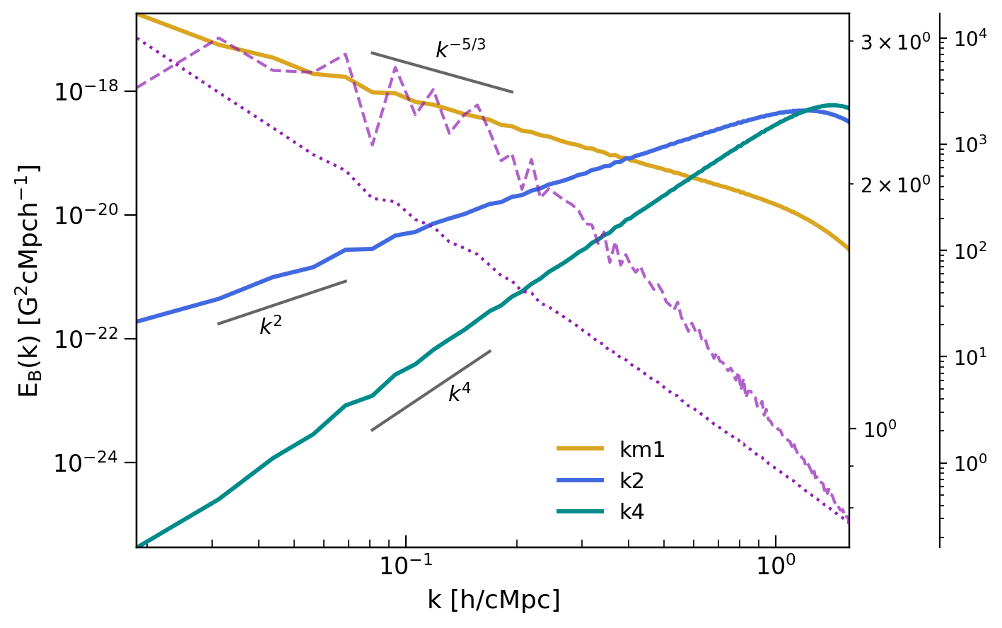
Figure 1: The initial magnetic power spectra for the stochastic setups, with the velocity (dotted purple line) and density (dashed purple line) spectra being shown for the run with the uniform model. The main and second secondary axes shown on the right correspond to the density and velocity spectra, in $(10^{63}\,{\rm g}/\,{\rm cm}^{3})^{2}\,h^{-1}{\rm cMpc}$ and $10^{8}\,{\rm cm}^{2}/\,{\rm s}^{2}\,h^{-1}{\rm cMpc}$ units, respectively. The initial power spectra of the baryon and DM perturbations are nearly indistinguishable at the scales resolved by our resolution. The only difference between these two spectra is in their amplitudes.

We follow the same method as in Paper I to generate our initial conditions. This initial simulation allows us to evolve an initially Gaussian random field, with the desired spectral properties, until the phase of the magnetic field in Fourier space become correlated, and their distribution is no longer one of white noise. This is then used as the actual initial condition for the Enzo simulations. The reader may refer to Appendix A of Paper I for further details concerning the generation and normalization of the initial magnetic conditions (2)–(4).

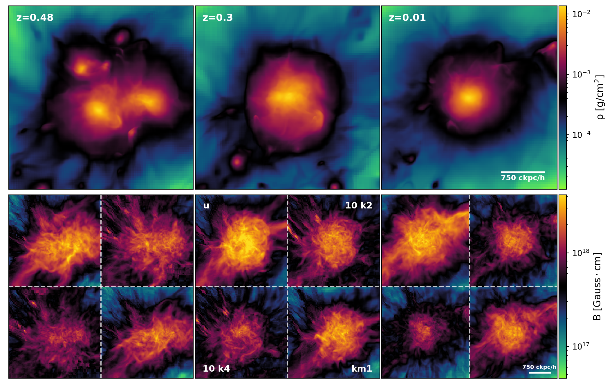
Figure 2: Projected maps of the gas density (top panel) and the magnetic field from a $(3\,h^{-1}{\rm cMpc})^{3}$ box for different seeding scenarios (bottom panel), at different stages of the cluster evolution. The left, middle, and right panels show the projected fields at the merging ($z=0.48$), post-merger ($z=0.3$) and relaxing ($z=0.01$) states, respectively. The magnetic field projections for the Batchelor and Saffman models are normalized by a factor of 10.

We use an initial matter power spectrum, resulting from a primordial, scale-invariant spectrum, by taking into account the evolution of post-inflationary linear perturbations, i.e., we use the transfer function of Eisenstein & Hu (1998). It should be noted that the adopted matter power spectrum neglects any contribution from PMFs. PMFs are expected to affect the clustering of matter on intermediate and small scales, i.e., smaller than galaxy cluster scales (Sethi & Subramanian, 2005; Yamazaki et al., 2006; Fedeli & Moscardini, 2012; Kahniashvili et al., 2013; Sanati et al., 2020, and see also discussion in Paper I). Therefore, we do not expect that the presence of PMF-induced density perturbations in the early universe to have a significant impact on our results.

3.2 Selected cluster

The selected cluster from our two-step simulations can be seen in Figure 2. The total mass of our cluster, $2.39\cdot 10^{14}M_{\odot}$, is comparable to the masses of some observed galaxy clusters, such as A3527 (see, e.g., de Gasperin et al., 2017) or the recently studied Ant cluster (Botteon et al., 2021). We summarize the most important parameters of our simulated cluster in Table 2.

Table 2: Characteristics: mass and energy ratio $E_{\text{kin}}/E_{\text{tot}}$ of the cluster at $z=0$, where $E_{\text{tot}}=E_{\text{kin}}+E_{\text{th}}$.

Radius	Mass	$E_{\text{kin}}/E_{\text{tot}}$
$[\,h^{-1}{\rm cMpc}]$	[$10^{14}M_{\odot}$]
$R_{500}=0.50$	$1.14$	$0.15$
$R_{100}=1.01$	$1.86$	$0.16$
$R_{\text{vir}}=1.54$	$2.39$	$0.16$

The formation history of a galaxy cluster fully determines the amount of amplification of the seed magnetic field. Our selected cluster undergoes a series of mergers, and its evolution can be characterized by three phases: (1) at the early stage of formation, $z\lesssim 0.7$, it continuously grows, by several accreting minor merger events; (2) in the redshift range 0.7 – 0.3, a major merger takes place, with a mass ratio of $1.2$ between the main and secondary clusters (within $R_{500}$ radius), and (3) at late redshifts, i.e., $z<0.3$, it enters into a relaxing state. In Figure 3, we show the mass accretion history of the cluster in the redshift range $1.5>z>0$. The mass of the cluster is computed within $R_{\text{vir}}$, and we show its evolution for the uniform model. We indicate the major merger phase with the shaded gray area ($\sim 2\,{\rm Gyr}$ timescale) in Figure 3.

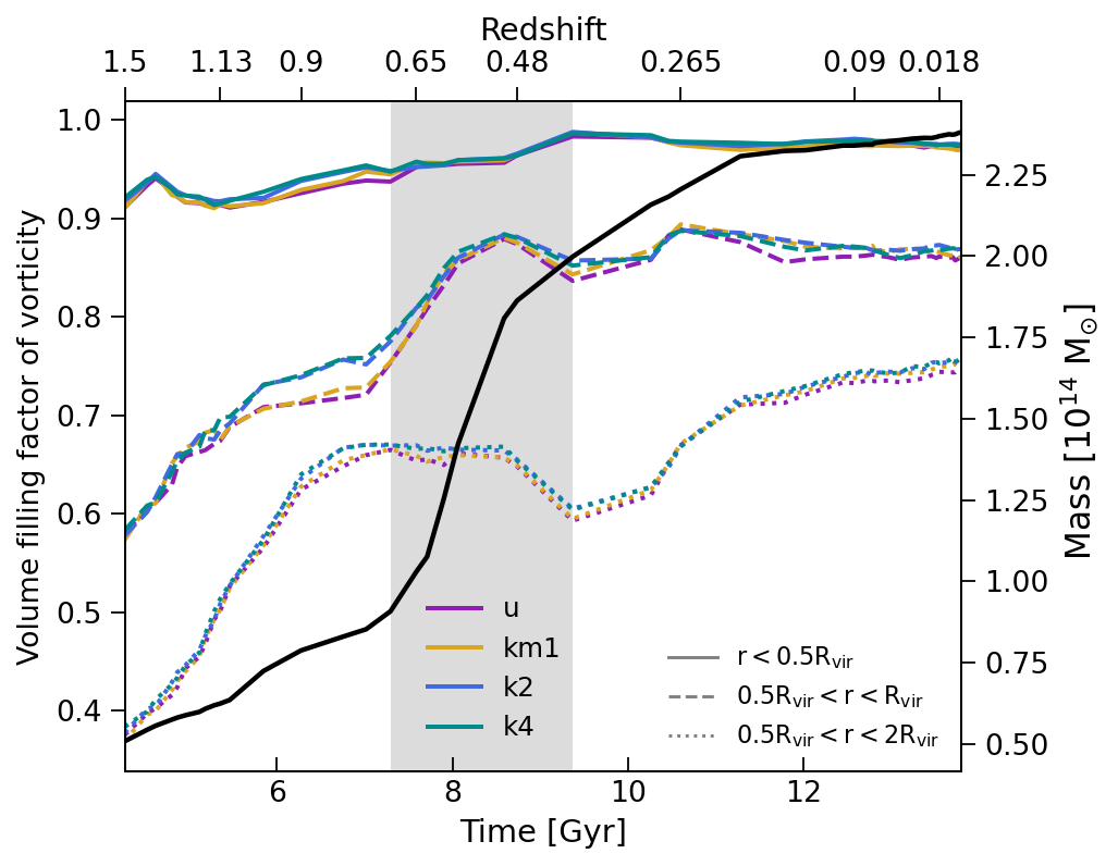
Figure 3: Time evolution of the total virial ($r=R_{\text{vir}}$) mass (black solid line) and vorticity volume-filling factor for the cluster core (solid lines) and the outskirts enclosing a spherical shells in: $0.5\,R_{\text{vir}}<r<R_{\text{vir}}$ (dashed lines) and $0.5\,R_{\text{vir}}<r<2\,R_{\text{vir}}$ (dotted lines).

During this phase, we observe a steep growth of the total mass, which increases by a factor of $\sim 2$.

Mergers of clusters play a key role in shaping the properties of the ICM, by injecting turbulence. To characterize the turbulence in our simulated galaxy cluster, we follow the recipe proposed by Iapichino et al. (2017). In that work, the authors used the vorticity modulus as an indicator of the velocity fluctuations and its volume-filling factor $f_{\omega}$ as a proxy for the turbulent states of galaxy clusters. In detail, the procedure consists of flagging a cell as “turbulent” if it satisfies the criterion (see Kang et al., 2007; Iapichino et al., 2017, and references therein)

$$\omega_{i}>N/t_{\text{age}},$$ (1)

where $\omega_{i}$ is the vorticity in the $i$th cell, $t_{\text{age}}$ is the age of the universe at redshift $z$, and $N$ is the number of eddy turnovers, respectively. Following Iapichino et al. (2017), we set $N=10$. Finally, the volume-filling factor $f_{\omega}$ is the volume fraction satisfying Equation (1). The authors find that $f_{\omega}$ is substantial, both in the core and at the outskirts of their simulated galaxy cluster, reaching $f_{\omega}>90\%$ and $f_{\omega}>60\%$, respectively. In the bottom panel of Figure 3, we show the evolution of the volume-filling factors computed for the core and outskirt regions of our simulated galaxy cluster. The volume-filling factors are also shown to be substantial, with percentages larger than $90\%$ in the core region and $60\%$ in the outskirts. We note that we obtain similar results to Iapichino et al. (2017), even though our numerical setups differ. For example, their simulations use 8 AMR levels, triggered by spatial derivatives of the velocity field, to reach a final maximal resolution of $7.8\,h^{-1}{\rm cMpc}$. Additionally, they make use of a subgrid-scale model, which is based on the Germano (1992) formalism, to account for unresolved turbulent motions in the ICM; see also Schmidt et al. (2006). Thus, our volume-filling factors, along with high final resolution of $2.44\,h^{-1}{\rm ckpc}$, show that our numerical setup is adequate for capturing turbulent motions in the simulated galaxy cluster.

4 Results

4.1 General properties

We start our analysis by giving a qualitative view of the density and magnetic field distribution in the simulated galaxy cluster. In Figure 2, we show the projected density and corresponding magnetic field distribution for different seeding scenarios. The projections are extracted from a $(3\,h^{-1}{\rm cMpc})^{3}$ simulation box, for three different epochs: the merging ($z=0.48$), post-merging ($z=0.3$), and relaxing ($z=0.01$) phases. As we further discuss below, a different initial magnetic structure leads to a different final strength in the simulated galaxy cluster. In order to better visualize the spatial differences between our models in the projected magnetic field distribution, we normalize in Figure 2 the distributions for the Batchelor and Saffman models by a factor of 10. These two models, being initially correlated on smaller scales, already reach the lowest magnetic field strengths at early redshifts, $z\sim 10$ (before the cluster forms), and, later on, at all stages of the cluster evolution.

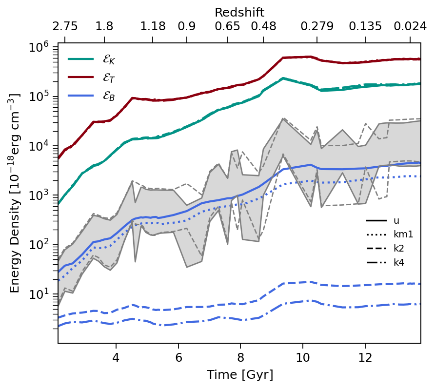
Figure 4: Evolutions of the thermal, kinetic, turbulent kinetic, and magnetic energy densities, obtained from a comoving box with a side length of $1.5\,\,h^{-1}{\rm cMpc}$. The solid, dotted, dashed, and dashed-dotted lines correspond to the uniform, scale-invariant, Saffman, and Batchelor models, respectively. The gray shaded area covers the turbulent energies with smoothing scales between $25$ and $100\,\,h^{-1}{\rm ckpc}$ as indicated by the lower and upper gray lines, respectively. The solid gray line corresponds to the uniform case, while the dashed line corresponds to the Saffman model.

In Figure 4, we compare the mean magnetic energy density evolution to the evolution of the thermal, kinetic, and small-scale (turbulent) kinetic energy densities of the cluster, within a comoving box of side length $1.5\,\,h^{-1}{\rm cMpc}$. We compute the turbulent energy by filtering out motions at large scales. At each component of the 3D velocity, we subtract the mean velocity, smoothed on two different scales of our selection. Here, we select $25\,\,h^{-1}{\rm ckpc}$ and $100\,\,h^{-1}{\rm ckpc}$ as the fiducial smoothing scales (for a more elaborate multifiltering technique see, e.g., Vazza et al., 2012). The magnetic energy density growth in the uniform and scale-invariant cases is correlated with the growth rates of the thermal and kinetic energy densities. For example, the approximate power-law growths of the thermal, kinetic, and magnetic energies in the redshift range $z=3$–0.65 are found to be $\sim t^{2.6}$, $t^{3.29}$, and $t^{2.77}$, respectively. By contrast, the magnetic energy density evolutions of the Batchelor and Saffman models show less pronounced growth than the aforementioned trends. These models evolve as $\sim t^{0.38}$ and $\sim t^{0.1}$, respectively. In addition, we see that the magnetic energy of the cluster reaches similar levels to the turbulent energy, at all times, only in the uniform and scale-invariant models. Overall, we observe the total growth of the turbulent, kinetic, and thermal energy densities with respect to $z=3$ as being $\sim 700$, $270$, and $100$, respectively. On the other hand, the magnetic energy densities of the uniform, scale-invariant, Saffman, and Batchelor models grow over the same $\sim 12\,{\rm Gyr}$ time span by factors of $160$, $130$, $5$, and $3$, respectively.

4.2 Radial profiles

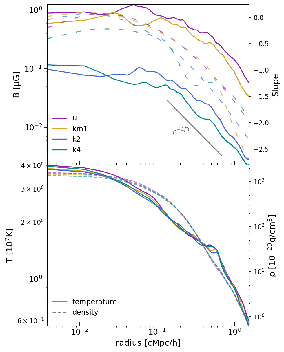
Figure 5: Radial profiles of the magnetic field (top) with the corresponding linear fits (dotted lines) for each magnetic seeding model, and density and temperature fields (bottom). All profiles are calculated in a sphere with $r=R_{\text{vir}}$ radius. In the outskirts, the magnetic field scales as $r^{-1.19},r^{-1.39},r^{-1.5},r^{-1.34}$ for the uniform, scale-invariant, Saffman, and Batchelor models, respectively.

The radial profiles of our cluster are shown in Figure 5. In the top panel, we show the magnetic field profiles, along with the expected trend from adiabatic flux freezing ($\propto r^{-4/3}$) and the slope profiles. As previously mentioned, we observe that those initial conditions with more magnetic power at large scales, such as the uniform and scale-invariant models, show the largest field strengths. Conversely, as shown in the bottom panel of Figure 5, neither in the trends of the slope nor in the radial temperature and density profiles do we observe any significant differences.

A commonly used proxy for relating the magnetic field and density distributions is combining their radial dependencies. In the outskirts ($r>150\,h^{-1}{\rm ckpc}$), this leads to $B_{\text{uni}}\propto\rho^{0.43}$, $B_{\text{inv}}\propto\rho^{0.50}$, $B_{\text{Saff}}\propto\rho^{0.54}$, and $B_{\text{Batch}}\propto\rho^{0.49}$ for the studied models. These trends are similar to those inferred from the radio observations of the massive $M_{200}\sim 1.8\times 10^{15}M_{\odot}$ (Kubo et al., 2007) Coma cluster (Bonafede et al., 2010), but are smoother than the slopes that have been found, e.g., in the observations of the less massive cluster $M_{200}\sim\times 10^{14}M_{\odot}$ (Girardi et al., 1998) A194 (Govoni et al., 2017). It should also be noted that the strength of the magnetic field in the core of the Coma cluster has been found to be higher ($4.7\,\mu{\rm G}$; Bonafede et al., 2010) than the obtained values from our simulations. This can be explained by the fact that the simulated galaxy cluster in our work is still dynamically young (see, e.g., Xu et al., 2011, who find that dynamically older relaxed clusters have larger magnetic field strengths in the ICM). In general, we find these trends to be in good agreement with the results of Vazza et al. (2018) and Domínguez-Fernández et al. (2019), where the authors having studied the dynamo amplification in the simulated galaxy clusters, also using AMR.

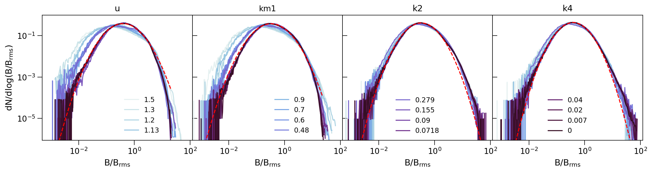
Figure 6: Redshift evolution of the PDFs. From left to right: the uniform, scale-invariant, helical, and nonhelical seedings. The PDFs are obtained within a sphere having $R_{\text{vir}}$ radius. The dashed red lines show the lognormal fits for each model.

4.3 Probability distribution function and curvature

The distribution of the magnetic fields has been the subject of several works. It follows from the induction equation that in the diffusion-free regime and at the kinematic stage of the dynamo (the weak-field limit), the magnetic field is characterized by a lognormal probability distribution function (PDF; see, e.g., Cho et al., 2002; Schekochihin et al., 2002, 2004; Brandenburg & Subramanian, 2005). The lognormality of the magnetic PDFs is qualitatively understood in terms of the central limit theorem, which is applied to the induction equation (without the diffusion term). A more rigorous derivation of this result involves the Kazantsev-Kraichnan dynamo model (Kazantsev, 1968; Kraichnan & Nagarajan, 1967). Following this model, it is possible to predict the evolution of the mean and the dispersion (see, e.g., Equations (5) and (6) in Schekochihin et al., 2002) of the lognormal distribution of the magnetic field. The spread of the PDF of $\log B$ at bobth the low and high tails of the distribution is an important characteristic of a lognormal distribution, meaning that a fluctuating magnetic field possesses a high degree of intermittency, i.e., the fluctuations tend to become more sparse in time and space and on smaller scales (see, e.g., Beresnyak & Lazarian 2019). In the saturated state of the dynamo, this intermittency is partially suppressed, and the PDF develops an exponential tail (see, e.g., Schekochihin et al. 2004 and the recent simulations of Seta & Federrath 2020).

In the following, we check whether dynamo action is present in our simulations. A comprehensive criterion for dynamo action in the presence of gravity is still missing; see Brandenburg & Ntormousi (2022) for some attempts. We follow the diagnostics presented in Schekochihin et al. (2004) which have also been used in Vazza et al. (2018) and Steinwandel et al. (2022).

In Figure 6, we show the evolution of the normalized magnetic field ($B/B_{\text{rms}}$) PDF for all four models. In the kinematic stage of the dynamo, Schekochihin et al. (2004) find that the magnetic PDF converges onto a single stationary profile, which is referred to as the self-similarity of the field strength. In our simulations, we find that the PDFs of the Saffman and Batchelor models resemble the stationary profile, while the large-scale models (uniform and scale-invariant) do not show the same behavior toward the low end tail of the PDF. The dispersions of the PDFs in the latter two cases decrease (although not significantly), while the dispersions of phase transition-generated models remain mostly constant. At the final redshift, we overplot a lognormal fit in Figure 6, and show that the low- and high-end tails of the distribution are reasonably well fitted by a lognormal distribution for all PMF models. Finally, we compute the kurtosis at $z=0$ and obtaine the values $12$, 13, 31, and $68$ for the uniform, scale-invariant, Saffman, and Batchelor models, respectively. These values confirm that all our models exhibit super-Gaussian profiles.

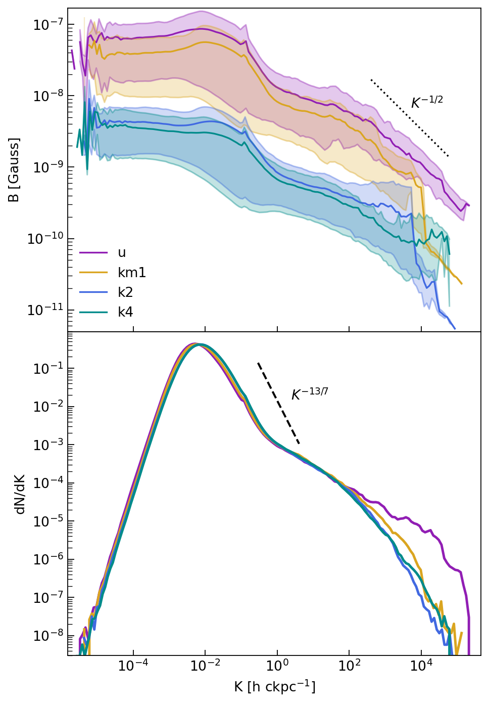
Figure 7: Profile of the magnetic field vs. curvature ($\mathbf{|K|}$) and the curvature PDFs calculated from a $(3.0\,h^{-1}{\rm cMpc})^{3}$ box at $z=0$. The dotted and dashed lines in the panels indicate the scalings that are expected from theoretical estimations (from Schekochihin et al., 2004). The shaded regions for each model cover the distribution points between the 16th and 84th percentiles.

The geometry of the magnetic field lines can be studied in terms of the curvature $\mathbf{K}$ defined as (e.g. Schekochihin et al., 2001):

$$\mathbf{K}=\frac{(\mathbf{B}\cdot\nabla)\mathbf{B}}{|\mathbf{B}^{2}|}=\frac{1}{\mathbf{B}^{2}}\bigg{[}\frac{1}{2}\nabla\mathbf{B}^{2}-\mathbf{B}\times(\nabla\times\mathbf{B})\bigg{]}.$$ (2)

In Figure 7, we show the dependence of the magnetic field on the absolute curvature, $K=|\mathbf{K}|$ (top panel) and the curvature distribution (bottom panel), at $z=0$. In small-scale dynamo theory, the turbulent amplification of the field proceeds by the stretching and bending of field lines by turbulent eddies, resulting in folded structures (see, e.g., Figures 1 and 2 of Schekochihin et al., 2002). Due to flux conservation arguments, it is expected that the magnetic field strength will be larger in the stretched segments of field lines, while the strength will remain small in the bends—i.e., the field strength and its curvature are expected to be anticorrelated. This is similar to an earlier finding that stronger flux tubes are also straighter (Brandenburg et al., 1995). The top panel of Figure 7 presents a good illustration of this hypothesis. We observe a declining profile of the magnetic field strength with increasing curvature of the field. This anticorrelation is confirmed by calculating the correlation coefficient between the curvature and the magnetic field $C_{K,B}$ (see Equation (26) in Schekochihin et al. 2004). For all our models at $z=0$, we obtain $C_{K,B}\sim-0.999$, which is practically its minimum possible value. We also note that this anticorrelation has already been observed from earlier redshifts in our simulations. At $z=0$, we obtain the slopes: $-0.32$ ($-0.46$), $-0.42$ ($-0.39$), $-0.35$ ($-0.47$), and $-0.25$ ($-0.34$) for the $(1.5\,h^{-1}{\rm cMpc})^{3}$ region ($(3\,h^{-1}{\rm cMpc})^{3}$ region), corresponding to the uniform, scale-invariant, Saffman, and Batchelor models, respectively. Another interesting feature that we see in the top panel of Figure 7 is the flattening of the magnetic field profile toward extremely low curvatures. From the bottom panel of Figure 7, we see that this happens for $K\lesssim 7\times 10^{-3}\,h\,{\rm ckpc^{-1}}$, where we observe a steep decrease ($\sim K^{2.5}$) in the curvature PDFs. The bulk of the curvature distribution is concentrated at the peak values corresponding to the $192$, 175, 140, and $143\,h^{-1}{\rm ckpc}$ scales (henceforth referred to as the curvature scales, $\lambda_{K}$) for the uniform, scale-invariant, Saffman, and Batchelor models, respectively. These scales reflect the typical bending scale of the field lines. As we shall see in Section 4.4.1, $\lambda_{K}$ is comparable to the scale containing the largest magnetic energy. We find that the peaks of the curvature PDFs shift to the right for all our models during the major merging phase, i.e., $\lambda_{K}$ decreases. This shows that mergers tend to further compress the existing folded structure, rather than elongating it. Finally, we also observe a distinctive difference between the uniform and stochastic models, with the former exhibiting the largest curvatures.

In summary, all of the PMF scenarios attain intermittent structures (the lognormality of the PDFs) during their evolutions even though the growth of the magnetic energy is relatively lower for the Saffman and Batchelor models (see Figure 4). (2) There is an anticorrelation between the field strength and the curvature for all models; however, the curvature scales are different for the large- and small-scale correlated fields. As a result, the different growth rates of the PMFs—i.e., the possible suppression or excitation of the dynamo—may leave imprints on the scale, where the further stretching and bending of the field lines is counteracted by the stronger fields.

4.4 Spectral evolution

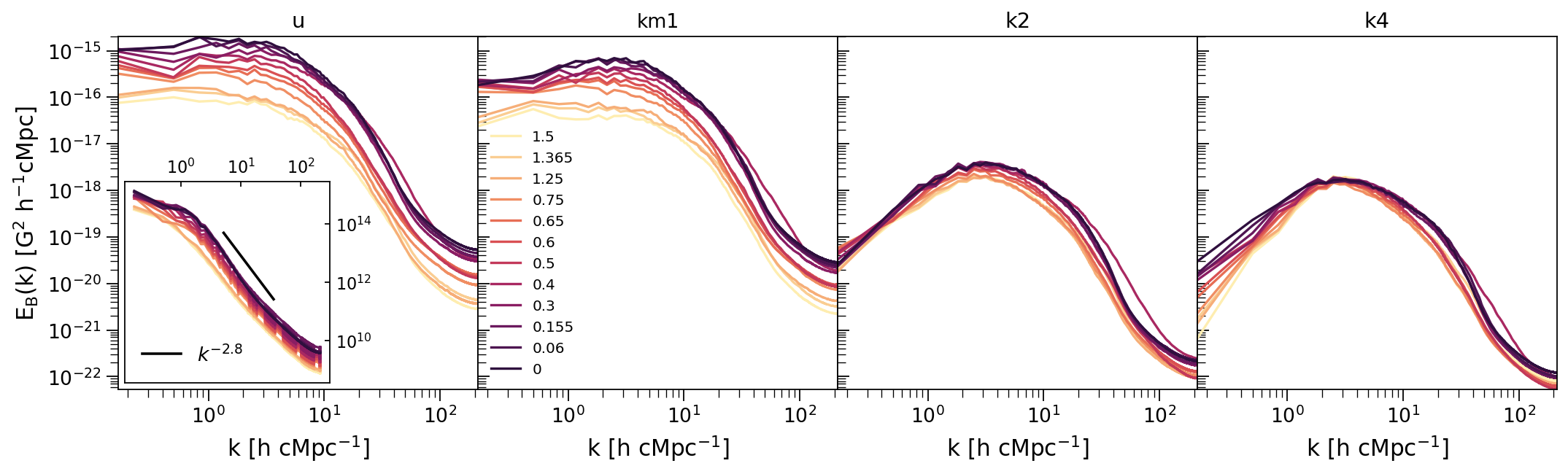
Figure 8: Redshift evolutions of the magnetic and the kinetic (inset in the left panel) energy spectra. From left to right: the uniform, scale-invariant, Saffman, and Batchelor models. The energy spectra are calculated from the $(3.0\,h^{-1}{\rm cMpc})^{3}$ box at the seventh level of AMR, using the yt interpolation method (Turk et al., 2011). For additional effects on the shapes and amplitudes of the magnetic energy spectra, we refer the reader to Appendix A. The axis units in the inset are $\,{\rm cm}^{2}\,{\rm s}^{-2}\,h^{-1}{\rm cMpc}$ and $\,h\,{\rm cMpc^{-1}}$, for the kinetic energy and wavenumbers, respectively.

In observations, previous knowledge of the magnetic energy spectrum is required, in order to obtain more information about the general characteristics of the magnetic fields in the ICM (see, e.g., Murgia et al., 2004; Govoni et al., 2006, 2017; Stuardi et al., 2021). The power spectrum of the magnetic field is defined as the Fourier transform of the magnetic field’s two-point correlation function, $\langle\mathbf{B}_{i}(\mathbf{x})\mathbf{B}_{j}(\mathbf{x}+\mathbf{r})\rangle$, where the angle brackets denote the ensemble average and $\hat{r}=r_{i}/|\mathbf{r}|$ (see Monin & I’Aglom 1971 or Brandenburg et al. 2018, and references therein). In practice, we define the magnetic energy power spectrum $E_{B}(k)$ through:

$$\int E_{B}(k)dk=\frac{1}{2V}\int\hat{\textbf{B}}\cdot\hat{\textbf{B}}^{*}4\pi k^{2}dk,$$ (3)

where $\hat{\textbf{B}}$ denotes the Fourier transform of the magnetic field, with $\hat{\textbf{B}}^{*}$ being its complex conjugate, $k=|\textbf{k}|$ is the norm of the wavevector, and $V$ is the volume that normalizes the spectrum.

In Figure 8 we show the evolutions of the magnetic energy spectra of our four models, with a specific kinetic energy spectrum for the uniform model being shown in the inset of the first panel. The magnetic spectrum is computed using Equation (3) for different time snapshots, in a $(3\,h^{-1}{\rm cMpc})^{3}$ simulation box, which follows the cluster center as it evolves. From the figure, one can see that differences between the spectra of the inflation- and phase transition-generated seed fields arise in both the amplitudes and the shapes of the magnetic power spectra. The differences observed in the shapes are more pronounced toward the largest scales ($\gtrsim 0.5\,h^{-1}{\rm cMpc}$) of the simulated galaxy cluster. In particular, at these scales, the spectra corresponding to the uniform and scale-invariant models are flatter than the spectra corresponding to the Saffman and Batchelor models. A similar result has also been found in Paper I. We will further discuss the shape of the magnetic energy spectrum in Section 4.4.2, where we parameterize our four cases. On the other hand, we note that the kinetic energy spectra (the inset in the left panel of Figure 8) of our simulations do not show differences between different PMF models. The spectra follow a $k^{\delta}$ profile, where $\delta$ changes between $\sim-2.3$ and $-2.8$ at small scales ($\lesssim 0.5\,h^{-1}{\rm cMpc}$) over the $9.5\,{\rm Gyr}$ time span.

In order to understand the differences in the magnetic field amplitudes between the different models, we recall that at early times ($10\lesssim z\lesssim 50$), before the cluster forms, only the uniform field model shows amplification homogeneously on all scales (see Figure 6 of Paper I), i.e., in the absence of gravitational accretion and induced turbulent motions, the stochastic models mostly stay frozen in or show an insignificant decay. At late times, as the cluster forms, the large-scale stochastic (i.e., the scale-invariant) model shows a similar trend as the uniform model and the amplitude of the power spectrum grows on all scales. This happens because the magnetic power is concentrated on the largest scales, similar to the power corresponding to the density and velocity fields (this can be seen in Figure 1 in which we show our selected initial density and velocity power spectra, as well as in the inset in the first panel of Figure 8). In addition, when turbulence develops, it first produces large-scale eddies that stretch and bend the field lines of those models where the large-scale magnetic component is present. In the stochastic small-scale models, magnetic amplification happens after turbulence cascades down to scales comparable to the corresponding magnetic coherence scales. Therefore, the magnetic energy of these models (Saffman and Batchelor) is prone to less efficient and slower growth. Furthermore, as Schekochihin et al. (2001) have pointed out, a chaotically tangled field will decay toward a folding state at a rate comparable to the rate of the magnetic energy growth. Thus, the initial slower growth in the Saffman and Batchelor models will further suppress the folding of the field lines, leading overall to a lesser amplification degree in these models.

We note that the different growth rates (see also Figure 4) for large- and smaller-scale magnetic fields obtained in our simulations are at odds with the results of driven-turbulence simulations; see e.g., Cho et al. (2009) and Seta & Federrath (2020) who compare the evolutions of uniform (imposed) and random (stochastic) fields in incompressible and compressible MHD turbulence settings, respectively. Nonetheless, these authors also find a delay in the onset of the linear growth for low initial field strengths (the uniform field case; Cho et al., 2009) or a decay during the initial transient phase (the random field case; Seta & Federrath, 2020). In the latter work, the uniform model does not decay, and it shows rapid growth during this phase; this trend is similar to the results presented in our work. Contrary to the results of driven-turbulence MHD simulations (see, e.g., Schekochihin et al., 2004; Brandenburg et al., 2015), our study does not clearly indicate forward or inverse cascading either. However, we must bear in mind that the ICM is a complex system, in which mergers might alter the aforementioned trends that we have discussed above.

4.4.1 Characteristic scales

A clearly visible characteristic of the magnetic energy spectrum is the peak scale $L_{E_{B}(k)}$ corresponding to $1200$ and $400\,h^{-1}{\rm ckpc}$ for the uniform and scale-invariant models, respectively, and to $316\,h^{-1}{\rm ckpc}$ scales for the Saffman and Batchelor models. To determine the largest energy-containing scale of the magnetic field (see the definition in Cho & Ryu, 2009), we also calculated the peak scale of $kE_{B}(k)$, i.e, the peak scale of the spectral energy per mode. We find similar values of $L_{kE_{B}(k)}$ for all our models: $222\,h^{-1}{\rm ckpc}$ for the uniform and scale-invariant models and $171$ and $154\,h^{-1}{\rm ckpc}$ for the Saffman and Batchelor models. We also find that the peak scales of the density, $L_{kP_{\rho}(k)}$, and velocity, $L_{kE_{v}(k)}$ spectral energy per mode are the same: $\sim 857\,h^{-1}{\rm ckpc}$. In the inflationary and phase-transitional models, $L_{kE_{B}(k)}$ is $\sim$ one-fourth and $\sim$ one-fifth of $L_{kE_{\rho}(k)}$ and $L_{kE_{v}(k)}$, respectively. A similar result has also been found in the MHD simulations of Cho & Ryu (2009) where the authors find a $\sim 1/5$ ratio at the saturation between $L_{kE_{B}(k)}$ and the driving (injection) scale of turbulence. Therefore, our results suggest that most of the magnetic energy resides on scales that are smaller than the gravity-induced scale or the peak scale of the density and velocity power spectra.

The correlation length, which is also referred to as the coherence or integral scale, of the magnetic field is defined as:

$$\lambda=\frac{\int_{0}^{\infty}dk\,k^{-1}E_{B}(k,t)}{\int_{0}^{\infty}dk\,E_{B}(k,t)}.$$ (4)

The evolutions of the magnetic correlation lengths for the different PMF models are shown in the top panel of Figure 9. We computed the correlation length throughout the $12$ Gyr period, focusing on a $(1.5\,\,h^{-1}{\rm cMpc})^{3}$ region (as in Figure 4). We also conducted the same analysis in a $(3.0\,\,h^{-1}{\rm cMpc})^{3}$ region, since the correlation length can depend on the box size under consideration. During merger events (shown as the vertical shaded areas in Figure 9), the magnetic correlation length decreases for all four models. This happens mainly because compression becomes dominant as the infalling gas clump crosses the cluster center. The same effect has also been observed in other cosmological MHD simulations, e.g. in Domínguez-Fernández et al. (2019), where the authors find that major merger events shift the magnetic power toward smaller scales. It is after each merger event that the magnetic correlation length increases again for all four models.

Figure 9: Evolutions of magnetic correlation lengths (top panel) and characteristic parallel and perpendicular scales (bottom panel) for the simulated galaxy cluster. The vertical shaded regions show merging phases during the evolution of the galaxy cluster. The horizontal shaded areas in the top panel are delimited according to the analyzed region; the lower (upper) lines correspond to a $(1.5\,h^{-1}{\rm cMpc})^{3}$ ($(3.0\,h^{-1}{\rm cMpc})^{3}$) region.

Finally, as the cluster enters its relaxing phase at $z\lesssim 0.135$, the correlation lengths for all models converge to $260$–$410$, $240$–$330$, $180$–$230$, and $170$–$240\,h^{-1}{\rm ckpc}$ for the uniform, scale-invariant, Saffman, and Batchelor models, respectively. These values are one order of magnitude larger than those that are obtained and typically referred to as the coherence scale (a few tens of kiloparsecs) from radio observations (see, e.g., Murgia et al., 2004; Vogt & Enßlin, 2005; van Weeren et al., 2019). The strongest differences in the magnetic correlation lengths between the models are better seen at earlier redshifts, where the scale-invariant model shows a coherence length that is larger than those of the Saffman and Batchelor models by a factor of $\sim 2$. We note that while the differences between the uniform and scale-invariant models and those between the Batchelor and Saffman models decrease after the merger events, we still observe larger correlation lengths in the inflationary cases than in the phase-transitional scenarios throughout the evolution of the galaxy cluster over this 12 Gyr period.

Following Schekochihin et al. 2004, one can also define the characteristic wavenumbers,

$$\begin{gathered}k_{\parallel}=\bigg{(}\frac{\langle|\mathbf{B\cdot\nabla\mathbf{B}}|^{2}\rangle}{\langle B^{4}\rangle}\bigg{)}^{1/2},~{}~{}k_{\mathbf{B}\times\mathbf{J}}=\bigg{(}\frac{\langle|\mathbf{B\times\mathbf{J}}|^{2}\rangle}{\langle B^{4}\rangle}\bigg{)}^{1/2}\end{gathered}$$ (5)

corresponding to the magnetic field variation along ($k_{\parallel}$) and across ($k_{\mathbf{B}\times\mathbf{J}}$) itself, with $\mathbf{J}$ being the current density. In small-scale dynamo theory, it has been argued that generally $k_{\mathbf{B}\times\mathbf{J}}>k_{\parallel}$ since the shear flows can more rapidly stretch and reverse the field lines in the plane transverse of the field line itself (see Schekochihin et al., 2001, and references therein). In other words, the growth of the typical fluctuation wavenumber $k=\sqrt{k_{\mathbf{B}\times\mathbf{J}}^{2}+k_{\parallel}^{2}}$ should mostly be due to the increase of $k_{\mathbf{B}\times\mathbf{J}}$. It has been shown that in both the MHD dynamo (Schekochihin et al., 2004) and the plasma dynamo (St-Onge & Kunz, 2018), the $k_{\mathbf{B}\times\mathbf{J}}>k_{\parallel}$ ordering is satisfied in the initial, rapid growth phase and that is persists in the kinematic and nonlinear regime of a dynamo (during saturation).

In the bottom panel of Figure 9 we show the evolution of the $\lambda_{\parallel},\lambda_{\mathbf{B}\times\mathbf{J}}$, scales corresponding to the inverse $k_{\parallel}$, $k_{\mathbf{B}\times\mathbf{J}}$, characteristic wavenumbers, respectively. The condition $k_{\mathbf{B}\times\mathbf{J}}>k_{\parallel}$ is satisfied for $z<3$ in the simulated cluster for all four magnetic cases. We find a maximum ratio of $k_{\mathbf{B}\times\mathbf{J}}/k_{\parallel}\sim 2-3$ over the 12 Gyr period. The ordering of these characteristic scales seems to be consistent with the arrangement of a magnetic field in folded structures; see also Figure 23(a) of Schekochihin et al. (2004). This result, along with the lognormarlity of the PDFs and curvature results, would be compatible with the kinematic stage of a dynamo in our simulations.

4.4.2 Parameterization of magnetic energy spectra

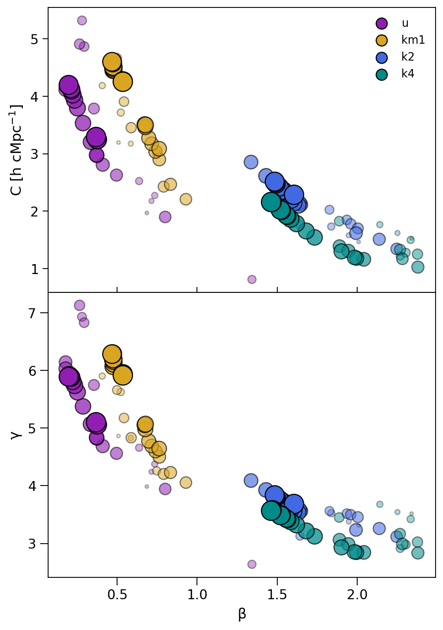
Figure 10: Parameter spaces for the best-fit parameters of our different PMF models considering a $(3.0\,h^{-1}{\rm cMpc})^{3}$ region. The smaller markers and the lower-opacity colors show the parameters at early times. The top and bottom panels show the results from the fits according to Equations (6) and (7), respectively.

In order to discriminate among the magnetic field models we characterize the magnetic energy spectra in the $(3\,\,h^{-1}{\rm cMpc})^{3}$ box. We consider two different fitting functions. First, we use the equation

$$E_{B}(k)=Ak^{\beta}\left\{1-\text{erf}\left[B\,\ln\left(\frac{k}{C}\right)\right]\right\},$$ (6)

where $A$ gives the normalization, $B$ is related to the width of the spectra, $C$ is a characteristic wavenumber of the magnetic field, and $\beta$ is the slope of the spectrum at small wavenumbers. This fitting function has been used in Domínguez-Fernández et al. (2019) to study the evolutions of the magnetic energy spectra for a set of highly resolved galaxy clusters, assuming a uniform magnetic field seeding. The large-scale slope used by the authors satisfies the Kazantsev (Kazantsev, 1968; Kulsrud & Anderson, 1992) scaling, $\beta=3/2$. We use a similar approach, by fitting Equation (6) to the magnetic energy spectra of our simulated cluster and obtaining the best-fit parameters $A$, $B$, and $C$. In our case, we fix the initial $\beta$ at each time step separately. That is, as a first step, we determine the large-scale slope of the spectra, $\beta$, and, as a second step, we fix this value in the fitting equation.

The second fitting function is motivated by the MHD simulations in Brandenburg et al. (2017), where a phase transition-generated magnetic field has a pronounced peak on the scale of the field generation. We adopt the following spectral shape (Brandenburg et al., 2017; Roper Pol et al., 2022):

$$E_{B}(k)=(1+D)^{1/\alpha}E_{\rm m}\frac{(k/k_{*})^{\beta}}{[1+D(k/k_{*})^{\alpha(\beta+\gamma)}]^{1/\alpha}},$$ (7)

where $D$ controls the peak scale, $E_{\rm m}$ is the normalization, $k_{*}$ is the peak wavenumber, and $\beta$ and $\gamma$ are the slopes at large ($k<k_{*}$) and small ($k>k_{*}$) scales, respectively. The value of $\alpha$ is chosen to be $0.25$, to ensure a smooth transition between the spectra on large and small scales. In this case, $D,E_{\rm m},$ and $\gamma$ are the best-fit parameters obtained. Figure 10 summarizes the results of our fitting procedure, using Equations (6) and (7). We only show only the most important best-fit parameters for each model in Figure 10, while we provide all the parameters at $z=0$ in Table 3. In the upper panel, we show the $C-\beta$ parameter space (see Equation (6)), and in the lower panel we show the $\gamma-\beta$ parameter space (see Equation (7)). We show the evolutions of the fitting parameters over a time span of $6.1\,{\rm Gyr}$ in the redshift range of $0.63\leq z\leq 0$. As it can be seen from Figure 9, this period encompasses a major merger event at $z\sim 0.48$ and the relaxing phase of the cluster.

Table 3: Parameters of the power spectra for different models and for different fitting functions at $z=0$. The power spectra are fitted with Equations (6) and (7). The fixed $\beta$ parameters are: $0.37$, 0.54, 1.61, $1.46$ for the uniform, scale-invariant, Saffman, and Batchelor models, respectively, with $\alpha=0.25$.

Model	Eq.	A    $[\mathrm{G}^{2}\,h^{-1}{\rm cMpc}]$	B	C $[\,h\,{\rm cMpc^{-1}}]$
		$E_{\rm m}$    $[\mathrm{G}^{2}\,h^{-1}{\rm cMpc}]$	D	$\gamma$
u	(6)	$8.92\times 10^{-16}$	2.16	3.29
	(7)	$1.63\times 10^{-15}$	0.03	5.10
km1	(6)	$2.54\times 10^{-16}$	2.56	4.25
	(7)	$6.44\times 10^{-16}$	0.095	5.92
k2	(6)	$8.66\times 10^{-19}$	2.27	2.29
	(7)	$3.57\times 10^{-18}$	0.403	3.68
k4	(6)	$4.91\times 10^{-19}$	2.17	2.16
	(7)	$1.62\times 10^{-18}$	0.427	3.57

The $C$–$\beta$ and $\gamma$–$\beta$ parameter spaces highlight how the spectral characteristics of the inflationary cases differ from those of the phase-transitional cases. In the following, we discuss the main points.

• The evolution of the $C$ parameter varies between $2$–$4.5\,\,h\,{\rm cMpc^{-1}}$ for the inflationary models and between $1$–$2.8\,h\,{\rm cMpc^{-1}}$ for the phase transitional models. The ratio between the magnetic correlation length and $1/C$ is $\sim 1.4$ for the inflationary models and $\sim 0.5$ for the phase-transitional seedings. That is, $\lambda_{B}\gtrsim 1/C$ for the former scenarios and $\lambda_{B}\lesssim 1/C$ for the latter models. This shows that this fitting equation is a good proxy for obtaining a characteristic scale of the magnetic field that can be comparable to or of the same order as $\lambda_{B}$.

• The large-scale slopes of the magnetic power spectra characterized by $\beta$ deviate from a Kazantsev slope in the inflationary models where $\beta\lesssim 1$. In contrast, the phase-transitional models are approximately characterized by a Kazantsev slope at late redshifts. These models show a scatter in the range $1.2\lesssim\beta\lesssim 2.5$, where the slope tends to flatten progressively toward $\sim 3/2$ as the cluster virializes.

• The small-scale slopes of the magnetic power spectra characterized by $\gamma$ vary between $3.9$ and $6.5$ in the inflationary models and $2$ and $4.1$ in the phase-transitional models. As seen from Figure 8, the magnetic energy growth at scales larger than the characteristic scale is more pronounced in the two inflationary cases, therefore explaining the larger values of $\gamma$ compared to those from the phase-transitional models.

Finally, we note that we refrain from claiming that the phase-transitional models can corroborate the 3/2 large-scale slope predicted by the Kazantsev model since, as can be seen from Figures 8 and 10, this slope can vary throughout the complex evolution of galaxy clusters. Indeed, the multiple merger events that lead to the final formation of a cluster already break down one of the most basic assumptions of Kazantsev theory—i.e., a delta-correlated (in time) velocity field.

5 Numerical aspects

The numerical resolution is an important caveat to the analysis conducted in this work. Similar simulations presented by Vazza et al. (2014, 2018) have shown that magnetic fields tend to be more strongly affected by resolution effects than the velocity field, for example. Therefore, the growth rates of the seed magnetic fields in galaxy clusters are also resolution-dependent. Within our numerical setup, we assess the convergence of our results by performing extra simulations with different AMR levels. In Appendices A and B, we show how the power spectra, the PDFs, and the radial profiles of the magnetic field have already converged at six AMR levels (on scales $\gtrsim 50\,h^{-1}{\rm ckpc}$).

As in Paper I, we rely on the Dedner cleaning algorithm (Dedner et al., 2002) to impose the $\nabla\cdot\mathbf{B}=0$ condition. While the Dedner formalism has been found to be robust and accurate, as well as to converge quickly on the right solution for most idealized test problems (Wang & Abel, 2009; Wang et al., 2010; Bryan et al., 2014), and for other more realistic astrophysical applications (Hopkins & Raives, 2016; Tricco et al., 2016; Barnes et al., 2018), this method may be limited compared to the constrained transport (CT) schemes (Kritsuk et al., 2011). The intrinsic dissipation of the Dedner scheme, via cleaning waves, can affect the final magnetic growth of our PMF models. Divergence cleaning has also been associated with spurious magnetic helicity production (Brandenburg & Scannapieco, 2020). Consequently, we cannot entirely rule out the possibility numerics (see also Appendix C of Paper I) can also contribute to the obtained differences between the growth rates of the inflationary and phase-transitional models. In Figure 12 of Appendix A, we show the radial profile of the magnetic field divergences in our simulated cluster. The densest central region of the cluster exhibits a similar normalized divergences for our four PMF models, while some differences between the inflationary and phase-transitional cases can only be observed at large radii, $\gtrsim 1.2\,h^{-1}{\rm cMpc}$, with the former case showing the lowest values. Nevertheless, the Dedner cleaning method keeps the numerical magnetic field divergence below $\sim 5$% ($\sim 8$%) of the local magnetic field within the cluster volume having $r=R_{500}$ ($r=R_{100}$) radius. This shows that the divergence remains reasonably low in the largest fraction of the simulated cluster volume. We leave a numerical comparison between the Dedner and CT schemes within the Enzo code in the context of PMFs in galaxy clusters for future work.

As mentioned in Section 3, we have only focused on the amplification of PMFs, due to the structure formation and turbulent motions in the ICM. However, the inclusion of additional physics, such as feedback and radiative cooling physics, could lead to larger amplification levels of our PMF models, and may therefore affect the final magnetic fields (see e.g., Marinacci et al., 2015; Vazza et al., 2017). The effects of these processes on distinguishing between different magnetogenesis scenarios will also be studied in our future work.

6 Conclusions

In this work, we have investigated the evolution of PMFs during the formation of a massive galaxy cluster. We have studied seed magnetic fields resembling inflation- and phase transition-generated nonhelical fields. In the former case, we have assumed either (1) a uniform, constant magnetic field or (2) a stochastic field. The stochastic model is motivated by the pre-recombination evolution of an inflationary seed field (initially having a scale-invariant spectrum), while the uniform case corresponds to the Mukohyama model. In the case of phase transition-generated seed magnetic fields, we have studied stochastic models with initial (3) Batchelor and (4) Saffman spectra. These magnetic spectra are motivated by the causal generation and evolution of phase-transitional fields until recombination.

The main results of our work can be summarized as follows.

• Final amplification. The amplification of a primordial seed magnetic field in the ICM strongly depends on the initial structure of the magnetic field. In our simulated galaxy cluster, the inflation-generated uniform and scale-invariant models show more efficient amplification compared to the phase transition-generated Saffman and Batchelor models. We see that in the former cases the magnetic energy density is of the same order of magnitude as the turbulent energy budget of the cluster. In such cases, the magnetic power is concentrated on the largest scales, similar to the power corresponding to the density and velocity fields. This leads to more efficient turbulent amplification of these large-scale models compared to the small-scale phase-transitional seed magnetic fields.

• Radial profiles. The radial magnetic field profiles at the final redshift ($z=0$) reflect the aforementioned differences in the magnetic energy growth. The amplitude of the uniform and scale-invariant models is one order of magnitude larger ($\sim 0.8$–$1\,\mu{\rm G}$; cluster center) than the amplitude attained by the phase transition-generated magnetic fields ($\sim 0.1\,\mu{\rm G}$). The declining magnetic field profile toward the outskirts reveals the largest differences between the uniform ($r^{-1.19}$) and the Saffman ($r^{-1.5}$) models.

• Small-scale dynamo. All of our models exhibit a degree of small-scale dynamo amplification, as hinted at by the lognormality of the magnetic field PDFs and the folded structures of field lines (i.e., the anticorrelation between the field strength and curvature and the ordering of the characteristic wavenumbers). Consistent with the previous works (Vazza et al., 2018; Domínguez-Fernández et al., 2019; Steinwandel et al., 2022), we find that cosmological MHD simulations do not exhibit a small-scale dynamo that can be compared one-to-one to the Kazantsev theory.

• Coherence lengths. We find that, throughout the evolution, the magnetic correlation length of the cluster depends on both the initial structure of the seed field and the merger history. We find that the inflationary models (initially large-scale correlated PMFs) will inherently attain larger coherence lengths than the phase-transitional models, throughout the evolutions of galaxy clusters. This trend is even persistent during merger events, where the correlation length decreases for all models. At the final redshifts, we observe a factor of $\sim 1.5$ difference in the coherence scales of the uniform and scale-invariant models versus the Batchelor and Saffman models. The correlation lengths calculated from a $[(1.5$–$3)\,h^{-1}{\rm cMpc}]^{3}$ analyzing box span in the range: $260$–$410$, $240$–$330$, $180$–$230$, and $170$–$240\,h^{-1}{\rm ckpc}$ for the uniform, scale-invariant, Saffman, and Batchelor models, respectively.

• Spectral characteristics. We provide two possible fits for the magnetic energy spectra. The parameterization of the magnetic energy spectra shows how phase-transitional and inflationary models can be differentiated. The large-scale slopes (the $\beta$ parameter; see Section 4.4.2) are smaller ($\lesssim 1$) for the inflationary PMFs, but larger ($1.2\lesssim\beta\lesssim 2.5$) for the phase-transitional PMFs, over a time span of $6.1$ Gyr ($0.63\leq z\leq 0$). The Batchelor and Saffman models have Kazantsev scaling ($\beta=3/2$) at the final redshifts, even though these fields are amplified to a lesser degree. On the contrary, the small-scale slopes (the $\gamma$ parameter; see Section 4.4.2) are larger for the inflationary models ($\gamma\sim 3.9$–$6.5$) than for the phase-transitional seedings ($\gamma\sim 3.9$–$6.5$). The $1/C$ scales at the final redshift are $300\,h^{-1}{\rm ckpc}$, $240\,h^{-1}{\rm ckpc}$, $440\,h^{-1}{\rm ckpc}$, and $460\,h^{-1}{\rm ckpc}$ for the uniform, scale-invariant, Saffman, and Batchelor models, respectively.

In summary, we conclude that the two competing scenarios of primordial magnetogenesis, inflationary and phase-transitional, can indeed be distinguished on galaxy cluster scales. The initial structure of the seed magnetic field affects the efficiency of the dynamo. Thus, PMFs do not only leave unique imprints on scales larger than those of galaxy clusters (Paper I), but it can also influence small-scale dynamo action in the ICM. These signatures are reflected in the magnetic energy power spectrum and the coherence scale of different models. An analytical power spectrum of the magnetic field is required for synthetic RM studies (see the method description in, e.g., Stuardi et al., 2021), giving us the possibility to constrain the structure of observed galaxy cluster magnetic fields. We provide two analytical models that can readily be used in observational works (see, e.g., Murgia et al., 2004; Bonafede et al., 2013; Govoni et al., 2017, for such examples).

Finally, since the inflationary models show larger field strengths (both in the centers as well as on the outskirts of the simulated clusters) and coherence scales, these may make them better candidates for producing e.g., the central cluster radio diffuse emission in the form of the “megahalos” that have been recently detected with LOFAR (Cuciti et al., 2022). Megahalos fill a volume 30 times larger than do common radio halos. This makes them interesting objects for unveiling the nature of relativistic electrons and magnetic fields on the outskirts of galaxy clusters. On the other hand, inflationary magnetogenesis scenarios would be also favored for obtaining the fast magnetic field amplification that is needed to explain the observed diffuse radio emission in high-redshift galaxy clusters (Di Gennaro et al., 2021). Deeper observations of megahalos, together with the detailed RM images that will be obtained by future observations with the Square Kilometre Array (SKA) and the upgraded LOFAR 2.0, will have the potential to unravel the origins of large-scale magnetic fields.

Data Availability

The derived data supporting the findings of this study are available from the corresponding author upon request.

Software: The source codes used for the simulations of this study—Enzo (Brummel-Smith et al., 2019) and the Pencil Code (Pencil Code Collaboration et al., 2021)—are freely available online, at https://github.com/enzo-project/enzo-dev and https://github.com/pencil-code/.

Appendix A Resolution tests and Divergence

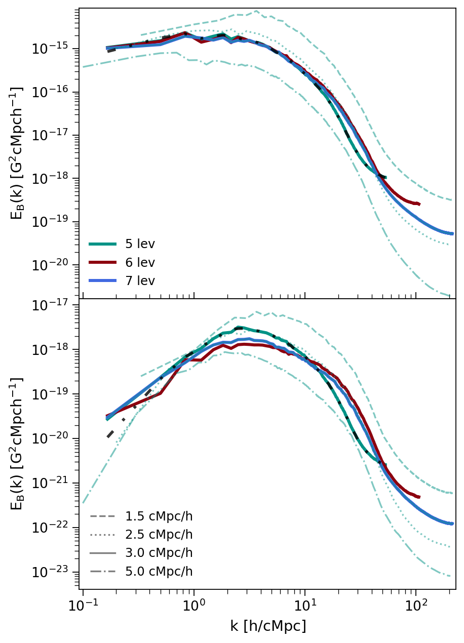
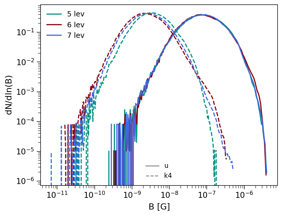
Figure 11: Upper panels: magnetic energy power spectra calculated for different AMR levels and different box sizes at $z=0$. We show the uniform (top panel) and Batchelor (middle panel) cases. The black dashed-dotted lines in each panel show the power spectra calculated from a zero-padded array. Lower panel: magnetic field PDFs of the uniform (solid lines) and Batchelor (dashed lines) models at $z=0$, at different AMR levels.

In this appendix, we discuss the dependence of our results on the adopted spatial resolution. We use the same initial conditions and perform different simulations, increasing the levels of AMR. We show the results corresponding to a maximum of $5$, $6$ and $7$ levels of AMR in Figure 11. The dependence on spatial resolution of the magnetic power spectra and the PDFs of the magnetic field are shown by the different colors. Even though we see greater variation for the Batchelor model (the middle panel and the dashed lines of the bottom panel), we already observe the convergence of both the uniform and Batchelor models already at the sixth level of AMR and we see no significant changes in the shapes of the magnetic energy spectra.

Spectral analysis based on Fourier transforms is a common approach studying the scale dependence of the magnetic energy. Nevertheless, some caveats to this approach result from the effects of a limited box size and the nonperiodicity of the data. In Figure 11, we show the outcomes of these effects on the magnetic energy spectra for the simulated uniform and Batchelor models. First, we see that for $k\lesssim 50\,h\,{\rm cMpc^{-1}}$, corresponding to scales $\gtrsim 20\,h^{-1}{\rm ckpc}$, the spectra are well converged in the uniform model. The shape of the magnetic spectra for both the uniform and Batchelor models are also mostly consistent with the spectra calculated in smaller/larger boxes. As expected, the amplitudes of the spectra are more strongly affected by the size of the analyzed regions. In particular, we see a $\sim$ one order of magnitude variation on the scales of $\sim 140\,h^{-1}{\rm ckpc}$ for the uniform as well as Batchelor models.

We also note that the nonperiodic boundary conditions of the selected box may distort the spectrum. In order to check this, we calculate the power spectra from the zero-padded array, extracted for the $(3\,h^{-1}{\rm cMpc})^{3}$ volume from the five-level-AMR simulation (see the black dashed-dotted lines in Figure 11). As seen in the figure, the power spectra calculated using the standard method and zero padding lead to similar results, revealing that our results as presented in the main text are not significantly affected by the nonperiodicity of the data.

Finally, in Figure 12 we show the radial profiles of the magnetic field divergence in our simulated cluster. The largest differences between the models arise at $r\gtrsim 1\,h^{-1}{\rm cMpc}$, with the stochastic models having the largest values of divergence. Nevertheless, as mentioned in Section 5, $\nabla\cdot\mathbf{B}$ stays reasonably low in our four models in the largest fraction of the simulated cluster volume. Quantitatively, we find that the normalized divergence remains below 10%.

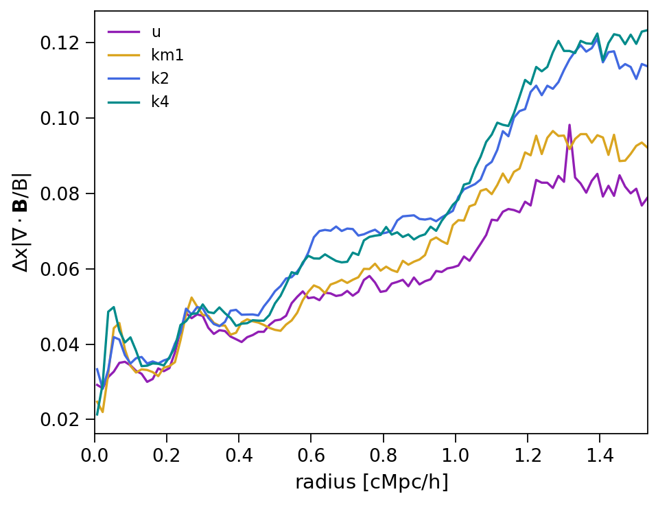
Figure 12: Normalized divergences of the magnetic fields from the simulation with a maximum of seven levels of AMR (where $\Delta$ is the mesh spacing in the $x$-direction).

Appendix B Distribution of AMR levels

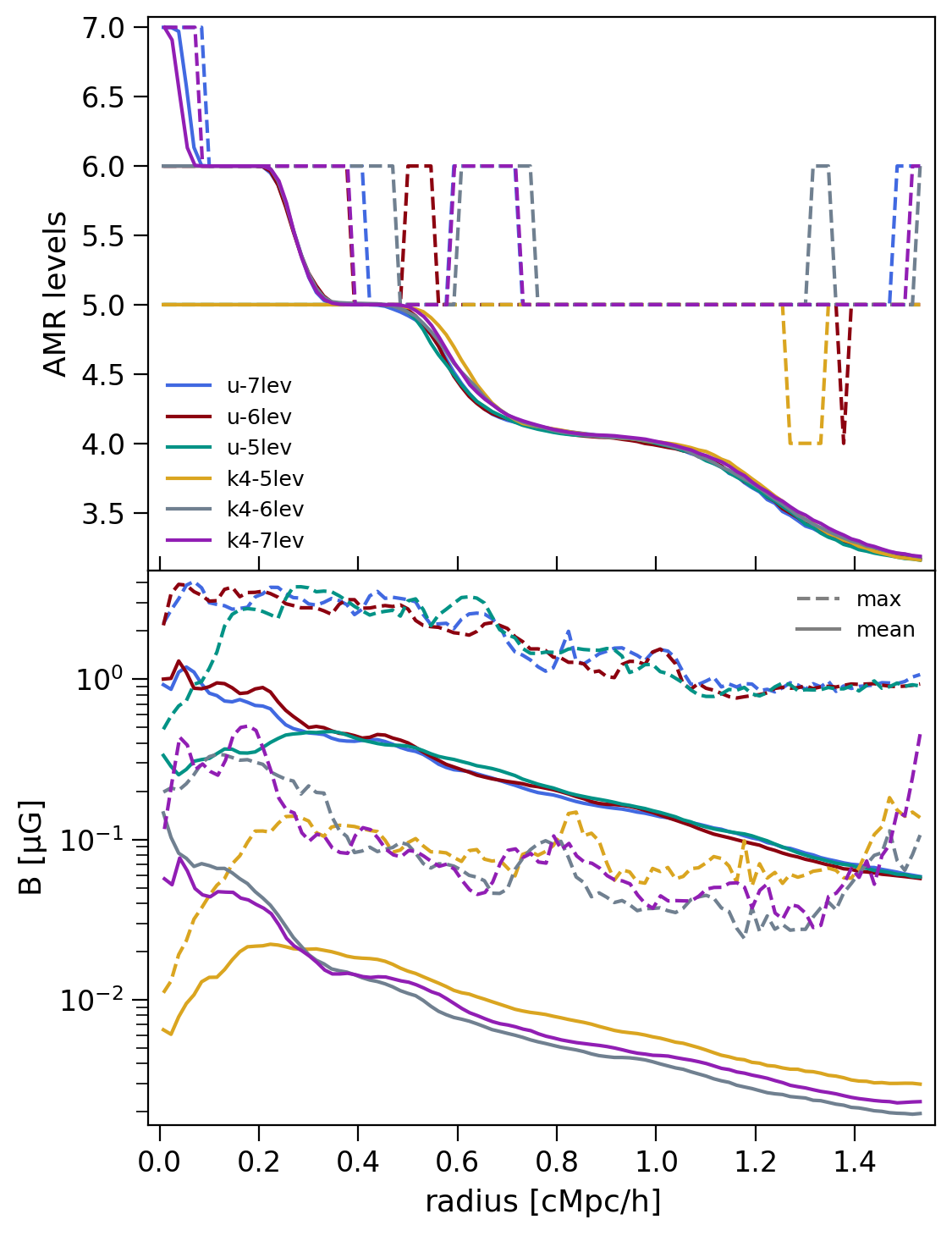
Figure 13: Radial distributions of the refinement levels and magnetic fields. The mean and maximum within each radial bin are shown by the solid and dashed lines, respectively. The profiles are shown for the uniform and Batchelor models, calculated from a sphere with an $R_{\text{rvir}}$ radius.

Similar to Vazza et al. (2018), we show the radial profiles of the AMR levels along with the magnetic field profile in Figure 13, for the uniform and Batchelor cases. In the top panel of Figure 13 we see that our simulated cluster is resolved with a maximum of five AMR levels (with $9.77\,h^{-1}{\rm ckpc}$ resolution) in the $(1.5\,\,h^{-1}{\rm cMpc})^{3}$ central region, while the mean AMR level decreases toward the outskirts. On the other hand, the magnetic field profiles (the bottom panel of Figure 13) show larger strengths only in the cluster core when the maximum levels of AMR are increased from five to seven. Our AMR scheme is different from the one used in Vazza et al. (2018) where the cluster is refined up to at least a sixth AMR level, even on the cluster outskirts. An important difference, however, between the simulated clusters used in this work and those used in Vazza et al. (2018) is the mass of the cluster, which is one order of magnitude larger in the latter work.

In addition, we check the convergence of our AMR scheme by running an extra simulation with a maximum of eight levels of AMR (for the Batchelor model, not shown). We do not see an important improvement in the AMR coverage of the cluster region when using higher levels of AMR. Therefore, given our selected refinement parameters, our AMR scheme already converges at six AMR levels.

References

- Ackermann et al. (2018) Ackermann, M., Ajello, M., Baldini, L., et al. 2018, ApJS, 237, 32, doi: 10.3847/1538-4365/aacdf7
- Ahonen & Enqvist (1998) Ahonen, J., & Enqvist, K. 1998, Phys. Rev. D, 57, 664, doi: 10.1103/PhysRevD.57.664
- Banerjee & Jedamzik (2004) Banerjee, R., & Jedamzik, K. 2004, Phys. Rev. D, 70, 123003, doi: 10.1103/PhysRevD.70.123003
- Barnes et al. (2018) Barnes, D. J., On, A. Y. L., Wu, K., & Kawata, D. 2018, MNRAS, 476, 2890, doi: 10.1093/mnras/sty400
- Beresnyak & Lazarian (2019) Beresnyak, A., & Lazarian, A. 2019, Turbulence in Magnetohydrodynamics (Berlin, Boston: De Gruyter), doi: doi:10.1515/9783110263282
- Bertone et al. (2006) Bertone, S., Vogt, C., & Enßlin, T. 2006, MNRAS, 370, 319, doi: 10.1111/j.1365-2966.2006.10474.x
- Biermann (1950) Biermann, L. 1950, Zeitschr. Naturforsch. A, 5, 65
- Bonafede et al. (2010) Bonafede, A., Feretti, L., Murgia, M., et al. 2010, A&A, 513, A30, doi: 10.1051/0004-6361/200913696
- Bonafede et al. (2013) Bonafede, A., Vazza, F., Brüggen, M., et al. 2013, MNRAS, 433, 3208, doi: 10.1093/mnras/stt960
- Bondarenko et al. (2022) Bondarenko, K., Boyarsky, A., Korochkin, A., et al. 2022, A&A, 660, A80, doi: 10.1051/0004-6361/202141595
- Botteon et al. (2021) Botteon, A., Cassano, R., van Weeren, R. J., et al. 2021, ApJ, 914, L29, doi: 10.3847/2041-8213/ac0636
- Brandenburg et al. (2020) Brandenburg, A., Durrer, R., Huang, Y., et al. 2020, Phys. Rev. D, 102, 023536, doi: 10.1103/PhysRevD.102.023536
- Brandenburg et al. (2018) Brandenburg, A., Durrer, R., Kahniashvili, T., Mandal, S., & Yin, W. W. 2018, J. Cosmology Astropart. Phys, 2018, 034, doi: 10.1088/1475-7516/2018/08/034
- Brandenburg et al. (1996) Brandenburg, A., Enqvist, K., & Olesen, P. 1996, Phys. Rev. D, 54, 1291, doi: 10.1103/PhysRevD.54.1291
- Brandenburg et al. (2017) Brandenburg, A., Kahniashvili, T., Mandal, S., et al. 2017, Phys. Rev. D, 96, 123528, doi: 10.1103/PhysRevD.96.123528
- Brandenburg et al. (2015) Brandenburg, A., Kahniashvili, T., & Tevzadze, A. G. 2015, Phys. Rev. Lett., 114, 075001, doi: 10.1103/PhysRevLett.114.075001
- Brandenburg & Ntormousi (2022) Brandenburg, A., & Ntormousi, E. 2022, MNRAS, 513, 2136, doi: 10.1093/mnras/stac982
- Brandenburg et al. (1995) Brandenburg, A., Procaccia, I., & Segel, D. 1995, Phys. Plasmas, 2, 1148, doi: 10.1063/1.871393
- Brandenburg et al. (2023a) Brandenburg, A., Rogachevskii, I., & Schober, J. 2023a, MNRAS, 518, 6367, doi: 10.1093/mnras/stac3555
- Brandenburg & Scannapieco (2020) Brandenburg, A., & Scannapieco, E. 2020, ApJ, 889, 55, doi: 10.3847/1538-4357/ab5e7f
- Brandenburg & Subramanian (2005) Brandenburg, A., & Subramanian, K. 2005, Phys. Rep., 417, 1, doi: 10.1016/j.physrep.2005.06.005
- Brandenburg et al. (2023b) Brandenburg, A., Zhou, H., & Sharma, R. 2023b, MNRAS, 518, 3312, doi: 10.1093/mnras/stac3217
- Brüggen et al. (2012) Brüggen, M., Bykov, A., Ryu, D., & Röttgering, H. 2012, Space Sci. Rev., 166, 187, doi: 10.1007/s11214-011-9785-9
- Brummel-Smith et al. (2019) Brummel-Smith, C., Bryan, G., Butsky, I., et al. 2019, JOSS, 4, 1636, doi: 10.21105/joss.01636
- Bryan et al. (2014) Bryan, G. L., Norman, M. L., O’Shea, B. W., et al. 2014, ApJS, 211, 19, doi: 10.1088/0067-0049/211/2/19
- Cheng & Olinto (1994) Cheng, B., & Olinto, A. V. 1994, Phys. Rev. D, 50, 2421, doi: 10.1103/PhysRevD.50.2421
- Cho et al. (2002) Cho, J., Lazarian, A., & Vishniac, E. T. 2002, ApJ, 566, L49, doi: 10.1086/339453
- Cho & Ryu (2009) Cho, J., & Ryu, D. 2009, ApJ, 705, L90, doi: 10.1088/0004-637X/705/1/L90
- Cho et al. (2009) Cho, J., Vishniac, E. T., Beresnyak, A., Lazarian, A., & Ryu, D. 2009, ApJ, 693, 1449, doi: 10.1088/0004-637X/693/2/1449
- Christensson et al. (2001) Christensson, M., Hindmarsh, M., & Brandenburg, A. 2001, Phys. Rev. E, 64, 056405, doi: 10.1103/PhysRevE.64.056405
- Copeland et al. (2000) Copeland, E. J., Saffin, P. M., & Törnkvist, O. 2000, Phys. Rev. D, 61, 105005, doi: 10.1103/PhysRevD.61.105005
- Cuciti et al. (2022) Cuciti, V., de Gasperin, F., Brüggen, M., et al. 2022, Nature, 609, 911, doi: 10.1038/s41586-022-05149-3
- Daly & Loeb (1990) Daly, R. A., & Loeb, A. 1990, ApJ, 364, 451, doi: 10.1086/169429
- Davidson (2015) Davidson, P. A. 2015, Copyright Page (Oxford University Press), doi: 10.1093/acprof:oso/9780198722588.002.0003
- de Gasperin et al. (2017) de Gasperin, F., Intema, H. T., Ridl, J., et al. 2017, A&A, 597, A15, doi: 10.1051/0004-6361/201628945
- Dedner et al. (2002) Dedner, A., Kemm, F., Kröner, D., et al. 2002, J. Comp. Phys., 175, 645, doi: 10.1006/jcph.2001.6961
- Di Gennaro et al. (2021) Di Gennaro, G., van Weeren, R. J., Brunetti, G., et al. 2021, Nature Astronomy, 5, 268, doi: 10.1038/s41550-020-01244-5
- Dolag et al. (1999) Dolag, K., Bartelmann, M., & Lesch, H. 1999, A&A, 348, 351, doi: 10.48550/arXiv.astro-ph/9906329
- Dolag et al. (2002) —. 2002, A&A, 387, 383, doi: 10.1051/0004-6361:20020241
- Dolag et al. (2011) Dolag, K., Kachelriess, M., Ostapchenko, S., & Tomàs, R. 2011, ApJ, 727, L4, doi: 10.1088/2041-8205/727/1/L4
- Dolgov (1993) Dolgov, A. D. 1993, Phys. Rev. D, 48, 2499, doi: 10.1103/PhysRevD.48.2499
- Domínguez-Fernández et al. (2019) Domínguez-Fernández, P., Vazza, F., Brüggen, M., & Brunetti, G. 2019, MNRAS, 486, 623, doi: 10.1093/mnras/stz877
- Donnert et al. (2018) Donnert, J., Vazza, F., Brüggen, M., & ZuHone, J. 2018, Space Sci. Rev., 214, 122, doi: 10.1007/s11214-018-0556-8
- Dubois & Teyssier (2008) Dubois, Y., & Teyssier, R. 2008, A&A, 482, L13, doi: 10.1051/0004-6361:200809513
- Durrer & Caprini (2003) Durrer, R., & Caprini, C. 2003, J. Cosmology Astropart. Phys, 2003, 010, doi: 10.1088/1475-7516/2003/11/010
- Eisenstein & Hu (1998) Eisenstein, D. J., & Hu, W. 1998, ApJ, 496, 605, doi: 10.1086/305424
- Eisenstein & Hut (1998) Eisenstein, D. J., & Hut, P. 1998, ApJ, 498, 137, doi: 10.1086/305535
- Fedeli & Moscardini (2012) Fedeli, C., & Moscardini, L. 2012, J. Cosmology Astropart. Phys, 2012, 055, doi: 10.1088/1475-7516/2012/11/055
- Germano (1992) Germano, M. 1992, JFM, 238, 325, doi: 10.1017/S0022112092001733
- Girardi et al. (1998) Girardi, M., Giuricin, G., Mardirossian, F., Mezzetti, M., & Boschin, W. 1998, ApJ, 505, 74, doi: 10.1086/306157
- Govoni & Feretti (2004) Govoni, F., & Feretti, L. 2004, Int. J. Mod. Phys. D, 13, 1549, doi: 10.1142/S0218271804005080
- Govoni et al. (2006) Govoni, F., Murgia, M., Feretti, L., et al. 2006, A&A, 460, 425, doi: 10.1051/0004-6361:20065964
- Govoni et al. (2017) Govoni, F., Murgia, M., Vacca, V., et al. 2017, A&A, 603, A122, doi: 10.1051/0004-6361/201630349
- Hogan (1983) Hogan, C. J. 1983, Phys. Rev. Lett., 51, 1488, doi: 10.1103/PhysRevLett.51.1488
- Hopkins & Raives (2016) Hopkins, P. F., & Raives, M. J. 2016, MNRAS, 455, 51, doi: 10.1093/mnras/stv2180
- Iapichino et al. (2017) Iapichino, L., Federrath, C., & Klessen, R. S. 2017, MNRAS, 469, 3641, doi: 10.1093/mnras/stx882
- Iapichino & Niemeyer (2008) Iapichino, L., & Niemeyer, J. C. 2008, MNRAS, 388, 1089, doi: 10.1111/j.1365-2966.2008.13518.x
- Kahniashvili et al. (2017) Kahniashvili, T., Brandenburg, A., Durrer, R., Tevzadze, A. G., & Yin, W. 2017, J. Cosmology Astropart. Phys, 2017, 002, doi: 10.1088/1475-7516/2017/12/002
- Kahniashvili et al. (2016) Kahniashvili, T., Brandenburg, A., & Tevzadze, A. e. G. 2016, Phys. Scr, 91, 104008, doi: 10.1088/0031-8949/91/10/104008
- Kahniashvili et al. (2010) Kahniashvili, T., Brandenburg, A., Tevzadze, A. e. G., & Ratra, B. 2010, Phys. Rev. D, 81, 123002, doi: 10.1103/PhysRevD.81.123002
- Kahniashvili et al. (2022) Kahniashvili, T., Clarke, E., Stepp, J., & Brandenburg, A. 2022, Phys. Rev. Lett., 128, 221301, doi: 10.1103/PhysRevLett.128.221301
- Kahniashvili et al. (2013) Kahniashvili, T., Maravin, Y., Natarajan, A., Battaglia, N., & Tevzadze, A. G. 2013, ApJ, 770, 47, doi: 10.1088/0004-637X/770/1/47
- Kandus et al. (2011) Kandus, A., Kunze, K. E., & Tsagas, C. G. 2011, Phys. Rep., 505, 1, doi: 10.1016/j.physrep.2011.03.001
- Kang et al. (2007) Kang, H., Ryu, D., Cen, R., & Ostriker, J. P. 2007, ApJ, 669, 729, doi: 10.1086/521717
- Kazantsev (1968) Kazantsev, A. P. 1968, Sov. J. Exp. Theor. Phys., 26, 1031
- Kraichnan & Nagarajan (1967) Kraichnan, R. H., & Nagarajan, S. 1967, Phys. Fluids, 10, 859, doi: 10.1063/1.1762201
- Kriel et al. (2022) Kriel, N., Beattie, J. R., Seta, A., & Federrath, C. 2022, MNRAS, 513, 2457, doi: 10.1093/mnras/stac969
- Kritsuk et al. (2011) Kritsuk, A. G., Nordlund, Å., Collins, D., et al. 2011, ApJ, 737, 13, doi: 10.1088/0004-637X/737/1/13
- Kronberg et al. (1999) Kronberg, P. P., Lesch, H., & Hopp, U. 1999, ApJ, 511, 56, doi: 10.1086/306662
- Kubo et al. (2007) Kubo, J. M., Stebbins, A., Annis, J., et al. 2007, ApJ, 671, 1466, doi: 10.1086/523101
- Kulsrud & Anderson (1992) Kulsrud, R. M., & Anderson, S. W. 1992, ApJ, 396, 606, doi: 10.1086/171743
- Lazar et al. (2009) Lazar, M., Smolyakov, A., Schlickeiser, R., & Shukla, P. K. 2009, J. Plasma Phys., 75, 19, doi: 10.1017/S0022377807007015
- Marinacci et al. (2015) Marinacci, F., Vogelsberger, M., Mocz, P., & Pakmor, R. 2015, Mon. Not. Roy. Astron. Soc., 453, 3999, doi: 10.1093/mnras/stv1692
- Marinacci et al. (2018) Marinacci, F., Vogelsberger, M., Pakmor, R., et al. 2018, Mon. Not. Roy. Astron. Soc., 480, 5113, doi: 10.1093/mnras/sty2206
- McKee et al. (2020) McKee, C. F., Stacy, A., & Li, P. S. 2020, MNRAS, 496, 5528, doi: 10.1093/mnras/staa1903
- Monin & I’Aglom (1971) Monin, A. S., & I’Aglom, A. M. 1971, Statistical fluid mechanics; mechanics of turbulence
- Mtchedlidze et al. (2022) Mtchedlidze, S., Domínguez-Fernández, P., Du, X., et al. 2022, ApJ, 929, 127 (Paper I), doi: 10.3847/1538-4357/ac5960
- Mukohyama (2016) Mukohyama, S. 2016, Phys. Rev. D, 94, 121302, doi: 10.1103/PhysRevD.94.121302
- Murgia et al. (2004) Murgia, M., Govoni, F., Feretti, L., et al. 2004, A&A, 424, 429, doi: 10.1051/0004-6361:20040191
- O’Shea et al. (2005) O’Shea, B. W., Nagamine, K., Springel, V., Hernquist, L., & Norman, M. L. 2005, ApJS, 160, 1, doi: 10.1086/432645
- Pencil Code Collaboration et al. (2021) Pencil Code Collaboration, Brandenburg, A., Johansen, A., et al. 2021, JOSS, 6, 2807, doi: 10.21105/joss.02807
- Planck Collaboration et al. (2020) Planck Collaboration, Aghanim, N., Akrami, Y., et al. 2020, A&A, 641, A6, doi: 10.1051/0004-6361/201833910
- Ratra (1992) Ratra, B. 1992, ApJ, 391, L1, doi: 10.1086/186384
- Rees (1987) Rees, M. J. 1987, QJRAS, 28, 197
- Roper Pol et al. (2022) Roper Pol, A., Caprini, C., Neronov, A., & Semikoz, D. 2022, Phys. Rev. D, 105, 123502, doi: 10.1103/PhysRevD.105.123502
- Sanati et al. (2020) Sanati, M., Revaz, Y., Schober, J., Kunze, K. E., & Jablonka, P. 2020, A&A, 643, A54, doi: 10.1051/0004-6361/202038382
- Schekochihin et al. (2001) Schekochihin, A., Cowley, S., Maron, J., & Malyshkin, L. 2001, Phys. Rev. E, 65, 016305, doi: 10.1103/PhysRevE.65.016305
- Schekochihin et al. (2004) Schekochihin, A. A., Cowley, S. C., Taylor, S. F., Maron, J. L., & McWilliams, J. C. 2004, ApJ, 612, 276, doi: 10.1086/422547
- Schekochihin et al. (2002) Schekochihin, A. A., Maron, J. L., Cowley, S. C., & McWilliams, J. C. 2002, ApJ, 576, 806, doi: 10.1086/341814
- Schmidt et al. (2006) Schmidt, W., Niemeyer, J. C., & Hillebrandt, W. 2006, A&A, 450, 265, doi: 10.1051/0004-6361:20053617
- Schober et al. (2012) Schober, J., Schleicher, D., Federrath, C., et al. 2012, ApJ, 754, 99, doi: 10.1088/0004-637X/754/2/99
- Seta & Federrath (2020) Seta, A., & Federrath, C. 2020, MNRAS, 499, 2076, doi: 10.1093/mnras/staa2978
- Seta et al. (2018) Seta, A., Shukurov, A., Wood, T. S., Bushby, P. J., & Snodin, A. P. 2018, MNRAS, 473, 4544, doi: 10.1093/mnras/stx2606
- Sethi & Subramanian (2005) Sethi, S. K., & Subramanian, K. 2005, MNRAS, 356, 778, doi: 10.1111/j.1365-2966.2004.08520.x
- Sigl et al. (1997) Sigl, G., Olinto, A. V., & Jedamzik, K. 1997, Phys. Rev. D, 55, 4582, doi: 10.1103/PhysRevD.55.4582
- Skory et al. (2011) Skory, S., Turk, M. J., Norman, M. L., & Coil, A. L. 2011, Parallel HOP: A Scalable Halo Finder for Massive Cosmological Data Sets. http://ascl.net/1103.008
- St-Onge & Kunz (2018) St-Onge, D. A., & Kunz, M. W. 2018, ApJ, 863, L25, doi: 10.3847/2041-8213/aad638
- Steinwandel et al. (2022) Steinwandel, U. P., Böss, L. M., Dolag, K., & Lesch, H. 2022, ApJ, 933, 131, doi: 10.3847/1538-4357/ac715c
- Stuardi et al. (2021) Stuardi, C., Bonafede, A., Lovisari, L., et al. 2021, MNRAS, 502, 2518, doi: 10.1093/mnras/stab218
- Subramanian (2016) Subramanian, K. 2016, RPPh, 79, 076901, doi: 10.1088/0034-4885/79/7/076901
- Sur et al. (2012) Sur, S., Federrath, C., Schleicher, D. R. G., Banerjee, R., & Klessen, R. S. 2012, MNRAS, 423, 3148, doi: 10.1111/j.1365-2966.2012.21100.x
- Sur et al. (2010) Sur, S., Schleicher, D. R. G., Banerjee, R., Federrath, C., & Klessen, R. S. 2010, ApJ, 721, L134, doi: 10.1088/2041-8205/721/2/L134
- Tricco et al. (2016) Tricco, T. S., Price, D. J., & Federrath, C. 2016, MNRAS, 461, 1260, doi: 10.1093/mnras/stw1280
- Turk et al. (2011) Turk, M. J., Smith, B. D., Oishi, J. S., et al. 2011, ApJS, 192, 9, doi: 10.1088/0067-0049/192/1/9
- Turner & Widrow (1988) Turner, M. S., & Widrow, L. M. 1988, Phys. Rev. D, 37, 2743, doi: 10.1103/PhysRevD.37.2743
- Vachaspati (2021) Vachaspati, T. 2021, Rep. Prog. Phys., 84, 074901, doi: 10.1088/1361-6633/ac03a9
- van Weeren et al. (2019) van Weeren, R. J., de Gasperin, F., Akamatsu, H., et al. 2019, Space Sci. Rev., 215, 16, doi: 10.1007/s11214-019-0584-z
- Vazza et al. (2017) Vazza, F., Brüggen, M., Gheller, C., et al. 2017, Classical and Quantum Gravity, 34, 234001, doi: 10.1088/1361-6382/aa8e60
- Vazza et al. (2014) Vazza, F., Brüggen, M., Gheller, C., & Wang, P. 2014, MNRAS, 445, 3706, doi: 10.1093/mnras/stu1896
- Vazza et al. (2018) Vazza, F., Brunetti, G., Brüggen, M., & Bonafede, A. 2018, MNRAS, 474, 1672, doi: 10.1093/mnras/stx2830
- Vazza et al. (2012) Vazza, F., Roediger, E., & Brüggen, M. 2012, A&A, 544, A103, doi: 10.1051/0004-6361/201118688
- Vogt & Enßlin (2005) Vogt, C., & Enßlin, T. A. 2005, A&A, 434, 67, doi: 10.1051/0004-6361:20041839
- Wang & Abel (2009) Wang, P., & Abel, T. 2009, ApJ, 696, 96, doi: 10.1088/0004-637X/696/1/96
- Wang et al. (2010) Wang, P., Abel, T., & Kaehler, R. 2010, New A, 15, 581, doi: 10.1016/j.newast.2009.10.002
- Xu et al. (2009) Xu, H., Li, H., Collins, D. C., Li, S., & Norman, M. L. 2009, ApJ, 698, L14, doi: 10.1088/0004-637X/698/1/L14
- Xu et al. (2011) Xu, H., Li, H., Collins, D. C., Li, S., & Norman, M. L. 2011, ApJ, 739, 77, doi: 10.1088/0004-637x/739/2/77
- Xu & Lazarian (2020) Xu, S., & Lazarian, A. 2020, ApJ, 899, 115, doi: 10.3847/1538-4357/aba7ba
- Yamazaki et al. (2006) Yamazaki, D. G., Ichiki, K., Umezu, K.-I., & Hanayama, H. 2006, Phys. Rev. D, 74, 123518, doi: 10.1103/PhysRevD.74.123518