Impact of Electronic Correlations on High-Pressure Iron: Insights from Time-Dependent Density Functional Theory

Abstract

We present a comprehensive investigation of the electrical and thermal conductivity of iron under high pressures at ambient temperature, employing the real-time formulation of time-dependent density functional theory (RT-TDDFT). Specifically, we examine the influence of a Hubbard correction (+U) to account for strong electron correlations. Our calculations based on RT-TDDFT demonstrate that the evaluated electrical conductivity for both high-pressure body-centered cubic (BCC) and hexagonal close-packed (HCP) iron phases agrees well with experimental data. Furthermore, we explore the anisotropy in the thermal conductivity of HCP iron under high pressure, and our findings are consistent with experimental observations. Interestingly, we find that the incorporation of the +U correction significantly impacts the ground state and linear response properties of iron at pressures below 50 GPa, with its influence diminishing as pressure increases. This study offers valuable insights into the influence of electronic correlations on the electronic transport properties of iron under extreme conditions.

I Introduction

The properties of elemental iron under high pressure are of great interest due to its prominence in Earth’s core Anderson (1986); Mao, Bassett, and Takahashi (1967); Anzellini et al. (2013); Kraus et al. (2022). Two solid phases of iron have been broadly studied. Under ambient conditions, the stable structure of iron is a single-atom body-centered cubic (BCC) cell. At room temperature and pressures relevant to Earth’s core (360 GPa) Kuwayama et al. (2008); Tateno et al. (2010), a single-atom hexagonal close-packed (HCP) cell appears to be the stable structure Dewaele et al. (2006); Tateno et al. (2010); Mao et al. (1990). The phase boundary between the two phases depends on the magnetic ordering in the BCC phase. Ferromagnetic BCC is the energetically favored ground state compared to paramagnetic BCC  Zhang, Johansson, and Vitos (2011). Electronic correlations are significant in iron but become less significant under pressure because the electronic kinetic energy increases more rapidly than the potential energy.

Experiments using x-ray magnetic circular dichroism and x-ray absorption spectroscopy indicate a BCC-HCP transition Bancroft, Peterson, and Minshall (1956); Takahashi and Bassett (1964) between 12-18 GPa. The disappearance of the net magnetic moment indicates the HCP phase is non-magnetic Mathon et al. (2004). As the pressure increases, 3$d$ electrons delocalize further and form hybridized 3$d$-4$p$ states. This goes along with a reduction in magnetic moment Iota et al. (2007).

Material properties are commonly modeled using density functional theory (DFT)Hohenberg and Kohn (1964); Kohn and Sham (1965). While successful, strict semi-local approximations typically fail to capture even the qualitative physics of strongly correlated materials. However, methods that incorporate a Hubbard correction (DFT+$U$) for the on-site Coulomb interaction have found great success in computing the structural and electronic properties of these challenging materials  Anisimov, Aryasetiawan, and Lichtenstein (1997); Cococcioni and De Gironcoli (2005). Dynamical mean field theory (DMFT)+DFT is an alternative approach for augmenting conventional DFT, which treats electronic correlations differently Kotliar et al. (2006); Paul and Birol (2019); Sánchez-Barriga et al. (2009); Sponza et al. (2017).

The standard approach for computing the electrical conductivity uses the Kubo-Greenwood (KG) formula Kubo (1957); Greenwood (1958). Commonly, it is evaluated on Kohn-Sham (KS) orbitals, eigenvalues, and occupation numbers. This method has been widely used to compute the electrical conductivity in various systems, including strongly coupled  Desjarlais, Kress, and Collins (2002); Witte et al. (2017); Schörner et al. (2022), as well as liquid and solid metals Pozzo, Desjarlais, and Alfè (2011); de Koker, Steinle-Neumann, and Vlček (2012); Vlček, De Koker, and Steinle-Neumann (2012); Korell et al. (2019); French and Mattsson (2014); Kleinschmidt et al. (2023). However, employing KS quantities in the KG formula neglects the interaction kernel, which is crucial for capturing collective effects that govern electronic excitations and determine transport properties Pourovskii et al. (2017).

A more accurate alternative that captures electronic excitations is time-dependent density functional theory (TDDFT). Within TDDFT, the standard approach is to employ linear-response TDDFT (LR-TDDFT), which calculates the interacting response function using an interaction kernel that incorporates electron correlations through the Hartree and exchange-correlation (XC) kernel. The effectiveness of LR-TDDFT in computing transport properties with full wavenumber and frequency resolution has been extensively studied for both solid materials Cazzaniga et al. (2011) and liquid aluminum Ramakrishna et al. (2021). An alternative method is real-time propagation in time-dependent density functional theory (RT-TDDFT)Yabana and Bertsch (1996); Baczewski et al. (2016, 2021). RT-TDDFT directly simulates the microscopic form of Ohm’s law by obtaining the time-dependent physical current from the system’s linear response to an electric field. According to Ohm’s law, the electrical conductivity can be directly computed from the induced time-dependent current Ramakrishna et al. (2023); Dornheim et al. (2023).

While TDDFT captures the transport properties of simple metals like aluminum quite well, its performance for less simple metals has not yet been established. DFT+$U$ has been traditionally used in evaluating static properties Cococcioni and De Gironcoli (2005), but the Hubbard correction has not yet been included in the TDDFT calculations of dynamical properties such as the electrical conductivity.

In this work, we investigate the influence of electronic correlations on iron under pressure. Initially, we calculate the equation of state (EOS) using DFT and incorporate Hubbard corrections. By investigating the static properties, we establish a foundation for computing electronic transport properties. To evaluate the electrical conductivity of BCC and HCP iron under high pressure, we employ RT-TDDFT. We specifically account for strong electronic correlations by incorporating a Hubbard correction, allowing us to assess its impact on the computed conductivity. Additionally, utilizing this methodology, we investigate the thermal conductivity and its anisotropy of HCP iron under high pressure, covering pressure conditions relevant to the Earth’s core-mantle boundary (up to 150 GPa). Moreover, we demonstrate agreement of our RT-TDDFT results with the experimental anisotropy measurements reported by Ohta et al. Ohta et al. (2018).

II Methodological and Computational Details

Ground-state DFT calculations of the EOS and generation of the initial KS orbitals are performed using the full-potential linearized augmented plane-wave code implemented in Elk et al. (2023). A k-point grid of $20\times 20\times 20$ points and $16\times 16\times 16$ points up to $60$ bands per atom are considered for the BCC and HCP phases, respectively in a unit cell. The $c/a$ ratio is fixed at 1.60 throughout for HCP Vekilova et al. (2015); Hausoel et al. (2017) in the experimental range Glazyrin et al. (2013); Dewaele et al. (2006) as the variation with pressure is weak at higher pressures Steinle-Neumann, Stixrude, and Cohen (2004); Steinle-Neumann, Cohen, and Stixrude (2004). The Perdew-Burke-Ernzerhof (PBE) Perdew, Burke, and Ernzerhof (1996) exchange-correlation (XC) functional is used. The calculations with the Hubbard correction are also carried out with spin-polarized PBE around the mean-field (AMF) Petukhov et al. (2003) form with double counting Czyżyk and Sawatzky (1994); Cococcioni and De Gironcoli (2005) with an enhanced description of magnetic and structural properties (see Table. 1 in Appendix A). The Hubbard parameters ($U=0.125$ Ha and $J=0.033$ Ha) used in this work are well-tested for high-pressure iron Glazyrin et al. (2013); Mohammed et al. (2010); Vekilova et al. (2015) and in the range used in earlier studies of ambient iron Cococcioni and De Gironcoli (2005).

We utilize RT-TDDFT Yabana and Bertsch (1996) to compute the electrical conductivity based on the microscopic form of Ohm’s law

$$j_{\alpha}(\bm{r},t)=\sum_{\beta}\int d\bm{r}^{\prime}\int_{-\infty}^{t}dt^{\prime}\ \sigma_{\alpha\beta}(\bm{r},\bm{r}^{\prime},t-t^{\prime})\,E_{\beta}(\bm{r}^{\prime},t^{\prime})\,,$$ (1)

where an external electric field $\bm{E}(\bm{r}^{\prime},t)=-\partial\bm{A}(\bm{r}^{\prime},t)/\partial t$ induces a current density $\bm{j}(\bm{r},t)$, with $\bm{A}(\bm{r}^{\prime},t)$ denoting the associated external vector potential. To this end, we solve the time-dependent KS equations

$$\hat{H}_{\mathrm{{\scriptscriptstyle S}}}\psi_{n,k}(\bm{r},t)=i\frac{\partial}{\partial t}\psi_{n,k}(\bm{r},t)$$ (2)

for the KS orbitals $\psi_{n,k}(\bm{r},t)$ with the effective Hamiltonian

$$\hat{H}_{\mathrm{{\scriptscriptstyle S}}}=\frac{1}{2}\left[-i\nabla+\bm{A}_{\mathrm{{\scriptscriptstyle S}}}(\bm{r},t)\right]^{2}+v_{\mathrm{{\scriptscriptstyle S}}}(\bm{r},t)\,,$$ (3)

where $v_{\mathrm{{\scriptscriptstyle S}}}(\bm{r},t)=v_{\mathrm{{\scriptscriptstyle ext}}}(\bm{r},t)+v_{\mathrm{{\scriptscriptstyle H}}}(\bm{r},t)+v_{\mathrm{{\scriptscriptstyle XC}}}(\bm{r},t)$ is the KS potential which is a sum of the external, the Hartree, and XC potentials, while the effective vector potential $\bm{A}_{\mathrm{{\scriptscriptstyle S}}}(\bm{r},t)=\bm{A}(\bm{r},t)+\bm{A}_{\mathrm{{\scriptscriptstyle XC}}}(\bm{r},t)$ comprises the sum of the external vector potential and the XC contribution Vignale and Kohn (1996); Vignale, Ullrich, and Conti (1997). Also, note that we use Hartree atomic units throughout. Solving the time-dependent KS equations yields the induced current density Vignale and Kohn (1996) as

$$\bm{j}(\bm{r},t)=\Im\left[\sum_{i}^{N}\psi_{n,k}^{*}(\bm{r},t)\nabla\psi_{n,k}(\bm{r},t)\right]+n(\bm{r},t)\bm{A}_{\mathrm{{\scriptscriptstyle S}}}(\bm{r},t)\ .$$ (4)

Assuming the electric field is constant in space and its time-dependence is treated within the dipole approximation, we obtain the dynamical electrical conductivity as

$$\sigma_{\alpha\beta}(\omega)=\frac{\tilde{j}_{\alpha}(\omega)}{\tilde{E}_{\beta}(\omega)}\,,$$ (5)

where we integrated Eq. (1) over the spatial coordinate and performed Fourier transforms over the time variable with $\tilde{j}_{\alpha}(\omega)=\int dt\int d\bm{r}\ j_{\alpha}(\bm{r},t)e^{i\omega t}$ and $\tilde{E}_{\beta}(\omega)=\int dt\ E_{\beta}(t)e^{i\omega t}$. Note that both the current and electric field are vectors, while the electrical conductivity is a tensor. To achieve a sufficient resolution in frequency space and to guarantee that the electric current eventually reaches a stable state, the duration of the real-time propagation is crucial. The energy window of the simulation is inversely related to the full-width half maximum (FWHM) of the pulse, and the spectral energy resolution is inversely proportional to the total propagation time.

Within the RT-TDDFT calculations, a sigmoidal pulse of vector amplitude 0.1 a.u. is applied with a peak time of 2 a.u. having an FWHM of 0.5 a.u. for a total simulation time of up to 2000 a.u (1 a.u.=24.819 attoseconds) providing an energy resolution up to 0.5 $\mathrm{m}\mathrm{H}\mathrm{a}$ in frequency space. The pulse mentioned above (blue solid) is applied in the $z$ direction shown in Fig. 1a) with the induced current density (green solid) along $z$. The dynamical electrical conductivity (red solid) obtained from Eq. (5) is shown in Fig. 1b) where the DC conductivity is obtained from a Drude fit (black dashed) at low energies.

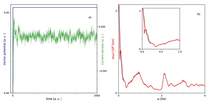
Figure 1: a) Sigmoidal pulse (blue) in the $z$ direction vs. time with the induced current density (green) along $z$ vs. time, b) dynamical electrical conductivity component $\sigma_{zz}$. The black dashed line is the Drude fit that yields the DC conductivity. The inset plot shows the dynamical electrical conductivity at low energies.

III Results

III.1 Equation of State

By employing ground-state DFT in conjunction with the Hubbard correction, we examine, as shown in Fig. 2, the EOS, the electronic density of states (DOS), and the phonon DOS of iron across a pressure range of approximately 180 GPa. In doing so, we specifically analyze the impact of electronic correlations on the EOS. In Fig. 2a), we present our findings (depicted as red and orange curves) alongside previous experimental measurements Boehler et al. (2008); Dewaele et al. (2006); Sakai et al. (2014); Fei et al. (2016); Ono et al. (2010) (denoted by black symbols) and theoretical predictions Pourovskii (2019); Sha and Cohen (2010); Zhuang et al. (2021); Sola, Brodholt, and Alfè (2009); Steinle-Neumann, Cohen, and Stixrude (2004) (denoted by green symbols). Our results are obtained by fitting total energies from DFT calculations using the PBE functional (GGA) Perdew, Burke, and Ernzerhof (1996) for various volumes to the Vinet EOS Vinet et al. (1987, 1989). The calculations with a Hubbard correction (+$U$) are also carried out for the spin-polarized case using the PBE functional around the mean-field form with double counting Czyżyk and Sawatzky (1994); Cococcioni and De Gironcoli (2005).

We first examine the equation of state (EOS) shown in Fig. 2a). In the BCC phase, the inclusion of the GGA$+U$ correction yields a relatively modest but notable improvement over the GGA functional alone. The GGA$+U$ calculations effectively shift the results towards a better agreement with the experimental findings reported by Dewaele et al.Dewaele et al. (2006). Moreover, our GGA$+U$ results are consistent with the findings obtained from LDA calculations augmented by dynamical mean field theory (DMFT) calculations, as reported by Pourvoskii et al.Pourovskii (2019). However, our findings suggest that employing a GGA functional alone is sufficient to reasonably capture the ground state properties Cococcioni and De Gironcoli (2005) of the ferromagnetic BCC phase, particularly when considering the significant static exchange splitting present in the system.

As pressure increases, the antiferromagnetic HCP phase becomes the stable phase Steinle-Neumann, Stixrude, and Cohen (2004); Cohen and Mukherjee (2004); Lizárraga et al. (2008); Thakor et al. (2003), starting at approximately 13 GPa (refer to Fig. 7 in Appendix A for the enthalpy curve). In this phase, electronic correlations play a more significant role as the static exchange splitting reduces bonding. Previous studies have considered these dynamical many-body effects using dynamical mean field theory (DMFT) to account for the impact of the +$U$ correction on the EOS Pourovskii et al. (2014).

In the HCP phase, we observe a similar trend to the BCC phase. At lower pressures, HCP iron exhibits strong correlation effects. While our results obtained using GGA agree well with available DFT and quantum Monte Carlo (QMC) data in the literature Sha and Cohen (2010); Zhuang et al. (2021); Sola, Brodholt, and Alfè (2009); Steinle-Neumann, Cohen, and Stixrude (2004), they visibly deviate from experimental measurements. Consequently, our GGA$+U$ calculations provide more accurate results and are in agreement with the LDA+DMFT results of Pourvoskii et al.Pourovskii (2019) in the pressure range of 13-30 GPa. However, even with the inclusion of the Hubbard correction to improve the treatment of strong correlations, the volume change in the EOS still deviates from experimental dataBoehler et al. (2008); Dewaele et al. (2006); Sakai et al. (2014); Fei et al. (2016); Ono et al. (2010) by approximately 5% at around 70 a.u.³/atom. The GGA predictions yield a $c/a$ ratio of less than 1.60, which further decreases with increasing volume Pourovskii et al. (2014), while DMFT predicts a nearly constant $c/a$ ratio of approximately 1.60 regardless of volume, consistent with experimental measurements Glazyrin et al. (2013); Dewaele et al. (2006). In the pressure range of 40-50 GPa, the correlation effects are slightly better captured by LDA+DMFT compared to GGA$+U$. At higher pressures (>100 GPa), our GGA results align well with experimental data Boehler et al. (2008); Dewaele et al. (2006); Sakai et al. (2014); Fei et al. (2016); Ono et al. (2010) and previous theoretical efforts Sha and Cohen (2011); Steinle-Neumann, Cohen, and Stixrude (2004); Zhuang et al. (2021) as the importance of correlations diminishes.

Fig. 2b) shows the spin-resolved DOS of HCP iron at high pressure computed using DFT and DFT+$U$. At relatively low pressure (17.7 GPa), DFT+$U$ results in substantial changes in the occupancy of the $3d$ electrons near the Fermi energy. The DOS in the HCP phase at ambient pressure computed using DFT+DMFT Hausoel et al. (2017) is additionally shown for reference. There is a striking resemblance in the peak feature above the Fermi energy between the DFT+$U$ and DMFT results, even though the DMFT results are calculated at ambient pressure.

Fig. 2c) shows the phonon DOS obtained via finite differences force constants as implemented in phonopy Togo et al. (2023); Togo (2023) at pressures of 71.5 GPa and 138 GPa. They agree with the experimental results obtained using nuclear resonant inelastic x-ray scattering (NRIXS) at pressures of 71 GPa and 136 GPa respectively Gleason, Mao, and Zhao (2013). The figure clearly demonstrates that the influence of the Hubbard correction on the phonon density of states (DOS) is insignificant within the considered pressure ranges, consistent with the available experimental data.

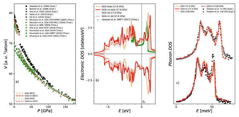
Figure 2: a) Equation of state (EOS) for BCC and HCP iron. Experimental data for ambient temperature (T=300 K) stems from Refs. Boehler et al., 2008; Dewaele et al., 2006; Sakai et al., 2014; Fei et al., 2016; Ono et al., 2010. Theoretical data at T=0 K and ambient temperature (T=300 K) stems from Refs. Pourovskii, 2019; Sha and Cohen, 2010; Zhuang et al., 2021; Sola, Brodholt, and Alfè, 2009; Steinle-Neumann, Cohen, and Stixrude, 2004, b) Spin-resolved density of states (DOS) of HCP iron at 17.6 GPa computed using DFT and DFT+$U$. Contribution from the 3d states is indicated by the dotted lines. HCP DOS at ambient pressure stems from Ref. Hausoel et al., 2017, c) Phonon density of states for HCP iron at 71.5 GPa (bottom) and 138 GPa (top) computed using DFT and DFT+$U$. Experimental data on HCP iron for pressures 71 GPa and 136 GPa at ambient temperature stems from Ref. Gleason, Mao, and Zhao, 2013.

III.2 Dynamical Conductivity

In the following, we investigate the impact of electronic correlation effects on the dynamical conductivity of iron in both the BCC and HCP phases.

III.2.1 BCC Iron

The frequency-dependent conductivity (Eq. 5) obtained using RT-TDDFT (red solid) including Hubbard corrections for BCC iron under ambient conditions is shown in Fig. 3. Due to the symmetry of the BCC lattice ($a=b=c$), it is sufficient to compute a single diagonal component of the conductivity tensor ($\sigma_{ab}$). In our case, we compute the $\sigma_{zz}$ component and compare our results with the KG results (green dashed) by Alfè et al. Alfè, Pozzo, and Desjarlais (2012), at a slightly elevated temperature (T=500 K), and experimental results by Paquain Paquin (1995), Palik Palik (1998) and Cahill Cahill et al. (2019) at ambient temperature. Overall, the RT-TDDFT results are in remarkable agreement with the experimental results by Paquain Paquin (1995) and Palik Palik (1998) throughout the considered frequency range, and with the experimental results by Cahill Cahill et al. (2019) at lower frequencies. In contrast, the KG method, widely regarded as the standard approach for computing electrical conductivities, falls short of providing an accurate description across the entire frequency domain. In not displaying the drop in conductivity up to $50$ eV, the KG method averages over the feature at $\sim$55 eV which stems from 3p to conduction band transitions.

The DC conductivities obtained from the KG method (9.03 $\mathrm{M}\mathrm{S}\mathrm{m}^{-1}$), extracted through a Drude-like fit using different k-point sampling and cell sizes Alfè, Pozzo, and Desjarlais (2012), exhibit values close to those reported in experimental studies ($\sim$10 $\mathrm{M}\mathrm{S}\mathrm{m}^{-1}$) Gomi et al. (2013); Seagle et al. (2013). Similarly, the DC conductivities derived from RT-TDDFT+U yield a value of 8.83 $\mathrm{M}\mathrm{S}\mathrm{m}^{-1}$, further confirming their consistency with experimental observations.

It is common to verify simulation data in terms of the f-sum rule Mahan (2013)

$$\frac{1}{\pi}\int_{0}^{\infty}d\omega\ \sigma(\omega)=n_{e},$$ (6)

where $n_{e}$ is the number of electrons in the simulation cell. Evaluated in a frequency range up to $\sim$5 Ha (i.e., $\sim$136 eV) and normalized to the f-sum rule of the experimental data by Paquin Paquin (1995), this yields ratio of 0.95 for RT-TDDFT compared to 0.97 using the KG formula obtained by Alfè et al. Alfè, Pozzo, and Desjarlais (2012) evaluated up to $\sim$5.5 Ha (i.e., $\sim$150 eV directly from the f-sum rule) providing a measure of the quality of our calculations.

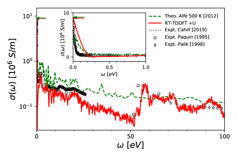
Figure 3: Dynamical electrical conductivity of BCC iron at ambient conditions computed using RT-TDDFT with Hubbard corrections. DC values for the RT-TDDFT (red) and KG (green) results are indicated by the arrows. The inset plot shows the dynamical electrical conductivity at low energies. Experimental data stems from Refs. Paquin, 1995; Cahill et al., 2019; Palik, 1998. Theoretical data at T=500 K evaluated using the Kubo-Greenwood formula stems from Ref. Alfè, Pozzo, and Desjarlais, 2012.

III.2.2 HCP Iron

In the HCP phase, we evaluate the conductivity tensor similar to the BCC phase discussed earlier but along various directions and analyze the corresponding tensor components. This is relevant because the asymmetrical HCP lattice ($a=b\neq c$), as opposed to the BCC lattice, requires the computation of additional tensor components and could be of great aid for characterizing materials exhibiting the Hall effect Hall et al. (1879); Elliott, Shallcross, and Sharma (2022). Fig. 4 shows the frequency-dependent conductivity of HCP iron at 23 GPa obtained using RT-TDDFT with Hubbard corrections along the $z$ ($\sigma_{zz}$ - red solid) and $x$ ($\sigma_{xx}$ - blue dashed) directions. Notably, no experimental or theoretical data exist for direct comparison under these conditions, making our study the first benchmark for future experiments in this domain.

The DC conductivities are represented by arrows, with the $z$ and $x$ directions yielding DC values ranging from 7.42 $\mathrm{M}\mathrm{S}\mathrm{m}^{-1}$ to 1.65 $\mathrm{M}\mathrm{S}\mathrm{m}^{-1}$, respectively. These values align with experimental resistivity (inverse of conductivity) measurements Seagle et al. (2013); Gomi et al. (2013). The significant anisotropy in the DC conductivity holds particular relevance for experiments conducted with diamond anvil cells (DAC), as crystallographic orientations play a vital role in determining the observed behavior.

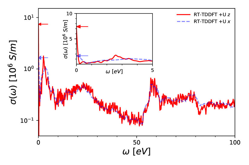
Figure 4: Dynamical electrical conductivity of HCP iron at 23 GPa computed using RT-TDDFT with Hubbard $U$ corrections along the $z$ (red) and $x$ (blue) directions. The inset plot shows the dynamical electrical conductivity at low energies. Anisotropy in the DC conductivity is inferred from the arrows.

III.3 DC Conductivity with Pressure

Now we turn to the DC conductivity evaluated using RT-TDDFT at high pressures. Fig. 5 shows the DC conductivity as a function of pressure in the BCC and HCP phases at ambient temperature (T=300 K). The results in the BCC phase are indicated by solid red circles and those in the HCP phase by empty red circles. In the BCC phase, our predicted DC conductivity is in the range reported by several experiments Yousuf, Sahu, and Rajan (1986); Gomi et al. (2013); Paquin (1995); Palik (1998). With increasing pressure in the BCC phase, the DC conductivity drops in agreement with the experiments Gomi et al. (2013); Seagle et al. (2013). There is a further drop in the conductivity observed near 13 GPa which marks the transition between the BCC and the HCP phase. Note that a similar drop in the conductivity during the phase transition has been observed for several other materials Balchan and Drickamer (1961); Garg, Vijayakumar, and Godwal (2004). In contrast to the experimental results Gomi et al. (2013); Seagle et al. (2013) and our results, ab initio calculations by Sha et al. Sha and Cohen (2011) report an increase in the conductivity for the BCC phase with pressure although the drop in the conductivity during the phase transition is captured. The discrepancies in the theoretical results can be attributed to the use of density functional perturbation theory (DFPT) by Sha et al. to evaluate the electrical resistivity, whereas our work employs the more effective approach of RT-TDDFT. By considering electronic correlations more accurately, as demonstrated earlier in the analysis of dynamical electrical conductivity, RT-TDDFT proves to be a superior method for capturing the relevant physics.

Our results in the HCP phase exhibit good agreement with experimental data from Seagle and Gomi et al.Seagle et al. (2013); Gomi et al. (2013), as well as with the findings of C. Zhang et al.Zhang et al. (2018) up to 50 GPa. Additionally, our results align well with the measurements on HCP iron by Y. Zhang et al.Zhang et al. (2020), as indicated by the black dotted line, particularly for pressures below 50 GPa. Notably, our results differ significantly from the calculations by Sha et al.Sha and Cohen (2011), as their estimations overestimate the conductivity in the HCP phase. The black dashed line represents the model-based pressure and temperature dependence of the resistivity, derived by Seagle et al.Seagle et al. (2013), which agrees well with our findings for pressures above 50 GPa.

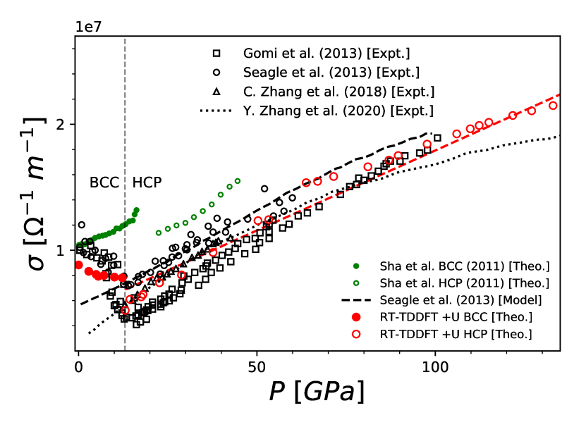
Figure 5: Pressure versus DC conductivity at ambient temperature (T=300 K). The results of this work are indicated by solid and empty red circles for BCC and HCP phases respectively. The drop in the electrical conductivity around $\sim$13 GPa indicates the BCC$\rightarrow$HCP phase transition. The red dashed line is the linear fit to our HCP data. The black dashed line is a pressure and temperature-based model by Seagle et al. Seagle et al. (2013). The black dotted line is the fitted results to the experimental measurements by Y. Zhang et al. Zhang et al. (2020). Theoretical data stems from Ref. Sha and Cohen, 2011. Experimental data stems from Refs. Gomi et al., 2013; Seagle et al., 2013; Zhang et al., 2018.

III.4 Thermal Conductivity in HCP Iron with Pressure

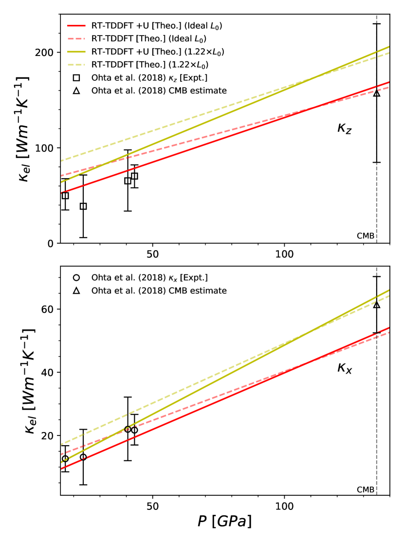
Figure 6: Electronic components of the thermal conductivity of HCP iron along different directions (top panel - $z$ direction, bottom panel - $x$ direction) vs pressure. The inclusion of Hubbard corrections ($+U$) is additionally shown. The dashed and the solid lines are the linear fit to RT-TDDFT and RT-TDDFT+$U$ results respectively. The red and the yellow curves shown are computed using the ideal Lorenz number ($L_{0}$) and 1.22$\times L_{0}$ respectively. Experimental anisotropy data (black hollow squares and black hollow circles) at ambient temperature (T=300 K) stems from Ref. Ohta et al., 2018. Estimated data (black hollow triangles) at the core-mantle boundary (CMB) conditions from Ref. Ohta et al., 2018.

Finally, we analyze the electronic component of the thermal conductivity of HCP iron along the $z$ (top panel) and $x$ (bottom panel) directions, as depicted in Fig. 6. The thermal conductivity is determined from the electrical conductivity using the Wiedemann-Franz law Franz and Wiedemann (1853). Given the pressure and temperature conditions in this study, we expect the Wiedemann-Franz law to be valid, as both energy and charge transport is predominantly governed by the same free carriers, with inelastic scattering effects becoming less significant. For our calculations, we employ the ideal Lorenz number ($L_{0}$=2.44$\times 10^{-8}$ W$\Omega$K^-2), as well as an experimentally determined Lorenz number (1.22$\times L_{0}$) established by Secco et al.Secco (2017) under ambient conditions, for comparison. It is worth noting that the conventional Lorenz number used under high-pressure and high-temperature conditions exhibits substantial variations across previous studies Pozzo et al. (2012); de Koker, Steinle-Neumann, and Vlček (2012); Pozzo et al. (2014); Ohta et al. (2016); Konôpková et al. (2016); Xu et al. (2018).

Our findings exhibit excellent agreement with the experimental data obtained from laser-heated diamond anvil cell (DAC) measurements conducted by Ohta et al.Ohta et al. (2018) (depicted as black hollow squares and black hollow circles for $\kappa_{z}$ and $\kappa_{x}$, respectively) at pressures below 50 GPa. Notably, the Hubbard corrections play a crucial role, particularly at lower pressures where electronic correlations are more pronounced. Neglecting the Hubbard corrections leads to a deviation of up to 40$\%$ along the $z$ direction around 13 GPa. We extend our calculations to the pressure regime encountered at the core-mantle boundary (CMB) in Earth’s interior (P$\sim$135 GPa). Here, we additionally present the estimated thermal conductivity (depicted as black hollow triangles) by Ohta Ohta et al. (2018). At CMB conditions, we report a $\kappa_{z}/\kappa_{x}$ ratio of 3.03, which is comparable to the value of $2.56\pm 0.48$ estimated by Ohta et al.Ohta et al. (2018). The thermal conductivity of pure iron at CMB conditions is estimated by Seagle et al.Seagle et al. (2013) to be 145 Wm^-1K^-1. Our predictions fall within this range, with a value of $158.4$ Wm^-1K^-1 ($197.4$ Wm^-1K^-1 when considering 1.22$\times L_{0}$), aligning with previous theoretical effortsde Koker, Steinle-Neumann, and Vlček (2012); Pozzo et al. (2012). Taking the trace average of the conductivity tensor $\sum_{i=(x,y,z)}\sigma_{ii}/3$ into account, the resulting thermal conductivity near CMB conditions (P$\sim$135GPa) is approximately 87 Wm^-1K^-1 (approximately 109 Wm^-1K^-1 when considering 1.22$\times L_{0}$). This analysis emphasizes the impact of electronic correlations on thermal conductivity at pressures up to 50 GPa, underscoring the importance of employing the RT-TDDFT methodology with Hubbard corrections for accurate simulation and modeling.

In recent studies, the total thermal conductivity, accounting, in addition, for the coupling between phonons and magnons, has been split into various contributions, as demonstrated by Nikolov et al.Nikolov et al. (2022). Their work highlights the significant contribution of the electronic component (approximately 80-90$\%$) at ambient temperatureBäcklund (1961); Wu, Liu, and Luo (2018). For the purpose of this study, we have thus focused solely on the electronic contribution to thermal conductivity. Experimental measurements of ferromagnetic BCC iron at ambient conditions show a total thermal conductivity of 77.3 Wm^-1K^-1, with the electronic contribution estimated at 69.4 Wm^-1K^-1 according to the Wiedemann-Franz law Fulkerson, Moore, and McElroy (1966). In comparison, our calculations yield a thermal conductivity of 64.6 Wm^-1K^-1 (78.6 Wm^-1K^-1 using 1.22$\times L_{0}$) according to the Wiedemann-Franz law.

IV Conclusions

In this study, we comprehensively investigated the influence of electronic correlations on various properties of solid iron at high pressures. These properties include ground state characteristics such as the EOS, the electronic DOS, and the phonon DOS, as well as electronic transport properties including electrical and thermal conductivity. To perform our analysis, we employed RT-TDDFT with Hubbard corrections and compared the results with those obtained using the conventional KG method for transport properties.

Our findings clearly demonstrate that electronic correlation effects have a significant impact on the investigated properties up to pressures of 50 GPa Pourovskii et al. (2014). Moreover, our work highlights the advantages of utilizing RT-TDDFT (including Hubbard corrections) as a more reliable method for computing electronic transport properties compared to the current state-of-the-art approach, such as the KG method.

We envision promising applications of this methodology in studying structural phase transitions and spin response Kaa et al. (2022) in materials under extreme conditions, made possible by recent advancements in free-electron lasers Zastrau et al. (2021); Cerantola et al. (2021). The frequency-dependent electrical conductivity, along with the analysis of anisotropy in HCP iron, can serve as a valuable benchmark for future experiments, particularly in the context of advanced diagnostics.

Furthermore, the role of magnetism in iron-nickel alloys under Earth-core conditions has been shown to be significant, highlighting the importance of electronic correlations, which were previously assumed to be negligible Vekilova et al. (2015); Hausoel et al. (2017). In the future, incorporating electronic correlations into the ab initio analysis of electronic transport properties in the liquid phase of iron and iron alloys relevant to Earth-core conditions would be an important task to pursue.

Data Availability

The data that support the findings of this study are available from the corresponding author upon reasonable request.

Appendix A Appendix

A comparison between the calculated lattice constant, magnetic moment, and bulk modulus within several approximate DFT schemes, ab initio methods, and experimental results are shown in Table. 1.

Table 1: Comparison between the calculated lattice constant, magnetic moment, and bulk modulus within several approximate DFT schemes, experimental and theoretical results for BCC iron.

Method	$a_{0}$ (a.u.)	$\mu_{0}$ ($\mu_{b}$)	$B_{0}$ (GPa)
Spin-pol. LDA	5.21	2.02	259
Spin-pol. PBEsol	5.28	2.09	213
Spin-pol. PBE	5.37	2.19	169
Spin-pol. PBE+$U$	5.39	-	166
Spin-pol. LDAa	5.20	1.95	-
Spin-pol. LDA+$U^{a}$	5.35	2.73	-
Spin-pol. PBEsola	5.35	2.12	-
Spin-pol. PBEsol+$U^{a}$	5.35	2.71	-
Spin-pol. PBEa	5.20	2.19	-
Spin-pol. PBE+$U^{a}$	5.37	2.09	-
Spin-pol. LDAe	5.22	2.33	210
LDA+DMFTf	5.39	-	172
Expt.	5.42b	2.22c	173d

Fig. 7 shows the variation of enthalpy with pressure for the BCC and HCP phases of iron. The inset plot indicates the relative difference in enthalpy between the phases with the phase transition occurring at $\sim$12.9 GPa in agreement with the range observed in experiments Bancroft, Peterson, and Minshall (1956); Takahashi and Bassett (1964).

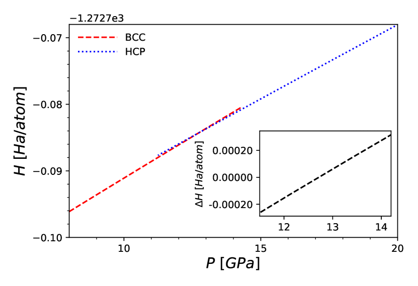
Figure 7: Enthalpy versus pressure for BCC and HCP phases of iron. The inset plot shows the relative difference in enthalpy ($\Delta H_{BCC}-\Delta H_{HCP}$) between the phases versus pressure.

References

- Anderson (1986) O. L. Anderson, “Properties of iron at the earth’s core conditions,” Geophysical Journal International 84, 561–579 (1986).
- Mao, Bassett, and Takahashi (1967) H. Mao, W. A. Bassett, and T. Takahashi, “Effect of pressure on crystal structure and lattice parameters of iron up to 300 kbar,” Journal of Applied Physics 38, 272–276 (1967).
- Anzellini et al. (2013) S. Anzellini, A. Dewaele, M. Mezouar, P. Loubeyre, and G. Morard, “Melting of iron at earth’s inner core boundary based on fast x-ray diffraction,” Science 340, 464–466 (2013).
- Kraus et al. (2022) R. G. Kraus, R. J. Hemley, S. J. Ali, J. L. Belof, L. X. Benedict, J. Bernier, D. Braun, R. Cohen, G. W. Collins, F. Coppari, et al., “Measuring the melting curve of iron at super-earth core conditions,” Science 375, 202–205 (2022).
- Kuwayama et al. (2008) Y. Kuwayama, K. Hirose, N. Sata, and Y. Ohishi, “Phase relations of iron and iron–nickel alloys up to 300 GPa: Implications for composition and structure of the earth’s inner core,” Earth and Planetary Science Letters 273, 379–385 (2008).
- Tateno et al. (2010) S. Tateno, K. Hirose, Y. Ohishi, and Y. Tatsumi, “The structure of iron in earth’s inner core,” Science 330, 359–361 (2010).
- Dewaele et al. (2006) A. Dewaele, P. Loubeyre, F. Occelli, M. Mezouar, P. I. Dorogokupets, and M. Torrent, “Quasihydrostatic equation of state of iron above 2 Mbar,” Phys. Rev. Lett. 97, 215504 (2006).
- Mao et al. (1990) H. Mao, Y. Wu, L. Chen, J. Shu, and A. P. Jephcoat, “Static compression of iron to 300 GPa and \ceFe_0.8Ni_0.2 alloy to 260 GPa: Implications for composition of the core,” Journal of Geophysical Research: Solid Earth 95, 21737–21742 (1990).
- Zhang, Johansson, and Vitos (2011) H. Zhang, B. Johansson, and L. Vitos, “Density-functional study of paramagnetic iron,” Physical Review B 84, 140411 (2011).
- Bancroft, Peterson, and Minshall (1956) D. Bancroft, E. L. Peterson, and S. Minshall, “Polymorphism of iron at high pressure,” Journal of Applied Physics 27, 291–298 (1956).
- Takahashi and Bassett (1964) T. Takahashi and W. A. Bassett, “High-pressure polymorph of iron,” Science 145, 483–486 (1964).
- Mathon et al. (2004) O. Mathon, F. Baudelet, J. P. Itié, A. Polian, M. d’Astuto, J. C. Chervin, and S. Pascarelli, “Dynamics of the magnetic and structural phase transition in iron,” Phys. Rev. Lett. 93, 255503 (2004).
- Iota et al. (2007) V. Iota, J.-H. P. Klepeis, C.-S. Yoo, J. Lang, D. Haskel, and G. Srajer, “Electronic structure and magnetism in compressed 3d transition metals,” Applied Physics Letters 90, 042505 (2007).
- Hohenberg and Kohn (1964) P. Hohenberg and W. Kohn, “Inhomogeneous electron gas,” Phys. Rev. 136, B864–B871 (1964).
- Kohn and Sham (1965) W. Kohn and L. J. Sham, “Self-consistent equations including exchange and correlation effects,” Phys. Rev. 140, A1133–A1138 (1965).
- Anisimov, Aryasetiawan, and Lichtenstein (1997) V. I. Anisimov, F. Aryasetiawan, and A. Lichtenstein, “First-principles calculations of the electronic structure and spectra of strongly correlated systems: the LDA+ U method,” Journal of Physics: Condensed Matter 9, 767 (1997).
- Cococcioni and De Gironcoli (2005) M. Cococcioni and S. De Gironcoli, “Linear response approach to the calculation of the effective interaction parameters in the LDA+ U method,” Physical Review B 71, 035105 (2005).
- Kotliar et al. (2006) G. Kotliar, S. Y. Savrasov, K. Haule, V. S. Oudovenko, O. Parcollet, and C. A. Marianetti, “Electronic structure calculations with dynamical mean-field theory,” Rev. Mod. Phys. 78, 865–951 (2006).
- Paul and Birol (2019) A. Paul and T. Birol, “Applications of dft+ dmft in materials science,” Annual Review of Materials Research 49, 31–52 (2019).
- Sánchez-Barriga et al. (2009) J. Sánchez-Barriga, J. Fink, V. Boni, I. Di Marco, J. Braun, J. Minár, A. Varykhalov, O. Rader, V. Bellini, F. Manghi, et al., “Strength of correlation effects in the electronic structure of iron,” Physical review letters 103, 267203 (2009).
- Sponza et al. (2017) L. Sponza, P. Pisanti, A. Vishina, D. Pashov, C. Weber, M. Van Schilfgaarde, S. Acharya, J. Vidal, and G. Kotliar, “Self-energies in itinerant magnets: a focus on \ceFe and \ceNi,” Physical Review B 95, 041112 (2017).
- Kubo (1957) R. Kubo, “Statistical-mechanical theory of irreversible processes. i. general theory and simple applications to magnetic and conduction problems,” Journal of the Physical Society of Japan 12, 570–586 (1957).
- Greenwood (1958) D. A. Greenwood, “The boltzmann equation in the theory of electrical conduction in metals,” Proceedings of the Physical Society 71, 585–596 (1958).
- Desjarlais, Kress, and Collins (2002) M. P. Desjarlais, J. D. Kress, and L. A. Collins, “Electrical conductivity for warm, dense aluminum plasmas and liquids,” Phys. Rev. E 66, 025401 (2002).
- Witte et al. (2017) B. B. L. Witte, L. B. Fletcher, E. Galtier, E. Gamboa, H. J. Lee, U. Zastrau, R. Redmer, S. H. Glenzer, and P. Sperling, “Warm dense matter demonstrating non-drude conductivity from observations of nonlinear plasmon damping,” Phys. Rev. Lett. 118, 225001 (2017).
- Schörner et al. (2022) M. Schörner, B. B. L. Witte, A. D. Baczewski, A. Cangi, and R. Redmer, “Ab initio study of shock-compressed copper,” Phys. Rev. B 106, 054304 (2022).
- Pozzo, Desjarlais, and Alfè (2011) M. Pozzo, M. P. Desjarlais, and D. Alfè, “Electrical and thermal conductivity of liquid sodium from first-principles calculations,” Phys. Rev. B 84, 054203 (2011).
- de Koker, Steinle-Neumann, and Vlček (2012) N. de Koker, G. Steinle-Neumann, and V. Vlček, “Electrical resistivity and thermal conductivity of liquid Fe alloys at high P and T, and heat flux in earth’s core,” Proceedings of the National Academy of Sciences 109, 4070–4073 (2012).
- Vlček, De Koker, and Steinle-Neumann (2012) V. Vlček, N. De Koker, and G. Steinle-Neumann, “Electrical and thermal conductivity of Al liquid at high pressures and temperatures from ab initio computations,” Physical Review B 85, 184201 (2012).
- Korell et al. (2019) J.-A. Korell, M. French, G. Steinle-Neumann, and R. Redmer, “Paramagnetic-to-diamagnetic transition in dense liquid iron and its influence on electronic transport properties,” Phys. Rev. Lett. 122, 086601 (2019).
- French and Mattsson (2014) M. French and T. R. Mattsson, “Thermoelectric transport properties of molybdenum from simulations,” Phys. Rev. B 90, 165113 (2014).
- Kleinschmidt et al. (2023) U. Kleinschmidt, M. French, G. Steinle-Neumann, and R. Redmer, “Electrical and thermal conductivity of fcc and hcp iron under conditions of the earth’s core from ab initio simulations,” Phys. Rev. B 107, 085145 (2023).
- Pourovskii et al. (2017) L. Pourovskii, J. Mravlje, A. Georges, S. Simak, and I. Abrikosov, “Electron–electron scattering and thermal conductivity of -iron at earth’s core conditions,” New Journal of Physics 19, 073022 (2017).
- Cazzaniga et al. (2011) M. Cazzaniga, H.-C. Weissker, S. Huotari, T. Pylkkänen, P. Salvestrini, G. Monaco, G. Onida, and L. Reining, “Dynamical response function in sodium and aluminum from time-dependent density-functional theory,” Phys. Rev. B 84, 075109 (2011).
- Ramakrishna et al. (2021) K. Ramakrishna, A. Cangi, T. Dornheim, A. Baczewski, and J. Vorberger, “First-principles modeling of plasmons in aluminum under ambient and extreme conditions,” Phys. Rev. B 103, 125118 (2021).
- Yabana and Bertsch (1996) K. Yabana and G. F. Bertsch, “Time-dependent local-density approximation in real time,” Phys. Rev. B 54, 4484–4487 (1996).
- Baczewski et al. (2016) A. D. Baczewski, L. Shulenburger, M. Desjarlais, S. Hansen, and R. Magyar, “X-ray thomson scattering in warm dense matter without the chihara decomposition,” Physical review letters 116, 115004 (2016).
- Baczewski et al. (2021) A. D. Baczewski, T. Hentschel, A. Kononov, and S. B. Hansen, “Predictions of bound-bound transition signatures in x-ray thomson scattering,” (2021), arXiv:2109.09576 .
- Ramakrishna et al. (2023) K. Ramakrishna, M. Lokamani, A. Baczewski, J. Vorberger, and A. Cangi, “Electrical conductivity of iron in earth’s core from microscopic ohm’s law,” Phys. Rev. B 107, 115131 (2023).
- Dornheim et al. (2023) T. Dornheim, Z. A. Moldabekov, K. Ramakrishna, P. Tolias, A. D. Baczewski, D. Kraus, T. R. Preston, D. A. Chapman, M. P. Böhme, T. Döppner, F. Graziani, M. Bonitz, A. Cangi, and J. Vorberger, “Electronic density response of warm dense matter,” Physics of Plasmas 30 (2023).
- Ohta et al. (2018) K. Ohta, Y. Nishihara, Y. Sato, K. Hirose, T. Yagi, S. I. Kawaguchi, N. Hirao, and Y. Ohishi, “An experimental examination of thermal conductivity anisotropy in hcp iron,” Frontiers in Earth Science , 176 (2018).
- et al. (2023) J. K. D. et al., “Elk, all-electron full-potential linearised augmented plane wave (fp-lapw) code,” http://elk.sourceforge.net (2023).
- Vekilova et al. (2015) O. Y. Vekilova, L. Pourovskii, I. Abrikosov, and S. Simak, “Electronic correlations in fe at earth’s inner core conditions: Effects of alloying with ni,” Physical Review B 91, 245116 (2015).
- Hausoel et al. (2017) A. Hausoel, M. Karolak, E. Şaşoğlu, A. Lichtenstein, K. Held, A. Katanin, A. Toschi, and G. Sangiovanni, “Local magnetic moments in iron and nickel at ambient and earth’s core conditions,” Nature communications 8, 1–9 (2017).
- Glazyrin et al. (2013) K. Glazyrin, L. V. Pourovskii, L. Dubrovinsky, O. Narygina, C. McCammon, B. Hewener, V. Schünemann, J. Wolny, K. Muffler, A. I. Chumakov, W. Crichton, M. Hanfland, V. B. Prakapenka, F. Tasnádi, M. Ekholm, M. Aichhorn, V. Vildosola, A. V. Ruban, M. I. Katsnelson, and I. A. Abrikosov, “Importance of correlation effects in hcp iron revealed by a pressure-induced electronic topological transition,” Phys. Rev. Lett. 110, 117206 (2013).
- Steinle-Neumann, Stixrude, and Cohen (2004) G. Steinle-Neumann, L. Stixrude, and R. E. Cohen, “Magnetism in dense hexagonal iron,” Proceedings of the National Academy of Sciences 101, 33–36 (2004).
- Steinle-Neumann, Cohen, and Stixrude (2004) G. Steinle-Neumann, R. Cohen, and L. Stixrude, “Magnetism in iron as a function of pressure,” Journal of Physics: Condensed Matter 16, S1109 (2004).
- Perdew, Burke, and Ernzerhof (1996) J. P. Perdew, K. Burke, and M. Ernzerhof, “Generalized gradient approximation made simple,” Physical review letters 77, 3865 (1996).
- Petukhov et al. (2003) A. Petukhov, I. Mazin, L. Chioncel, and A. Lichtenstein, “Correlated metals and the LDA+ U method,” Physical Review B 67, 153106 (2003).
- Czyżyk and Sawatzky (1994) M. T. Czyżyk and G. A. Sawatzky, “Local-density functional and on-site correlations: The electronic structure of \ceLa_2CuO_4 and \ceLaCuO_3,” Phys. Rev. B 49, 14211–14228 (1994).
- Mohammed et al. (2010) Y. S. Mohammed, Y. Yan, H. Wang, K. Li, and X. Du, “Stability of ferromagnetism in Fe, Co, and Ni metals under high pressure with GGA and GGA+ U,” Journal of magnetism and magnetic materials 322, 653–657 (2010).
- Vignale and Kohn (1996) G. Vignale and W. Kohn, “Current-dependent exchange-correlation potential for dynamical linear response theory,” Physical review letters 77, 2037 (1996).
- Vignale, Ullrich, and Conti (1997) G. Vignale, C. A. Ullrich, and S. Conti, “Time-dependent density functional theory beyond the adiabatic local density approximation,” Physical review letters 79, 4878 (1997).
- Boehler et al. (2008) R. Boehler, D. Santamaría-Pérez, D. Errandonea, and M. Mezouar, “Melting, density, and anisotropy of iron at core conditions: New x-ray measurements to 150 GPa,” Journal of Physics: Conference Series 121, 022018 (2008).
- Sakai et al. (2014) T. Sakai, S. Takahashi, N. Nishitani, I. Mashino, E. Ohtani, and N. Hirao, “Equation of state of pure iron and \ceFe_0.9Ni_0.1 alloy up to 3 Mbar,” Physics of the Earth and Planetary Interiors 228, 114–126 (2014).
- Fei et al. (2016) Y. Fei, C. Murphy, Y. Shibazaki, A. Shahar, and H. Huang, “Thermal equation of state of hcp-iron: Constraint on the density deficit of earth’s solid inner core,” Geophysical Research Letters 43, 6837–6843 (2016).
- Ono et al. (2010) S. Ono, T. Kikegawa, N. Hirao, and K. Mibe, “High-pressure magnetic transition in hcp-Fe,” American Mineralogist 95, 880–883 (2010).
- Pourovskii (2019) L. V. Pourovskii, “Electronic correlations in dense iron: from moderate pressure to earth’s core conditions,” Journal of Physics: Condensed Matter 31, 373001 (2019).
- Sha and Cohen (2010) X. Sha and R. E. Cohen, “First-principles thermal equation of state and thermoelasticity of hcp Fe at high pressures,” Phys. Rev. B 81, 094105 (2010).
- Zhuang et al. (2021) J. Zhuang, H. Wang, Q. Zhang, and R. M. Wentzcovitch, “Thermodynamic properties of -Fe with thermal electronic excitation effects on vibrational spectra,” Physical Review B 103, 144102 (2021).
- Sola, Brodholt, and Alfè (2009) E. Sola, J. P. Brodholt, and D. Alfè, “Equation of state of hexagonal closed packed iron under earth’s core conditions from quantum monte carlo calculations,” Phys. Rev. B 79, 024107 (2009).
- Vinet et al. (1987) P. Vinet, J. R. Smith, J. Ferrante, and J. H. Rose, “Temperature effects on the universal equation of state of solids,” Physical Review B 35, 1945 (1987).
- Vinet et al. (1989) P. Vinet, J. H. Rose, J. Ferrante, and J. R. Smith, “Universal features of the equation of state of solids,” Journal of Physics: Condensed Matter 1, 1941 (1989).
- Cohen and Mukherjee (2004) R. Cohen and S. Mukherjee, “Non-collinear magnetism in iron at high pressures,” Physics of the Earth and Planetary Interiors 143, 445–453 (2004).
- Lizárraga et al. (2008) R. Lizárraga, L. Nordström, O. Eriksson, and J. Wills, “Noncollinear magnetism in the high-pressure hcp phase of iron,” Physical Review B 78, 064410 (2008).
- Thakor et al. (2003) V. Thakor, J. B. Staunton, J. Poulter, S. Ostanin, B. Ginatempo, and E. Bruno, “Ab initio calculations of incommensurate antiferromagnetic spin fluctuations in hcp iron under pressure,” Phys. Rev. B 67, 180405 (2003).
- Pourovskii et al. (2014) L. V. Pourovskii, J. Mravlje, M. Ferrero, O. Parcollet, and I. A. Abrikosov, “Impact of electronic correlations on the equation of state and transport in -Fe,” Phys. Rev. B 90, 155120 (2014).
- Sha and Cohen (2011) X. Sha and R. Cohen, “First-principles studies of electrical resistivity of iron under pressure,” Journal of Physics: Condensed Matter 23, 075401 (2011).
- Togo et al. (2023) A. Togo, L. Chaput, T. Tadano, and I. Tanaka, “Implementation strategies in phonopy and phono3py,” J. Phys. Condens. Matter 35, 353001 (2023).
- Togo (2023) A. Togo, “First-principles phonon calculations with phonopy and phono3py,” J. Phys. Soc. Jpn. 92, 012001 (2023).
- Gleason, Mao, and Zhao (2013) A. Gleason, W. Mao, and J. Zhao, “Sound velocities for hexagonally close-packed iron compressed hydrostatically to 136 GPa from phonon density of states,” Geophysical Research Letters 40, 2983–2987 (2013).
- Alfè, Pozzo, and Desjarlais (2012) D. Alfè, M. Pozzo, and M. P. Desjarlais, “Lattice electrical resistivity of magnetic bcc iron from first-principles calculations,” Physical Review B 85, 024102 (2012).
- Paquin (1995) R. A. Paquin, “Properties of metals,” Handbook of optics 2, 35–49 (1995).
- Palik (1998) E. D. Palik, Handbook of optical constants of solids, Vol. 3 (Academic press, 1998).
- Cahill et al. (2019) J. T. Cahill, D. T. Blewett, N. V. Nguyen, A. Boosalis, S. J. Lawrence, and B. W. Denevi, “Optical constants of iron and nickel metal and an assessment of their relative influences on silicate mixture spectra from the FUV to the NIR,” Icarus 317, 229–241 (2019).
- Gomi et al. (2013) H. Gomi, K. Ohta, K. Hirose, S. Labrosse, R. Caracas, M. J. Verstraete, and J. W. Hernlund, “The high conductivity of iron and thermal evolution of the earth’s core,” Physics of the Earth and Planetary Interiors 224, 88–103 (2013).
- Seagle et al. (2013) C. T. Seagle, E. Cottrell, Y. Fei, D. R. Hummer, and V. B. Prakapenka, “Electrical and thermal transport properties of iron and iron-silicon alloy at high pressure,” Geophysical Research Letters 40, 5377–5381 (2013).
- Mahan (2013) G. D. Mahan, Many-particle physics (Springer Science & Business Media, 2013).
- Hall et al. (1879) E. H. Hall et al., “On a new action of the magnet on electric currents,” American Journal of Mathematics 2, 287–292 (1879).
- Elliott, Shallcross, and Sharma (2022) P. Elliott, S. Shallcross, and S. Sharma, “The giant spin hall effect at optical frequencies,” (2022), arXiv:2204.01538 .
- Yousuf, Sahu, and Rajan (1986) M. Yousuf, P. C. Sahu, and K. G. Rajan, “High-pressure and high-temperature electrical resistivity of ferromagnetic transition metals: Nickel and iron,” Physical Review B 34, 8086 (1986).
- Balchan and Drickamer (1961) A. Balchan and H. Drickamer, “High pressure electrical resistance cell, and calibration points above 100 kilobars,” Review of Scientific Instruments 32, 308–313 (1961).
- Garg, Vijayakumar, and Godwal (2004) A. B. Garg, V. Vijayakumar, and B. Godwal, “Electrical resistance measurements in a diamond anvil cell to 40 GPa on ytterbium,” Review of scientific instruments 75, 2475–2478 (2004).
- Zhang et al. (2018) C. Zhang, J.-F. Lin, Y. Liu, S. Feng, C. Jin, M. Hou, and T. Yoshino, “Electrical resistivity of fe-c alloy at high pressure: Effects of carbon as a light element on the thermal conductivity of the earth’s core,” Journal of Geophysical Research: Solid Earth 123, 3564–3577 (2018).
- Zhang et al. (2020) Y. Zhang, M. Hou, G. Liu, C. Zhang, V. B. Prakapenka, E. Greenberg, Y. Fei, R. E. Cohen, and J.-F. Lin, “Reconciliation of experiments and theory on transport properties of iron and the geodynamo,” Phys. Rev. Lett. 125, 078501 (2020).
- Franz and Wiedemann (1853) R. Franz and G. Wiedemann, “Ueber die wärme-leitungsfähigkeit der metalle,” Annalen der Physik 165, 497–531 (1853).
- Secco (2017) R. A. Secco, “Thermal conductivity and seebeck coefficient of Fe and Fe-Si alloys: Implications for variable lorenz number,” Physics of the Earth and Planetary Interiors 265, 23–34 (2017).
- Pozzo et al. (2012) M. Pozzo, C. Davies, D. Gubbins, and D. Alfè, “Thermal and electrical conductivity of iron at earth’s core conditions,” Nature 485, 355–358 (2012).
- Pozzo et al. (2014) M. Pozzo, C. Davies, D. Gubbins, and D. Alfè, “Thermal and electrical conductivity of solid iron and iron–silicon mixtures at earth’s core conditions,” Earth and Planetary Science Letters 393, 159–164 (2014).
- Ohta et al. (2016) K. Ohta, Y. Kuwayama, K. Hirose, K. Shimizu, and Y. Ohishi, “Experimental determination of the electrical resistivity of iron at earth’s core conditions,” Nature 534, 95–98 (2016).
- Konôpková et al. (2016) Z. Konôpková, R. S. McWilliams, N. Gómez-Pérez, and A. F. Goncharov, “Direct measurement of thermal conductivity in solid iron at planetary core conditions,” Nature 534, 99–101 (2016).
- Xu et al. (2018) J. Xu, P. Zhang, K. Haule, J. Minar, S. Wimmer, H. Ebert, and R. E. Cohen, “Thermal conductivity and electrical resistivity of solid iron at earth’s core conditions from first principles,” Phys. Rev. Lett. 121, 096601 (2018).
- Nikolov et al. (2022) S. Nikolov, J. Tranchida, K. Ramakrishna, M. Lokamani, A. Cangi, and M. Wood, “Dissociating the phononic, magnetic and electronic contributions to thermal conductivity: a computational study in alpha-iron,” Journal of Materials Science , 1–14 (2022).
- Bäcklund (1961) N. Bäcklund, “An experimental investigation of the electrical and thermal conductivity of iron and some dilute iron alloys at temperatures above 100 K,” Journal of Physics and Chemistry of Solids 20, 1–16 (1961).
- Wu, Liu, and Luo (2018) X. Wu, Z. Liu, and T. Luo, “Magnon and phonon dispersion, lifetime, and thermal conductivity of iron from spin-lattice dynamics simulations,” Journal of Applied Physics 123, 085109 (2018).
- Fulkerson, Moore, and McElroy (1966) W. Fulkerson, J. Moore, and D. McElroy, “Comparison of the thermal conductivity, electrical resistivity, and seebeck coefficient of a high-purity iron and an armco iron to 1000° \ceC,” Journal of Applied Physics 37, 2639–2653 (1966).
- Kaa et al. (2022) J. M. Kaa, C. Sternemann, K. Appel, V. Cerantola, T. R. Preston, C. Albers, M. Elbers, L. Libon, M. Makita, A. Pelka, et al., “Structural and electron spin state changes in an x-ray heated iron carbonate system at the earth’s lower mantle pressures,” Physical Review Research 4, 033042 (2022).
- Zastrau et al. (2021) U. Zastrau, K. Appel, C. Baehtz, O. Baehr, L. Batchelor, A. Berghäuser, M. Banjafar, E. Brambrink, V. Cerantola, T. E. Cowan, et al., “The high energy density scientific instrument at the european xfel,” Journal of synchrotron radiation 28 (2021).
- Cerantola et al. (2021) V. Cerantola, A. D. Rosa, Z. Konôpková, R. Torchio, E. Brambrink, A. Rack, U. Zastrau, and S. Pascarelli, “New frontiers in extreme conditions science at synchrotrons and free electron lasers,” Journal of Physics: Condensed Matter 33, 274003 (2021).
- Tavadze et al. (2021) P. Tavadze, R. Boucher, G. Avendaño-Franco, K. X. Kocan, S. Singh, V. Dovale-Farelo, W. Ibarra-Hernández, M. B. Johnson, D. S. Mebane, and A. H. Romero, “Exploring DFT+ U parameter space with a bayesian calibration assisted by markov chain monte carlo sampling,” npj Computational Materials 7, 1–9 (2021).
- Chiarotti (1995) G. Chiarotti, “1.6 crystal structures and bulk lattice parameters of materials quoted in the volume,” in Physics of Solid Surfaces · Structure (Springer, 1995) pp. 21–26.
- Kikuchi, Suzuki, and Katayama (1990) H. Kikuchi, Y. Suzuki, and T. Katayama, “Structure and magnetic properties of single-crystal Fe/Au (100) superlattices synthesized using RHEED oscillation,” Journal of applied physics 67, 5403–5405 (1990).
- Adams et al. (2006) J. J. Adams, D. Agosta, R. Leisure, and H. Ledbetter, “Elastic constants of monocrystal iron from 3 to 500 K,” Journal of applied physics 100, 113530 (2006).