Absence of localization in two-dimensional Clifford circuits

Abstract

We analyze a Floquet circuit with random Clifford gates in one and two spatial dimensions. By using random graphs and methods from percolation theory, we prove in the two dimensional setting that some local operators grow at ballistic rate, which implies the absence of localization. In contrast, the one-dimensional model displays a strong form of localization characterized by the emergence of left and right-blocking walls in random locations. We provide additional insights by complementing our analytical results with numerical simulations of operator spreading and entanglement growth, which show the absence (presence) of localization in two-dimension (one-dimension). Furthermore, we unveil that the spectral form factor of the Floquet unitary in two-dimensional circuits behaves like that of quasi-free fermions with chaotic single particle dynamics, with an exponential ramp that persists till times scaling linearly with the size of the system. Our work sheds light on the nature of disordered, Floquet Clifford dynamics and its relationship to fully chaotic quantum dynamics.

I Introduction

Understanding the dynamics of quantum many-body systems far from equilibrium is of fundamental importance for preparing and controlling quantum states of matter [1]. The universal dynamical behavior provide signatures of novel quantum phase of matter and their underlying patterns of quantum information. Studying the dynamics of quantum many-body systems is notoriously challenging due to the exponential growth of the Hilbert space. In recent years, simulating dynamics in a quantum circuit architecture has opened new directions for probing quantum chaos, hydrodynamics, and non-equilibrium phases of matter [2, 3, 4, 5, 6, 7, 8, 9]. They are particularly suitable for quantum simulation on noisy intermediate-scale quantum (NISQ) devices and have been studied on the state-of-the-art physical platforms. Novel quantum many-body phenomena can be realised in these experiments providing a test bed for the theoretical ideas with potential applications in protecting and processing quantum information.

The dynamics in circuit models are encoded in the form of k-local unitary gates acting on qubits. The geometry of the gates and their symmetries provide access to a wide range of model phenomena which are analytically tractable and can be approximated efficiently. Due to their tunability and control, circuit models provide minimal models for complex quantum phenomena, including systems with kinetic constraints [10, 11], dual-unitary structure [12, 13], periodic dynamics [14], or long-range interactions [15]. Notably, quantum circuits with random gates have provided a powerful framework to strive for a quantum computational advantage [16] as well as to study quantum information scrambling on existing quantum hardware [17].

The vast majority of many-body quantum systems are ergodic and relax to thermal equilibrium under unitary time evolution [18, 19]. Exceptions to this generic thermalizing behavior include integrable models [20], which possess an extensive set of conservation laws, as well as models exhibiting localization [21, 22]. Localization can arise in systems with sufficiently strong disorder, and one of its signatures is the slow growth of any initially-local operator when evolving in the Heisenberg picture. In a quantum circuit, localization in terms of operator growth can be of single-particle type, where the support of any initially local operator remains confined in a finite region for all times [23, 24], as realized for instance in lattice models of non-interacting fermions with random on-site potential [25] and for the corresponding mapping to spin-systems [26, 27]. For a typical realization of our circuit in one dimension, this definition takes into account the appearance of walls that block the spread of any operator, like illustrated in Fig. 1 (a). On the other hand, many-body localization exhibits the growth of support of a local operator as the logarithm of time [28]. In particular the log-like growth of entanglement entropy in time [29, 30, 31] tells these systems apart from the Anderson-type localized as defined below in definition 1. In one-dimensional systems, a many-body localized phase with an extensive set of exponentially localized integrals of motion might exist at sufficiently strong disorder [32]. However, the asymptotic existence of this MBL phase in the thermodynamic limit is still under active debate as localization has recently been found to be unstable even at rather large values of disorder [33, 34, 35, 36, 37]. Moreover, in higher dimensions, analytical arguments and numerical calculations suggest that MBL is unstable [38, 39, 40, 41, 42, 43].

Disorder in quantum circuit models can be introduced in space and time where the gates are chosen at random. Random unitary dynamics without any symmetries or constraints lead to complete mixing [3, 4, 44, 45] while certain time-periodic circuits can exhibit non-ergodic dynamics [14, 46]. There are also various forms of kinetically constrained random circuits, akin to fractonic models, which exhibit localization [47, 48]. In this work we shed light on the role of dimensionality on localization in random Floquet Clifford circuits. Floquet circuits have been extensively studied [49, 50, 51, 52, 53, 46] and have provided key insights into the properties of periodically-driven quantum systems [54]. They have been essential to rigorously demonstrate the occurrence of chaos and random-matrix behavior in isolated quantum systems [49, 52] and, in combination with disorder and many-body localization, they can host exotic non-equilibrium phases of matter with no equilibrium counterpart [55, 56]. Moreover, certain circuits with dual-unitary structure allow for a controlled tuning between ergodic and non-ergodic dynamics [13, 12]. In this work, we analytically and numerically study absence of localization in two-dimensional Clifford circuits and characterise the integrable nature of chaos using measures of operator growth and spectral form factor. Moreover we numerically contrast the two-dimensional against the one-dimensional case showing for the latter localization at the dynamical level.

From a quantum information perspective, the Clifford group plays a key role in fault-tolerant quantum computing and randomized benchmarking [57, 58, 59]. Recently, random circuits consisting of Clifford gates have provided useful insights into quantum many-body physics [2, 60, 14, 61, 62] due to their efficient simulability on classical computers despite the generation of extensive amounts of entanglement. This efficient simulability of Clifford dynamics can also be understood in terms of a phase space representation analogous to that of quasi-free bosons and fermions, with the dimension of the phase space being exponentially smaller than the Hilbert space, see appendix A of [14] and [63, 64]. Yet, Clifford circuits form unitary designs [65, 66, 67] such that circuit averages of certain relevant quantities can exactly reproduce Haar averages over the full unitary group. Despite their simplicity, Clifford circuits can thus prove useful to gain insights into some aspects of the dynamics of more generic quantum systems, including the buildup of out-of-time-ordered correlators or the growth of entanglement [3, 4].

In addition, as we will demonstrate, the Clifford circuits studied in this paper are to some extent tractable analytically by a suitable mapping to directed graphs. It is known that random time-dependent (i.e. annealed disorder) cellular automata can be analysed with directed-percolation theory [68, 69], and that Clifford circuits can be represented as cellular automata. However, the circuits considered by us are not random in time, they have quench disorder, and hence, they cannot in general be solved with directed graphs. Nevertheless, as we will show below, in order to probe their behaviour, we only need to analyse the dynamics at the edge of the light-cone. Moreover, at the light-cone edge, spatial disorder is equivalent to time disorder, producing an effectively annealed dynamics, which can be analysed with percolation theory.

The hybrid nature of Clifford circuits between integrable and chaotic systems also reflects itself in the emergence of ergodicity and localization. On one hand, it was shown in Ref. [14], that Floquet Clifford circuits exhibit Anderson-type localization in one dimension (1D), cf. Fig. 1 (a) and definition 1. On the other hand, we prove here, and numerically show cf. Fig. 1 (b), as a main result, that in two dimensions (2D) some operators always grow at ballistic rate such that the model does not localize, despite having strong disorder, contrasting the phenomenon in one dimension. We also provide numerical evidence that the ballistic growth happens for almost all local operators. Moreover, the absence of localization in our time-periodic 2D circuit model differs from the behavior of disordered free-fermion models which show Anderson localization for arbitrarily weak disorder in 2D [70, 71, 72].

We elucidate further aspects of the Floquet Clifford dynamics by complementing our analytical results with numerical simulations, where we demonstrate that operator spreading is exponentially suppressed in 1D, reminiscent of the exponential dynamical-localization of the wave function in Anderson insulators. On the contrary, we find that operator spreading in 2D occurs ballistically with light-speed velocity and that the interior of the light-cone becomes fully scrambled and featureless. These findings are substantiated by the temporal buildup of entanglement, which is bounded and system-size independent in 1D, whereas it grows linearly and saturates towards extensive values in 2D. Finally, we also study the spectral form factor (SFF) of the Floquet Clifford circuit, which is a key quantity to diagnose the emergence of quantum chaos. We show that the SFF is similar to that of free fermions whose associated single-particle dynamics is chaotic. Specifically, we find that, in the 2D model, the SFF exhibits an exponential ramp at early times that persists up to a time that scales linearly with the size of the system, suggesting that ergodicity in the case of Clifford dynamics should be understood with respect to the exponentially smaller phase space.

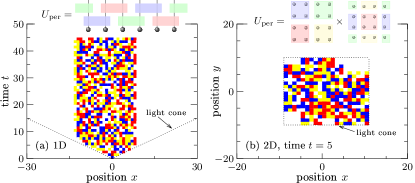
Figure 1: Localization and its absence in Floquet Clifford circuits. A local operator $\sigma_{x}$ acting non-trivially only on a single site evolves according to a time-periodic Clifford circuit in (a) one dimension and (b) two dimensions. In 1D, the Floquet unitary $U_{\text{per}}$ consists of a brickwork pattern of 2-qubit gates, while in 2D it consists of two layers of 4-qubit gates, cf. Fig. 2. The color plot encodes the local matrices of the time-evolved operator string $U(t)\sigma_{x}U^{\dagger}(t)$ according to $\mathbbm{1}$ (white), $\sigma_{x}$ (blue), $\sigma_{y}$ (red), $\sigma_{z}$ (yellow). Data is shown for a single random realization of the Clifford gates. For better visualization of the 2D data, we focus in panel (b) on a single point in time, $t=5$, where the light cone boundary (dotted square) is of size $20\times 20$, cf. definition 2. As proven in Ref. [14], the 1D circuit exhibits localization due to the emergence of left- and right-sided walls that confine the evolution at all times. This confinement affects all (not necessarily Pauli) operators with support between the two walls. Inside the confined region the evolution looks ergodic. In contrast, in 2D, localization is absent as can be seen from the fact that parts of the operator grow with light-cone speed.

Our work provides a comprehensive picture of localization and chaos in disorderd, Floquet Clifford quantum-circuits, in terms of directed percolation, at the light-cone, and information spreading in classical cellular automata. Understanding of non-equilibrium quantum many-body states in Clifford circuits provides an important starting point for studying the phenomena in generic conditions. It can serve as a useful benchmark for identifying quantum effects of simulation in noisy quantum devices. The relevance of Clifford circuits for quantum error-correction can also provide valuable insights into combining error-correction protocols with quantum simulation.

The rest of this paper is structured as follows. Section II.1 contains a description of the model, including the definition of Clifford unitaries, which are the building blocks of this quantum circuit. Section II.2 contains the main result of our work, theorem 4, together with a discussion of its significance, as well as its numerical demonstration in Sec. II.3. In Sec. II.4, we numerically study the spectral form factor of Floquet Clifford unitaries which supports our observation of localization in 1D, see also [14], and ergodic dynamics in 2D. We also provide a rigorous lower bound on the time-averaged spectral form factor. Section III contains the proof of theorem 4, which uses random graphs and methods reminiscent of those of percolation theory. Eventually, in Sec. IV, we provide a discussion about the fact that Clifford dynamics appears to share properties of integrable systems and chaotic systems, Sec. V summarizes the results of this work and provides some outlook. Appendix A provides the relation among localization length and the average position of a blocking wall in the dynamics of the one-dimension model.

II Results

II.1 Description of the model

Consider an infinite two-dimensional square lattice with sites labeled by $(x,y)\in\mathbb{Z}^{2}$. In each site there is a spin-1/2 particle, or qubit, which has Hilbert space $\mathbb{C}^{2}$. The dynamics of the system is time-periodic, with the period being one unit of time. Hence, at integer times $t\in\mathbb{Z}$, the evolution operator can be written as $U(t)=(U_{\text{per}})^{t}$. The unitary $U_{\text{per}}$ that describes the dynamics of a single period has the form

$$U_{\text{per}}=\left(\bigotimes_{x,y\text{ odd}}W_{(x,y)}\right)\left(\bigotimes_{x,y\text{ even}}W_{(x,y)}\right),$$ (1)

where, for any $(x,y)\in\mathbb{Z}^{2}$, the local unitary $W_{(x,y)}$ acts on the four sites $(x,y)$, $(x+1,y)$, $(x,y+1)$ and $(x+1,y+1)$. In (1), $(x,y\text{ odd})$ means that both $x$ and $y$ are odd, analogously $(x,y\text{ even})$ means that both $x$ and $y$ are even. In the dynamics described by (1) each time period decomposes into two half time-steps, which are illustrated in Fig. 2. This quantum circuit with local interactions is an example of a quantum cellular automaton [73, 74, 75, 11]. The evolution operator $U(t)$ can also be generated by a time-periodic Hamiltonian $H(t)$ with local interactions

$$U(t)=\mathcal{T}e^{-\mathrm{i}\int_{0}^{t}d\tau H(\tau)}\ ,$$ (2)

where $\mathcal{T}$ stands for time-ordered exponential. This type of dynamics is called Floquet dynamics [54].

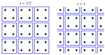
Figure 2: Local dynamics. This figure represents the two layers of local unitaries generating the dynamics of a time period $U_{\text{per}}$. Each black dot represents a qubit and each blue square represents a four-qubit unitary $W_{(x,y)}$.

The disorder of the system is represented by the fact that each local unitary $W_{(x,y)}$ is sampled independently from the uniform distribution over the 4-qubit Clifford group. A unitary $W$ is Clifford if it maps any product of Pauli sigma matrices to another product of Pauli sigma matrices [63, 76]. An example of Clifford unitary $W$ acting on $\mathbb{C}^{2}\otimes\mathbb{C}^{2}$ is

$$W(\sigma_{x}\otimes\mathbbm{1})W^{\dagger} =\sigma_{z}\otimes\sigma_{x}\ ,$$ (3)

$$W(\sigma_{z}\otimes\mathbbm{1})W^{\dagger} =\mathbbm{1}\otimes\sigma_{z}\ ,$$ (4)

$$W(\mathbbm{1}\otimes\sigma_{x})W^{\dagger} =\sigma_{z}\otimes\mathbbm{1}\ ,$$ (5)

$$W(\mathbbm{1}\otimes\sigma_{z})W^{\dagger} =\sigma_{x}\otimes\sigma_{z}\ .$$ (6)

It can be seen that this four identities fully specify $W$ up to a global phase. Clearly, having random Clifford unitaries in neighboring unit cells is a somewhat different type of disorder than the one usually considered in the study of localization (e.g., random on-site magnetic fields in spin-chain models [21, 22]). For instance, apart from the fact that the unitaries are drawn independently, it is not immediately obvious how to quantify the strength of disorder in the random circuit model.

In summary, we have an ensemble of models of which we are going to study the typical behaviour. Note that, while the statistics defining the model is translation invariant, typical instances are not. This approach is standard in the study of disorder and localization [23]. We also have to mention that the Floquet Clifford circuit described in Eq. (1) and Fig. 2 is a straightforward 2D version of the 1D model considered in [14]. Remarkably, in Ref. [14] it was proven that the 1D Floquet model with 2-qubit Clifford gates acting in a brickwork pattern supports Anderson-type localization. More specifically, initially-local operators remain confined to a finite region in space during the time evolution due to the emergence of left and right-sided walls, cf. Fig. 1 (a), that confine the operator spreading at all times, see also [77]. Here, we will proof that this kind of localization is absent in the 2D model, cf. Fig. 1 (b). In this context, let us note that this absence of localization in 2D is in contrast to the results of Ref. [77], which studied similar Floquet Clifford circuits hosting a localization-delocalization transition in 2D. However, while Ref. [77] considered a drastically reduced gate set (only two different two-qubit Clifford elements), our circuits are more general with gates being drawn at random from the full Clifford group.

One difference between the 1D [Fig. 1 (a)] and the 2D model [Fig. 1 (b)] is that in the former case the gates are sampled from the 2-qubit Clifford group ${\cal C}_{2}$, while in the latter case they are sampled from the 4-qubit Clifford group ${\cal C}_{4}$. Both contain a finite number of distinct elements, but their dimensions differ substantially, i.e., $|{\cal C}_{2}|=11520$ and $|{\cal C}_{4}|\approx 1.2\times 10^{13}$ [78].

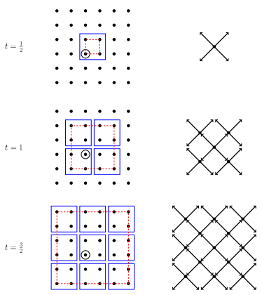
Figure 3: Light-cone boundary growth. The left column shows the light-cone and its boundary at times $t\in\{1/2,1,3/2\}$ of an operator acting on the encircled site at $t=0$. Black dots represent sites, blue squares represent four-qubit unitaries and the red dashed line is the light-cone boundary. The right column shows the piece of the directed graph $G$ which describes the growth history of the boundary up to the corresponding time $t$. Each vertex in $G$ represents a unitary and each arrow represents a qubit at a particular time $t$. The arrows which do not point to any vertex represent the qubits of the boundary at time $t$.

In the following, our analytical arguments will be focused on the 2D model (1) and we refer the interested reader to Ref. [14] for the proof of localization in 1D. However, in order to provide a concrete comparison of their properties, we will present numerical results of operator spreading and entanglement growth (Sec. II.3), as well as simulations of the spectral form factor (Sec. II.4), for both 1D and 2D Floquet Clifford circuits.

II.2 Absence of localization

Many-body lattice systems display localization when the Lieb-Robinson velocity vanishes. Next we provide a definition of Anderson-type localization based on [26].

Definition 1.

Let $O^{H}(t)=e^{iHt}Oe^{-iHt}$ be the evolution in the Heisenberg picture of a local observable $O$ with support at the origin of the lattice, and let $O^{H}_{l}(t)$ be the restriction of $O^{H}(t)$ onto the ball of radius $l>0$ around the origin. A system displays Anderson-type localization if there are parameters $c,\mu>0$ such that

$$\underset{H}{\mathbb{E}}\sup_{t}\|O^{H}_{l}(t)-O^{H}(t)\|_{\infty}\leq c\,e^{-\frac{l}{\mu}}\ ,$$ (7)

for all $l>0$. (The operator norm $\|A\|_{\infty}$ is the spectral radius of $A$, that for finite systems is the largest singular value of $A$.)

Note that the left-hand side of (7) involves an average over all realisations of the dynamics $H$, which usually correspond to different realisations of a random potential. In the case of QCAs or Floquet systems, the average is taken over the single-period unitary $U_{\text{per}}$ characterising the dynamics $O(t)=U_{\text{per}}^{-t}HU_{\text{per}}^{t}$. In particular, in quantum circuits, the average runs over all realizations of the circuit. The above definition implies that, if a system has a dynamics such that a local operator grows at linear rate (ballistically) in some direction, then we can conclude that there is no localization of any type. With this in mind we make the following definitions.

Definition 2.

The light-cone is the largest support that a single-site operator at $t=0$ could have at each future time $t$ when we maximize over instances of the dynamics (see figure 3). At each time $t$, the boundary of the light-cone consists of the outer qubits contained in the light-cone, which form a square of side $4t$.

The approximate shape of the light-cone is a four-sided pyramid, the apex of which is the site where the initial operator is supported. The surface of this pyramid is the boundary of the light-cone. In general, an operator may not have full support inside the light-cone, because it acts as the identity in some sites at particular times (see figure 4). However, despite not having full support, an operator may grow at maximal speed, as defined next.

Definition 3.

A model has light-speed operator growth if there is a single-site operator whose evolution has non-trivial support (is non-identity) on the boundary of the light-cone at all future times $t=1,2,3,\ldots$ (see figure 4).

Figure 4: Light-speed growth. In this example, an operator located at the circled site at time $t=0$ evolves into an operator with support on the blue sites at time $t=1$. Since some of this blue sites are at the light-cone boundary (red dashed line) this operator enjoys light-speed growth (at least up to time $t=1$).

Light-speed operator growth implies absence of localization. However, not having light-speed operator growth does not imply localization. For example, ballistic growth at a rate smaller than unity is not localization. Also, diffusive dynamics, where the diameter of the support of an operator grows like the square root of time is not localization. In what follows we introduce the main result of this work, which establishes the absence of localization in our model.

Theorem 4.

Consider a Pauli operator which differs from the identity only on a single site at $t=0$. With probability at least $0.44$, the time evolution of this operator generated by the random dynamics (1) is non-identity on some sites of the boundary of the light-cone at all times $t\in\{1/2,1,3/2,2,5/2,\ldots\}$.

That is, with probability 0.44, a particular Pauli operator at a particular site enjoys light-speed growth. Our numerical simulations strongly suggests that this happens for a fraction much larger than 0.44. Non-Pauli operators are more prone to light-speed growth, because they have more than one term when expressed in the Pauli basis, and hence more likelihood that at least one term has light-speed growth.

Before turning to the formal proof of theorem 4 in Sec. III, we now provide numerical support for the presence (absence) of localization in 1D (2D) random Floquet Clifford circuits. In particular, let us note that while some aspects of the Clifford dynamics can be treated analytically (cf. Sec. III), others are accessible only by numerical means.

II.3 Numerical analysis of Floquet Clifford circuits

II.3.1 Simulating Clifford circuits

Clifford circuits can be efficiently simulated on classical computers by exploiting the stabilizer formalism [63, 64]. More specifically, a stabilizer state $\ket{\psi}$ on $L$ qubits can be uniquely defined by $L$ operators ${\cal P}_{i}$ according to ${\cal P}_{i}\ket{\psi}=\ket{\psi}$, where the ${\cal P}_{i}$ are $L$-qubit Pauli strings. Instead of keeping track of the time evolution of the quantum state directly, $\ket{\psi}\to U(t)\ket{\psi}$, it is then useful to consider the evolution of the operators, ${\cal P}_{i}\to U(t){\cal P}_{i}U^{\dagger}(t)$. The latter can be done efficiently if $U(t)$ consists solely of Clifford gates which map single Pauli strings to other single Pauli strings, cf. Eq. (3), in stark contrast to more general quantum evolution which would yield superpositions of multiple Pauli strings. More specifically, the $L$ stabilizers ${\cal P}_{i}$ can be encoded in a $L\times 2L$ binary matrix, also called the stabilizer tableau, the values of which are updated suitably upon the application of a Clifford gate. As a consequence, the time and memory requirements scale only polynomially with the number of qubits, see Ref. [63] for further details. In fact, time-evolving the entire stabilizer tableau of a state $\ket{\psi}$ will here be necessary only for calculating the entanglement entropy in Fig. 6, whereas the analysis of operator spreading (Figs. 1 and 5) and of the spectral form factor below (Fig. 7) requires the evolution of single (or, in case of the SFF, a specific set of) operators. Eventually, we note that there exist various efficient algorithms to generate random elements of the Clifford group [78, 79]. We here follow the approach of Ref. [80], which we use to sample uniformly from ${\cal C}_{2}$ (${\cal C}_{4}$) in our simulations of 1D (2D) circuit geometries. Except for Fig. 1, we then present results that are averaged over a sufficient number of random circuit realizations.

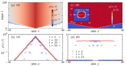
Figure 5: Operator spreading. Circuit-averaged $\rho(x,t)$ in 1D [panels (a),(b)] and 2D [panels (c),(d)]. Data is obtained by time evolving an initially local operator $\sigma_{x}$ located at the origin, and averaging over $\sim 10^{4}$ random circuit realizations. Panels (b) and (d) show cuts of the data in (a) and (c) at fixed times $t$. For the better visualization of the 2D data, panel (c) shows $\rho(x,t)$ along a cut with $y=0$ [as indicated by the white arrow in the inset of panel (c), which depicts the full 2D data at $t=10$]. While in 1D, the operator becomes exponentially localized, with $\rho(x,t)\propto e^{-\frac{x}{\mu}}$ and $\mu\approx 10.4$, the operator grows with light speed in 2D with a maximally scrambled light-cone interior as indicated by $\rho(x,t)\approx 3/4$.

II.3.2 Operator spreading

Figure 1 (a) demonstrates the occurrence of localization in 1D Floquet Clifford circuits. Specifically, considering ${\cal O}(0)=\mathbbm{1}\otimes\cdots\otimes\mathbbm{1}\otimes\sigma_{x}\otimes\mathbbm{1}\otimes\cdots\otimes\mathbbm{1}$, that differs from the identity only on one site, Fig. 1 shows its time-evolution ${\cal O}(t)=U(t){\cal O}(0)U^{\dagger}(t)$ for a single random circuit realization. While the operator grows at light speed at short times, this growth eventually stops in 1D due to the emergence of left and right-blocking walls, leading to the Anderson-type localization behavior proven in Ref. [14]. In contrast, this kind of localization is absent in the 2D circuit [Fig. 1 (b)], where we find that at least some parts of the time-evolved operator grow with light speed, that is, they act nontrivially on the light-cone boundary at all times.

In order to study this operator spreading in more detail, let ${\cal O}_{x}(t)$ denote the local Pauli matrix at the $x$-th position of the time-evolved operator. (For example, given a two-qubit system and ${\cal O}(t)=\sigma_{x}\otimes\sigma_{z}$, we might have ${\cal O}_{1}(t)=\sigma_{x}$ and ${\cal O}_{2}(t)=\sigma_{z}$.) We then define the quantity $\rho(x,t)$, with

$$\rho(x,t)=\begin{cases}1\ ,\ &\text{if}\ {\cal O}_{x}(t)=\sigma_{x},\sigma_{y},\sigma_{z}\\ 0\ ,\ &\text{if}\ {\cal O}_{x}(t)=\mathbbm{1}\end{cases}\ ,$$ (8)

In Fig. 5, we show the circuit-averaged dynamics of $\rho(x,t)$ for 1D and 2D circuits. (Note that we here refrain from introducing another symbol for the average.) On one hand, in the case of 1D circuits [Fig. 5 (a),(b)], we find that most of the operator’s support remains close to the origin. More specifically, we find that the operator spreading is exponentially localized, with $\rho(x,t)\propto e^{-\frac{x}{\mu}}$, $\mu\approx 10.4$, and becomes essentially stationary at long times, as can be seen by comparing the cuts of $\rho(x,t)$ at times $t=25$ and $t=50$ in Fig. 5 (b).

On the other hand, the situation is clearly different in 2D [Fig. 5 (c),(d)]. In this case, we find that $\rho(x,t)$ is essentially featureless inside the light cone with $\rho(x,t)\approx 3/4$, with a sharp drop to $\rho(x,t)\to 0$ outside the light cone. Note that for better visualization, the data in Fig. 5 (c) is shown for a cut at $y=0$ of the original 2D data, cf. inset in 5 (c). Importantly, the circuit-averaged value $\rho(x,t)\approx 3/4$ indicates maximally scrambling dynamics. Namely, given the definition (8) of $\rho(x,t)$ above, this value indicates that the matrices $\sigma_{x},\sigma_{y},\sigma_{z}$, and $\mathbbm{1}$ locally occur all with equal probability.

It is in principle conceivable that there exist rare instances of random gate configurations such that the operator spreading becomes localized also in 2D. In practice, however, we do not observe any such localized instances and, in particular, there are no notable signatures in the circuit-averaged behavior of $\rho(x,t)$ in Fig. 5 (c) and (d).

II.3.3 Entanglement dynamics

To proceed, we now turn to the buildup of entanglement $S(t)$ between two parts $A$ and $B$ of the system, starting from an initially unentangled product state $\ket{\uparrow}^{\otimes L}$ stabilized by $\sigma_{z}$ everywhere. Within the stabilizer formalism, $S(t)$ can be efficiently simulated based on the collective evolution of all $L$ operators ${\cal P}_{i}$ that define $\ket{\psi}$ [2, 81]. Note that the entanglement dynamics in Clifford circuits is somewhat special since, given the reduced density matrix $\rho_{A}(t)=\text{tr}_{B}\ket{\psi(t)}\!\!\bra{\psi(t)}$, $\rho_{A}(t)$ will exhibit a flat eigenvalue spectrum such that all its Rényi entropies are equivalent [82]. Nevertheless, Clifford circuits can support extensive amounts of entanglement and the dynamics of $S(t)$ are often found to mimic the properties of more generic quantum evolutions [60, 15].

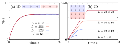
Figure 6: Entanglement growth. Half-system (cf. sketches) entanglement entropy $S(t)$ under Floquet Clifford evolution for different system sizes $L$ in (a) one dimension and (b) two dimensions. In 1D, $S(t)$ approaches an almost system-size independent long-time value. In 2D, $S(t)$ saturates towards the maximally achievable value $L/2$. [Note the different scales of the y-axis in (a) and (b).] Data are averaged over $\sim 10^{3}$ random circuit realizations.

In Fig. 6, we show $S(t)$ for half-system bipartitions in 1D and 2D Floquet Clifford circuits with various systems sizes $L$. The dynamics of $S(t)$ substantiate our previous observation of localization in 1D and ergodic behavior in 2D. Specifically, we find that $S(t)$ saturates towards a rather small and essentially $L$-independent long-time value $S(t\to\infty)\approx 10$ in 1D [Fig. 6 (a)]. This emphasizes that the localization length in 1D is distinctly shorter than the full system size and that a local operator can only explore a small part of the system, cf. Fig. 1 (a). In contrast, in 2D [Fig. 6 (b)], we find that $S(t)$ exhibits a pronounced linear increase at short times, well-known from other random-circuit models and chaotic quantum systems. Moreover, at longer times, $S(t)$ saturates towards an extensive long-time value $S(t\to\infty)\approx L/2$, which is the maximally achievable value for a system of size $L$. This volume-law scaling of $S(t)$ highlights the absence of localization in 2D Floquet Clifford circuits.

II.4 Spectral form factor

II.4.1 Definition and general remarks

To provide further insights into the nature of Floquet Clifford circuits we now turn to the SFF. The SFF of an ensemble of unitaries $\mathcal{U}$ is defined as

$$K(t)=\left\langle|\text{tr}\,U^{t}|^{2}\right\rangle\ ,$$ (9)

where $t$ takes integer values and the brackets $\langle\cdots\rangle$ denote average over all $U\in\mathcal{U}$. The SFF probes the statistical properties of the spectrum of randomly sampled unitaries in $\mathcal{U}$. In particular, the Fourier transform

$$\tilde{K}(\omega)=\frac{1}{\pi}\sum_{t=1}^{\infty}K(t)\,\cos(\omega t)\ ,$$ (10)

is the probability that a random $U\in\mathcal{U}$ has two eigenvalues separated by a distance $\omega$ (see [83]). The SFF also has an interpretation in terms of Poincaré recurrences, in fact $K(t)$ is a lower bound to the number of Pauli strings $\mathcal{P}$ which are mapped to themselves $U^{-t}\mathcal{P}U^{t}=\mathcal{P}$ after evolving for a time $t$. More precisely, it was proven in [84] that

$$K(t)=2^{-L}\sum_{\mathcal{P}}\left\langle\text{tr}\!\left[\mathcal{P}U^{-t}\mathcal{P}U^{t}\right]\right\rangle\ ,$$ (11)

where the sum is over all Pauli strings $\mathcal{P}$. This identity holds for any unitary $U$, although only Clifford unitaries have the property that $U^{-t}\mathcal{P}U^{t}$ is equal or orthogonal to $\pm\mathcal{P}$. The possibility of this negative sign is responsible for the fact that (11) is not necessarily equal to the number of recurrences, but a lower bound.

The SFF has been studied extensively to explore the onset of RMT behavior in the spectral properties of quantum systems [85, 86, 87, 50, 49]. In particular, it is proven in [83] that, for unitaries drawn from the uniform distribution (Haar measure) over SU$(2^{L})$, the SFF reads

$$K(t)=\left\{\begin{array}[]{ll}2^{2L}&\mbox{ if }t=0\\ t&\mbox{ if }1\leq t\leq 2^{L}\\ 2^{L}&\mbox{ if }t\geq 2^{L}\\ \end{array}\right..$$ (15)

Haar distributed unitaries go also under the name of CUE, circular unitary ensemble. Equation (15) shows that the SFF increases as a linear ramp before reaching a plateau. Many-body chaotic systems are defined such that their SFF increase linearly in time after an initial dip. The time at which the linear ramp starts is called Thouless time, the time at which the SFF reaches a plateau is called Heisenberg time. A meaningful interpretation of these time scales requires rescaling, as discussed for example in [88, 35]. Fig. 7 shows that the SFF of the periodic Clifford circuit that we are considering manifests an exponential ramp before reaching a plateau. A similar behavior is shown by quasi-free fermions with chaotic single-particle dynamics [89, 90]. (By quasi-free fermions we mean those having a Hamiltonian quadratic in the creation and annihilation operators.) Time in Fig. 7 is not rescaled and the value at which a plateau is reached is “evaluated” by inspection therefore we call it plateau-time instead of Heisenberg time.

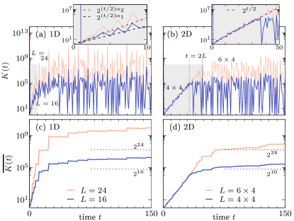
Figure 7: Spectral form factor. Circuit-averaged $K(t)$ of Floquet Clifford unitaries for different system sizes $L$ in (a) one dimension and (b) two dimensions. Data is averaged over $\sim 10^{6}$ random circuit realizations. The vertical dotted lines in (b) denote $t=2L$, which approximately marks the end of the exponential ramp. The insets in (a) and (b) show the same data, but now for shorter times, cf. shaded areas in (a) and (b). In 2D, we find that the ramp is described by $K(t)\propto 2^{t/2}$, while in 1D $K(t)\propto 2^{(t/2)\alpha}$ with $\alpha\approx 2.5$ for $L=16$ and $\alpha\approx 3.6$ for $L=24$. In all cases, $K(t=0)=4^{L}$. Panels (c) and (d) show the time-averaged SFF $\overline{K(t)}$ [Eq. 17] for 1D and 2D. The horizontal dashed lines indicate the Hilbert-space dimension $2^{L}$.

Building on the Clifford formalism it is possible to compute Eq. (11) efficiently [84], without explicitly evaluating the exponentially many terms. In order to do so, for any given Clifford unitary $U$, we define the group $H[U]$ of Pauli strings $\mathcal{P}$ that are invariant under the action of the unitary $U^{\dagger}\mathcal{P}U\pm\mathcal{P}$. Then, the method in [84] consists of finding a set of generators of the group $H[U]$, denoted $\text{gen}H[U]$, and exploit the following identity

$$|\text{tr}U|^{2}=\begin{cases}2^{|\text{gen}H[U]|}&\mbox{if }U^{\dagger}{\cal P}U=+{\cal P},\ \forall{\cal P}\in\text{gen}H[U]\\ 0&\text{otherwise}\end{cases}.$$

Then, this is done for $U=U_{\text{per}}^{t}$, with $U_{\text{per}}$ as defined in (1), and several values of $t$. Finally, one needs to average over many realizations of the circuit $U_{\text{per}}^{t}$. The exponential dependence of $K(t)$ on the number of generators already hints at the fact that the SFF in Clifford circuits will exhibit strong fluctuations.

II.4.2 Numerical results

We now present our numerical results for the SFF in Floquet Clifford unitaries. Note that while the stabilizer formalism in principle allows for simulations of $U(t)$ with complexity scaling polynomially with $L$, the system sizes in the following are smaller than one is typically used to from other examples of Clifford numerics. The main reason for this is that computing $K(t)$ requires averaging over a rather high number of circuit realizations, which makes simulations of larger $L$ quite costly. Especially for 2D circuits, we find that extensive averaging is required to obtain converging results since the calculation of $K(t)$ appears to be dominated by rare circuit realizations that yield very large values of $|\text{tr}U_{\text{per}}^{t}|^{2}$.

Figures 7 (a) and (b) show $K(t)$ for 1D and 2D circuits with two different system sizes $L=16,24$. For the 1D circuit, we find that $K(t)$ exhibits a steep exponential increase at early times, but quickly crosses over to a plateau-like behavior. The time at which this crossover takes place seems independent of $L$. Strikingly, however, this “plateau” is dominated by major fluctuations of the SFF. Note that (most of) these fluctuations are actual features of the dynamics of $K(t)$ and cannot be reduced further by circuit-averaging. In fact, the data in Fig. 7 are already averaged over a substantial number ($\sim 10^{6}$) of random realizations. These fluctuations follow from the fact that the Clifford group has finite cardinality $|\mathcal{C}_{L}|$, which implies that the length $t$ of the orbits (i.e. the smallest $t$ such that $U^{-t}\mathcal{P}U^{t}=\mathcal{P}$) are divisors of $|\mathcal{C}_{L}|$. To see this we recall Lagrange’s theorem: the order of a subgroup divides the order of the group. In particular, the smallest $r$ such that $U^{r}=\mathbbm{1}$ divides $|\mathcal{C}_{L}|$. Next, let us show that $t$ is divisor of $r$ (and consequently divisor of $|\mathcal{C}_{L}|$). If we assume the opposite then $r=nt+m$ with $0\leq m<t$, which implies $\mathcal{P}=U^{-r}\mathcal{P}U^{r}=U^{-m}\mathcal{P}U^{m}$, which contradicts the fact that $t$ is minimal.

The behavior of $K(t)$ changes notably in the case of 2D circuits [Fig. 7 (b)]. Similar to 1D, we again find an exponential increase of $K(t)$ at early times. However, in contrast to 1D, this ramp is cleaner and persists for a longer time in 2D. Specifically, comparing $K(t)$ for different $L$, we find that the end of the ramp occurs at $t_{\text{H}}\approx 2L$, which corresponds to the phase-space dimension of the Clifford dynamics, cf. Sec. IV.1. For times $t>2L$, the SFF displays strong fluctuations around the plateau value. We interpret this behavior of $K(t)$ as a signature of ergodic dynamics in phase space, analogous to quasi-free fermions, as discussed above.

Let us explain why in the 2D case the plateau-time grows with the system’s size as $t_{\text{H}}\approx 2L$ while in the 1D case $t_{\text{H}}$ is independent of $L$. Equation (11) tells us that $K(t)$ reaches the plateau when evolving Pauli strings experience recurrences. In the 2D case there is no localization, hence the evolution of Pauli strings is not restricted and can explore all the phase space. Recurrences reach a maximum at a time equal to the phase space dimension $2L$ (analogously, in RMT recurrences reach a maximum at a time equal to the Hilbert space dimension (15)). In the 1D case the evolution of local Pauli operators is restricted to the localized regions, whose size depends on $U_{\text{per}}$ but not on the system’s size $L$. The evolution of non-local operators is also restricted because they can be decomposed into local operators with restricted dynamics. This follows from the fact that the evolution of a product of Pauli strings is equal to the product of the individual evolutions

$$U^{\dagger}(t)[\mathcal{P}\mathcal{P}^{\prime}]U(t)=[U^{\dagger}(t)\mathcal{P}U(t)][U^{\dagger}(t)\mathcal{P}^{\prime}U(t)]\ .$$ (16)

Now, let us discuss the long-time behaviour of $K(t)$. In order to smooth the large fluctuations of $K(t)$, Fig. 7 (c) and (d) show the time-averaged SFF

$$\overline{K(t)}=\frac{1}{t}\sum_{t^{\prime}=0}^{t}K(t^{\prime})\ .$$ (17)

The data of $\overline{K(t)}$ in Fig. 7 (c) emphasize the fact that the initial ramp of $K(t)$ in 1D becomes steeper with increasing $L$. The large-$t$ value of $\overline{K(t)}$ quantifies the degeneracies in $U_{\text{per}}$. This follows from

$$\overline{K(\infty)} =\lim_{t\to\infty}\frac{1}{t}\sum_{t^{\prime}=0}^{t}\left\langle\sum_{i,j=1}^{2^{L}}e^{i(E_{i}-E_{j})t^{\prime}}\right\rangle$$

$$=\left\langle\sum_{i,j=1}^{2^{L}}\delta(E_{i},E_{j})\right\rangle$$

$$=\left\langle\sum_{E}g_{E}^{2}\right\rangle\geq 2^{L}\ ,$$ (18)

where $E$ runs over all the quasi-energies of $U_{\text{per}}$ and $g_{E}$ is the degeneracy of $E$ (see [84]). Note that when $g_{E}=1$ for all $E$ we have $\sum_{E}g_{E}^{2}=2^{L}$. In Fig. 7 (c) we find that the long-time value of $\overline{K(t)}$ is notably higher than the Hilbert-space dimension $2^{L}$, signaling the presence of degeneracy. In contrast, the RMT behavior of (15)) implies that there are no degeneracies. An enhanced long-time value of $\overline{K(t)}$ can also be seen in 2D, Fig. 7 (d), albeit less extreme in this case.

III Proof of theorem 4

Let us consider the time evolution of a local operator acting on a single site at time $t=0$. The support of this operator at later times ($t>0$) is contained in the light-cone represented in Fig. 3. But in general, an operator may not have full support in the light-cone (i.e. it acts as the identity in some events). In subsection III.1 we describe the boundary of the light-cone with a directed graph, and in subsection III.2 we describe the operator growth with a random directed graph.

Our goal is to lower bound the probability that the evolution of a local operator has support at the boundary at all times (i.e. non-identity in at least one site of the boundary). A crucial observation to address this question is that the state of the operator at the boundary at time $t$ depends only on the state of the operator at the boundary at time $t-1/2$, and does not depend on the state at the bulk of the light-cone. Importantly, all unitary gates at the boundary at time $t$ are statistically independent from the gates inside the light-cone at previous times. This fact makes this problem mathematically tractable.

III.1 Directed-graph representation

The growth of the light-cone boundary can be represented by a directed graph $G$ constructed in the following way. Each vertex of $G$ represents a four-qubit unitary and each arrow represents a qubit that belongs to the boundary at a particular time $t$.

Construction of $G$:

1. Add one vertex $\bullet$ to represent the four-qubit unitary acting on the initial site at $t=1/2$.

2. Add one outwards arrow $\nearrow$ for each of the qubits where the first unitary (potentially) propagates the signal at $t=1/2$.

3. Repeat the following steps starting at $t=1/2$:

   1. At the end of each outwards arrow $\nearrow$ at time $t$, add the vertex $\bullet$ corresponding to the unitary acting at $t+1/2$ on the qubit associated to the arrow $\nearrow$. (If two arrows represent qubits acted on by the same unitary at $t+1/2$, then these two arrows point to the same vertex.)

   2. From each vertex $\bullet$ corresponding to a unitary acting at $t+1/2$, add one outwards arrow for each of the qubits being acted on by the unitary $\bullet$ and belonging to the boundary at $t+1/2$.

4. Update $t\mapsto t+1/2$ and repeat (a) and (b) up to infinity.

The construction of $G$ is detailed in Fig. 3, and Fig. 8 shows $G$ up to construction stage $t=3/2$. Note that the infinite graph $G$ has the following property: unitaries which act on the qubits that are on the corners of the (rectangular) boundary are represented by a vertex with one inwards and three outwards arrows. Similarly, unitaries which act on qubits on edges of the boundary have two inwards and two outwards arrows.

Figure 8: Directed graph at $t=3/2$. In the left we have the directed graph $G$ while in the right we have an instance of the random directed graph $G_{\textrm{r}}$.

III.2 Random directed graph

In this section we represent the random growth of an initially local operator evolving according to the random dynamics (1), by a random directed graph $G_{\textrm{r}}$ defined below. This graph is constructed by allowing the arrows of $G$ to be present or absent with certain probabilities. These probabilities are obtained from the statistical properties of the four-qubit gates $W_{(x,y)}$. The property of light-speed operator growth up to time $t$ happens when there is a path in $G_{\textrm{r}}$ starting at the central vertex, following the directions of the arrows, and having length $2t$. In what follows we bound the probability that $G_{\textrm{r}}$ contains, at least, one such path.

There is, however, one minor point to consider. In principle, if a vertex in $G_{\textrm{r}}$ has no inwards arrows (i.e. the evolved operator has no support on the sites on which the gate associated to the vertex acts) then there should not be any outwards arrow also. However, since we are considering directed paths from the origin, this is not a problem. That is to say, if there are no inwards arrows to a vertex, the presence or absence of outwards arrows is irrelevant, since a directed path from the origin cannot use this vertex anyway. Therefore, we consider the presence of outwards arrows in a vertex of $G_{\textrm{r}}$ to be statistically independent from the presence of inwards arrows, and independent of the presence of arrows in any other vertex. Still, the outwards arrows of a particular vertex are not independent random variables. Each outwards arrow $i$ in a vertex has an associated random variable $x_{i}$ which takes the value $x_{i}=1$ if the arrow is present and $x_{i}=0$ if it is absent. The following lemma provides the joint probability distribution of the variables $x_{i}$.

Lemma 5.

For the vertex with four outwards arrows $x_{1},x_{2},x_{3},x_{4}$, the probability for the presence of each arrow is

$$P(x_{1},x_{2},x_{3},x_{4})=\frac{1}{4^{4}-1}\begin{cases}0\ &\text{if $x_{i}=0\ \forall\ i$}\\ 3^{\sum_{i}x_{i}}\ &\text{otherwise}\end{cases}\ ,$$ (19)

where $x_{i}=1$ indicates that the $i^{\text{th}}$ arrow is present, and $x_{i}=0$ that it is absent. For the vertices with three outwards arrows the probability distribution is

$$P(x_{1},x_{2},x_{3})=\frac{1}{4^{4}-1}\begin{cases}3\ &\text{if $x_{i}=0\ \forall\ i$}\\ 4\times 3^{\sum_{i}x_{i}}&\text{otherwise}\end{cases}\ .$$ (20)

For the vertices with two outwards arrows the distribution is

$$P(x_{1},x_{2})=\frac{1}{4^{4}-1}\begin{cases}4^{2}-1&\text{if $x_{1}=x_{2}=0$}\\ 4^{2}\times 3^{x_{1}+x_{2}}&\text{otherwise }\end{cases}\ .$$ (21)

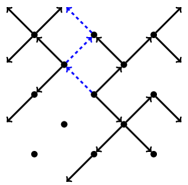
Figure 9: This figure shows a $3$-path in an instance of the random directed graph $G_{\textrm{r}}$.

Proof.

Let $A$ be a four-qubit Pauli operator different than the identity, and let $W$ be a four-qubit random Clifford unitary. Let us consider the random four-qubit Pauli operator $WAW^{\dagger}=\lambda B=\lambda B_{1}\otimes B_{2}\otimes B_{3}\otimes B_{4}$ and ignore the phase $\lambda$. Lemma 3 from [14] tells us that $B$ is uniformly distributed over the $4^{4}-1$ combinations of $B_{1},B_{2},B_{3},B_{4}\in\{\mathbbm{1},\sigma_{x},\sigma_{y},\sigma_{z}\}$ different than $B_{1}=B_{2}=B_{3}=B_{4}=\mathbbm{1}$. The factor $3^{x_{i}}$ follows from the fact that the value $x_{i}=0$ stands for the one case $B_{i}=\mathbbm{1}$, while the value $x_{i}=1$ stands for the three cases $B_{i}\in\{\sigma_{x},\sigma_{y},\sigma_{z}\}$. This proves formulas (19, 20, 21). ∎

Definition 6.

The random directed graph $G_{\textrm{r}}$ can be sampled by starting from $G$ and, at each vertex, remove the outwards arrows according to the probability distributions (19, 20, 21).

Definition 7.

An $l$-path in $G_{\textrm{r}}$ is a sequence of $l$ consecutive arrows starting at the central vertex and following the directions of the arrows (see Fig. 9).

In the lemma below we show that in order to upper-bound the probability that $G_{\textrm{r}}$ has no $l$-path, it is enough to analyse its lower quadrant, as represented in Fig. 10.

Definition 8.

The directed graph $G^{\triangle}$ is the lower quadrant of $G$, and the random directed graph $G^{\triangle}_{\textrm{r}}$ is the lower quadrant of $G_{\textrm{r}}$ (see Fig. 10).

Lemma 9.

The probability that $G_{\textrm{r}}$ has no $l$-path is upper-bounded by the probability that $G_{\textrm{r}}^{\triangle}$ has no $l$-path, that is

$${\rm prob}\{G_{\textrm{r}}\text{ has no }l\text{-path}\}\leq{\rm prob}\{G_{\textrm{r}}^{\triangle}\text{ has no }l\text{-path}\}\ .$$ (22)

Proof.

By definition, if $G_{\textrm{r}}^{\triangle}$ has an $l$-path then $G_{\textrm{r}}$ has an $l$-path too; therefore if $G_{\textrm{r}}$ has no $l$-path then $G_{\textrm{r}}^{\triangle}$ has no $l$-path. Using this, the bound follows. ∎

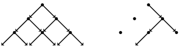
Figure 10: In the left we have the graph $G^{\triangle}$, and in the right we have an instance of the random directed graph $G^{\triangle}_{\textrm{ir}}$, both at time $t=3/2$.

III.3 Random graph with statistically-independent arrows

In order to simplify the analysis, we define a new graph where the probability for the presence of each arrow is independent of the presence of other arrows. The next lemma shows that it is sufficient to analyze this new graph.

Definition 10.

The random directed graph $G_{\textrm{ir}}^{\triangle}$ is sampled by taking $G^{\triangle}$ and independently removing each arrow with probability

$$q:={\rm prob}\{x=0\}=\frac{1}{2}-\frac{1}{2}\sqrt{\frac{21}{85}}\gtrapprox 0.25\ .$$ (23)

The subscript in $G_{\textrm{ir}}^{\triangle}$ stands “independent random arrows”. The meaning of the value of $q$ given above will become clear in the proof of lemma 11. As mentioned above we have the following.

Lemma 11.

The probability that $G_{\textrm{r}}^{\triangle}$ has no $l$-path is upper bounded by the probability that $G_{\textrm{ir}}^{\triangle}$ has no $l$-path:

$${\rm prob}\{G^{\triangle}_{\textrm{r}}\text{ has no }l\text{-path}\}\leq{\rm prob}\{G^{\triangle}_{\textrm{ir}}\text{ has no }l\text{-path}\}\ .$$ (24)

Proof.

First, note that the probability distribution of outwards arrows from different vertices are independent, and hence we focus only on a single vertex with two outwards arrows. Second, construct a matrix with the probability distribution $P(x_{1},x_{2})$ for the presence of outwards arrows (21) as

$$\begin{pmatrix}P(0,0)&P(0,1)\\ P(1,0)&P(1,1)\end{pmatrix}=\frac{1}{255}\begin{pmatrix}15&16\times 3\\ 16\times 3&16\times 9\end{pmatrix}\ .$$ (25)

Third, we increase ${\rm prob}\{x_{1}=x_{2}=0\}\to P(0,0)+\epsilon$ and decrease ${\rm prob}\{x_{1}=x_{2}=1\}\to P(1,1)-\epsilon$ until the distribution becomes of product form

$$\begin{pmatrix}P(0,0)+\epsilon&P(0,1)\\ P(1,0)&P(1,1)-\epsilon\end{pmatrix} =\begin{pmatrix}\frac{1}{17}+\epsilon&\frac{16}{85}\\ \frac{16}{85}&\frac{48}{85}-\epsilon\end{pmatrix}$$ (26)

$$=\begin{pmatrix}q^{2}&q(1-q)\\ q(1-q)&(1-q)^{2}\end{pmatrix}\ .$$ (27)

We want to find the minimum $\epsilon>0$ such that there is $q\in[0,1]$ satisfying the above equality. Clearly, this transformation cannot increase the likelihood of an $l$-path. The above matrix is of product form when its determinant is zero, in fact the second column of the last matrix in Eq. (26) is obtained from the first one multiplying by $\frac{1-q}{q}$.

$$\det\begin{pmatrix}\frac{1}{17}+\epsilon&\frac{16}{85}\\ \frac{16}{85}&\frac{48}{85}-\epsilon\end{pmatrix}=0\ .$$ (28)

This equation has smallest positive solution $\epsilon=\frac{1}{170}(43-\sqrt{1785})\approx 0.0044$, which implies

$$q=\frac{1}{17}+\epsilon+\frac{16}{85}=\frac{1}{2}-\frac{1}{2}\sqrt{\frac{21}{85}}\ .$$ (29)

This proves the statement of the lemma. ∎

III.4 Dual graph

Definition 12.

The graph $G_{\textrm{ir}}^{\triangle*}$ dual to $G_{\textrm{ir}}^{\triangle}$ has vertices located at the faces of $G_{\textrm{ir}}^{\triangle}$. The presence of a (non-directed) edge in $G_{\textrm{ir}}^{\triangle*}$ corresponds to the absence of the arrow it intersects in $G_{\textrm{ir}}^{\triangle}$. Therefore, the probability $q^{*}$ that an edge is absent in $G_{\textrm{ir}}^{\triangle*}$ is equal to the probability that an arrow is present in $G_{\textrm{ir}}^{\triangle}$, that is $q^{*}=1-q$, where $q$ is defined in (23). Figure 11 displays the graph dual to that of Fig. 10.

Definition 13.

A $d$-wall is a set of $d$ consecutive edges which connects the left side to the right side of $G_{\textrm{ir}}^{\triangle*}$.

Figure 11: Dual graph. On the left we have the dual graph $G^{\triangle*}$, and on the right we have the instance of the random graph $G_{\textrm{ir}}^{\triangle*}$ that is dual to the instance of $G_{\textrm{ir}}^{\triangle}$ shown in Fig. 10.

Lemma 14.

If $G_{\textrm{ir}}^{\triangle*}$ contains a $d$-wall then $G_{\textrm{ir}}^{\triangle}$ contains no $l$-path of length $l\geq d$.

Proof.

This follows from the fact that a $d$-wall must start in one of the first $d$ vertices of the left, and that $l$-paths always go downwards. ∎

Lemma 15.

The probability that $G_{\textrm{ir}}^{\triangle*}$ has a $d$-wall for some $d$ satisfies

$${\rm prob}\{\exists\,d:G_{\textrm{ir}}^{\triangle*}\text{ has }d\text{-wall}\}\leq 0.56\ .$$ (30)

Proof.

Let us start by upper-bounding the maximal number of $d$-walls $N_{d}$ that $G_{\textrm{ir}}^{\triangle*}$ can have. Consider a $d$-wall starting at a specific vertex position on the left side of $G_{\textrm{ir}}^{\triangle*}$. For the choice of the first edge in the path there is only one possibility, for the choice of each of the following $d-2$ edges there are at most three possibilities, and for the final edge there is a single choice (again). Hence, we can upper-bound the number of $d$-walls starting at a specific vertex on the left side by $3^{d-2}$. It is worth noting that this upper-bound includes many paths which do not connect the left and right sides, and hence, do not actually form a $d$-wall. The total number of vertices which can be the initial vertex (left side) of a $d$-wall is $d-1$. Hence, we have $N_{d}\leq(d-1)3^{d-2}$. In order to obtain a better bound we note that, when the starting vertex of a $d$-wall is either the $1^{\text{st}}$ or $(d-1)^{\text{th}}$ from the top, then there is only one possible choice of $d$-wall. Therefore, we obtain

$$N_{d}\leq(d-3)3^{d-2}+2\ .$$ (31)

Direct counting gives the exact number of $d$-walls for small values of $d$, which is displayed in the following table.

$$d$$ 2 3 4 5 6

1 2 3 6 18

(32)

Next, the probability that $G_{\textrm{ir}}^{\triangle*}$ contains a particular $d$-wall in $G^{\triangle*}$ is $(1-q^{*})^{d}=q^{d}$. Therefore, the probability that $G_{\textrm{ir}}^{\triangle*}$ has at least one $d$-wall satisfies

$${\rm prob}\{G_{\textrm{ir}}^{\triangle*}\text{ has }d\text{-wall}\}\leq N_{d}\,q^{d}\ .$$ (33)

Finally, the probability that $G_{\textrm{ir}}^{\triangle*}$ contains a $d$-wall of any length $d$ satisfies

$${\rm prob}\{ \exists\,d:G_{\textrm{ir}}^{\triangle*}\text{ has }d\text{-wall}\}$$

$$\leq\ \sum_{d=2}^{\infty}{\rm prob}\{G_{\textrm{ir}}^{\triangle*}\text{ has }d\text{-wall}\}\leq\ \sum_{d=2}^{\infty}N_{d}\,q^{d}$$ (34)

$$\leq\ \sum_{d=2}^{6}N_{d}\,q^{d}+\sum_{d=7}^{\infty}\left[(d-3)3^{d-2}+2\right]q^{d}$$ (35)

$$\approx 0.56\ ,$$ (36)

where we have use table (32) and bound (31). ∎

Combining lemmas 9, 11, 14 and 15 we can prove our main result.

Theorem 3. The probability that $G_{\textrm{r}}$ has an $l$-path of infinite length $l=\infty$ satisfies

$${\rm prob}\{G_{\textrm{r}}\text{ has }\infty\text{-path}\}\geq 0.44\ .$$ (37)

To conclude this section, let us note that while this proof of theorem 4 establishes the absence of localization in the 2D Floquet Clifford circuits (1), the lower bound given in Eq. (37) is probably not tight for practical purposes. Specifically, in our simulations of 2D circuits of finite size $L<\infty$, we find nontrivial operator support on the light-cone boundary for virtually all times and all random circuit realizations, such as in the example depicted in Fig. 1 (b).

IV Comparing Clifford dynamics with quasi-free bosons and fermions

In this section we argue that Clifford dynamics shares features with quasi-free systems, along with certain similarities with chaotic systems. Therefore, in order to elucidate the full landscape of quantum many-body phenomena, it is important to understand the properties of Clifford systems.

IV.1 General dynamics

Similarly to quasi-free fermions, Clifford unitaries can be represented by symplectic matrices in a phase space of dimension exponentially smaller than the Hilbert space. This dimensional reduction allows for efficient simulation of the evolution of any local or Pauli operator with a classical computer [64]. The efficient simulability of Clifford circuits can also be understood with respect to the non-negativity of the associated Wigner function in phase space [91, 92]. In particular, this non-negativity of the Wigner function of stabilizer states is analogous to the non-negative Wigner function of the Gaussian states corresponding to models with quadratic Hamiltonian [93, 94]. Furthermore, we have seen in Sec. III that Clifford dynamics allows for a certain degree of analytical tractability, which is similar to other types of integrable models.

Unlike quasi-free systems, the Clifford phase space is a vector space over a finite field ($\mathds{Z}_{2}^{2N}$ is the phase space of $N$ qubits) hence evolution cannot be continuous in time. That is, we can have Floquet-type but not Hamiltonian-type dynamics. For the same reason, the evolution operator cannot be diagonalised into non-interacting “modes”. Related to this is the fact that some aspects of typical Clifford dynamics cannot be understood in term of free or weakly-interacting particles [see for instance the dynamics in Fig. 1 (a)].

Random Clifford unitaries resemble uniformly distributed (i.e. Haar) unitaries much more than random quasi-free unitaries do. This can be made quantitative by using the notion of unitary design [95]. On one hand, random quasi-free unitaries cannot even generate a 1-design, because their evolution operators commute with the number operator (bosons) or the parity operator (fermions). On the other hand, random Clifford unitaries generate a 3-design [66, 67], and almost a 4-design [96].

As discussed in Sec. II.4, the SFF of Clifford unitaries corresponds to that of quasi-free fermions with chaotic single-particle dynamics, as in the quadratic SYK model [89, 90].

IV.2 Translation-invariant local dynamics

In [97] the authors analyze a translation-invariant Clifford Floquet model in one spatial dimension. They prove that the system has no local or quasi-local integrals of motion. More specifically, any operator that commutes with the evolution operator acts on an extensive number of sites with couplings among them that do not decay with the distance. This is very different to what happens with quasi-free systems, which have an extensive number of local conservation laws (see [98, 99]).

Unlike quasi-free systems, the Clifford model analyzed in [97] enjoys a strong form of eigenstate thermalization. That is, all eigenstates are maximally entangled in the sense that the reduced density matrix of any connected region is equal to the maximally-mixed state (in the thermodynamic limit). In other words, none of the eigenstates satisfy an entanglement area law.

IV.3 Disordered local dynamics

The 1D analog of our model (analyzed in detail in [14]) displays a strong form of localization produced by the emergence of left and right-blocking walls at random locations [see Fig. 1 (a)]. Until now, this strong form of localization, reminiscent of Anderson localization, has only been found in systems of free or weakly-interacting particles. In strongly-interacting systems the localization is in some sense weaker (many-body localization), since the width of the light-cones grows as the logarithm of time. Clifford dynamics appears to be some form of hybrid as it cannot be understood entirely in terms of free or weakly-interacting particles, but yet displays Anderson-type localization in 1D. Remarkably, however, the similarity in their localization properties does not carry over to 2D. More specifically, while we have shown in this paper that localization is absent in 2D random Floquet Clifford circuits, quasi-free systems, such as non-interacting fermions, are well-known to localize in 2D lattices even in the presence of arbitrarily weak disorder [100].

V Conclusions

We have introduced a Floquet model comprised of random Clifford gates and proved as a main result that it does not localize in two spatial dimensions, despite having strong disorder. More precisely, we have proven the existence of operators that grow ballistically, and we have seen numerically that this holds for almost all operators. This result is notable because, as discussed in Sec. IV, this model shares certain features of other integrable models, and two-dimensional integrable systems with strong disorder are usually expected to localize, e.g., non-interacting lattice fermions in a random potential as originally considered in the case of Anderson localization. We have substantiated our analytical findings by numerically demonstrating the absence (presence) of localization in 2D (1D) Floquet Clifford circuits. Furthermore, we studied the spectral form factor of the Floquet unitary, which is a key quantity in the context of quantum chaos. To the best of our knowledge, our work is the first to study the SFF in 2D Clifford circuits, complementing the analysis of Ref. [84], which has focused on 1D. We have unveiled that the SFF behaves drastically different in 2D. In particular, we observe a clean exponential ramp persisting up to a time that scales linearly with system size, which we interpret as a signature of ergodic dynamics in phase space.

It is worth noting that, since the definition of light-speed growth only concerns the boundary of the light-cone, our results also applies to the time-dependent (non-Floquet) version of the model, were new gates are randomly generated at each time step. For the same reason our results for the two-dimensional model extend to time-periodic circuits with time-period larger than two. The difference between models with period equal to two and models with a larger period or time-dependent models could manifest itself in the interior of the light cone. While the time-dependent model has completely ergodic dynamics, Fig. 5 (c) suggests that our time-periodic model is not far from it. While with our analytical methods we cannot address the interior of the light-cone, it might be interesting to extend our numerical analysis to probe whether the bulk of the light cone is indeed featureless or whether the Floquet circuit induces some structure on the Pauli strings that are sampled during the dynamics. Such potential differences compared with fully ergodic dynamics may for instance reflect themselves in the behavior of higher-order and non-local correlation functions that go beyond the local probe considered in Fig. 5.

In future work we would like to study the case where instead of sampling gates from the Clifford group we sample from the full unitary group SU(4). In the case of time-dependent circuits this has been well studied in references such as [3, 6, 101]. Whereas the case of time-periodic quantum circuits in one spatial dimension has been studied in references such as [49, 50, 51]. In this context, one promising approach to interpolate between Clifford dynamics and more generic Haar-random circuits is to consider circuits composed mainly of Clifford elements interspersed with a (low) density of non-Clifford gates, the latter acting as a seed of chaos which may enhance the ergodic aspects of the dynamics further [102, 103], despite loosing classical simulability [104]. Such a procedure may also help to better understand the apparent differences as well as similarities of Clifford dynamics and other notions of integrability [89, 90], a detailed exploration of which we believe to be an important direction of future work.

The localization proven for dynamics of a period-two, one-dimensional QCA of Cliffords in [14] and corroborated numerically in Fig. 5, as seen above, is known to disappear in the limit of a time-dependent circuit, as it also follows from [14]. Numerical investigations performed in [105] show that the one-dimensional circuit with period equal to four still localizes with the appearance of hard-walls that nevertheless are characterised by a larger localization length than the period-two case.

Finally, we would like to comment on the connections between our methods and directed percolation theory [106, 107]. Both cases analyze the presence of infinitely long paths which start at the origin in random directed graphs. But in our case, and in that of general cellular automata, the arrows that emerge from the same vertex are not statistically independent, see Lemma 5, while in the standard theory of directed percolation they are.

In conclusion, our work provides a new perspective on the possibility of using Clifford circuits to simulate certain novel nonequilibrium quantum phenomena. We expect that our work will inform future studies that aim to use Clifford circuits as starting points to understand more generic quantum dynamics.

The rigorous understanding of localization and chaos in this solvable limit provides a basis for toy models to simulate non-equilibrium states in kinetically constrained models. The classical simulability of Clifford circuits can play a constructive role for benchmarking the performance of noisy intermediate-scale quantum computers for quantum simulation and distinguishing between classical and quantum effects in them.

Acknowledgments

Tom Farshi acknowledges financial support by the Engineering and Physical Sciences Research Council (grant number EP/L015242/1 and EP/S005021/1) and is grateful to the Heilbronn Institute for Mathematical Research for support. Lluis Masanes and Daniele Toniolo acknowledge financial support by the UK’s Engineering and Physical Sciences Research Council (grant number EP/R012393/1). Daniele Toniolo also acknowledges support from UKRI grant EP/R029075/1. Jonas Richter and Arijeet Pal acknowledge funding by the European Research Council (ERC) under the European Union’s Horizon 2020 research and innovation programme (Grant agreement No. 853368). Jonas Richter also received funding from the European Union’s Horizon Europe programme under the Marie Skłodowska-Curie grant agreement No. 101060162.

Appendix

Appendix A Localization length in the 1D model

We present here a result that builds upon, and improves, theorem 25 of [14]. Let us first informally restate this theorem: The periodic dynamics of a one-dimensional QCA of two-qubits gates of uniformly sampled Clifford unitaries, represented as the inbox of Fig. 1, and Fig. 1 of [14], is such that the probability of appearance of a right (or left) blocking wall is at least $0.12$. If we consider only walls with penetration length equal to $1$, meaning that if for example a right-blocking wall is placed at $x=0$ then the support of an operator hitting that wall is allowed to flow only till $x=1$, then the probability of appearance of a wall is exactly equal to $0.12$. The proof of this statement rests on the use of the phase-space formalism for Clifford unitaries. The following corollary gives an upper bound on the average spread of the support of an operator initially non identity only at one point. This spread is the localization length $\mu$ that has been given in definition 1.

Corollary 16.

The periodic dynamics of a one-dimensional QCA of two-qubits gates of uniformly sampled Clifford unitaries is such that given an operator initially supported only on the site $x=0$, the probability that a wall blocking its dynamics appears at a distance $l$, and no other wall appears at $\{0,\dots,l-1\}$, is $ce^{-\frac{l}{\mu}}$, with $c\approx 0.07$ and $\mu$ upper bounded by $13.2$.

Proof.

Let us assume for simplicity that we consider a wall blocking propagation towards the right. According to the phase space formalism, as detailed in reference [14], see in particular section II E and section VII of [14], the absence of walls at neighboring positions, for example $x=0$ and $x=1$, are correlated events. In fact they satisfy the conditions: $C_{1}C_{0}\neq 0$ and$\setminus$or $C_{1}D_{0}A_{1}C_{0}\neq 0$ for the absence of a wall at $x=0$, and $C_{2}C_{1}\neq 0$ and$\setminus$or $C_{2}D_{1}A_{2}C_{1}\neq 0$ for the absence of a wall at $x=1$. Denoting $W_{l}$ the presence of a wall at $x=l$, and $\overline{W}_{l}$ the absence of a wall at $x=l$, we see that $\textrm{Prob}(\overline{W}_{1}\wedge\overline{W}_{0})=\textrm{Prob}(\overline{W}_{1}|\overline{W}_{0})\textrm{Prob}(\overline{W}_{0})$. This leads to a Markov chain, in fact the absence of a wall at $x=2$ involves the matrix blocks $\{C_{3},D_{2},A_{3},C_{2}\}$, we see that none of them appears in the condition defining $\overline{W}_{0}$. This means that the probability of having a wall at $x=l$ and no other wall at $\{0,\dots,l-1\}$ is given by:

$$\textrm{Prob}\left(W_{l}\wedge\overline{W}_{l-1}\wedge\dots\wedge\overline{W}_{0}\right)=$$

$$=\textrm{Prob}\left(W_{l}|\overline{W}_{l-1}\right)\textrm{Prob}\left(\overline{W}_{1}|\overline{W}_{0}\right)^{l-1}\textrm{Prob}\left(\overline{W}_{0}\right)$$

$$=\left(1-\textrm{Prob}\left(\overline{W}_{l}|\overline{W}_{l-1}\right)\right)\textrm{Prob}\left(\overline{W}_{1}|\overline{W}_{0}\right)^{l-1}\textrm{Prob}\left(\overline{W}_{0}\right)$$

$$=\left(1-\textrm{Prob}\left(\overline{W}_{1}|\overline{W}_{0}\right)\right)\textrm{Prob}\left(\overline{W}_{1}|\overline{W}_{0}\right)^{l-1}\textrm{Prob}\left(\overline{W}_{0}\right)$$

$$=\frac{\left(1-\textrm{Prob}\left(\overline{W}_{1}|\overline{W}_{0}\right)\right)\textrm{Prob}\left(\overline{W}_{0}\right)}{\textrm{Prob}\left(\overline{W}_{1}|\overline{W}_{0}\right)}\textrm{Prob}\left(\overline{W}_{1}|\overline{W}_{0}\right)^{l}$$ (38)

With the aid of a computer software we have exactly evaluated $\textrm{Prob}\left(\overline{W}_{1}|\overline{W}_{0}\right)=0.927$, and we recall from [14] that $\textrm{Prob}\left(\overline{W}_{0}\right)=0.88$. Then equation (38) implies that

$$\textrm{Prob}\left(W_{l}\wedge\overline{W}_{l-1}\wedge\dots\wedge\overline{W}_{0}\right)=ce^{-\frac{l}{\mu}}$$ (39)

with

$$c=\frac{\left(1-\textrm{Prob}\left(\overline{W}_{1}|\overline{W}_{0}\right)\right)\textrm{Prob}\left(\overline{W}_{0}\right)}{\textrm{Prob}\left(\overline{W}_{1}|\overline{W}_{0}\right)}\approx 0.07$$ (40)

$$\mu=-\frac{1}{\log\left(\textrm{Prob}\left(\overline{W}_{1}|\overline{W}_{0}\right)\right)}\approx 13.2$$ (41)

This proof takes into account walls with penetration length equal to 1, described by the Fig. 4 and 5 of [14]. Walls with larger penetration length are also allowed by the dynamics, taking them into account would lead to a shorter localization length, as confirmed by the numerics that leads to Fig. 5, therefore the value $\mu\approx 13.2$ is an upper bound. ∎

We comment about normalization of probability as a check that corollary 16 is consistent. In the limit of an infinite system the probability of having no wall at all is vanishing. This follows from the proof of corollary 16 where instead of evaluating $\textrm{Prob}\left(W_{l}\wedge\overline{W}_{l-1}\wedge\dots\wedge\overline{W}_{0}\right)$ we consider $\textrm{Prob}\left(\overline{W}_{l}\wedge\overline{W}_{l-1}\wedge\dots\wedge\overline{W}_{0}\right)$. This means that the probability of having at least one wall equals 1. The probability of having at least one wall is the sum of the probability of having a wall in $x=0$ and whatever else, plus the probability of having no wall in $x=0$ and a wall in $x=1$ and whatever else, plus the probability of having no wall in $x=0$ and no wall in $x=1$ and a wall in $x=2$ and whatever else, and so on. This means that:

$$1=\textrm{Prob}\left(W_{0}\right)+\sum_{l=1}^{\infty}\textrm{Prob}\left(W_{l}\wedge\overline{W}_{l-1}\wedge\dots\wedge\overline{W}_{0}\right)$$ (42)

It possible to verify that equation (42) is implied by equations (39), (40) and (41). We then have the normalized probability distribution $P(l)$ for the appearance of a wall at $x=l$ and no prior wall:

$$P(l)=\left\{\begin{array}[]{ll}\textrm{Prob}\left(W_{0}\right)=0.12&\mbox{ with }l=0\\ ce^{-\frac{l}{\mu}}&\mbox{ with }l\geq 1\\ \end{array}\right.$$ (45)

This implies that the average position of a wall is given by

$$\langle l\rangle=\sum_{l=1}^{\infty}lce^{-\frac{l}{\mu}}=\textrm{Prob}\left(\overline{W}_{0}\right)\mu+\mathcal{O}\left(1-\textrm{Prob}\left(\overline{W}_{1}|\overline{W}_{0}\right)\right)^{2}$$ (46)

This gives the relationship among the average position of a wall and the localization length $\mu$ in the limit of a large system.

References

- Polkovnikov et al. [2011] A. Polkovnikov, K. Sengupta, A. Silva, and M. Vengalattore, Rev Mod Phys 83, 863 (2011).
- Nahum et al. [2017] A. Nahum, J. Ruhman, S. Vijay, and J. Haah, Phys. Rev. X 7, 031016 (2017).
- Nahum et al. [2018] A. Nahum, S. Vijay, and J. Haah, Phys. Rev. X 8, 021014 (2018).
- von Keyserlingk et al. [2018] C. von Keyserlingk, T. Rakovszky, F. Pollmann, and S. Sondhi, Phys. Rev. X 8, 021013 (2018).
- Rakovszky et al. [2018] T. Rakovszky, F. Pollmann, and C. von Keyserlingk, Phys. Rev. X 8, 031058 (2018).
- Khemani et al. [2018] V. Khemani, A. Vishwanath, and D. A. Huse, Phys. Rev. X 8, 031057 (2018).
- Zhou and Nahum [2019] T. Zhou and A. Nahum, Phys Rev B 99, 174205 (2019).
- Brandão et al. [2021] F. G. Brandão, W. Chemissany, N. Hunter-Jones, R. Kueng, and J. Preskill, PRX Quantum 2, 030316 (2021).
- Potter and Vasseur [2021] A. C. Potter and R. Vasseur, (2021), arXiv:2111.08018 [quant-ph] .
- Moudgalya et al. [2021] S. Moudgalya, A. Prem, D. A. Huse, and A. Chan, Phys. Rev. Research 3, 023176 (2021).
- Gopalakrishnan and Zakirov [2018] S. Gopalakrishnan and B. Zakirov, Quantum Sci. Technol. 3, 044004 (2018).
- Bertini et al. [2019] B. Bertini, P. Kos, and T. Prosen, Phys Rev Lett 123, 210601 (2019).
- Claeys and Lamacraft [2021] P. W. Claeys and A. Lamacraft, Phys Rev Lett 126, 100603 (2021).
- Farshi et al. [2022] T. Farshi, D. Toniolo, C. E. González-Guillén, Á. M. Alhambra, and L. Masanes, Journal of Mathematical Physics 63, 032201 (2022).
- Richter et al. [2023] J. Richter, O. Lunt, and A. Pal, Phys. Rev. Res. 5, L012031 (2023).
- Arute et al. [2019] F. Arute et al., Nature 574, 505 (2019).
- Mi et al. [2021] X. Mi et al., Science 374, 1479 (2021).
- D’Alessio et al. [2016] L. D’Alessio, Y. Kafri, A. Polkovnikov, and M. Rigol, Adv Phys 65, 239 (2016).
- Gogolin and Eisert [2016] C. Gogolin and J. Eisert, Reports on Progress in Physics 79, 056001 (2016).
- Vidmar and Rigol [2016] L. Vidmar and M. Rigol, J. Stat. Mech: Theory Exp. 2016, 064007 (2016).
- Nandkishore and Huse [2015] R. Nandkishore and D. A. Huse, Annu Rev Conden Ma P 6, 15 (2015).
- Abanin et al. [2019] D. A. Abanin, E. Altman, I. Bloch, and M. Serbyn, Rev. Mod. Phys. 91, 021001 (2019).
- Stolz [2011] G. Stolz, Contemp Math 552, 71 (2011), 1104.2317 [math-ph] .
- Aizenman and Warzel [2015] M. Aizenman and S. Warzel, Random Operators: Disorder Effects on Quantum Spectra and Dynamics (AMS, 2015).
- Anderson [1958] P. W. Anderson, Phys Rev 109, 1492 (1958).
- Hamza et al. [2012] E. Hamza, R. Sims, and G. Stolz, Commun. Math. Phys. 315, 215 (2012).
- Abdul-Rahman et al. [2016] H. Abdul-Rahman, B. Nachtergaele, R. Sims, and G. Stolz, Lett Math Phys 106, 649–674 (2016).
- Deng et al. [2017] D.-L. Deng, X. Li, J. H. Pixley, Y.-L. Wu, and S. Das Sarma, Phys Rev B 95, 024202 (2017).
- nidari et al. [2008] M. nidari, T. Prosen, and P. Prelovek, Phys. Rev. B 77, 064426 (2008).
- Bardarson et al. [2012] J. H. Bardarson, F. Pollmann, and J. E. Moore, Phys. Rev. Lett. 109, 017202 (2012).
- Serbyn et al. [2013] M. Serbyn, Z. Papić, and D. A. Abanin, Phys. Rev. Lett. 110, 260601 (2013).
- Imbrie [2016] J. Z. Imbrie, J Stat Phys 163, 998 (2016).
- De Roeck and Huveneers [2017] W. De Roeck and F. Huveneers, Phys. Rev. B 95, 155129 (2017).
- untajs et al. [2020a] J. untajs, J. Bona, T. Prosen, and L. Vidmar, Physical Review B 102, 064207 (2020a).
- untajs et al. [2020b] J. untajs, J. Bona, T. Prosen, and L. Vidmar, Phys. Rev. E 102, 062144 (2020b).
- Sierant et al. [2020a] P. Sierant, M. Lewenstein, and J. Zakrzewski, Phys. Rev. Lett. 125, 156601 (2020a).
- Morningstar et al. [2022] A. Morningstar, L. Colmenarez, V. Khemani, D. J. Luitz, and D. A. Huse, Phys Rev B 105, 174205 (2022).
- De Roeck and Imbrie [2017] W. De Roeck and J. Z. Imbrie, Philosophical Transactions of the Royal Society A: Mathematical, Physical and Engineering Sciences 375, 20160422 (2017).
- Wahl et al. [2018] T. B. Wahl, A. Pal, and S. H. Simon, Nat Phys 15, 164 (2018).
- Sels and Polkovnikov [2021] D. Sels and A. Polkovnikov, Phys Rev E 104, 054105 (2021).
- Kiefer-Emmanouilidis et al. [2020] M. Kiefer-Emmanouilidis, R. Unanyan, M. Fleischhauer, and J. Sirker, Phys Rev Lett 124, 243601 (2020).
- Ghosh and nidari [2022] R. Ghosh and M. nidari, Phys. Rev. B 105, 144203 (2022).
- Richter and Pal [2022] J. Richter and A. Pal, Phys Rev B 105, l220405 (2022).
- D’Alessio and Rigol [2014] L. D’Alessio and M. Rigol, Physical Review X 4, 041048 (2014).
- Lazarides et al. [2014] A. Lazarides, A. Das, and R. Moessner, Physical Review E 90, 012110 (2014).
- Sünderhauf et al. [2018] C. Sünderhauf, D. Pérez-García, D. A. Huse, N. Schuch, and J. I. Cirac, Phys Rev B 98, 134204 (2018).
- Khemani et al. [2020] V. Khemani, M. Hermele, and R. Nandkishore, Physical Review B 101, 174204 (2020).
- Pai et al. [2019] S. Pai, M. Pretko, and R. M. Nandkishore, Physical Review X 9, 021003 (2019).
- Kos et al. [2018] P. Kos, M. Ljubotina, and T. Prosen, Phys. Rev. X 8, 021062 (2018).
- Bertini et al. [2018] B. Bertini, P. Kos, and T. Prosen, Phys Rev Lett 121, 264101 (2018).
- Bertini et al. [2020] B. Bertini, P. Kos, and T. Prosen, SciPost Phys. 8, 67 (2020).
- Chan et al. [2018a] A. Chan, A. De Luca, and J. T. Chalker, Phys Rev Lett 121, 060601 (2018a).
- Chan et al. [2018b] A. Chan, A. De Luca, and J. T. Chalker, Phys. Rev. X 8, 041019 (2018b).
- Bukov et al. [2015] M. Bukov, L. D’Alessio, and A. Polkovnikov, Adv Phys 64, 139 (2015).
- Khemani et al. [2016] V. Khemani, A. Lazarides, R. Moessner, and S. Sondhi, Phys Rev Lett 116, 250401 (2016).
- Else et al. [2016] D. V. Else, B. Bauer, and C. Nayak, Phys Rev Lett 117, 090402 (2016).
- Knill et al. [2008] E. Knill, D. Leibfried, R. Reichle, J. Britton, R. B. Blakestad, J. D. Jost, C. Langer, R. Ozeri, S. Seidelin, and D. J. Wineland, Phys Rev A 77, 012307 (2008).
- Magesan et al. [2011] E. Magesan, J. M. Gambetta, and J. Emerson, Phys Rev Lett 106, 180504 (2011).
- Onorati et al. [2019] E. Onorati, A. H. Werner, and J. Eisert, Phys. Rev. Lett. 123, 060501 (2019).
- Li et al. [2018] Y. Li, X. Chen, and M. P. A. Fisher, Phys Rev B 98, 205136 (2018).
- Li et al. [2021] Y. Li, R. Vasseur, M. P. A. Fisher, and A. W. W. Ludwig, Statistical mechanics model for clifford random tensor networks and monitored quantum circuits (2021), arXiv:2110.02988 [cond-mat.stat-mech] .
- Lunt et al. [2022] O. Lunt, J. Richter, and A. Pal, Quantum simulation using noisy unitary circuits and measurements, in Entanglement in Spin Chains: From Theory to Quantum Technology Applications, edited by A. Bayat, S. Bose, and H. Johannesson (Springer International Publishing, Cham, 2022) pp. 251–284, arXiv:2112.06682 [quant-ph] .
- Gottesman [1998] D. Gottesman, The Heisenberg Representation of Quantum Computers (1998), arXiv:quant-ph/9807006 [quant-ph] .
- Aaronson and Gottesman [2004] S. Aaronson and D. Gottesman, Phys Rev A 70, 052328 (2004).
- Harrow and Low [2009] A. W. Harrow and R. A. Low, Commun. Math. Phys. 291, 257 (2009).
- Webb [2016] Z. Webb, Quantum Information & Computation 16, 1379 (2016), arXiv:1510.02769 [quant-ph] .
- Zhu [2017] H. Zhu, Phys. Rev. A 96, 062336 (2017).
- Derrida and Stauffer [1986] B. Derrida and D. Stauffer, Europhysics Letters (EPL) 2, 739 (1986).
- Liu et al. [2021] S.-W. Liu, J. Willsher, T. Bilitewski, J.-J. Li, A. Smith, K. Christensen, R. Moessner, and J. Knolle, Physical Review B 103, 094109 (2021).
- Abrahams et al. [1979] E. Abrahams, P. W. Anderson, D. C. Licciardello, and T. V. Ramakrishnan, Phys Rev Lett 42, 673 (1979).
- Lee and Ramakrishnan [1985] P. A. Lee and T. V. Ramakrishnan, Rev. Mod. Phys. 57, 287 (1985).
- Evers and Mirlin [2008] F. Evers and A. D. Mirlin, Rev. Mod. Phys. 80, 1355 (2008).
- Farrelly [2020] T. Farrelly, Quantum 4, 368 (2020), arXiv:1904.13318 [quant-ph] .
- Gütschow et al. [2010] J. Gütschow, S. Uphoff, R. F. Werner, and Z. Zimborás, J Math Phys 51, 015203 (2010).
- Schlingemann et al. [2008] D.-M. Schlingemann, H. Vogts, and R. F. Werner, J Math Phys 49, 112104 (2008).
- Nielsen and Chuang [2010] M. A. Nielsen and I. L. Chuang, Quantum Computation and Quantum Information: 10th Anniversary Edition (Cambridge University Press, 2010).
- Chandran and Laumann [2015] A. Chandran and C. R. Laumann, Phys Rev B 92, 024301 (2015).
- Koenig and Smolin [2014] R. Koenig and J. A. Smolin, J Math Phys 55, 122202 (2014).
- Bravyi and Maslov [2021] S. Bravyi and D. Maslov, IEEE Trans. Inform. Theory 67, 4546 (2021).
- van den Berg [2020] E. van den Berg, (2020), arXiv:2008.06011 [quant-ph] .
- Hamma et al. [2005] A. Hamma, R. Ionicioiu, and P. Zanardi, Phys Rev A 71, 022315 (2005).
- Fattal et al. [2004] D. Fattal, T. S. Cubitt, Y. Yamamoto, S. Bravyi, and I. L. Chuang, (2004), arXiv:quant-ph/0406168 [quant-ph] .
- Haake [2010] F. Haake, Quantum Signatures of Chaos, 3rd ed. (Springer, 2010).
- Su [2020] S. Su, Chaos and Measurement-Induced Criticality on Stabiliser Circuits, Princeton University Senior Thesis (2020).
- Müller et al. [2004] S. Müller, S. Heusler, P. Braun, F. Haake, and A. Altland, Phys Rev Lett 93, 014103 (2004).
- [86] J. S. Cotler, G. Gur-Ari, M. Hanada, J. Polchinski, P. Saad, S. H. Shenker, D. Stanford, A. Streicher, and M. Tezuka, J High Energy Phys 10.1007/jhep05(2017)118.
- [87] H. Gharibyan, M. Hanada, S. H. Shenker, and M. Tezuka, J High Energy Phys 10.1007/jhep07(2018)124.
- Sierant et al. [2020b] P. Sierant, D. Delande, and J. Zakrzewski, Phys Rev Lett 124, 186601 (2020b).
- Winer et al. [2020] M. Winer, S.-K. Jian, and B. Swingle, Phys Rev Lett 125, 250602 (2020).
- Liao et al. [2020] Y. Liao, A. Vikram, and V. Galitski, Phys Rev Lett 125, 250601 (2020).
- Gross [2006] D. Gross, J Math Phys 47, 122107 (2006).
- Mari and Eisert [2012] A. Mari and J. Eisert, Phys Rev Lett 109, 230503 (2012).
- Hudson [1974] R. Hudson, Rep. Math. Phys. 6, 249 (1974).
- Weedbrook et al. [2012] C. Weedbrook, S. Pirandola, R. García-Patrón, N. J. Cerf, T. C. Ralph, J. H. Shapiro, and S. Lloyd, Rev Mod Phys 84, 621 (2012).
- Gross et al. [2007] D. Gross, K. Audenaert, and J. Eisert, J Math Phys 48, 052104 (2007).
- Zhu et al. [2016] H. Zhu, R. Kueng, M. Grassl, and D. Gross, (2016), arXiv:1609.08172 [quant-ph] .
- Zimborás et al. [2022] Z. Zimborás, T. Farrelly, S. Farkas, and L. Masanes, Quantum 6, 748 (2022).
- Bratteli and Robinson [2002] O. Bratteli and D. Robinson, Operator Algebras and Quantum Statistical Mechanics 2, 2nd ed. (Springer, 2002).
- Dierckx et al. [2008] B. Dierckx, M. Fannes, and M. Pogorzelska, J Math Phys 49, 032109 (2008).
- Lee and Fisher [1981] P. A. Lee and D. S. Fisher, Phys. Rev. Lett. 47, 882 (1981).
- Harrow and Mehraban [2023] A. W. Harrow and S. Mehraban, Commun. Math. Phys. 10.1007/s00220-023-04675-z (2023).
- Zhou et al. [2020] S. Zhou, Z.-C. Yang, A. Hamma, and C. Chamon, SciPost Phys. 9, 87 (2020).
- Haferkamp et al. [2023] J. Haferkamp, F. Montealegre-Mora, M. Heinrich, J. Eisert, D. Gross, and I. Roth, Commun. Math. Phys. 397, 995 (2023).
- Leone et al. [2021] L. Leone, S. F. E. Oliviero, Y. Zhou, and A. Hamma, Quantum 5, 453 (2021).
- Taylor [2022] J. Taylor, The Stability of Localisation in Random Time-Periodic Clifford Circuits, Master of Science dissertation, UCL, London (2022).
- Saberi [2015] A. A. Saberi, Phys. Rep. 578, 1 (2015).
- Durrett [1984] R. Durrett, Ann. Probab. 12, 999 (1984).