[1]
Hidden State Variability of Pretrained Language Models
Can Guide Computation Reduction for Transfer Learning
Abstract
While transferring a pretrained language model, common approaches conventionally attach their task-specific classifiers to the top layer and adapt all the pretrained layers. We investigate whether one could make a task-specific selection on which subset of the layers to adapt and where to place the classifier.The goal is to reduce the computation cost of transfer learning methods (e.g. fine-tuning or adapter-tuning) without sacrificing its performance.
We propose to select layers based on the variability of their hidden states given a task-specific corpus. We say a layer is already “well-specialized” in a task if the within-class variability of its hidden states is low relative to the between-class variability. Our variability metric is cheap to compute and doesn’t need any training or hyperparameter tuning. It is robust to data imbalance and data scarcity. Extensive experiments on the GLUE benchmark demonstrate that selecting layers based on our metric can yield significantly stronger performance than using the same number of top layers and often match the performance of fine-tuning or adapter-tuning the entire language model.
1 Introduction
Transfer learning from a pretrained language model (PLM) is now the de-facto paradigm in natural language processing (NLP). The conventional approaches of leveraging PLMs include fine-tuning all the parameters in the language model (LM) and some lightweight alternatives that can decrease the number of tuning parameters such as adapter-tuning (Houlsby et al., 2019; Hu et al., 2022; He et al., 2022) and prefix-tuning (Li and Liang, 2021). These methods have one thing in common: they all involve the entire PLM and attach a classifier to its top layer. However, PLMs were optimized via the language modeling objective and thus their top layers have been specialized in producing representations which facilitate optimizing that objective. Such mismatch between the pretraining and fine-tuning objectives poses the following questions:
-
① Given a pretrained language model and a downstream task, can we measure how “well-specialized” each layer has already been in that task, without any task-specific tuning?
-
② If the answer to ① is yes, can we use the layer-wise “task-specialty” as a guide in improving the computation efficiency of the transfer learning methods such as fine-tuning and adapter-tuning?
In this paper, we take a technically principled approach to investigate the research questions ① and ②. First, we define a metric in section 3.1 to measure the “task-specialty” of each layer in a given PLM. Our task-speciality score is inspired by the neural collapse (NC) phenomenon which has been widely observed in the computer vision community (Papyan et al., 2020): as training converges, the top-layer representations of the images with the same label form an extremely tight cluster. In our setting, we examine the variability of the representations of the linguistic sequences given by each layer of the PLM, and define our layer-wise task-specialty to be the within-class variability normalized by the between-class variability. Computing our metric does not require any training or hyperparameter tuning. Experiments on the GLUE benchmark demonstrate that it is highly correlated with layer-wise probing performance, thus giving a clear “yes” to the question ① above.
We propose several layer-selecting strategies in section 3.2 based on our proposed task-specialty metric. Our strategies are complementary to all the major paradigms of transfer learning (such as fine-tuning and adapter-tuning) and thus can take advantages of the state-of-the-art at the time: only the selected layers will be tuned (e.g., via fine-tuning or using adapters) such that the computation cost of the tuning methods can be further reduced. Experiments on the GLUE benchmark demonstrate that our proposed strategies are highly effective: under comparable computation budget, fine-tuning or adapter-tuning the layers selected by our strategies can achieve significantly higher performance than using the layers selected by the widely adopted baseline strategies; it can even often match the performance of fine-tuning or adapter-tuning the entire PLM which takes 500% more computation cost.
Through extensive ablation studies, we demonstrate the comparable advantages of our proposed task-specialty metric over potential alternatives (such as CCA and mutual information) as well as its robustness to data scarcity and data imbalance.
2 Technical Background
In this paper, we focus on classification tasks. Technically, each classification task has a corpus of training data where each is a sequence of linguistic tokens and each is a discrete class label. Such tasks include
-
•
Sentiment analysis. Each is a single sequence of words such as “This movie is fantastic” and is a sentiment label from . Thus, the sentiment analysis can be cast as a binary-class classification problem.
-
•
Natural language inference. Each is of the form “premise [SEP] hypothesis” such as “Fun for adults and children. [SEP] Fun for only children.” where “[SEP]” is a special separator token. The label indicates whether the premise entails the hypothesis. It is a three-class classification problem.
A PLM performs a classification task as follows:
-
1.
It reads each given sequence and embed it into a series of hidden state vectors
where denotes the hidden state of token given by layer and is a special classification (CLS) token.
-
2.
The top-layer hidden state of the CLS token is read by a neural network followed by a softmax layer, which gives the probability distribution over the target label :
(1) The net is also called “classification head”.
Transfer learning is to maximize the log probability of the ground-truth label —i.e., —by learning the parameters of the classification head as well as certain method-specific parameters:
- •
- •
- •
3 The Method
Our goal is to answer the research questions ① and ② introduced in section 1. That involves finding a layer-specific metric where each measures the task-specialty of layer . Suppose that we use to denote the task score that we can achieve by letting the classification head read the layer hidden state of the CLS token. If is highly (positively or negatively) correlated with , then the answer to question ① is yes. To answer question ② involves designing -based strategies that select a subset of layers to use in transfer learning approaches.
In this section, we introduce our task-specialty metric (section 3.1) along with a few strategies for selecting layers (section 3.2). In section 4, we will empirically demonstrate the effectiveness of our proposed metric and strategies.
3.1 Hidden State Variability Ratio
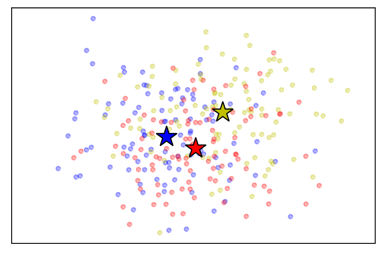
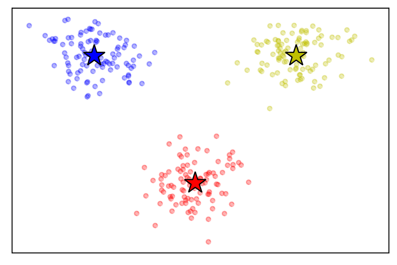
For a given task, we define our task-specialty metric based on the variability of the hidden state vectors that the PLM produces by embedding the training input sequences . We use hypothetical data to illustrate our intuition in Figure 1: after grouped based on the target labels , the variability of the hidden states within the same group (dots of same color) measures the difficulty of separating them, while the variability of the mean states (stars of different colors) quantifies how easy it is to tell the different groups apart.
Technically, for each layer , we first define the sequence-level hidden state for each input to be the average of the hidden states of all the (non-CLS) tokens . These sequence-level states correspond to the dots in Figure 1. Then we group all the based on the target labels : . The mean vector of each group is defined as and they correspond to the stars in Figure 1. The mean vector between classes is defined as . Then the within-group variability and between-group variability are defined using the sequence-level states and mean states:
Both and are a lot like covariance matrices since they measure the deviation from the mean vectors. Finally, we define our task-specialty metric to be the within-group variability scaled and rotated by the pseudo-inverse of between-class variability
| (3) |
The pseudo-inverse in equation 3 is why we use the average state as our sequence-level representation: averaging reduces the noise in the state vectors and thus leads to stable computation of .
We believe that the layers with small are likely to do better than those with large when transferred to the downstream task. Our belief stems from two key insights.
Remark-I: neural collapse.
Our proposed metric is mainly inspired by the neural collapse (NC) phenomenon: when training a deep neural model in classifying images, one can see that the top-layer representations of the images with the same label form an extremely tight cluster as training converges. Extensive theoretical and empirical studies show that a lower within-class variability can indicate a better generalization (Papyan et al., 2020; Hui et al., 2022; Galanti et al., 2022). Thus we examine the variability of the layer-wise representations of the linguistic sequences and hope that it can measure the task-specialty of each layer of the given PLM. Our metric is slightly different from the widely accepted neural collapse metric; please see section A.1 for a detailed discussion.
Remark-II: signal-to-noise ratio.
In multivariate statistics (Anderson, 1973), is able to measure the inverse signal-to-noise ratio for classification problems and thus a lower value indicates a lower chance of misclassification. Intuitively, the between-class variability is the signal which one can use to tell different clusters apart while the within-class variability is the noise that makes the clusters overlapped and thus the separation difficult; see Figure 1 for examples.
Remark-III: linear discriminant analysis.
A low implies that it is easy to correctly classify the data with linear discriminant analysis (LDA) (Hastie et al., 2009). Technically, LDA assumes that the data of each class is Gaussian-distributed and it classifies a new data point by checking how close it is to each mean vector scaled by the covariance matrix which is typically shared across classes. Though our metric does not make the Gaussian assumption, a low suggests that the class means are far from each other relative to the within-class variations , meaning that the decision boundary of LDA would tend to be sharp. Actually, our is an estimate to the Gaussian covariance matrix of LDA.
3.2 Layer-Selecting Strategies
Suppose that our metric can indeed measure the task-specialty of each layer. Then it is natural to investigate how the knowledge of layer-wise task-specialty can be leveraged to improve the transfer learning methods; that is what the question ② in section 1 is concerned with. Recall from section 2 that the major paradigms of transfer learning use all the layers of the given PLM by default. We propose to select a subset of the layers based on the their task-specialty which will benefit all the paradigms of transfer learning: they may be able to only use the selected layers yet still achieve strong performance. Only using the selected layers will result in significant reduction of computation cost:
-
•
In fine-tuning, only the parameters of the selected layers will be updated.
-
•
In adapter-tuning, adapters are only added to the selected layers but not all the layers.
-
•
In prefix-tuning, we “deep-perturb” fewer layers.
A smaller number of task-specific parameters means not only less training cost but also less storage cost and less inference cost.
Strategy-I: -down.
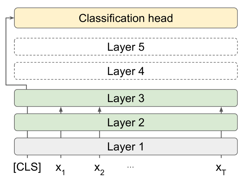
We use to denote the layer which achieves the best task-specialty: i.e., . Our first strategy is motivated by the following intuition: if layer has already been well-specialized in the given task, then it may suffice to just mildly tune it along with a few layers below it. Meanwhile, we may keep the classification head on the top layer or move it to the best-specialized layer : the former still utilizes the higher layers in training and inference; the latter does not and thus will result in even less computation and memory cost.
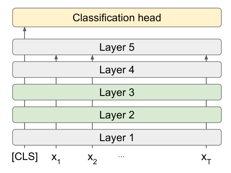
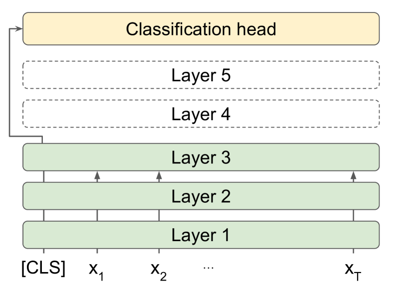
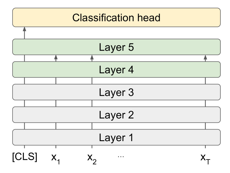
Technically, we use to denote the strategy of selecting the layers and connect the classification head to the layer . Then all the instances of our first strategy can be denoted as or with appropriately chosen . Figures 2(a), 2(b) and 2(c) illustrate a few specific instances of our -down strategy.
Strategy-II: -up.
Alternative to the -down strategy, our second strategy is to select the layers above the best-specialized layer and we call it -up strategy. Intuitively, if layer is already well-specialized in the given task, then what we need is perhaps just a powerful classification head. That is, we can regard the higher layers along with the original classification head as a new “deep” classification head and then tune it to better utilize the layer representations.
In principle, all the instances of our second strategy can be denoted as or since we may select the layers up through and move the classification head to layer . Figure 2(d) shows an instance of our -up strategy.
Note that our notation can apply to the conventional layer-selecting strategies as well. For example, denotes the naive option of tuning all the layers of the given PLM; denotes a baseline method of only selecting the top three layers.
4 Experiments
We evaluated the effectiveness of our task-specialty metric along with our layer-selecting strategies through extensive experiments on the six classification tasks of the GLUE benchmark (Wang et al., 2019). The tasks are: CoLA, MNLI, MRPC, QNLI, QQP, and SST-2.All of them are sequence-level classification tasks related to natural language understanding, thus being very different from how language models are pretrained.
We chose the widely accepted RoBERTa model (Liu et al., 2019b) to be our PLM and used the pretrained roberta-large instance (355M parameters) downloaded from HuggingFace (Wolf et al., 2020). Our experiments are mainly conducted with this model. We also experimented with DeBERTa (He et al., 2020) to investigate whether our methods generalize across models:111Bowman (2022) advocate that it is important to experiment with more than one pretrained models before drawing any general conclusions about “pretrained language models”. those results are in section C.2 and are similar to the RoBERTa results. Prior work (Mosbach et al., 2020a) found that fine-tuning RoBERTa on GLUE could be unstable, so we ran each of our experiments with five random seeds and reported the means and standard errors. Experiment details (e.g., hyperparameters) can be found in Appendix B.
Our code is implemented in PyTorch (Paszke et al., 2017) and heavily relies on HuggingFace. It will be released after the paper is published. Implementation details can be found in section B.2.
4.1 Answer to Question ①: Hidden State Variability Ratio Measures Task-Specialty
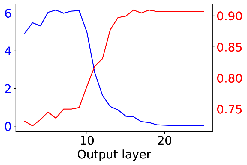
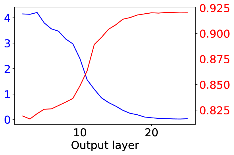
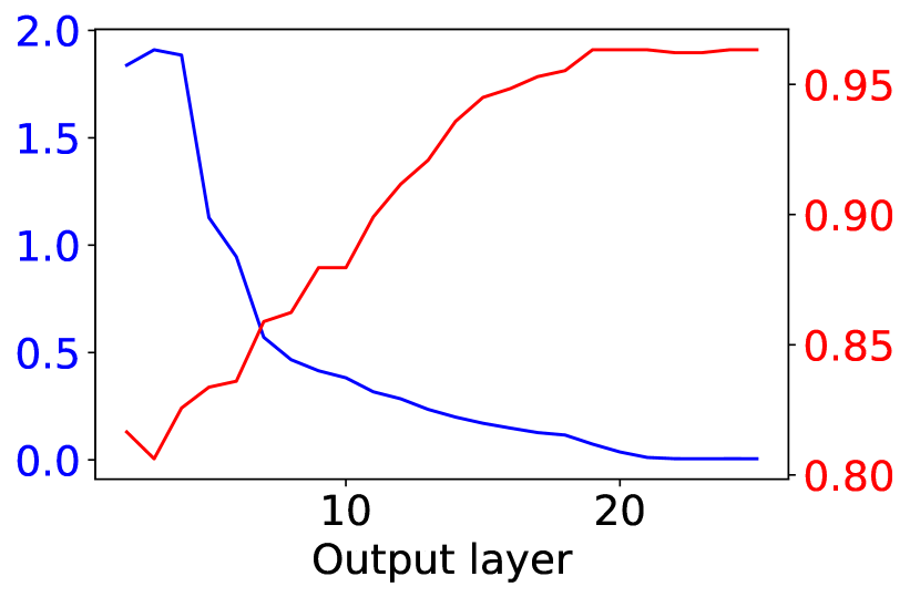
For each task, we computed the task-specialty (defined in section 3.1) for all the 24 layers. They are plotted as blue curves in Figure 3: as we can see, the middle layers () tend to have the lowest on most tasks.
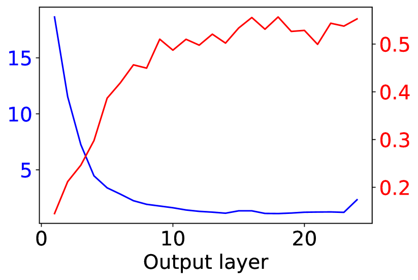
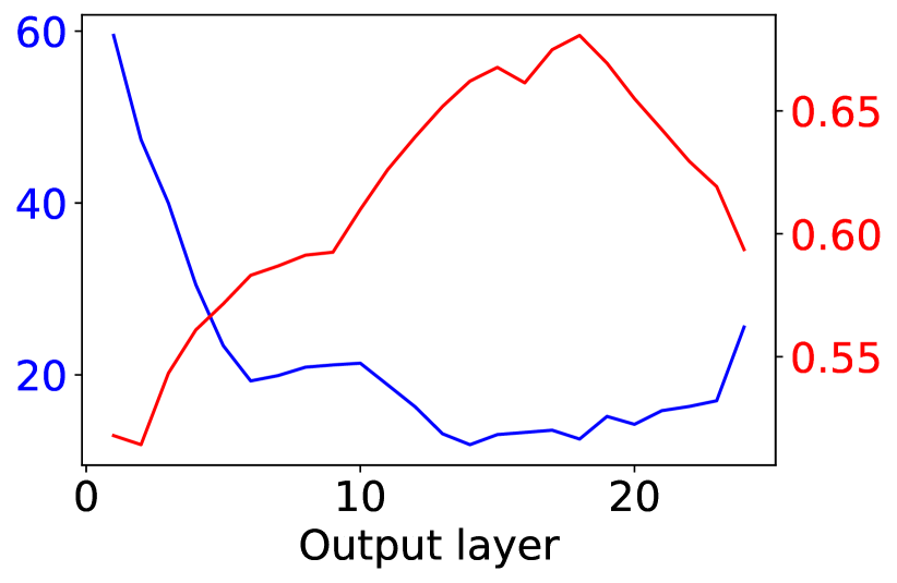
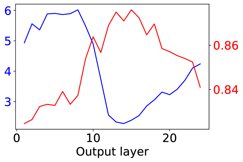
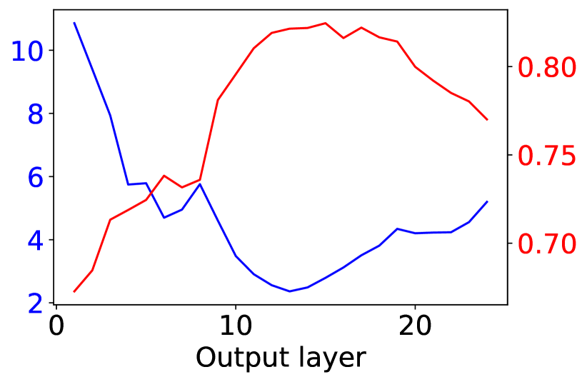
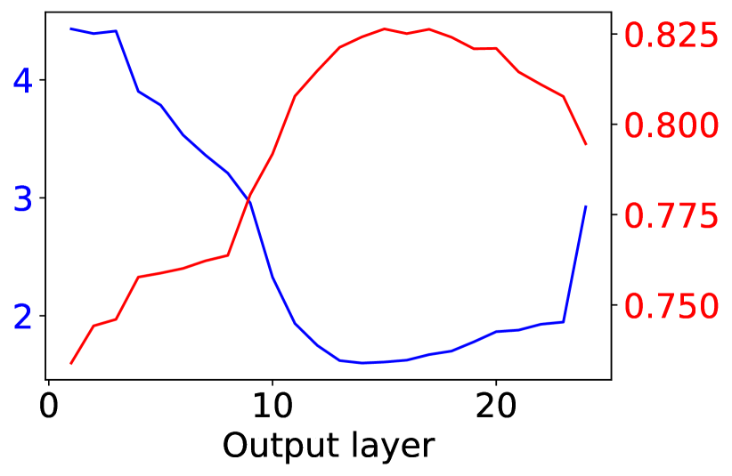
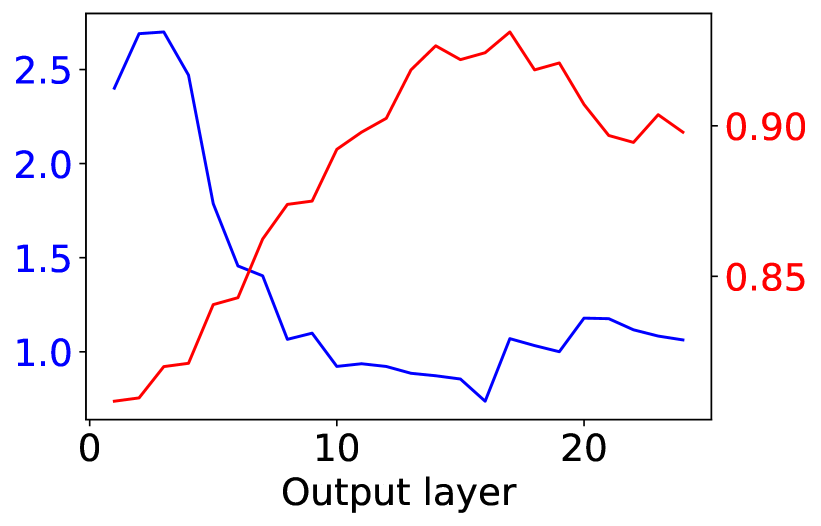
Then we probed the pretrained RoBERTa: for each layer , we trained a classification head (see section 2) that reads the hidden state and evaluated it on the held-out development set. The probing performance is plotted as red curves in Figure 3: as we can see, the middle layers () tend to achieve the highest scores.
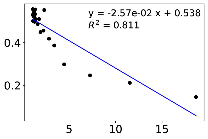
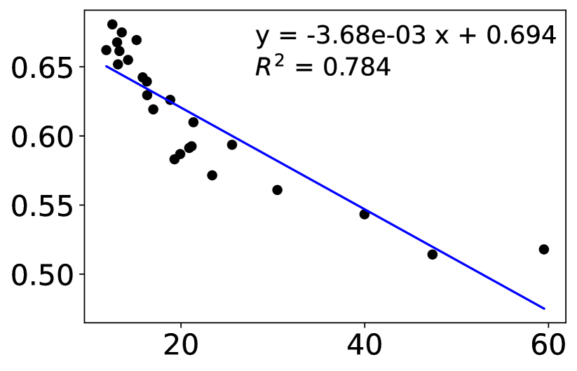
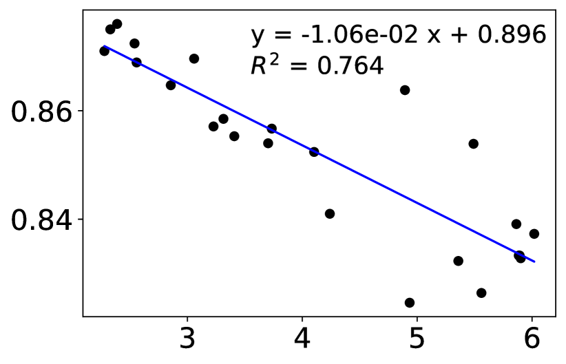
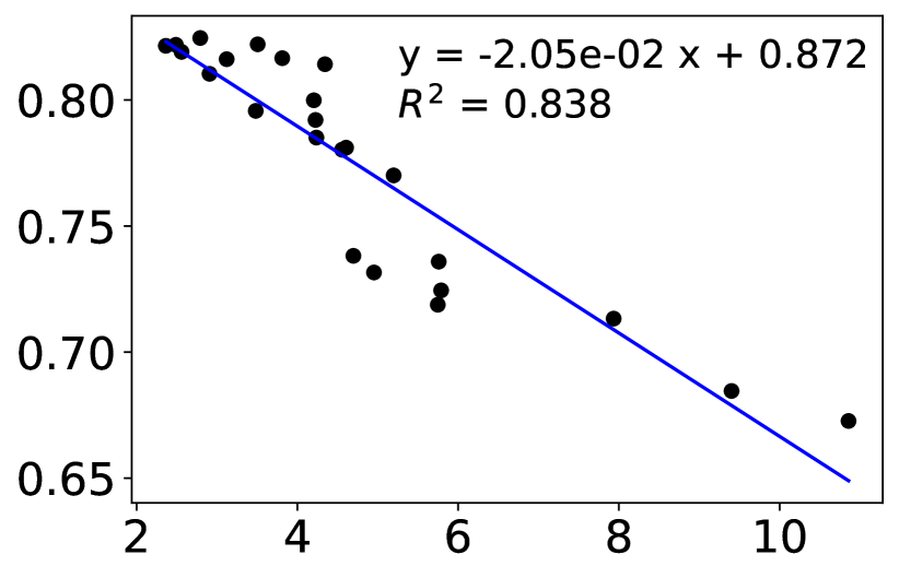
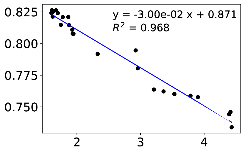
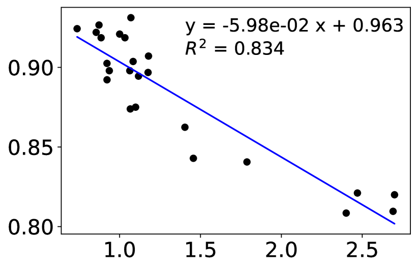
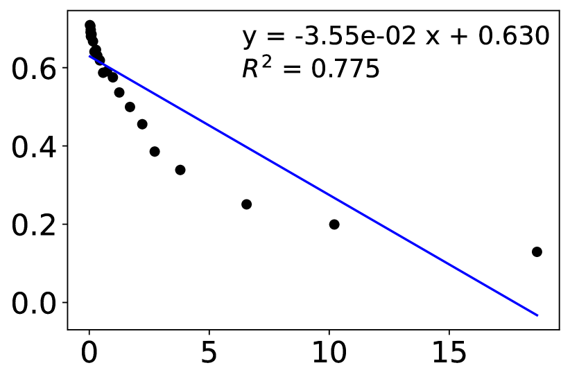
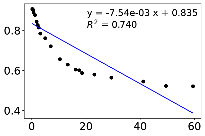
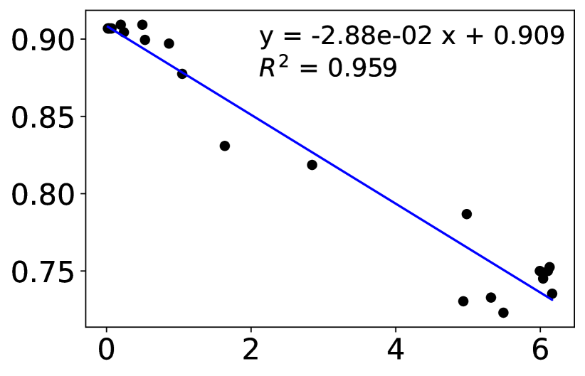
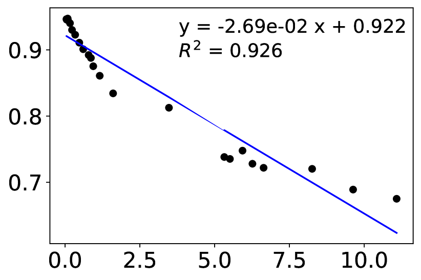
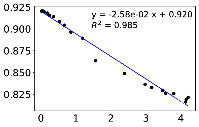
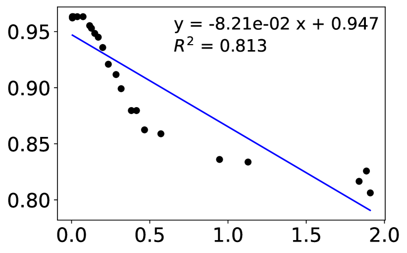
How much is the probing performance correlated with the task-specialty metric ? To answer that question, we regressed the probing performance on and found that they are highly correlated. All the slope coefficients are negative, meaning that a low predicts a high score. All the are high, meaning that a large fraction of the probing performance variation can be explained by the variation in the task-specialty score. Remarkably, on QQP. Detailed results (e.g., fitted lines) are in Figure 11 of section C.3.
This set of experiments answers our question ① (section 1): yes, we can measure the task-specialty of each layer of a given PLM on a given task and our metric doesn’t require task-specific tuning.
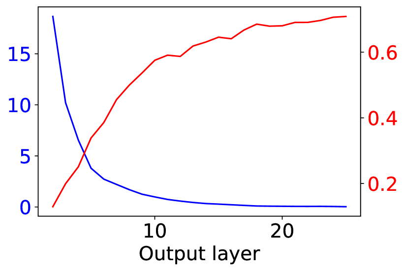
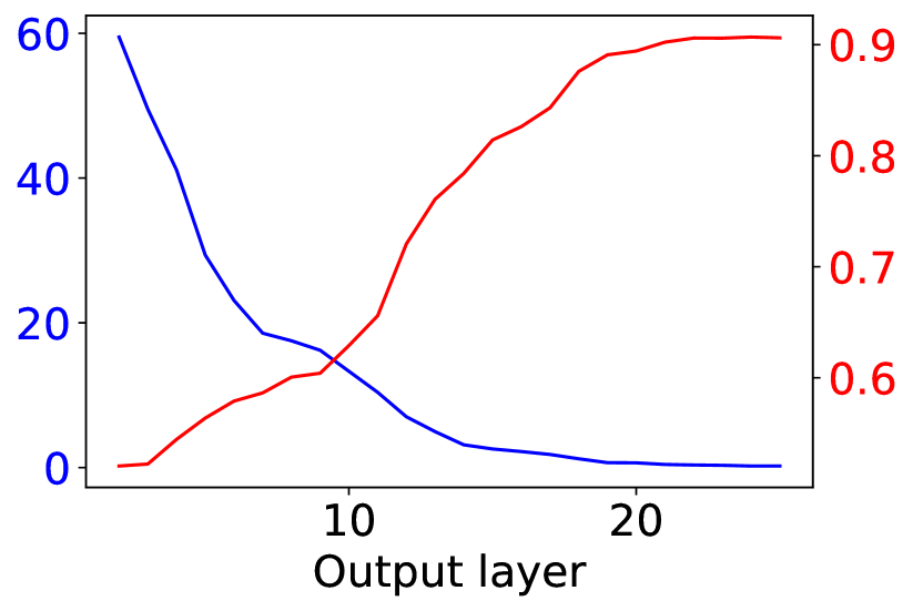
Furthermore, we fully fine-tuned a RoBERTa on each task and obtained the and probing performance of the fine-tuned models. The results are presented in Figures 12 and 13 of section B.4. After full fine-tuning, strong correlation between the probing performance and the task-specialty is still observed, but now higher layers are observed to have lower and stronger probing performance. That is because the parameters of higher layers have received stronger training signals back-propagated from the classification heads, which aim to specialize the full model on the tasks.
4.2 Answer to Question ②: Task-Specialty Helps Layer Selection
As discussed in section 3.2, our task-specialty-based layer-selecting strategies are supposed to help improve the computation efficiency of transfer learning and they are compatible with all the major paradigms of transfer learning. We evaluated our strategies by pairing them with the widely adopted fine-tuning and adapter-tuning methods. In this section, we show and discuss our empirical results.
Layer selection for fine-tuning.
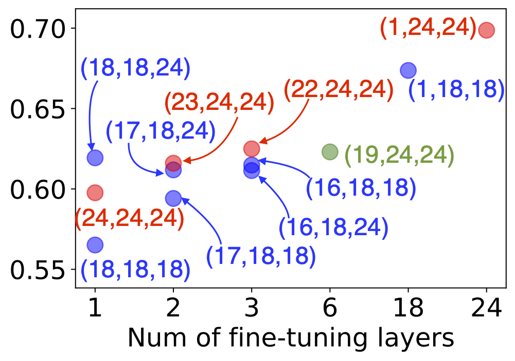
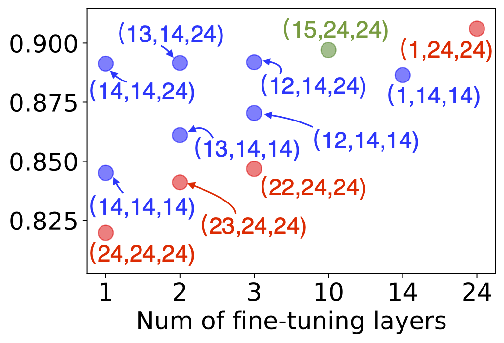
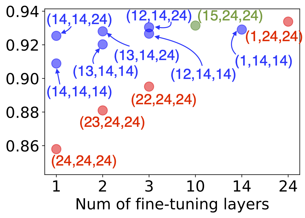
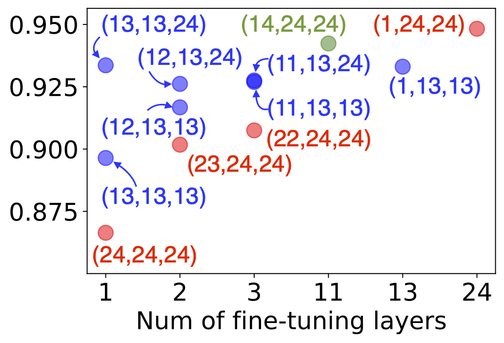
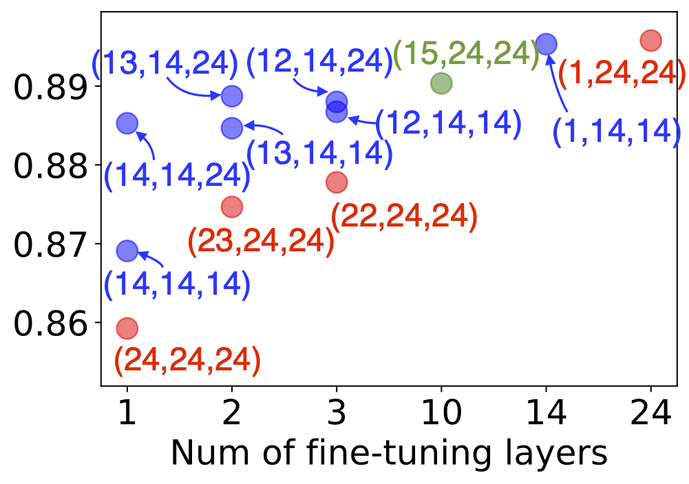
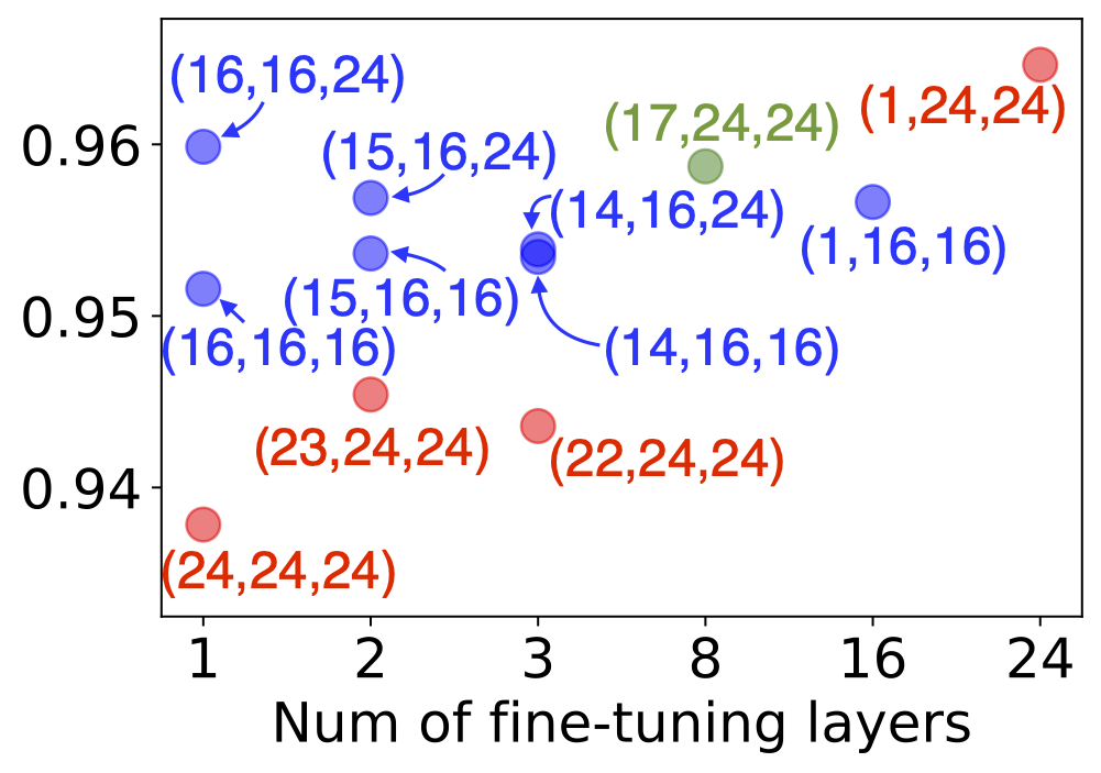
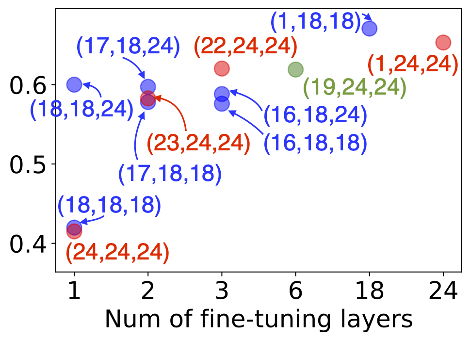
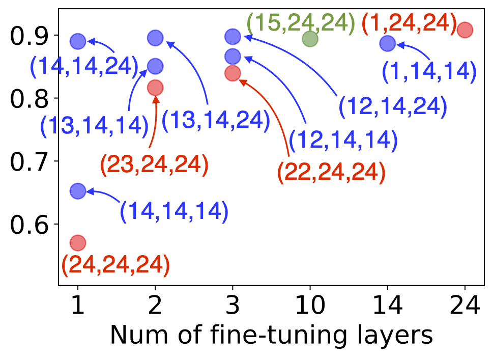
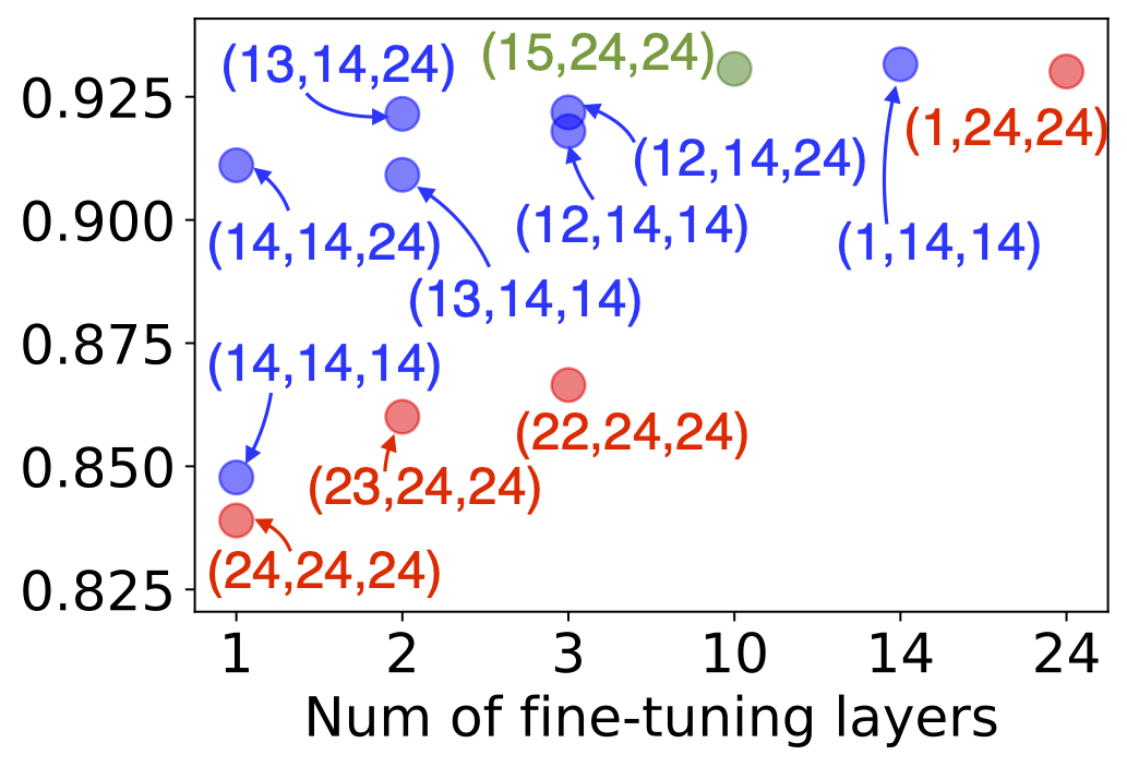
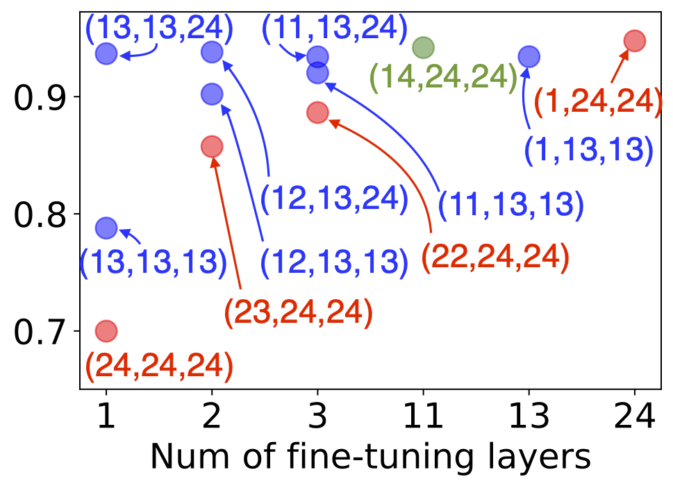
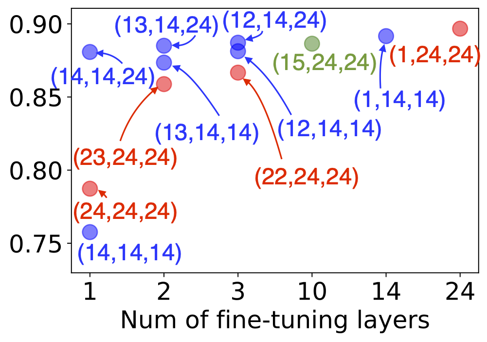
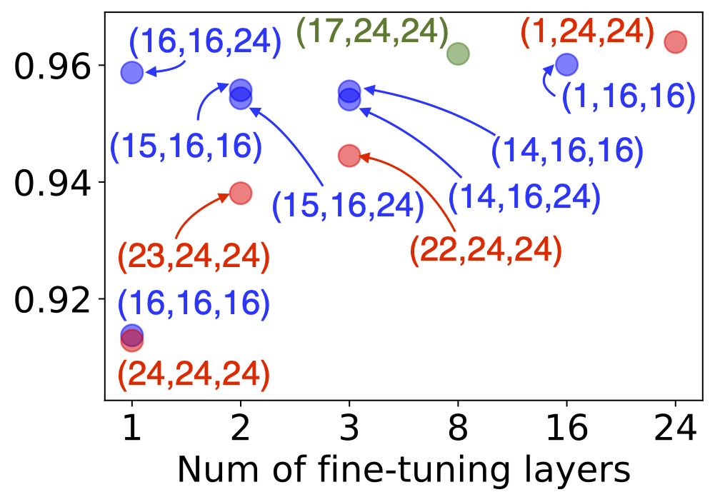
For each task, we experimented with our -down and -up strategies. The best-specialized layers are those with the lowest task-specialty . They are
| CoLA | MNLI | MRPC | QNLI | QQP | SST-2 | |
|---|---|---|---|---|---|---|
| 18 | 14 | 14 | 13 | 14 | 16 |
Our experiment results are shown in Figure 4. For the -down strategy, we experimented with where and . They are plotted as blue dots. For the -up strategy, we experimented with and they are shown as green dots. For a comparison, we also experimented with the conventionally adopted baseline strategies and with . They are red dots. The actual performance scores of the dots along with standard errors are in Table 6 of section C.1.
As shown in Figure 4, when we are constrained by a budget of tuning only layers, our strategies can almost always lead to significantly higher performances than the baseline strategies. Moreover, the strategies consistently outperform the strategies across all the tasks. It means that the higher layers are still very useful for performing well on the given task even if their parameters are not updated: they are perhaps able to help shape the training signals back-propagated through the tuned layers.
Furthermore, the performance of only tuning the selected layers is often close to that of full fine-tuning. Remarkably, on QQP, our strategy even matches the performance of full fine-tuning yet only uses the bottom 14 layers; that is, it reduces the computation and storage cost by more than 40%. Detailed discussion about wall-clock time saving can be found in section C.1.
Because most are in the middle of the PLM, we experimented another baseline of directly using the middle layer for the -layer RoBERTa-large. This baseline is only implemented on CoLA and SST-2 because of other tasks is already the same as or very close to . We found that tuning around layer always outperforms tuning around although the improvement is not large. Result details are in Table 8 of section C.1.
Layer selection for adapter-tuning.
For adapter-tuning, we implemented the earliest adapter architecture designed by Houlsby et al. (2019). We experimented with the same set of our strategies and baseline strategies as in the fine-tuning experiments. The results are plotted in Figure 5. Detailed numbers including standard errors are listed in Table 7 in section C.1.
Like for fine-tuning, in most cases, our strategies are significantly better than the baseline strategies under the budget of tuning only layers. The strategies also tend to outperform the strategies.
What’s impressive is that the performance of only adapter-tuning the selected layers is often comparable to that of full adapter-tuning. Surprisingly, on MNLI and QNLI, our and strategies match the full adapter-tuning but only need 12% and 8% of the trainable parameters as full adapter-tuning respectively.
We also implemented the middle layer baseline for adapter-tuning on CoLA and SST-2. The results are listed in Table 9 of section C.1. In most cases, outperforms with the same number of adapted layers.
Interestingly, Houlsby et al. (2019) also found that not every layer in the PLM is equally important for adapter-tuning. For example, they experimented with a 12-layer BERT model and found that ablating the layer-7 adapters will lead to a much larger performance drop than ablating those of the top three layers on the CoLA task.
4.3 Is Our Metric the Only Option?
In this section, we will discuss a few potential alternatives to our proposed task-specialty metric . The introduction of the alternatives will be brief and only focused on their definitions and intuitions; more details can be found in section C.7.
| Task | |||
|---|---|---|---|
| CoLA | -0.901 | 0.977 | -0.914 |
| MNLI | -0.885 | 0.977 | -0.493 |
| MRPC | -0.874 | 0.934 | -0.593 |
| QNLI | -0.915 | 0.988 | -0.514 |
| QQP | -0.984 | 0.989 | -0.723 |
| SST-2 | -0.913 | 0.986 | -0.798 |
Canonical correlation analysis.
A potential alternative to our proposed metric is the canonical correlation between the hidden states and the class labels . Canonical correlation analysis (CCA) involves learning a series of projection parameters such that each maximizes the correlation between and under certain constraints: is a one-hot vector with its th entry being one.
Numerical Rank.
Another potential alternative is the rank-based metric proposed by Zhou et al. (2022). It is also inspired by the neural collapse phenomenon. The intuition is: if the sequence-level representations of the same exhibit a low variability, then the matrix formed by the vectors in will have a low rank since its columns will be similar. The rank of can be estimated by where is the nuclear norm (i.e., the sum of singular values) and is the Frobenius norm. The rank-based metric is the average over : . The correlation between and the probing performance is presented in Table 1.
Analysis.
As we can see in Table 1, our variability-based metric and CCA score both exhibit a high correlation (above 0.85) with the probing performance. The correlation of CCA is moderately better than ours and it is higher than 0.9 on all the tasks. However, CCA optimization is dependent on the regularization terms (see section C.7) and thus requires cross-validation to choose the right set of hyperparameters. This makes it more involved to compute than the proposed variability metric. Technically, CCA requires a “training procedure” to fit a set of parameters ( and ) though the computation of that part is as light as calculating our metric. Both CCA and our metric are scale invariant. Overall, the rank-based metric has a lower correlation. That is because it only considers the within-group properties but ignores the between-group properties.
4.4 Ablation Studies and Analysis
Averaged state vs. CLS state.
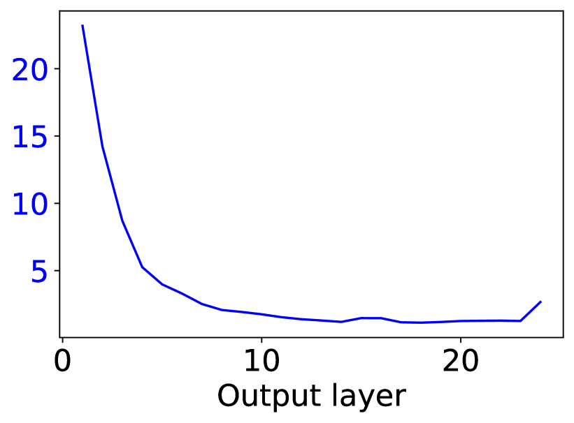
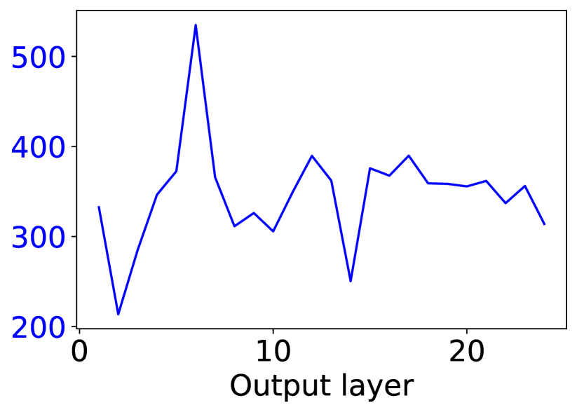
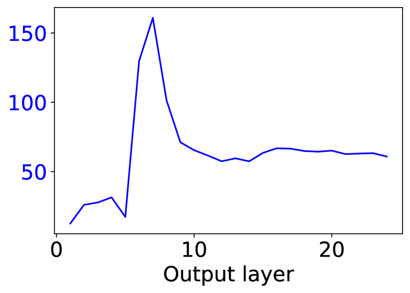
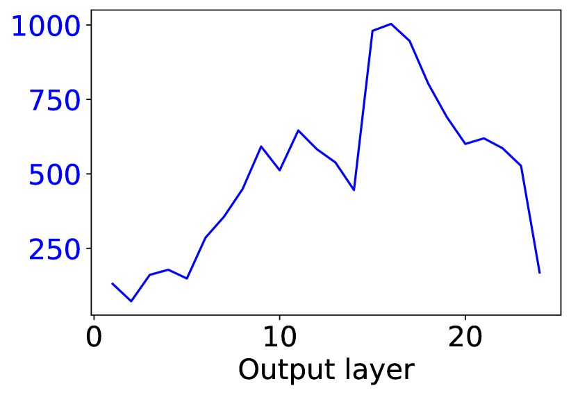
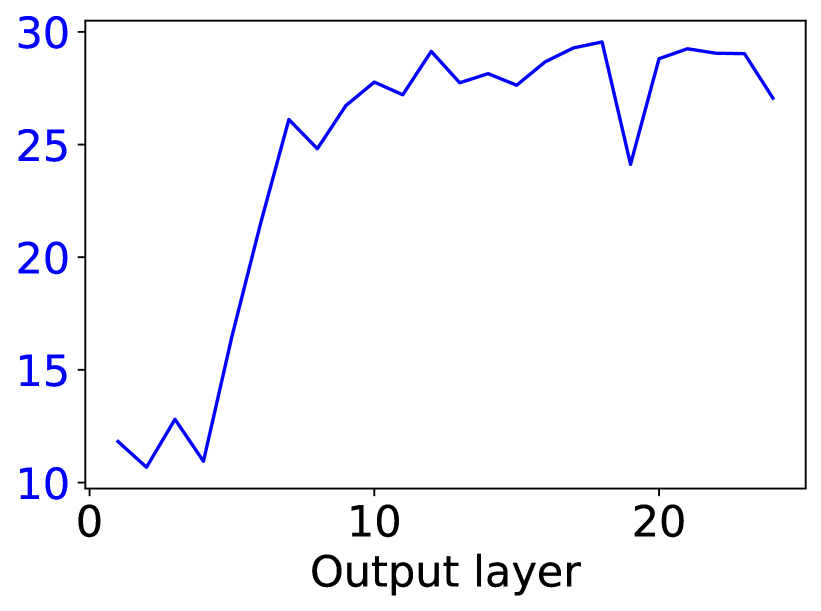
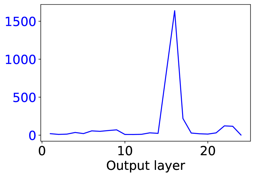
The that we have reported so far are all computed using the average hidden state of each as defined in section 3.1. We also experimented with the CLS token hidden states—i.e., —and found that the computation of became much less stable: e.g., on SST-2, the metrics of the pretrained RoBERTa are below 50 for most of the layers but can jump above 500 for a couple of layers. Intuitively, one would like to trust a curve that is at least locally smooth. Technically, local smoothness means a small local second-order derivative, which can be estimated by finite differences. Therefore, we measure the local smoothness of a curve by the following quantity
The results222We normalized the values before computing so that the and are more comparable across different choices of the sequence-level representation. Our normalization is: where and is the mean and standard deviation of the original . are presented in Table 2.
| Task | with averaged state | with CLS state |
|---|---|---|
| CoLA | 0.950 | 0.949 |
| MNLI | 1.347 | 88.162 |
| MRPC | 1.994 | 33.038 |
| QNLI | 3.256 | 13.566 |
| QQP | 1.640 | 7.629 |
| SST-2 | 3.604 | 58.040 |
As we can see, the computed using the CLS token states is dramatically larger than that of using the averaged states on all the tasks except CoLA. It means that using the averaged states will give us a more trustable curve.Thus, we used the average hidden states throughout our experiments; we made this choice before seeing any task performance.
The actual curves computed using the CLS states are presented in Figure 14 of section C.5.
Robustness to data imbalance.
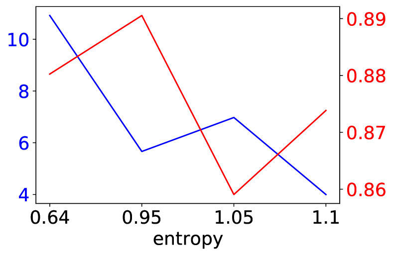
The datasets of GLUE tasks are almost perfectly balanced. So it remains a question whether our proposed task-specialty is still effective when the data is not imbalanced. To answer this question, we synthesized a series of data-imbalanced experiments on SST-2. In each experiment, we randomly sampled training examples with a portion from the negative class where . We did the same analysis on MNLI; see results in section C.6.
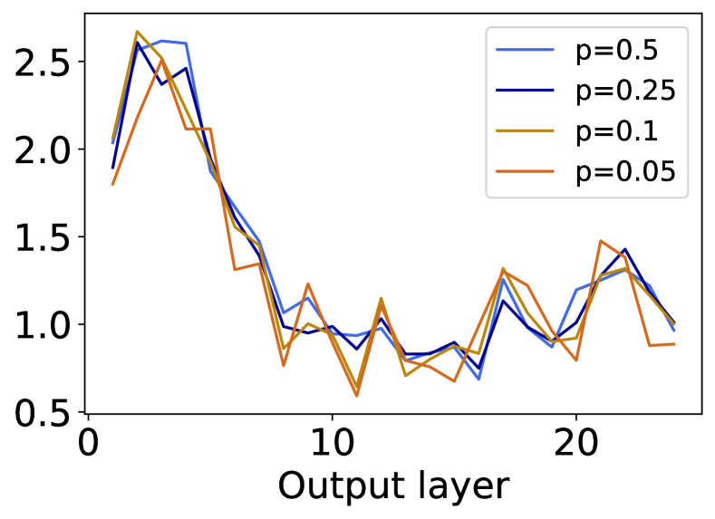
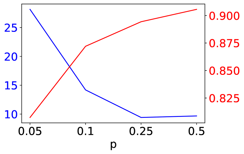
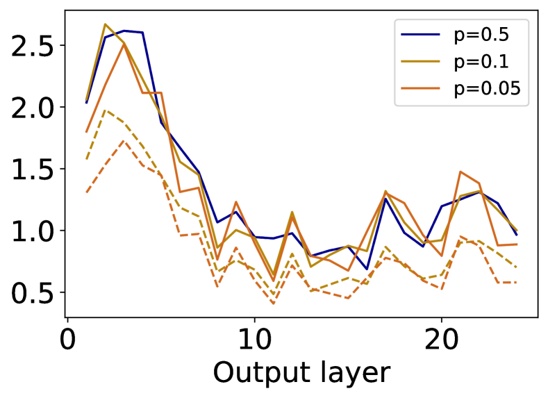
For each experiment, we plot the curve in Figure 6(a). We also computed the local smoothness score and the absolute value of the correlation (defined in section 4.3) and plot them in Figure 6(b). Interestingly, the in the case of is as low as that of , though it becomes much larger when the data is extremely imbalanced (e.g., ). Moreover, the is still above 0.85 even when . Those findings mean that our task-specialty metric is reasonably robust to data imbalance. More details are in section C.6.
Robustness to data scarcity.
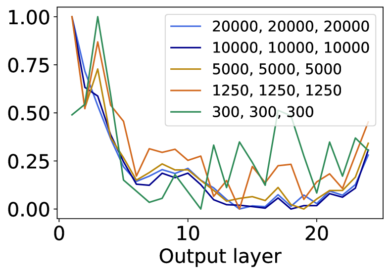
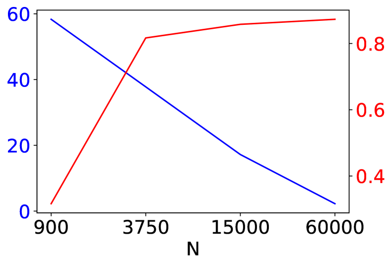
We also examined the robustness of our metric to data scarcity. On SST-2, we conducted a series of experiments with varying number of training samples: . For each experiment, we made the sampled dataset label-balanced. See the results on MNLI in section C.6.
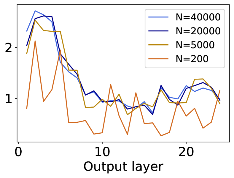
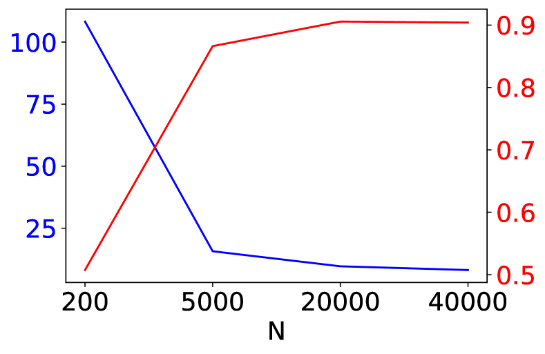
Like in the data-imbalanced experiments, we plot and and in Figure 7. As we can see, for , the curves almost perfectly overlap and the and only slightly change with . It means that the values are trustable as long as they are computed using thousands of examples. In the extremely data-scarce case of , the curve becomes not trustable: after all, it will be extremely difficult to estimate and with so few samples. However, even in the case of , the middle layers tend to have the lowest which agree with the data-adequate cases. More details are in section C.6.
5 Related Work
Analysis of PLMs.
Representations from PLMs have been widely studied using probing methods.333In this paper, we focus on the models that are pretrained only with the language modeling objective. Other pretraining objectives such as those of Sun et al. (2019); Wang et al. (2021); Raffel et al. (2020) are out of our current scope. There is evidence showing that pre-trained features from intermediate layers are more transferable (Tenney et al., 2019; Rogers et al., 2020). Additionally, Voita et al. (2019a) show that masked language modelling objective introduces an auto-encoder like structure in the PLM, meaning the behaviour of the top most layers is similar to the bottom layers. Studies have also shown that the effects of fine-tuning are non-uniformly spread across different layers (Peters et al., 2019; Merchant et al., 2020; Liu et al., 2019a; Phang et al., 2021). Those findings challenge the default choice of tuning the entire PLM for adapting it to downstream tasks. While probing tools have been used to study task-specific layer importance (Tamkin et al., 2020; Mosbach et al., 2020b), the probing paradigm is parametric, hard to interpret, and is known to be unreliable (Ravichander et al., 2020; Belinkov, 2022; Hewitt and Liang, 2019; Voita and Titov, 2020; Pimentel et al., 2020). Instead, we propose to measure the layer-wise task-specialty of PLMs using a non-parametric tool that quantifies the task-specific variability of the hidden features.
PLM-based transfer learning.
PLMs are widely used in the transfer learning setup to improve performance on a variety of downstream tasks. Typically, a task-specific classification layer is added on the top of the network and the entire network is trained to minimize the supervised task loss. Recently there has been growing interest in parameter-efficient alternatives to this approach. A subset of these methods add a few new trainable parameters to the PLM while the pre-trained weights are frozen and are thus kept consistent across tasks (Houlsby et al., 2019; Guo et al., 2020; Li and Liang, 2021). Another set of methods either reparameterizes PLMs (Hu et al., 2022) or chooses only a subset of the PLM parameters (Voita et al., 2019b; Sajjad et al., 2020; Gordon et al., 2020; Zaken et al., 2021), thus reducing the number of trainable parameters for transfer learning. In particular, the “early exit” methods (Xin et al., 2020, 2021; Zhou et al., 2020) allow samples to pass through part of PLM if the prediction from a middle layer is trusted by the off-ramp following that layer. This method can reduce inference cost but increase training cost because it adds a classification head to each hidden layer. Our technique can reduce both training and inference cost by tuning fewer layers and moving classification head to an intermediate layer.
In this work we leverage our proposed metric of layer-wise task-specificity to make an informed decision to retain/drop and tune/freeze layers on the downstream task. There has been work studying the effect of dropping PLM layers (Sajjad et al., 2020; Phang et al., 2021; Tamkin et al., 2020) but their decision is driven by the performance on the downstream task itself and thus every new task will require a slew of ablation studies to find the applicability of each layer. Whereas, our task-specificity measure is completely parameter-free and is also agnostic to the specific transfer learning approach (fine-tuning, adapter-tuning, prefix-tuning) and thus complements the existing methods on parameter-efficient approaches (He et al., 2022).
Neural collapse.
Our task-specialty metric is inspired by the neural collapse phenomenon. A surging line of work has been demystifying the training, generalization, and transferability of deep networks through NC (Kothapalli et al., 2022). For training, recent works showed that NC happens for a variety of loss functions such as cross-entropy (Papyan et al., 2020; Zhu et al., 2021; Fang et al., 2021; Ji et al., 2022), mean-squared error (Mixon et al., 2020; Han et al., 2022; Zhou et al., 2022; Tirer and Bruna, 2022), and supervised contrastive loss (Graf et al., 2021). For generalization, Galanti et al. (2022); Galanti (2022) show that NC also happens on test data drawn from the same distribution asymptotically, but not for finite samples (Hui et al., 2022); Hui et al. (2022); Papyan (2020) showed that the variability collapse is happening progressively from shallow to deep layers; Ben-Shaul and Dekel (2022) showed that test performance can be improved when enforcing variability collapse on features of intermediate layers; Xie et al. (2022); Yang et al. (2022) showed that fixing the classifier as simplex ETFs improves test performance on imbalanced training data and long-tailed classification problems. For transferability, Kornblith et al. (2021) showed that there is an inherent tradeoff between variability collapse and transfer accuracy.
6 Conclusion
In this paper, we present a comprehensive study on how to measure the task-specialty of each layer of a pretrained language model as well as how to leverage that knowledge to improve transfer learning. Our proposed layer-wise task-specialty metric is based on the variability of the hidden states of each layer given a task-specific corpus. Our metric is highly correlated with the layer-wise probing performance, though it is cheap to compute and does not require any training or hyperparameter tuning. We propose a couple of strategies based on the metric for selecting a subset of the layers to use in the PLM-based transfer learning methods. Extensive experiments demonstrate that our strategies can help fine-tuning and adapter-tuning achieve strong performance under a greatly reduced computation budget. Our strategies are complementary to all the major paradigms of PLM-based transfer learning and thus they will also benefit other methods.
Acknowledgements
This work was supported by a research gift to the last author by Adobe Research. We thank the anonymous EMNLP reviewers and meta-reviewer for their constructive feedback. We also thank our colleagues at Toyota Technological Institute at Chicago as well as Dongji Gao (JHU), Yiyuan Li (UNC), Hao Tan (Adobe Research), and Zhihui Zhu (OSU) for helpful discussion.
Limitations
Our main technical limitation is that the proposed metric only measures the task specificity from the perspective of variability. Thus, it might underestimate the task specificity if the features has other kinds of good spacial structures with large within-class variability. For example, concentric rings are separable but not linearly separable; see Fig-3 in Hofmann (2006). Although we have seen that our proposed is a good predictor for the final performance in all our experiments (section 4), it is still possible that, for some tasks and some models, the layers with high can actually achieve good performance. Fortunately, such clustering structure is rare in the hidden space of deep neural networks.
Another technical limitation is that our proposed hidden state variability ratio only works for classification tasks. An open research question is how to generalize it to regression or generation tasks.
Ethics Statement
In this work, we introduce a simple yet effective approach for substantially reducing the computation for transferring PLMs to downstream tasks. Our proposed strategies obviate the need for tuning the entire model, which can significantly reduce the cost of computation and memory. Therefore, they can help reduce greenhouse gas emissions and combat climate change.
However, our technical approaches involve pretrained language models for which a range of ethical concerns exist including privacy leakage, data bias, and vulnerablility to adversarial attacks.
References
- Anderson (1973) Theodore W Anderson. 1973. Asymptotically efficient estimation of covariance matrices with linear structure. The Annals of Statistics, 1(1):135–141.
- Belinkov (2022) Yonatan Belinkov. 2022. Probing classifiers: Promises, shortcomings, and advances. Computational Linguistics.
- Ben-Shaul and Dekel (2022) Ido Ben-Shaul and Shai Dekel. 2022. Nearest class-center simplification through intermediate layers. arXiv preprint arXiv:2201.08924.
- Bowman (2022) Samuel Bowman. 2022. The dangers of underclaiming: Reasons for caution when reporting how nlp systems fail. In Proceedings of the 60th Annual Meeting of the Association for Computational Linguistics (Volume 1: Long Papers), pages 7484–7499.
- De Bie and De Moor (2003) Tijl De Bie and Bart De Moor. 2003. On the regularization of canonical correlation analysis. International Symposium on Independent Component Analysis and Blind Signal Separation.
- Devlin et al. (2018) Jacob Devlin, Ming-Wei Chang, Kenton Lee, and Kristina Toutanova. 2018. BERT: Pre-training of deep bidirectional transformers for language understanding. arXiv preprint arXiv:1810.04805.
- Fang et al. (2021) Cong Fang, Hangfeng He, Qi Long, and Weijie J Su. 2021. Exploring deep neural networks via layer-peeled model: Minority collapse in imbalanced training. Proceedings of the National Academy of Sciences (PNAS).
- Galanti (2022) Tomer Galanti. 2022. A note on the implicit bias towards minimal depth of deep neural networks. arXiv preprint arXiv:2202.09028.
- Galanti et al. (2022) Tomer Galanti, András György, and Marcus Hutter. 2022. On the role of neural collapse in transfer learning. In Proceedings of the International Conference on Learning Representations (ICLR).
- Gordon et al. (2020) Mitchell A Gordon, Kevin Duh, and Nicholas Andrews. 2020. Compressing bert: Studying the effects of weight pruning on transfer learning. arXiv preprint arXiv:2002.08307.
- Graf et al. (2021) Florian Graf, Christoph Hofer, Marc Niethammer, and Roland Kwitt. 2021. Dissecting supervised constrastive learning. In Proceedings of the International Conference on Machine Learning (ICML).
- Guo et al. (2020) Demi Guo, Alexander M Rush, and Yoon Kim. 2020. Parameter-efficient transfer learning with diff pruning. arXiv preprint arXiv:2012.07463.
- Hambardzumyan et al. (2021) Karen Hambardzumyan, Hrant Khachatrian, and Jonathan May. 2021. WARP: Word-level Adversarial ReProgramming. In Proceedings of the Annual Meeting of the Association for Computational Linguistics (ACL).
- Han et al. (2022) X.Y. Han, Vardan Papyan, and David L. Donoho. 2022. Neural collapse under MSE loss: Proximity to and dynamics on the central path. In Proceedings of the International Conference on Learning Representations (ICLR).
- Hastie et al. (2009) Trevor Hastie, Robert Tibshirani, Jerome H Friedman, and Jerome H Friedman. 2009. The elements of statistical learning: data mining, inference, and prediction. Springer.
- He et al. (2022) Junxian He, Chunting Zhou, Xuezhe Ma, Taylor Berg-Kirkpatrick, and Graham Neubig. 2022. Towards a unified view of parameter-efficient transfer learning. In Proceedings of the International Conference on Learning Representations (ICLR).
- He et al. (2020) Pengcheng He, Xiaodong Liu, Jianfeng Gao, and Weizhu Chen. 2020. DeBERTa: Decoding-enhanced bert with disentangled attention. arXiv preprint arXiv:2006.03654.
- Hewitt and Liang (2019) John Hewitt and Percy Liang. 2019. Designing and interpreting probes with control tasks. arXiv preprint arXiv:1909.03368.
- Hofmann (2006) Martin Hofmann. 2006. Support vector machines-kernels and the kernel trick. Notes, 26(3):1–16.
- Houlsby et al. (2019) Neil Houlsby, Andrei Giurgiu, Stanislaw Jastrzebski, Bruna Morrone, Quentin De Laroussilhe, Andrea Gesmundo, Mona Attariyan, and Sylvain Gelly. 2019. Parameter-efficient transfer learning for nlp. In Proceedings of the International Conference on Machine Learning (ICML).
- Hu et al. (2022) Edward J Hu, Yelong Shen, Phillip Wallis, Zeyuan Allen-Zhu, Yuanzhi Li, Shean Wang, Lu Wang, and Weizhu Chen. 2022. Lora: Low-rank adaptation of large language models. In Proceedings of the International Conference on Learning Representations (ICLR).
- Hui et al. (2022) Like Hui, Mikhail Belkin, and Preetum Nakkiran. 2022. Limitations of neural collapse for understanding generalization in deep learning. arXiv preprint arXiv:2202.08384.
- Ji et al. (2022) Wenlong Ji, Yiping Lu, Yiliang Zhang, Zhun Deng, and Weijie J Su. 2022. An unconstrained layer-peeled perspective on neural collapse. In Proceedings of the International Conference on Learning Representations (ICLR).
- Kornblith et al. (2021) Simon Kornblith, Ting Chen, Honglak Lee, and Mohammad Norouzi. 2021. Why do better loss functions lead to less transferable features? In Advances in Neural Information Processing Systems (NeurIPS).
- Kothapalli et al. (2022) Vignesh Kothapalli, Ebrahim Rasromani, and Vasudev Awatramani. 2022. Neural collapse: A review on modelling principles and generalization. arXiv preprint arXiv:2206.04041.
- Li and Liang (2021) Xiang Lisa Li and Percy Liang. 2021. Prefix-tuning: Optimizing continuous prompts for generation. In Proceedings of the Annual Meeting of the Association for Computational Linguistics (ACL).
- Liu et al. (2019a) Nelson F Liu, Matt Gardner, Yonatan Belinkov, Matthew E Peters, and Noah A Smith. 2019a. Linguistic knowledge and transferability of contextual representations. arXiv preprint arXiv:1903.08855.
- Liu et al. (2019b) Yinhan Liu, Myle Ott, Naman Goyal, Jingfei Du, Mandar Joshi, Danqi Chen, Omer Levy, Mike Lewis, Luke Zettlemoyer, and Veselin Stoyanov. 2019b. Roberta: A robustly optimized bert pretraining approach. arXiv preprint arXiv:1907.11692.
- Merchant et al. (2020) Amil Merchant, Elahe Rahimtoroghi, Ellie Pavlick, and Ian Tenney. 2020. What happens to bert embeddings during fine-tuning? arXiv preprint arXiv:2004.14448.
- Mixon et al. (2020) Dustin G Mixon, Hans Parshall, and Jianzong Pi. 2020. Neural collapse with unconstrained features. arXiv preprint arXiv:2011.11619.
- Mosbach et al. (2020a) Marius Mosbach, Maksym Andriushchenko, and Dietrich Klakow. 2020a. On the stability of fine-tuning bert: Misconceptions, explanations, and strong baselines. arXiv preprint arXiv:2006.04884.
- Mosbach et al. (2020b) Marius Mosbach, Anna Khokhlova, Michael A Hedderich, and Dietrich Klakow. 2020b. On the interplay between fine-tuning and sentence-level probing for linguistic knowledge in pre-trained transformers. arXiv preprint arXiv:2010.02616.
- Papyan (2020) Vardan Papyan. 2020. Traces of class/cross-class structure pervade deep learning spectra. Journal of Machine Learning Research (JMLR).
- Papyan et al. (2020) Vardan Papyan, XY Han, and David L Donoho. 2020. Prevalence of neural collapse during the terminal phase of deep learning training. Proceedings of the National Academy of Sciences (PNAS).
- Pasad et al. (2021) Ankita Pasad, Ju-Chieh Chou, and Karen Livescu. 2021. Layer-wise analysis of a self-supervised speech representation model. In IEEE Workshop on Automatic Speech Recognition and Understanding (ASRU).
- Paszke et al. (2017) Adam Paszke, Sam Gross, Soumith Chintala, Gregory Chanan, Edward Yang, Zachary DeVito, Zeming Lin, Alban Desmaison, Luca Antiga, and Adam Lerer. 2017. Automatic differentiation in PyTorch.
- Peters et al. (2018) Matthew Peters, Mark Neumann, Mohit Iyyer, Matt Gardner, Christopher Clark, Kenton Lee, and Luke Zettlemoyer. 2018. Deep contextualized word representations. In Proceedings of the 2018 Conference of the North American Chapter of the Association for Computational Linguistics: Human Language Technologies, Volume 1 (Long Papers).
- Peters et al. (2019) Matthew E Peters, Sebastian Ruder, and Noah A Smith. 2019. To tune or not to tune? adapting pretrained representations to diverse tasks. arXiv preprint arXiv:1903.05987.
- Phang et al. (2021) Jason Phang, Haokun Liu, and Samuel R Bowman. 2021. Fine-tuned transformers show clusters of similar representations across layers. arXiv preprint arXiv:2109.08406.
- Pimentel et al. (2020) Tiago Pimentel, Josef Valvoda, Rowan Hall Maudslay, Ran Zmigrod, Adina Williams, and Ryan Cotterell. 2020. Information-theoretic probing for linguistic structure. arXiv preprint arXiv:2004.03061.
- Qin and Eisner (2021) Guanghui Qin and Jason Eisner. 2021. Learning how to ask: Querying LMs with mixtures of soft prompts. In Proceedings of the Conference of the North American Chapter of the Association for Computational Linguistics (NAACL).
- Raffel et al. (2020) Colin Raffel, Noam Shazeer, Adam Roberts, Katherine Lee, Sharan Narang, Michael Matena, Yanqi Zhou, Wei Li, Peter J Liu, et al. 2020. Exploring the limits of transfer learning with a unified text-to-text transformer. Journal of Machine Learning Research (JMLR).
- Raghu et al. (2017) Maithra Raghu, Justin Gilmer, Jason Yosinski, and Jascha Sohl-Dickstein. 2017. SVCCA: Singular vector canonical correlation analysis for deep learning dynamics and interpretability. In Advances in Neural Information Processing Systems (NeurIPS).
- Ravichander et al. (2020) Abhilasha Ravichander, Yonatan Belinkov, and Eduard Hovy. 2020. Probing the probing paradigm: Does probing accuracy entail task relevance? arXiv preprint arXiv:2005.00719.
- Rogers et al. (2020) Anna Rogers, Olga Kovaleva, and Anna Rumshisky. 2020. A primer in bertology: What we know about how bert works. Transactions of the Association for Computational Linguistics.
- Sajjad et al. (2020) Hassan Sajjad, Fahim Dalvi, Nadir Durrani, and Preslav Nakov. 2020. On the effect of dropping layers of pre-trained transformer models. arXiv preprint arXiv:2004.03844.
- Sun et al. (2019) Yu Sun, Shuohuan Wang, Yukun Li, Shikun Feng, Xuyi Chen, Han Zhang, Xin Tian, Danxiang Zhu, Hao Tian, and Hua Wu. 2019. Ernie: Enhanced representation through knowledge integration. arXiv preprint arXiv:1904.09223.
- Tamkin et al. (2020) Alex Tamkin, Trisha Singh, Davide Giovanardi, and Noah Goodman. 2020. Investigating transferability in pretrained language models. arXiv preprint arXiv:2004.14975.
- Tenney et al. (2019) Ian Tenney, Dipanjan Das, and Ellie Pavlick. 2019. Bert rediscovers the classical nlp pipeline. arXiv preprint arXiv:1905.05950.
- Tirer and Bruna (2022) Tom Tirer and Joan Bruna. 2022. Extended unconstrained features model for exploring deep neural collapse. arXiv preprint arXiv:2202.08087.
- Voita et al. (2019a) Elena Voita, Rico Sennrich, and Ivan Titov. 2019a. The bottom-up evolution of representations in the transformer: A study with machine translation and language modeling objectives. In Proceedings of the Conference of the North American Chapter of the Association for Computational Linguistics (NAACL).
- Voita et al. (2019b) Elena Voita, David Talbot, Fedor Moiseev, Rico Sennrich, and Ivan Titov. 2019b. Analyzing multi-head self-attention: Specialized heads do the heavy lifting, the rest can be pruned. arXiv preprint arXiv:1905.09418.
- Voita and Titov (2020) Elena Voita and Ivan Titov. 2020. Information-theoretic probing with minimum description length. arXiv preprint arXiv:2003.12298.
- Wang et al. (2019) Alex Wang, Amanpreet Singh, Julian Michael, Felix Hill, Omer Levy, and Samuel Bowman. 2019. GLUE: A multi-task benchmark and analysis platform for natural language understanding. In Proceedings of the International Conference on Learning Representations (ICLR).
- Wang et al. (2015) Weiran Wang, Raman Arora, Karen Livescu, and Jeff Bilmes. 2015. On deep multi-view representation learning. In Proceedings of the International Conference on Machine Learning (ICML).
- Wang et al. (2021) Xiaozhi Wang, Tianyu Gao, Zhaocheng Zhu, Zhengyan Zhang, Zhiyuan Liu, Juanzi Li, and Jian Tang. 2021. Kepler: A unified model for knowledge embedding and pre-trained language representation. Transactions of the Association for Computational Linguistics.
- Williams et al. (2019) Adina Williams, Ryan Cotterell, Lawrence Wolf-Sonkin, Damián Blasi, and Hanna Wallach. 2019. Quantifying the semantic core of gender systems. In Proceedings of the Conference on Empirical Methods in Natural Language Processing (EMNLP).
- Wolf et al. (2020) Thomas Wolf, Lysandre Debut, Victor Sanh, Julien Chaumond, Clement Delangue, Anthony Moi, Pierric Cistac, Tim Rault, Rémi Louf, Morgan Funtowicz, et al. 2020. HuggingFace’s transformers: State-of-the-art natural language processing. In Proceedings of the Conference on Empirical Methods in Natural Language Processing (EMNLP).
- Xie et al. (2022) Liang Xie, Yibo Yang, Deng Cai, Dacheng Tao, and Xiaofei He. 2022. Neural collapse inspired attraction-repulsion-balanced loss for imbalanced learning. arXiv preprint arXiv:2204.08735.
- Xin et al. (2020) Ji Xin, Raphael Tang, Jaejun Lee, Yaoliang Yu, and Jimmy Lin. 2020. Deebert: Dynamic early exiting for accelerating bert inference. arXiv preprint arXiv:2004.12993.
- Xin et al. (2021) Ji Xin, Raphael Tang, Yaoliang Yu, and Jimmy Lin. 2021. Berxit: Early exiting for bert with better fine-tuning and extension to regression. In Proceedings of the 16th conference of the European chapter of the association for computational linguistics: Main Volume.
- Yang et al. (2022) Yibo Yang, Liang Xie, Shixiang Chen, Xiangtai Li, Zhouchen Lin, and Dacheng Tao. 2022. Do we really need a learnable classifier at the end of deep neural network? arXiv preprint arXiv:2203.09081.
- Zaken et al. (2021) Elad Ben Zaken, Shauli Ravfogel, and Yoav Goldberg. 2021. Bitfit: Simple parameter-efficient fine-tuning for transformer-based masked language-models. arXiv preprint arXiv:2106.10199.
- Zhou et al. (2022) Jinxin Zhou, Xiao Li, Tianyu Ding, Chong You, Qing Qu, and Zhihui Zhu. 2022. On the optimization landscape of neural collapse under mse loss: Global optimality with unconstrained features. In Proceedings of the International Conference on Machine Learning (ICML).
- Zhou et al. (2020) Wangchunshu Zhou, Canwen Xu, Tao Ge, Julian McAuley, Ke Xu, and Furu Wei. 2020. Bert loses patience: Fast and robust inference with early exit. Advances in Neural Information Processing Systems (NeurIPS).
- Zhu et al. (2021) Zhihui Zhu, Tianyu Ding, Jinxin Zhou, Xiao Li, Chong You, Jeremias Sulam, and Qing Qu. 2021. A geometric analysis of neural collapse with unconstrained features. In Advances in Neural Information Processing Systems (NeurIPS).
Appendix A Metric Details
A.1 Compared to the Neural Collapse Metric
Our task-specialty metric defined in section 3.1 is a lot like the neural collapse metric proposed by Papyan et al. (2020) except that they assume a balanced dataset. First, they define the to be global mean vector: i.e., , but we define it to be the mean of the within-group mean vectors. In data-balanced cases, those two definitions are equivalent. But when data is imbalanced, our version is better since it prevents the from being dominated by the group that has the largest number of samples.
If we strictly follow Papyan et al. (2020), then our within-class variability and between-class variability will be defined to be
Then the within-class variability will also be dominated by the group that has the largest number of samples. However, our current definition in section 3.1 will scale the term by before taking the outer sum , thus being more robust to data imbalance.
To verify our intuition, we conducted a series of data-imbalanced experiments on SST-2 like we did in section 4.4. In each experiment, we randomly sampled training examples with a portion from the negative class where . Then we constructed the curves and plot them in Figure 8: solid curves use our math formulas in section 3.1 while dashed lines use the formulas that strictly follow Papyan et al. (2020). As we can see, when data is balanced, the solid and dashed lines are exactly the same. When data is imbalanced, the solid lines still stay close while the dashed lines move apart. This figure illustrates that our formulas are more robust to data imbalance.
Appendix B Experiment Details
For the pretrained language model, we use the implementation and pretrained weights (roberta-large with 24 layers and 355M parameters) of Huggingface (Wolf et al., 2020).We follow previous work (Wang et al., 2019) and use different evaluation methods for different tasks:
-
•
On CoLA, we use Matthews correlation coefficient.
-
•
On MRPC and QQP, we use F1 score.
-
•
On the others, we use classification accuracy.
B.1 Training Details
We only tune learning rate for each task and strategy and specific tuning methods. The number of epochs is 10 for full-fine-tuning on MNLI and QQP and 20 for all the other experiments. All the other hyperparameters are the same for all the experiments. We use the AdamW optimizer with a linear learning rate scheduler with 6% warm-up steps. We set the dropout rate to be 0.1. The weight decay is 0. The batch size is 8. We evaluate on the validation set per epoch and report the best result. We run the experiments on Nvidia RTX A4000 and GeForce RTX 2080 Ti. We use the standard splits and the datasets can be downloaded at https://huggingface.co/datasets/glue.
B.2 Implementation Details
Our code is implemented in PyTorch (Paszke et al., 2017) and heavily relies on HuggingFace. It will be released after the paper is published.
For all the experiments that requires a new task-specific classification head, we relied on the original implementation in RoBERTa of Huggingface (Wolf et al., 2020)444https://github.com/huggingface/transformers/blob/main/src/transformers/models/roberta/modeling_roberta.py.
For adapter-tuning, we implemented the earliest adapter architecture designed by Houlsby et al. (2019) and relied on the public implementation555https://github.com/jxhe/unify-parameter-efficient-tuning provided by He et al. (2022). The bottleneck dimension is 256 and the adapter uses the same initialization as BERT (Devlin et al., 2018). The trainable parameters to update are the parameters of the inserted adapters, the layer normalization parameters in the selected layers, and the parameters of the classification head.
B.3 Probing Experiments
In section 4, we probed both the pretrained and fine-tuned models. On each GLUE task, we used a fixed learning rate in Table 3 to train a classification head for each layer.
| Task | Learning rate |
|---|---|
| CoLA | 1e-3 |
| MNLI | 1e-3 |
| MRPC | 1e-3 |
| QNLI | 1e-3 |
| QQP | 3e-4 |
| SST-2 | 3e-3 |
B.4 Fine-Tuning Experiments
For the fine-tuning experiments in section 4.2, we only tuned the learning rate. Ideally, we should have swept a large range of learning rates for all the strategies and found the best learning rate for each strategy; but that would require too much computation cost that we couldn’t afford. Our preliminary experiments showed that small learning rates tend to work better when the number of trainable parameters is large and that large learning rates tend to work better when the number of trainable parameters is small. Therefore, we set a different range of learning rates for each different strategy based on their numbers of trainable parameters. The ranges that we used are in Table 4. For each strategy, on each task, we chose the best learning rate based on the performance on the held-out validation set. The and strategies use the same learning rate as the conventional strategy.
| Strategy | Learning rate set |
|---|---|
| full fine-tuning | 1e-6, 5e-6, 8e-6, 1e-5, 2e-5 |
| 8e-6, 1e-5, 2e-5, 3e-5, 5e-5 | |
| 5e-6, 1e-5, 5e-5, 1e-4 | |
| 1e-6, 3e-6, 1e-5, 3e-5 |
B.5 Adapter-Tuning Experiments
For the adapter-tuning experiments in section 4.2, we only tuned the learning rate. For the same reason as we discussed in section B.4, we set a different range of learning rates for each different strategy based on their numbers of trainable parameters. The ranges that we used are in Table 5. Again, the and strategies use the same learning rate as the conventional strategy.
| Strategy | Learning rate set |
|---|---|
| full adapter | 1e-5, 3e-5, 1e-4 |
| 3e-5, 1e-4, 3e-4 | |
| 1e-5, 3e-5, 1e-4 | |
| 1e-5, 3e-5, 1e-4 |
Appendix C More Results
C.1 Detailed numbers of RoBERTa experiments
As mentioned in section 4.1 and section 4.2, the mean values and standard errors of finetuning and adapter-tuning RoBERTa with different strategies are listed in Table 6 and Table 7. The standard error of our strategies’ performance is not significantly higher or lower than the baselines. So our strategies can’t help solve the stability issue in fine-tuning PLMs.
| Strategy # of tuned layers | CoLA | MNLI | MRPC | QNLI | QQP | SST-2 | ||||||
|---|---|---|---|---|---|---|---|---|---|---|---|---|
| mean | std | mean | std | mean | std | mean | std | mean | std | mean | std | |
| 0.565 | 0.0198 | 0.845 | 0.0024 | 0.909 | 0.0054 | 0.896 | 0.0031 | 0.869 | 0.0007 | 0.952 | 0.0021 | |
| 0.619 | 0.0173 | 0.891 | 0.0011 | 0.925 | 0.0072 | 0.934 | 0.0031 | 0.885 | 0.0013 | 0.960 | 0.0031 | |
| 0.598 | 0.0201 | 0.820 | 0.0021 | 0.858 | 0.0086 | 0.866 | 0.0041 | 0.859 | 0.0008 | 0.938 | 0.0032 | |
| 0.594 | 0.0176 | 0.861 | 0.0018 | 0.920 | 0.0091 | 0.917 | 0.0019 | 0.885 | 0.0011 | 0.954 | 0.0057 | |
| 0.612 | 0.0123 | 0.892 | 0.0021 | 0.928 | 0.0040 | 0.926 | 0.0009 | 0.889 | 0.0018 | 0.957 | 0.0031 | |
| 0.616 | 0.0070 | 0.841 | 0.0007 | 0.881 | 0.0052 | 0.902 | 0.0014 | 0.875 | 0.0012 | 0.945 | 0.0034 | |
| 0.615 | 0.0166 | 0.870 | 0.0018 | 0.927 | 0.0074 | 0.927 | 0.0020 | 0.887 | 0.0006 | 0.953 | 0.0027 | |
| 0.611 | 0.0138 | 0.892 | 0.0019 | 0.930 | 0.0035 | 0.928 | 0.0014 | 0.888 | 0.0017 | 0.954 | 0.0017 | |
| 0.625 | 0.0068 | 0.847 | 0.0042 | 0.895 | 0.0049 | 0.908 | 0.0014 | 0.878 | 0.0019 | 0.944 | 0.0025 | |
| 0.623 | 0.0080 | 0.897 | 0.0015 | 0.931 | 0.0024 | 0.942 | 0.0014 | 0.890 | 0.0018 | 0.959 | 0.0022 | |
| 0.674 | 0.0096 | 0.886 | 0.0018 | 0.929 | 0.0033 | 0.933 | 0.0009 | 0.895 | 0.0018 | 0.957 | 0.0017 | |
| 0.699 | 0.0131 | 0.906 | 0.0007 | 0.934 | 0.0017 | 0.948 | 0.0014 | 0.896 | 0.0017 | 0.965 | 0.0012 | |
| Strategy # of tuned layers | CoLA | MNLI | MRPC | QNLI | QQP | SST-2 | ||||||
|---|---|---|---|---|---|---|---|---|---|---|---|---|
| mean | std | mean | std | mean | std | mean | std | mean | std | mean | std | |
| 0.420 | 0.0086 | 0.652 | 0.0016 | 0.848 | 0.0016 | 0.788 | 0.0013 | 0.758 | 0.0022 | 0.914 | 0.0015 | |
| 0.600 | 0.0105 | 0.890 | 0.0012 | 0.911 | 0.0059 | 0.937 | 0.0020 | 0.881 | 0.0008 | 0.959 | 0.0012 | |
| 0.415 | 0.0069 | 0.570 | 0.0054 | 0.839 | 0.0013 | 0.700 | 0.0048 | 0.787 | 0.0045 | 0.913 | 0.0031 | |
| 0.578 | 0.0047 | 0.850 | 0.0015 | 0.909 | 0.0024 | 0.902 | 0.0016 | 0.874 | 0.0011 | 0.956 | 0.0019 | |
| 0.597 | 0.0119 | 0.895 | 0.0013 | 0.922 | 0.0054 | 0.938 | 0.0006 | 0.885 | 0.0014 | 0.954 | 0.0026 | |
| 0.583 | 0.0194 | 0.816 | 0.0029 | 0.860 | 0.0035 | 0.857 | 0.0022 | 0.859 | 0.0025 | 0.938 | 0.0047 | |
| 0.576 | 0.0168 | 0.866 | 0.0007 | 0.918 | 0.0058 | 0.920 | 0.0004 | 0.881 | 0.0009 | 0.956 | 0.0029 | |
| 0.588 | 0.0108 | 0.898 | 0.0006 | 0.922 | 0.0068 | 0.934 | 0.0038 | 0.887 | 0.0018 | 0.954 | 0.0025 | |
| 0.620 | 0.0229 | 0.839 | 0.0019 | 0.867 | 0.0069 | 0.886 | 0.0020 | 0.867 | 0.0030 | 0.945 | 0.0037 | |
| 0.619 | 0.0198 | 0.894 | 0.0017 | 0.931 | 0.0081 | 0.942 | 0.0011 | 0.886 | 0.0032 | 0.962 | 0.0020 | |
| 0.671 | 0.0093 | 0.887 | 0.0019 | 0.932 | 0.0080 | 0.934 | 0.0011 | 0.892 | 0.0023 | 0.960 | 0.0015 | |
| 0.653 | 0.0510 | 0.908 | 0.0017 | 0.930 | 0.0015 | 0.948 | 0.0021 | 0.897 | 0.0010 | 0.964 | 0.0006 | |
As discussed in section 4.1 and section 4.2, we also fine-tuned and adapter-tuned PLM with the middle layer baseline on CoLA and SST-2 and listed the results in Table 8 and Table 9.
| Strategy # of tuned layers | CoLA | SST-2 | ||
|---|---|---|---|---|
| mean | std | mean | std | |
| 0.565 | 0.0198 | 0.952 | 0.0021 | |
| 0.619 | 0.0173 | 0.960 | 0.0031 | |
| 0.578 | 0.0051 | 0.936 | 0.0017 | |
| 0.607 | 0.0087 | 0.957 | 0.0043 | |
| 0.594 | 0.0176 | 0.954 | 0.0057 | |
| 0.612 | 0.0123 | 0.957 | 0.0031 | |
| 0.599 | 0.0075 | 0.948 | 0.0024 | |
| 0.611 | 0.0193 | 0.953 | 0.0014 | |
| 0.615 | 0.0166 | 0.953 | 0.0027 | |
| 0.611 | 0.0138 | 0.954 | 0.0017 | |
| 0.612 | 0.0122 | 0.949 | 0.0010 | |
| 0.611 | 0.0170 | 0.952 | 0.0021 | |
| Strategy # of adapted layers | CoLA | SST-2 | ||
|---|---|---|---|---|
| mean | std | mean | std | |
| 0.420 | 0.0086 | 0.914 | 0.0015 | |
| 0.600 | 0.0105 | 0.959 | 0.0012 | |
| 0.383 | 0.0170 | 0.884 | 0.0035 | |
| 0.594 | 0.0028 | 0.956 | 0.0022 | |
| 0.578 | 0.0047 | 0.956 | 0.0019 | |
| 0.597 | 0.0119 | 0.954 | 0.0026 | |
| 0.586 | 0.0095 | 0.946 | 0.0026 | |
| 0.607 | 0.0108 | 0.955 | 0.0040 | |
| 0.576 | 0.0168 | 0.956 | 0.0029 | |
| 0.588 | 0.0108 | 0.954 | 0.0025 | |
| 0.601 | 0.0061 | 0.950 | 0.0045 | |
| 0.621 | 0.0085 | 0.957 | 0.0019 | |
As discussed in section 4.1, we compare the computation cost and storage cost of some strategies on MNLI in Table 10. When only keeping layers in the PLM, it reduces inference cost and number of parameters by 40%. In general, using our method will reduce the computation though the actual saving depends on the implementation and the devices; see Table 10 for details of our experiments. For example, when using the -up strategies, the most optimized implementation would cache the output of the bottom layers and reuse them, which will further reduce the training and inference cost. But we haven’t implemented it yet. So there is still plenty of room to improve the efficiency over Table 10 guided by our experimental insights.
| Strategy | Training time | Inference time | Total params | Trainable params |
|---|---|---|---|---|
| full fine-tuning | 2h30min | 50s | 355362819 | 355362819 |
| 1h40min | 31s | 229400579 | 177399811 | |
| 1h30min | 50s | 355362819 | 127014915 |
C.2 Experiments on DeBERTa
As discussed in section 4, we also conducted experiements on DeBERTa-base.
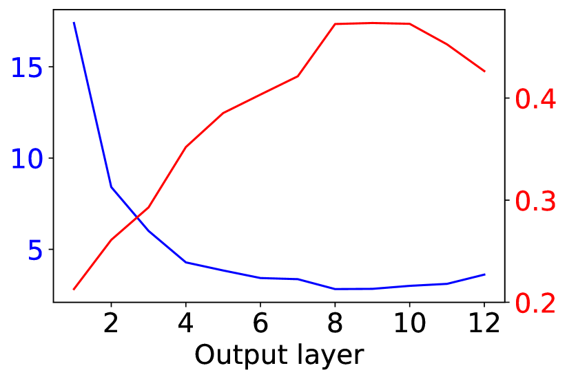
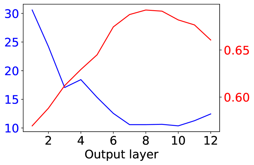
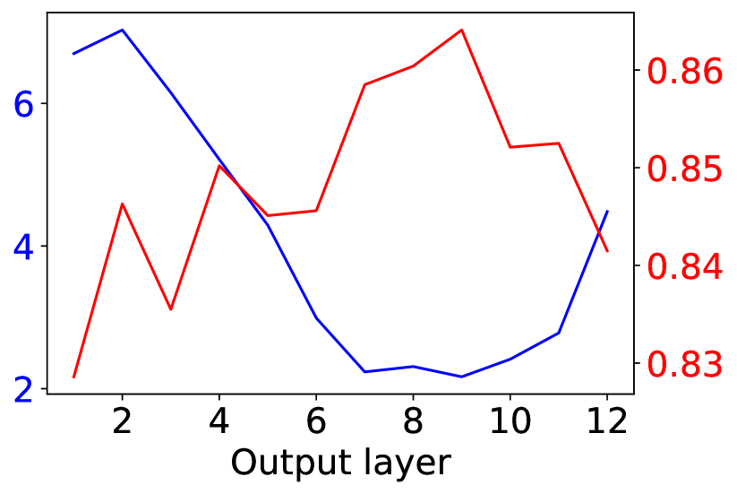
We computed the task-specialty metric for all the 12 layers and plotted with each layer’s probing performance in Figure 9 as we did in Figure 3. For all the tasks except SST-2, we can observe the same pattern as in RoBERTa: the layers with low tend to have high probing performance. On SST-2, the task-specialty metric isn’t negatively correlated with the probing performance. This might be an example mentioned in Limitations that the layers with high can also achieve good performance.
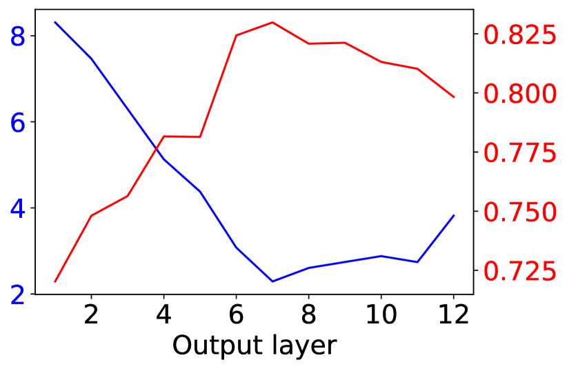
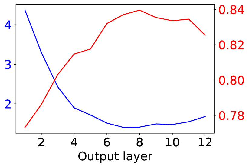
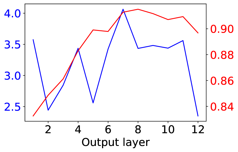
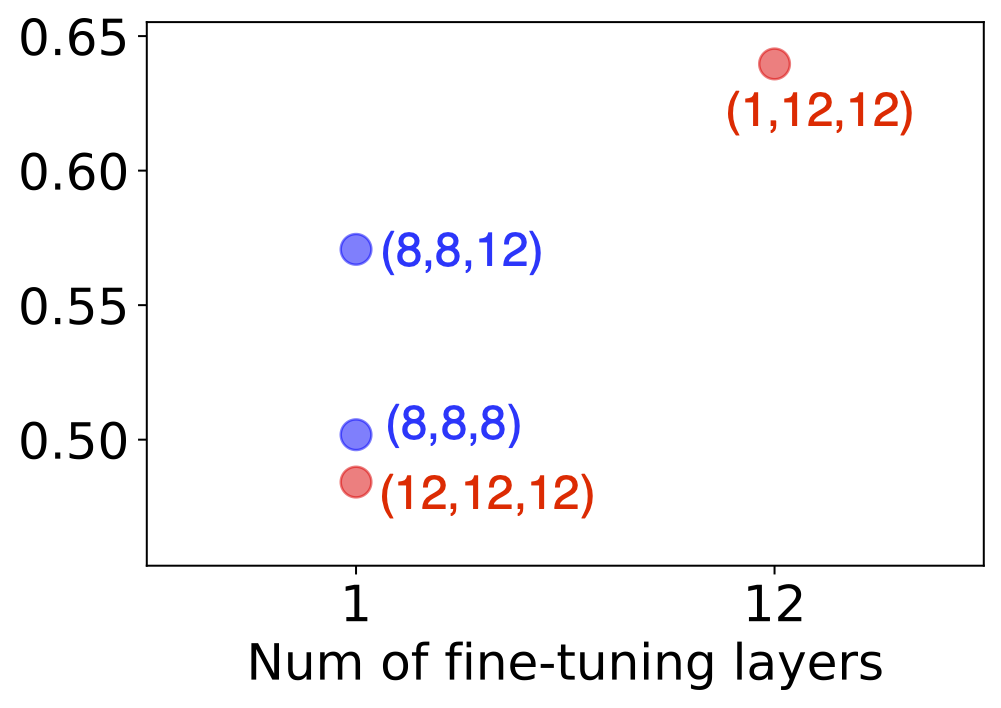
Because the best layer selected by the metric is already the last layer for SST-2, we implemented our strategies , on all the tasks except SST-2. We compared them with baseline and full fine-tuning to see whether the metric can help make fine-tuning more efficiently. The results are plotted in Figure 10 and listed in Table 11. When only fine-tuning layer, our strategy always achieves the best performance and the baseline is always the worst. On MRPC, QNLI and QQP, the performance of is even close to the performance of full fine-tuning with fewer than 10% tuning parameters.
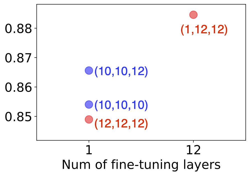
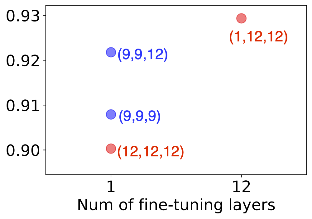
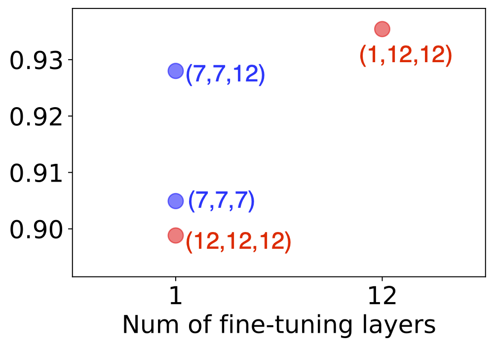
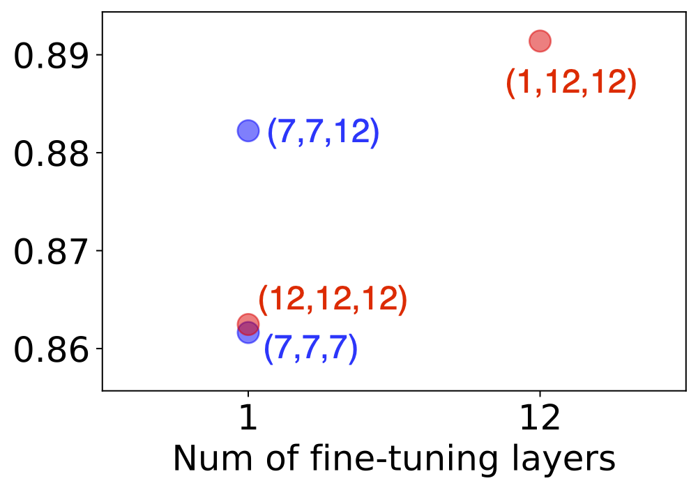
| Strategy # tuned layers | CoLA () | MNLI () | MRPC () | QNLI () | QQP () | |||||
|---|---|---|---|---|---|---|---|---|---|---|
| mean | std | mean | std | mean | std | mean | std | mean | std | |
| 0.502 | 0.0137 | 0.854 | 0.0008 | 0.908 | 0.0083 | 0.905 | 0.0023 | 0.862 | 0.0004 | |
| 0.571 | 0.0111 | 0.866 | 0.0027 | 0.922 | 0.0065 | 0.928 | 0.0011 | 0.882 | 0.0014 | |
| 0.484 | 0.0122 | 0.849 | 0.0008 | 0.900 | 0.0057 | 0.899 | 0.0019 | 0.862 | 0.0015 | |
| 0.640 | 0.0096 | 0.885 | 0.0013 | 0.929 | 0.0038 | 0.935 | 0.0023 | 0.891 | 0.0007 | |
We also compared with middle layer baseline on MNLI. The results are listed in Table 12. works better than this time.
| Strategy # of tuned layers | MNLI | |
|---|---|---|
| mean | std | |
| 0.854 | 0.0008 | |
| 0.866 | 0.0027 | |
| 0.849 | 0.0009 | |
| 0.872 | 0.0022 | |
C.3 Task-Specialty vs. Probing Performance for Pretrained Models
As discussed in section 4.1, we regressed the probing performance on . The regression results are in Figure 11.
C.4 Task-Specialty vs. Probing Performance After Full Fine-Tuning
As discussed in section 4.1, we fully fine-tuned a RoBERTa on each task and obtained the and probing performance of the fine-tuned models. The results are presented in Figures 12 and 13.
C.5 About Computing Task-Specialty Using the CLS Token States
As discussed in section 4.4, we computed using the CLS token hidden states and found that the curves would become less trustable. The curves are in Figure 14.
C.6 Robustness to Data Imbalance and Data Scarcity
As discussed in section 4.4, we conducted a series of experiments with SST-2 and MNLI to verify how sensitive our metric is to data imbalance and data scarcity. For each experiment on SST-2, we had to decide on two key quantities: the number of training examples and the portion that are drawn from the negative group. In other words, we built a dataset by sampling examples from the negative group and examples from the positive group. For the data-imbalanced experiments, we fixed and used . For the data-scarce experiments, we fixed and used .
For MNLI, we need to decide the sample size of each class because it is a classification task with three classes. We use to denote the sample size of the three classes. For the data-imbalanced experiments, is chosen from . The total number is always to avoid the effect of data amount. Similarly as in section 4.4, we plotted and and in Figure 15. Our metric is robust to data imbalance on MNLI.
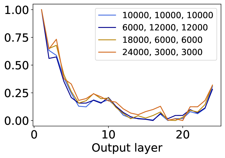
For the data-scarce experiments, is chosen from . The sampled dataset is always balanced. We plotted and and in Figure 16. Our metric has the same trend on MNLI with more than a few thousand samples. This conclusion is consistent with the conclusion on SST-2.
C.7 About Alternatives to Our Task-Specialty Metric
Canonical correlation analysis.
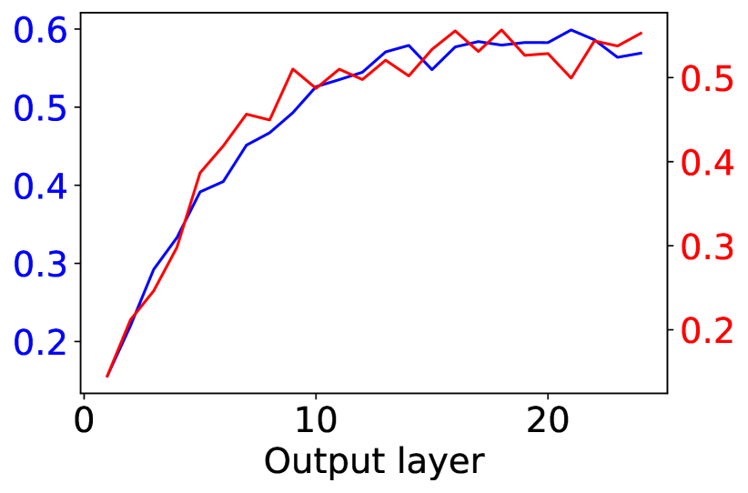
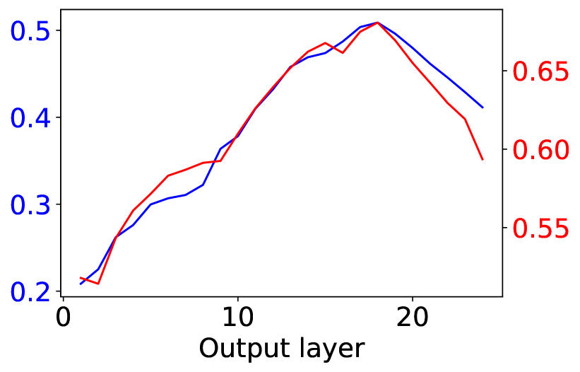
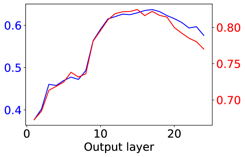
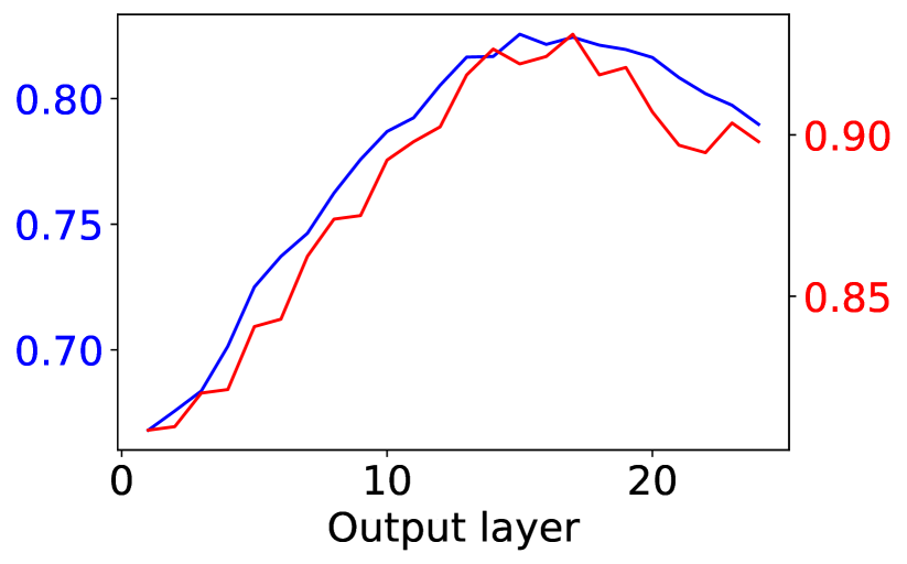
As discussed in section 4.3, a potential alternative to our proposed metric is the canonical correlation between the hidden states and the class labels . Hidden state vectors and one-hot vectors can be viewed as i.i.d. samples from random vectors and respectively, whose relationship can be quantified by canonical correlation analysis. It maximizes the correlations between linear projections of paired samples from these random vectors (or “views"): . The subsequent directions , maximize the same correlation subject to each new projection being uncorrelated with others in the same view for , where is the dimension of hidden states. The algorithm thus provides correlation values. The CCA score is measured as the average over all but the last correlation. This is based on the assumption that the last direction measures noise correlations. This assumption is confirmed by our empirical observation that the last correlation values are always close to zero (of the order 1e-2).
The CCA score are plotted in blue curves and the probing performance of the pretrained model are plotted in red curves in Figure 17. They almost overlap under different y-axes.
In order to ensure computational stability, the sampled auto-covariance matrices of and are perturbed by small constants, and , along the diagonal (De Bie and De Moor, 2003). For each GLUE task we sample class-balanced data-points from the train set. In order to choose the regularization parameters and to avoid overfitting, we perform 10-fold cross validation by using eight of the ten splits to learn the linear projection matrices for different values of and . We use one of the two remaining splits as development set and the other one as test set. The correlation for the development set is evaluated using the learned projection matrices and the best performing pair is then used to evaluate the test set score. We repeat this procedure thrice for each of the two samples of data points. We experiment with different values of . Some of the previous work, although using CCA for representation learning, follows the same scoring procedure to choose the regularization parameters and the corresponding projection matrices (Wang et al., 2015).
CCA has been previously used to measure similarity of layer-wise representations within and across neural network models (Raghu et al., 2017), and to measure similarity of the layer-wise word-level representations with off-the-shelf embedding maps (Pasad et al., 2021). Williams et al. (2019) use CCA to correlate grammatical gender and lexical semantics by representing the discrete gender class as a one-hot vector.
Numerical Rank.
As discussed in section 4.3, the rank-based metric is where . Each can be viewed as measuring the sparsity of the singular values of because . It is an approximation of , i.e., the rank of matrix .
Mutual information.
Discrete mutual information (MI) gives a measure of mutual dependence between two discrete random variables. We use MI dependence between the sentence representations and the corresponding GLUE task labels as a measure of layer-wise task specificity. In order to discretize continuous-valued sentence representations, we run k-means clustering to obtain discrete clusters, as in Voita et al. (2019a). This measure has been previously used to measure the phone and word content in layer-wise representations of a pre-trained speech model (Pasad et al., 2021).
In our experiments, we sampled class-balanced data-points. We held a tenth of these samples out and ran the k-means clustering algorithm with clusters on the sampled data. Then the categorical ID of each held-out sample is defined to be the ID of the learned cluster that it was assigned to. However, after extensive tuning, we still could not obtain any mutual information numbers that look reasonably high: actually, all the numbers were close to zero and they didn’t differ much. We believe that the difficulty stems from the fact that learning clusters is unsupervised and unsupervised learning is known to be difficult. Indeed, if we just use the class labels as the cluster IDs, we can observe a neat clustering—that is why our proposed metric is effective. However, it seems extremely difficult to learn that clustering in an unsupervised fashion.